
Subseasonal-to-Seasonal Forecasting for Wind Turbine Maintenance Scheduling


1
Department of Electronic and Electrical Engineering, University of Strathclyde, Glasgow G1 1XQ, UK
2
School of Mathematics and Statistics, University of Glasgow, Glasgow G12 8QQ, UK
*
Author to whom correspondence should be addressed.
Wind 2022, 2(2), 260-287; https://doi.org/10.3390/wind2020015
Submission received: 22 March 2022
/
Revised: 29 April 2022
/
Accepted: 6 May 2022
/
Published: 12 May 2022
Abstract
:Certain wind turbine maintenance tasks require specialist equipment, such as a large crane for heavy lift operations. Equipment hire often has a lead time of several weeks but equipment use is restricted by future weather conditions through wind speed safety limits, necessitating an assessment of future weather conditions. This paper sets out a methodology for producing subseasonal-to-seasonal (up to 6 weeks ahead) forecasts that are site- and task-specific. Forecasts are shown to improve on climatology at all sites, with fair skill out to six weeks for both variability and weather window forecasts. For the case of crane hire, a cost-loss model identifies the range of electricity prices where the hiring decision is sensitive to the forecasts. While there is little difference in the hiring decision made by the proposed forecasts and the climatology benchmark at most electricity prices, the repair cost per turbine is reduced at lower electricity prices.
1. Introduction
While the skill of traditional Numerical Weather Prediction (NWP)-based forecasts generally decreases with increasing forecast horizon, there are some applications where decisions must be made at longer horizons and therefore longer-range forecasts may be beneficial. In the case of wind energy, turbine maintenance involves activities such as work in the nacelle or crane use, where safety limits apply to the wind speed, so work may only be carried out at low wind speeds. Maintenance tasks also often require the hire of cranes, contractors and other equipment that must be booked in advance, often with a wait time of several weeks. Knowledge of the likely weather conditions can allow for improved scheduling, by allowing an initial decision to be made further ahead or by giving more information than simply relying on the average conditions for the time of year. For example, knowing if a given week is expected to be more or less windy than average could allow planning of the number of jobs to schedule for that week. Extended spells of unusually low wind, sometimes also coupled with high demand due to cold weather, can make power system management more difficult (and expensive); subseasonal-to-seasonal forecasts can give an indication of these unusual conditions further in advance, allowing preparations and corrective actions to be taken [1].
Subseasonal forecasts are generally defined as 10 days to one month ahead, with seasonal forecasts covering one to seven months ahead [1]. They cover the ‘gap’ between conventional weather models and longer-term seasonal predictions. NWP-based forecasts typically have low accuracy beyond the two-week horizon due to imperfect knowledge of atmospheric conditions, an imperfect physical model and the chaotic nature of the atmosphere. However, atmospheric interactions with other systems such as the ocean, ice and soil moisture produce ‘forcing’ effects, and therefore atmospheric changes, on longer timescales [2], which subseasonal-to-seasonal forecasts aim to capture through atmosphere–ocean–ice–land coupling. While the skill of Subseasonal-to-seasonal (S2S) forecasts is not high enough to produce a calibrated probabilistic forecast for a specific hour or day, there is some skill in forecasts averaged over longer periods (e.g., weekly mean conditions) and determining if conditions are likely to be more or less windy than average for that time of year. While by no means a complete description of future conditions, partial information can still aid decision making and planning on these timescales [3,4].
Research in S2S forecasts for energy applications is a relatively new and growing field; the S2S prediction project has been working to ‘improve forecast skill and understanding on the subseasonal-to-seasonal scale’ since 2013 [5] and the S2S4E (Subseasonal-to-Seasonal Forecasting for Energy) project [6] has produced a body of work specific to energy applications in the last 4 years. One of the project’s main outputs was a decision support tool tailored to wind, solar, hydropower and demand forecasts and displaying forecast skill on a coarse grid across the globe. While this will hopefully encourage potential users in the energy industry to consider the benefits of S2S forecasts, the economic value and range of applications and therefore the potential of S2S forecasts in the energy industry has not been fully investigated [7]. The same work also notes some of the key challenges for S2S forecasting, such as: the terminology gap between forecasters and decision makers; the best use of probabilistic information in decision making; the long-term benefits delivered by S2S forecasts versus the immediate benefits demanded by business; and current meteorological modelling limits.
Since meteorological organisations produce forecasts on seasonal timescales from sophisticated models put together by experts, the work on seasonal forecasting for energy focuses on transforming forecasts of weather variables into more relevant energy-system-specific quantities, applying various postprocessing correction methods and evaluating the skill of these forecasts for specific energy applications. A common approach involves implementing Principal Component Analysis (PCA) on the forecasts from all grid points over a large geographical region (for example, the North Atlantic and Europe). This identifies key regimes, or patterns, that can then be linked to variables of interest at the chosen location. This may simply involve finding the variable’s distribution conditional on one of the principal components [8], or making some kind of ‘weather index’, be that an index representing the current phase or amplitude of a certain atmospheric mode such as the North Atlantic Oscillation (NAO) or Madden–Julian Oscillation (MJO) [9], or a value calculated for local conditions from the principal components [10].
Lledò et al. [8] show that forecasts of the MJO can lead to skilful probabilistic daily mean wind speed forecasts up to 36 days ahead. However, they find that the current European Centre for Medium-range Weather Forecasts (ECMWF) forecasts do not reproduce the teleconnections from the MJO phases to European weather and that, currently, strong MJO events are not skilfully predicted more than 10 days ahead. Although the North Atlantic Oscillation accounts for approximately a third of European circulation variability, Lledò et al. [9] examined a wider range of teleconnection indices and found forecast skill from all four tested (the NAO, East Atlantic (EA), East Atlantic Western Russia (EAWR) and Scandinavian Pattern (SCA)). They also note that combining forecasts from different providers improves ensemble mean correlation, and that results can be sensitive to hindcast period length and number of ensemble members. While seasonal forecasting linked to wind speeds often focuses on the most windy winter months [11], Lledò et al. [8,9] examine skill for all seasons separately.
Alonzo et al. [10] used polynomial regression on PCA components to produce a site-specific index with which to produce conditional forecast distributions. Recalibration of the forecast ensembles improved the results and led to calibrated forecasts that were 30% sharper than climatology for their French case study. Cortesi et al. [12] used clustering to identify regimes and map locations and times of year where each regime had particularly strong skill in reproducing wind speeds. Wind energy production has also been forecast on a subseasonal-to-seasonal timescale using capacity factors for three main turbine classes [2]. While this technique allows forecasts to be made for any location without on-site data, this may result in lower skill compared to site-tailored forecasts.
Work has also been done on larger geographical scales, which is needed for electricity system planning or studying whole-country renewable penetration. National demand, wind and solar forecasts were produced for 28 European countries [13], with consistent skill at the 5–11 day horizon but variable skill for longer horizons, depending on the location and specific distribution of renewables. On national aggregation levels, the complex interactions between the electricity system and the weather require a considered approach: Bloomfield et al. [11] used ‘targeted circulation types’ to identify weather drivers for the electricity system in Europe. They note that the strength of response between a weather pattern and the electricity system is strongly dependent on the capacity and location of renewable generation installed. Van der Wiel et al. [14] also defined regimes by their impact on energy variables, rather than the traditional approach that maximises circulation variance explained. They reconstructed 2000 years of data over Europe to examine the skill of S2S forecasts at identifying extreme energy shortfall events (where there is high demand but low renewable generation).
Existing research on maintenance scheduling focuses heavily on decisions specific to offshore wind farms, such as vessel choice [15,16,17,18] or route planning between turbines [16,17,19]. Optimisation of the installation phase, which involves the hire of specialist equipment [20], optimisation of downtime relative to whole power system concerns such as reserves [21] and the prioritisation of maintenance by component type [22] have also been studied. However, perhaps due to the relatively lower cost of maintenance for onshore farms compared to offshore, there has been much less of a focus on maintenance planning for onshore operations. Methods based on maximising the usage of weather windows that have been applied offshore also apply to onshore operations where wind speed safety limits apply, such as crane usage or work in the turbine nacelle.
Barlow et al. [23] note a distinction between the ‘performance’ and ‘condition’ of an asset—for example, an old component that is still operating well may not have resulted in any loss of generation efficiency but its risk of failure has increased. They propose an approach that takes both performance and condition into consideration when deciding when to repair or replace assets. Pelajo et al. [24] combine wind and electricity price forecasts up to 7 days ahead to make a decision on when to take turbines offline for annual maintenance using a cost benefit approach. Their results show a 30% reduction in costs compared to going offline at a random point in the maintenance season. A cost-loss model has also been used for day-ahead go/no go decisions by Browell et al. [25]. They showed that probabilistic forecasts of access windows, as opposed to deterministic, increased the number of days worked and decreased lost revenue. They also note that other works assume perfect forecasts [17,19].
Aside from strategic decisions in the design stage, none of these works consider decisions that must be made weeks ahead, such as crane or additional crew hire. Thus, there is no overlap between the maintenance scheduling literature and the work done on S2S forecasting for renewables.
2. Materials and Methods
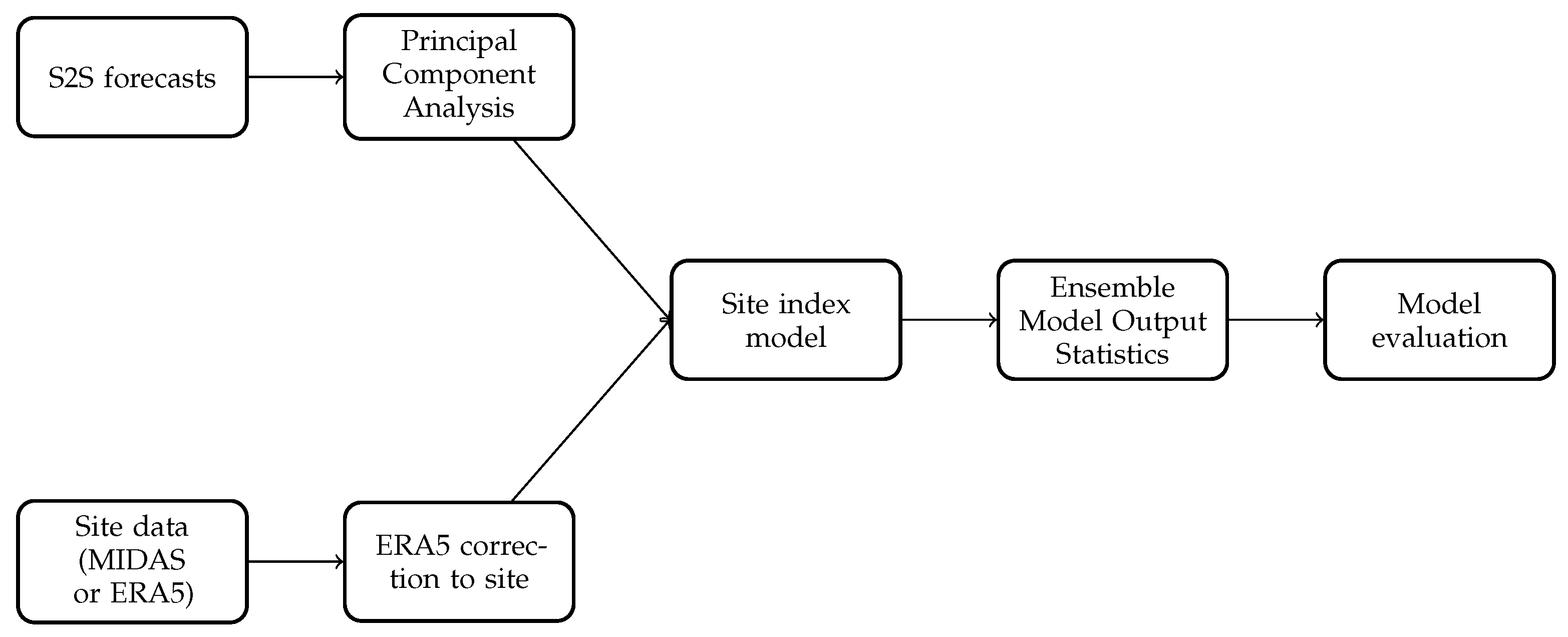
The overall modelling process is laid out in Figure 1 and the individual steps and data partitioning are further explained in the subsequent individual sections. Raw S2S forecasts are available for a grid of locations covering the whole globe and multiple vertical levels in the atmosphere. The methodology presented in this work produces forecasts for task-relevant metrics at the site of interest from these large-scale data with forecasts of specific weather variables.
2.1. Data
ECMWF forecasts of key variables on a grid covering the North Atlantic and Europe region ( N/ W/ S/ E) were downloaded via the S2S database (https://apps.ecmwf.int/datasets/data/s2s, accessed on 11 August 2021) [26]. New forecast runs are produced twice a week and all forecasts available since the 2019 model update were used, from June 2019 to May 2021. Forecast values were downloaded for horizons 0–42 days ahead in 24 h increments. In addition, the same horizons were downloaded for 20 years of hindcasts for each forecast date, i.e., for a forecast on the 1 January 2020, the hindcast dates of 1 January 2019, 2018, etc., were also downloaded. This gave a set of hindcasts over the ‘hindcast times’ 1999–2019 and then a two-year set of forecasts over the ‘forecast times’ June 2019–May 2021. When forecasts were later averaged into weekly values, 1 week ahead included forecasts with horizon 1–7 days ahead, 2 weeks ahead included the 8–14 days ahead forecasts and so on.
Geopotential height and mean sea level pressure are the most common meteorological variables used to study S2S weather patterns as they describe large-scale atmospheric processes on these timescales [8,9,10,12,14]. In addition to this, we included other variables related to hub height wind speed as this is the most relevant height for most turbine maintenance work: any work in, or crane lifts to, the nacelle would use this height for the reference wind speed for safety limits. The average hub height for new onshore turbines is now 90 m [27]. The closest weather model variable to this would be 100 m wind speed, but as the S2S forecasts do not currently have a specific 100 m wind speed variable, several variables related to this (both 1000 and 925 hPa wind speeds and mean sea level pressure) were included as well as 10 m wind speed.
2.2. Site Wind Speed Data
In an ideal world, there would exist measured wind speed data for the site of interest at hub height, possibly at all turbine locations, and for the same time period (1999–2021) as for the ECMWF hindcasts and forecasts. However, very few wind farms have been operating this long and so measured wind farm datasets tend to be much shorter. Therefore, two approaches have been tested: first, we have used wind speed time series from the Met Office Integrated Data Archive System (MIDAS) dataset [28] for weather stations where a complete history over the time period is available. This allows assessment of the skill of the forecasts when trying to model measured wind speeds without extra simulated data. However, the majority of these weather stations measure wind speed at 10 m as opposed to the much taller hub heights of turbines that are of interest. To also quantify the ‘real-life’ skill and usefulness of S2S forecasts, we also used ERA5 reanalysis data from the nearest grid point to selected wind farms and corrected this long time series with the shorter measured time series available from the site itself. A comparison of various reanalysis products for surface and near-surface wind speeds found that the ERA5 data provide the closest agreement with observations [29]. Both of the MIDAS and ERA5 datasets provide mean wind speeds at hourly resolution, allowing for not only the calculation and forecasting of weekly mean wind speed but also of other quantities such as the standard deviation of the hourly wind speed values across the week and metrics relating to specific wind speed thresholds—for example, the proportion of the time that the wind speed is below the safe threshold for work in the hub.
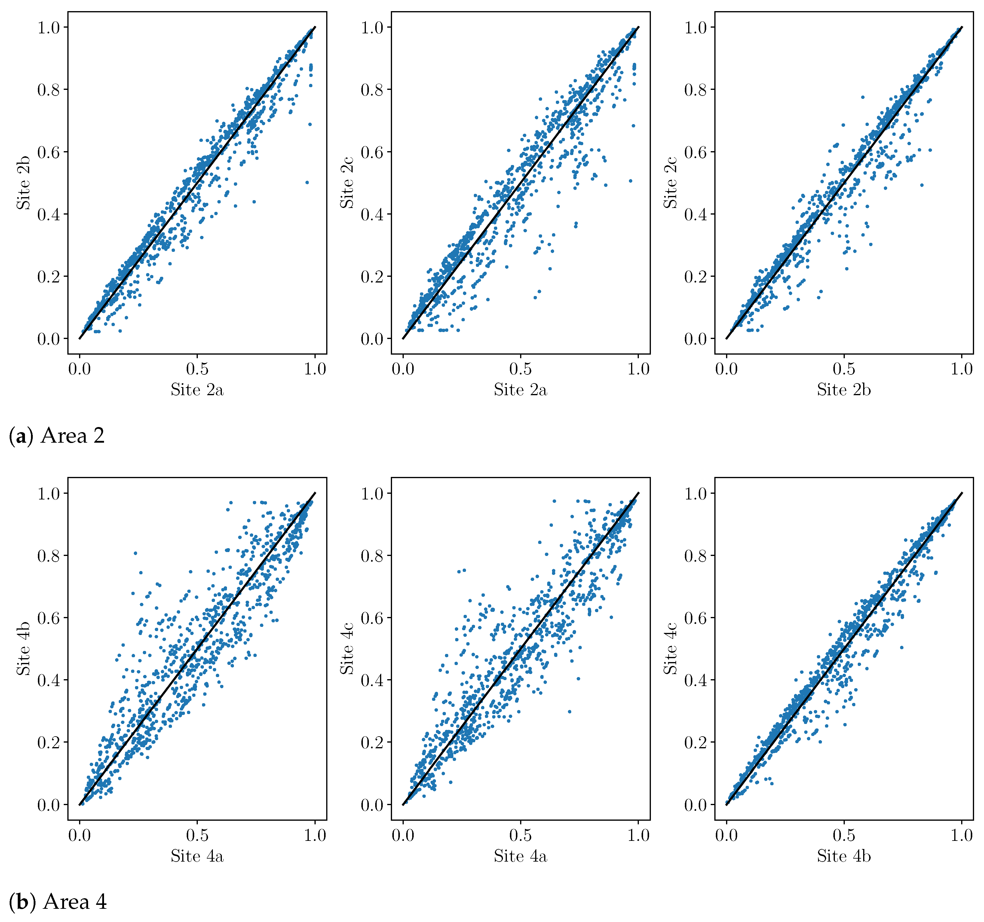
All eight wind farms assessed are in Scotland, with two single farms (WF 1 and 3) and two groups of three geographically close farms (2a, 2b, 2c and 4a, 4b, 4c). The four MIDAS stations selected are those geographically closest to these 4 areas that also recorded wind speed measurements for the required time period and are labelled numerically to match the wind farms (so MIDAS 1 is close to WF 1, etc.).
2.3. Initial Transformations and Corrections
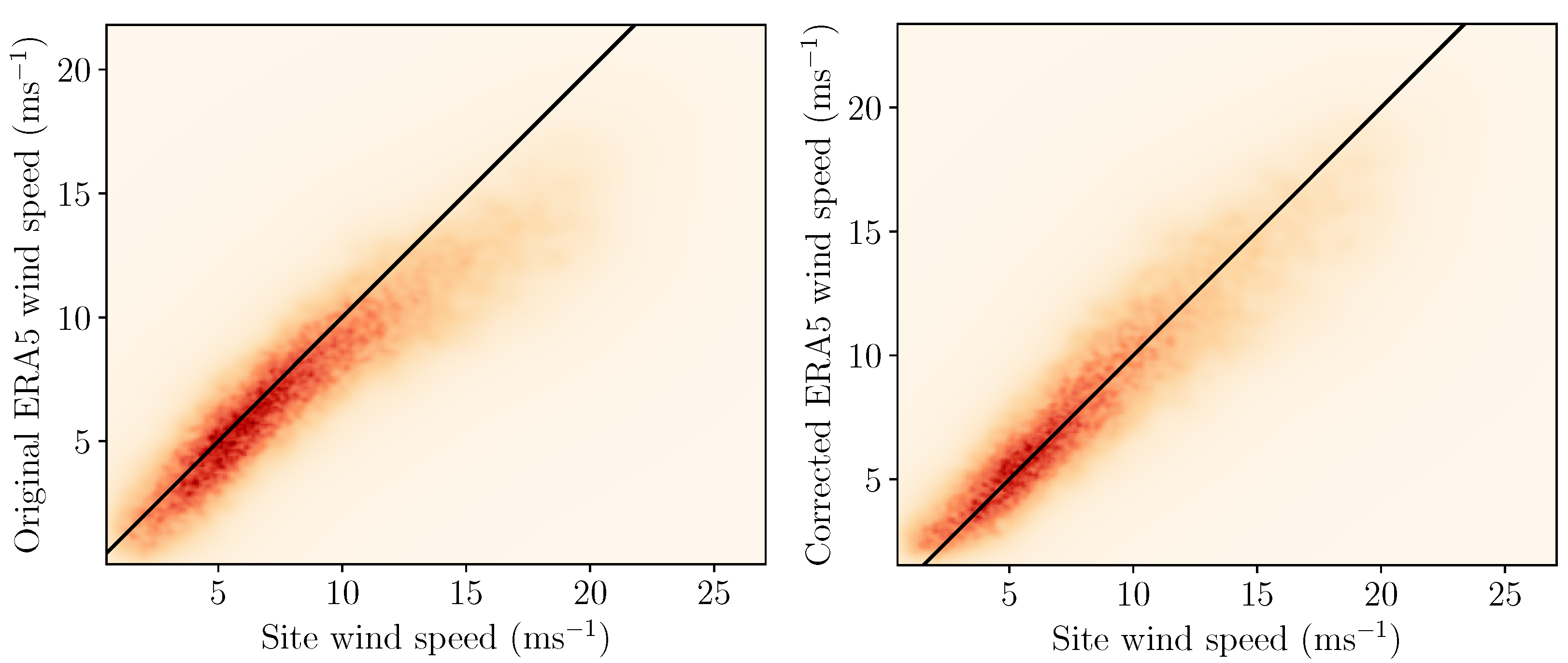
The ERA5 wind speed time series required correction to the site wind speeds through a GAM, with a cubic spline of the ERA5 wind speed along with a cyclical cubic spline () of the day of the year (doy) to account for seasonal variability:
This was implemented with the gam function from the mgcv package in R, using its default numerical optimisation method. The basis dimension of the splines, k, was checked with gam.check to ensure that it was sufficiently large. All available time points were used for training the GAM before predicting the corrected wind speed for all times in the hindcast and forecast sets. This correction is illustrated in Figure 2.
The first step in processing the raw S2S forecasts was to identify the large-scale patterns and atmospheric ‘modes’ present. Principal Component Analysis allows the reduction of multi-dimensional data to fewer dimensions, where the new components are all orthogonal and components account for a sequentially decreasing proportion of variance in the original data. If is a matrix containing all the forecast values for a given variable with each spatial grid point in a separate column (normalised to zero mean) and each time point for a given forecast horizon in a separate row, the transformation matrix to produce the principal components will have dimensions (or if only the first n components are kept) and is made up of the column eigenvectors of the covariance matrix of , such that the eigenvector corresponding to the largest absolute eigenvalue is in the first column and so on. Then, the transformed principal components are given by
The first n columns of give the first n principal components; n was selected so the retained principal components explain 90% or more of the variance in the original data—this is typically 20–40 components for the weather variables used here. Since forecasts are not available for 100 m wind speed directly and several related weather variables are used instead, we have performed PCA on each of these separately, as well as a PCA with them all together, to determine the optimal approach. The zero-hour ahead forecasts for the hindcast times were used to fit the PCA transformation before it was applied to the 1–42 days ahead forecasts for all the available times (both hindcast and forecast times).
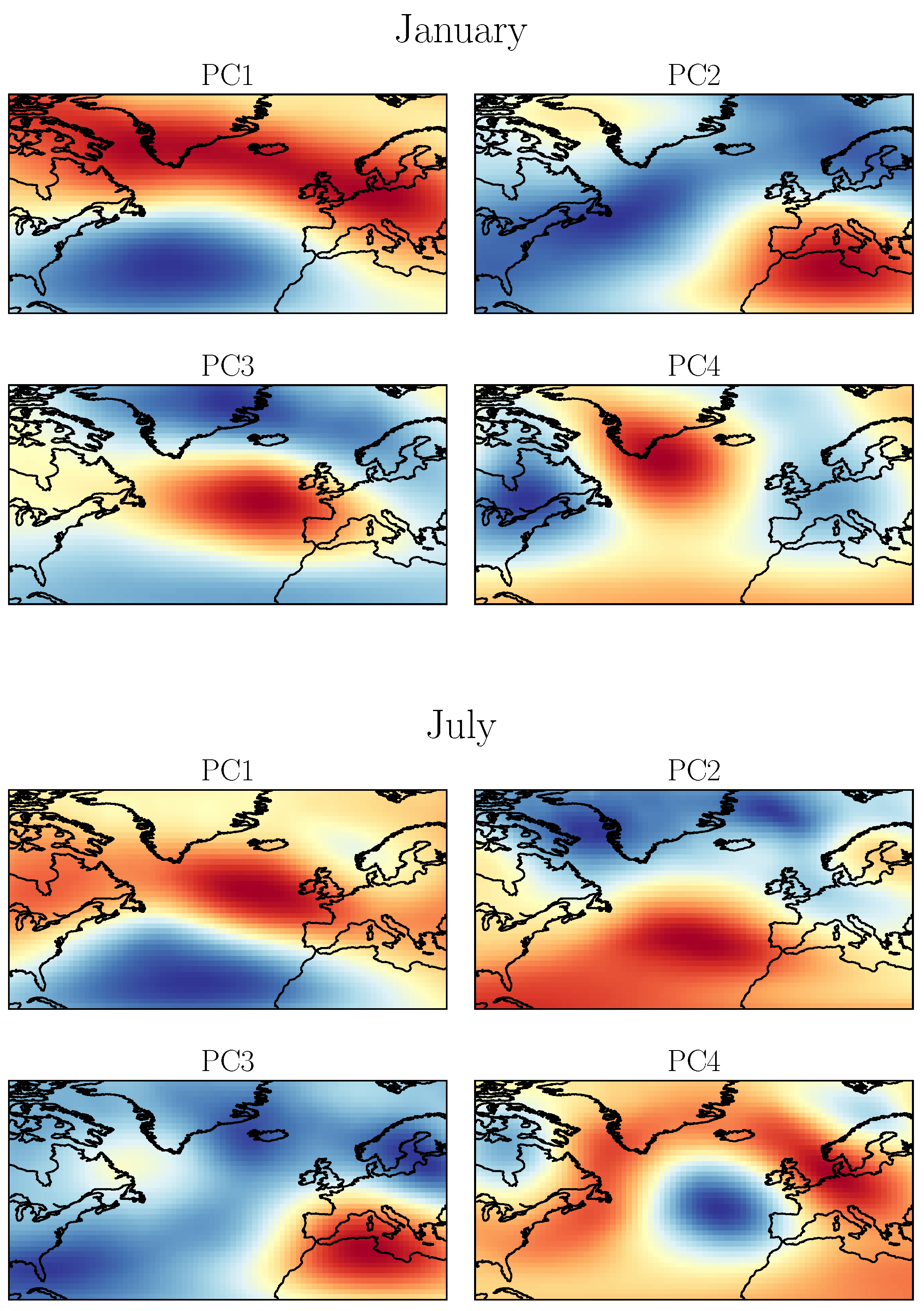
We can also use the ‘reverse’ transformation to project single principal components back onto ‘map’ space, using , with being the ith eigenvector to obtain a map of the ith principal component. This allows us to observe the spatial patterns associated with the principal components, as seen in Figure 3.
2.4. Site-Specific Index Models
While the transformed Principal Component (PC) data now represent the main atmospheric patterns, this is still general to the whole North Atlantic–European region. Therefore, a model is needed to relate the whole-region regimes (represented by the PCs) to the local wind conditions at the site of interest. A similar approach was used by Alonzo et al. [10] with a polynomial regression model to generate site indices. Index models are trained for three different metrics, weekly mean wind speed, weekly standard deviation of wind speed and a ‘useful hours’ index tied to the safety limit for a given task.
Index forecasts for the hindcast time points are required for recalibration of the ensemble index forecasts (the Ensemble Model Output Statistics step), so we must produce out of sample index forecasts for the hindcast times as well as the forecast times. As such, cross-validation is used, where the 20-year hindcast dataset is broken into folds of 2 years each. Index forecasts for each fold of the hindcast times are generated by training on all the remaining hindcast data; however, the year immediately after the test fold is left out of the training folds as there can exist some long-term patterns or correlations in the atmospheric conditions. For example, to generate index forecasts for 2000–2001, all the remaining hindcast times apart from 2002 are used as the training set. To generate index forecasts for the forecast (as opposed to hindcast) times, the entire set of hindcasts is used as the training set. Models are fitted separately for each weekly forecast horizon and forecasts are made for each ensemble member.
2.4.1. Mean Wind Speed Index
Weekly mean wind speed is derived from the hourly wind speeds within the week and is defined as
for the week beginning . The forecast index of weekly mean wind speed is produced by fitting a linear model where the input features are the principal components of the weather variables. If the weekly mean of the ith principal component of the jth weather variable is denoted as ,
A linear model is used to generate indices; as there are many input features (tens of PCs for 3–6 different weather variables), a Least Absolute Shrinkage and Selection Operator (LASSO) approach using regularisation for feature selection is used. This means that instead of finding the optimal coefficients by purely minimising the squared errors, an additional penalty term proportional to the sum of the magnitudes of the coefficients is added to the loss function:
This extra penalty serves to shrink the absolute size of coefficients, which introduces sparsity, and the value of determines the ‘severity’ of this penalty. This is optimised through nested cross-validation on the training set. While, in this model, formulation all the forecast inputs is derived from Principal Components, additional terms such as Fourier terms to model seasonality could also be included. Different configurations of inputs for the index model are tested: extra weekly features (weekly standard deviation, min and max of wind speed) are engineered and included as inputs; and the three weather variables related to 100 m wind speed are transformed into PCs separately to produce three sets of PC, or all together in one transformation. The optimal configuration in terms of whether to group weather variables for the PC transformation, and whether to use extra features, was determined separately for each final index metric using the MIDAS dataset as the ‘real’ wind speeds and is given in Table 1. It is assumed that the relative performance of these different model configurations will be very similar when an index model is trained on the corrected ERA5 data instead of the MIDAS wind speed data, so the same optimal model configurations were used for the remainder of the work.
2.4.2. Variability Index
On the day of a maintenance activity, the measured hub (or crane) height wind speed is the deciding factor as to whether it is safe for a job to go ahead or not. However, when these activities are planned weeks ahead and in whole-week chunks, there is significant uncertainty in the mean wind speed forecast and information about the conditions within the week is lost. Two weeks could have the same mean wind speed while one contains very stable weather for the whole week and one varies between periods of very low and very high wind speeds within the week. Thus, a forecast of the variability of wind conditions within each week is also useful, giving another point of information to base decisions on. This may be particularly relevant when the mean wind speed forecast is close to the safety threshold for the given activity. Standard deviation is used as the measure of inter-week variability and is calculated from the hourly data for that week:
Extra weekly features are derived from the hourly principal components, including weekly standard deviation PC, weekly minimum PC and weekly maximum PC. These are also included in the linear model as linear features with coefficients and , respectively:
Regularisation in the form of a LASSO penalty shrinks coefficients, leading to a more sparse model. The LASSO penalty is applied to all and coefficients in the same way.
2.4.3. Weather Window Indices
The third site index forecast produced links the weather conditions to a specific maintenance task of interest by forecasting the number of hours in the week that are safe to do that task. Each maintenance activity has a safe wind speed limit associated with it and takes a certain amount of time to perform. Therefore, we need a window of at least x hours where the wind speed is always below y ms−1 to perform a given activity. Two obvious metrics to measure this on a weekly basis would be the number of hours in the week below the wind speed threshold, or the number of weather windows in the week. However, there are pitfalls to both of these. Counting the total number of ‘safe’ hours in the week does not tell us anything about the length of weather windows available, so that 10 h below the wind speed threshold could mean a continuous block of 10 h available, or 10 separate blocks of 1 h windows, which is much less useful for a task that takes several hours. If we instead report the number of weather windows of a certain minimum time length, a value of 1 window in a week could mean a single window of the minimum time duration, or that the wind speed is below the threshold for the entire week; the second of these scenarios would allow a lot more work to be done in practice than the first. The final metric used is therefore a combination of these: the number of hours in the week contained in a weather window of a certain minimum length. This way, every hour that is counted is valuable for work as it is guaranteed to be in a usefully long window and there is still a distinction between a single long and a single short weather window. This metric does not differentiate between one long and several shorter windows, but the minimum duration constraint ensures that each window counted is long enough for maintenance activities to be performed in it. Thus, the two parameters defining the weather windows (duration and wind speed threshold) are both determined by the maintenance activity of interest. All weather windows are counted, regardless of whether they fall within the usual working week (9–5 Monday–Friday) or not, as the decision to work at nights or weekends will depend on other factors, including the urgency of the job and availability of staff to work other hours. The number of useful hours metric is the number of hours in the week where wind speed is below p ms−1 for q hours or more at a time and is modelled as
As for the mean wind speed and variability indices, LASSO regularisation is employed for feature selection.
2.5. Ensemble Model Output Statistics
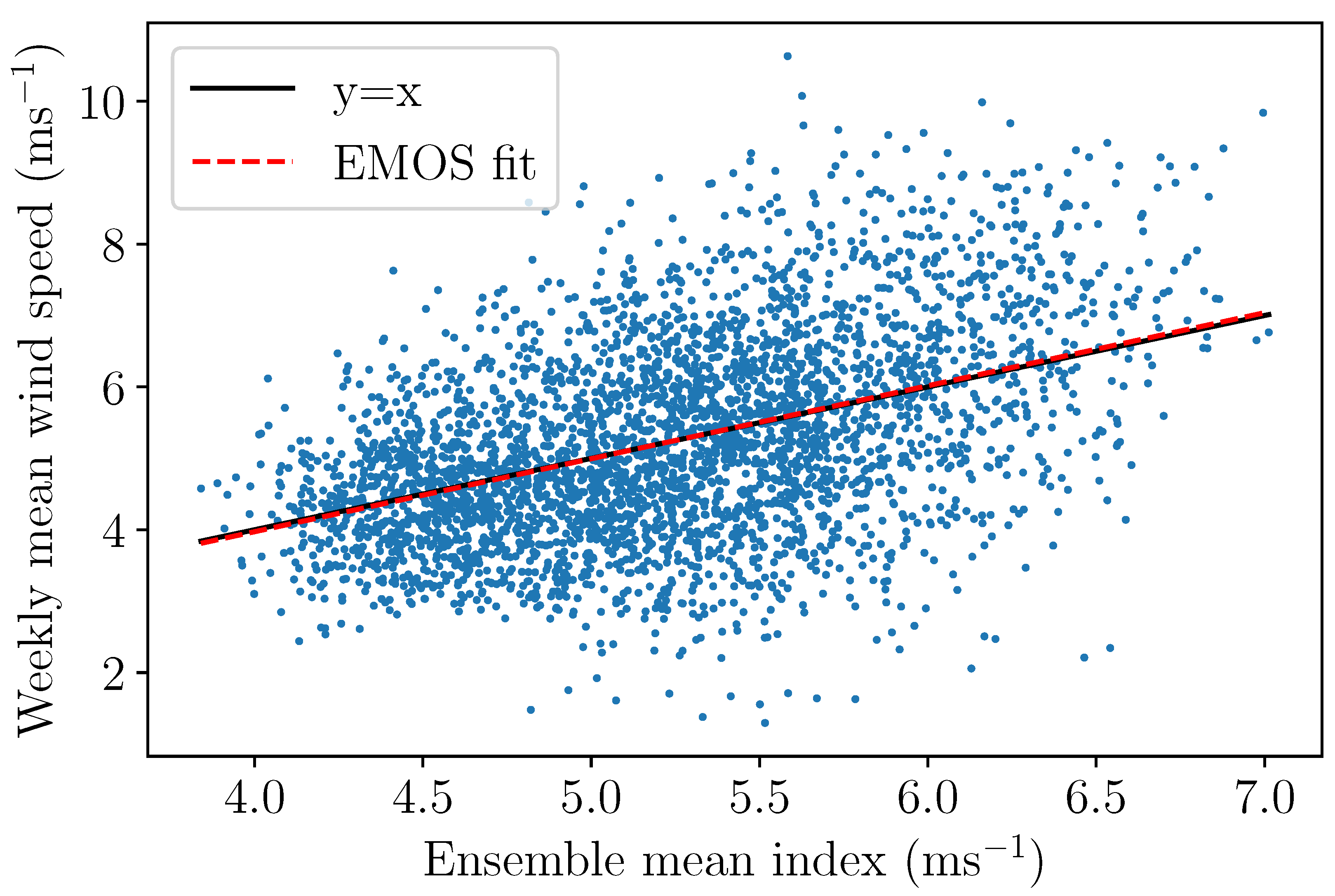
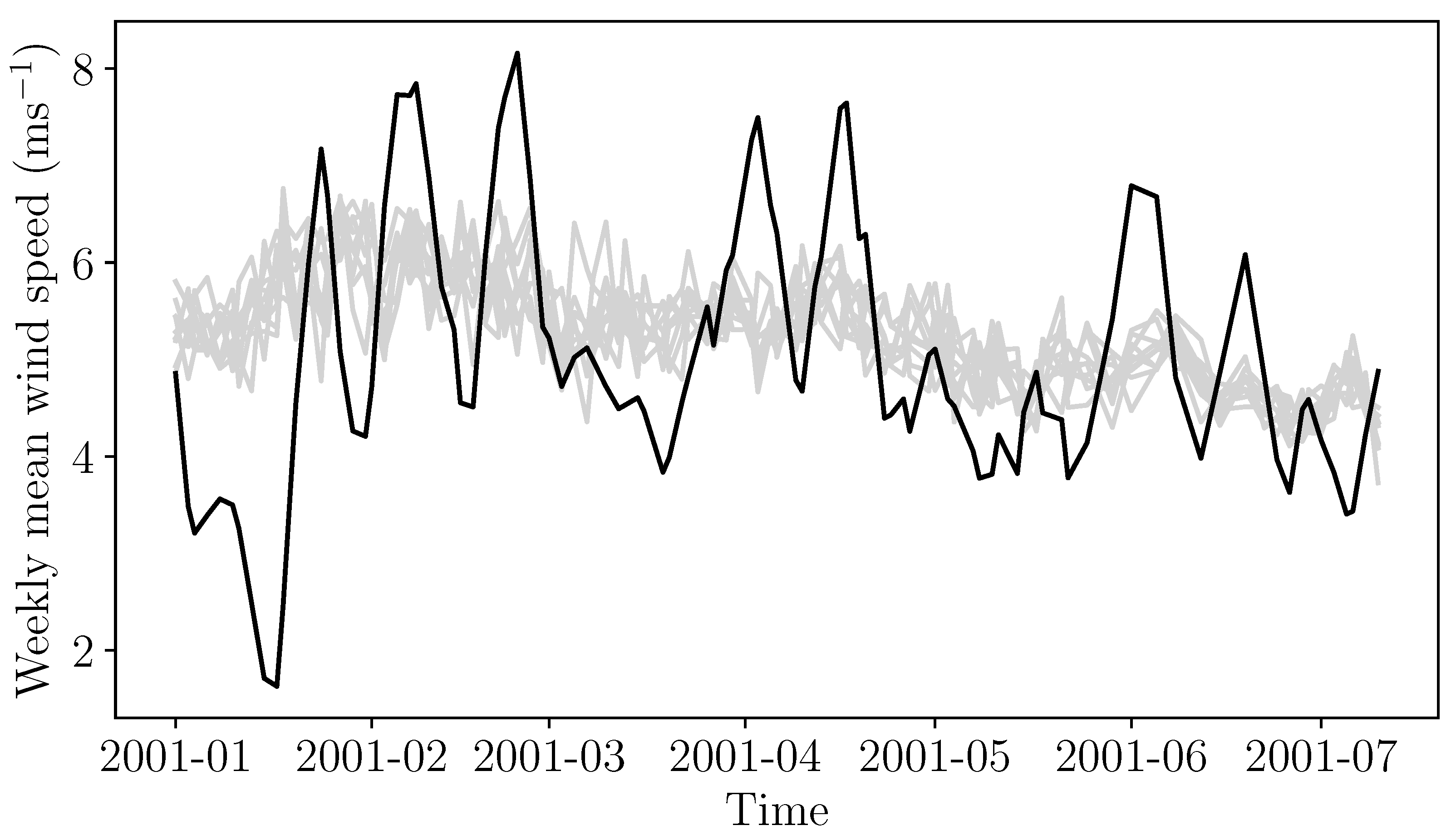
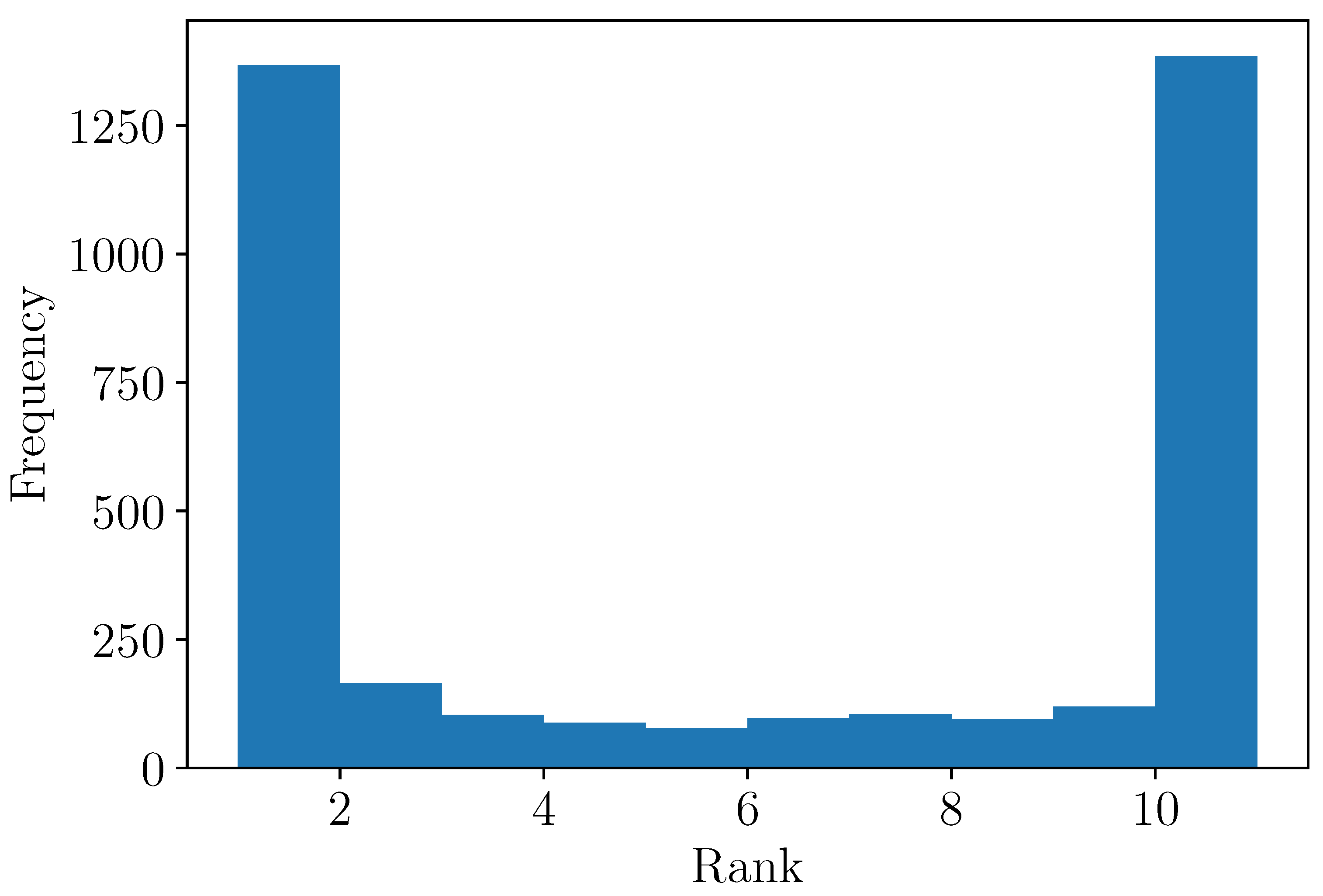
The ECMWF S2S forecasts provide 51 ensemble members, generated through perturbations to the initial conditions for the model run and the model physics. This encapsulates uncertainty information about the forecast as well as simply the ‘best’ single forecast. However, there may still be bias, or over- or under-dispersion of the ensemble members, or both. Ensemble Model Output Statistics (EMOS) aims to correct this to provide a final unbiased, calibrated forecast. From Figure 4, we can see that the index forecasts have virtually no bias, while a time series plot (Figure 5) shows that the ensemble members are significantly under-dispersed—this is also shown by the U-shaped verification rank histogram (Figure 6).
In this work, the EMOS method used is similar to that in Schuhen et al. [30] and is based on the fitting of a parametric distribution to features of the ensemble members in the framework of a Generalised Additive Model of Location, Scale and Shape (GAMLSS) [31]—so all distributional parameters, not just the mean, can be modelled explicitly. The choice of parametric distribution to fit was aided by the R function fitDist from the gamlss package, which allows the fitting of a group of possible distributions with the optimal distribution having the lowest AIC score. In fitDist, all distributions are fit with constant values for all parameters; this is then used to select a distribution that more closely matches the overall distribution of the target variable. For the mean wind speed and variability indices, the set of ‘realplus’ distributions were considered, as wind speeds (and their standard deviations) may only take real positive values. The gamma distribution was found to most closely fit the real distribution of weekly mean wind speeds and variabilities so this was used as the base parametric distribution to fit the EMOS correction model (a GAMLSS). The gamma distribution has two parameters, location and scale . First, we define two metrics of the K ensemble index forecasts , their mean value and mean difference [32]. This value of mean difference takes into account the distance between each pair of ensemble members, and is less sensitive to outliers compared to measures such as standard deviation.
The two gamma distribution parameters and can then be modelled as functions of and
giving the final forecast distribution
The coefficients are estimated by maximum likelihood using the gamlss function and log link functions in Equations (11) and (12) to ensure positive values for and .
A different distribution was needed for the weather window index forecasts, as the number of available hours in a week is bounded at zero and 168. This can be normalised to span [0, 1] and will have probability masses on the bounds, as any week with a consistently high wind speed will have zero available hours and there are also weeks where the whole week is in a weather window. Therefore the zero and one inflated Beta distribution (BEINF) is chosen as the parametric distribution to fit in the EMOS stage for the weather window index forecasts. The BEINF distribution has 4 parameters, which in R are the location , scale and two parameters related to the amount of probability assigned at zero and one, and . These are modelled as functions of the same ensemble mean and ensemble mean difference as in Equations (9) and (10):
If the relations
are used to convert from location and scale parameters used in R to those more commonly used to describe the beta distribution and the boundary probabilities, the final forecast distribution is given by
where and .
2.6. Benchmark Climatology
It is important to benchmark any proposed method to be able to quantify its performance relative to other methods. For seasonal forecasts, the most common benchmark is climatology, where the forecast is an average of historic values for that particular time of year—in this case, the month of the year. We use the time points equivalent to the range of S2S hindcasts (i.e., 1999–2019) to produce the distribution of target values (e.g., weekly mean wind speed) for each month of the year—this is then the forecast climatology for the forecast times matching those for which we produce model forecasts from the S2S forecasts. Climatology forecasts are produced for both the MIDAS data and the corrected ERA5 site data so that S2S forecasts trained on each may be compared to climatology produced with the same data. Anecdotally, industry users who work on-site use their personal experience of past site conditions at different times of the year to inform their work and decisions—this could be described as an informal type of climatology-informed decision.
3. Results
3.1. Mean Wind Speed Forecasts Trained on MIDAS Data
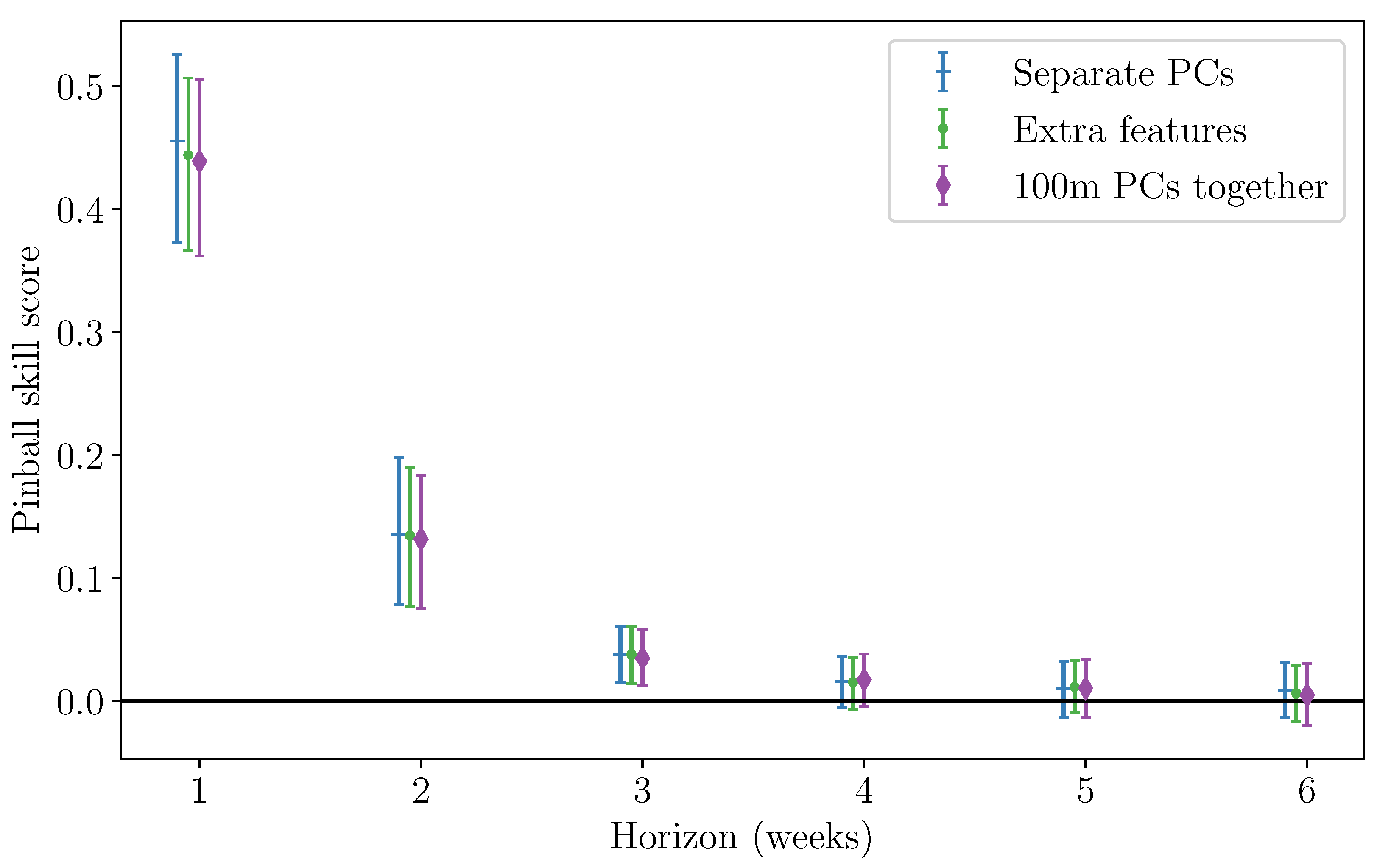
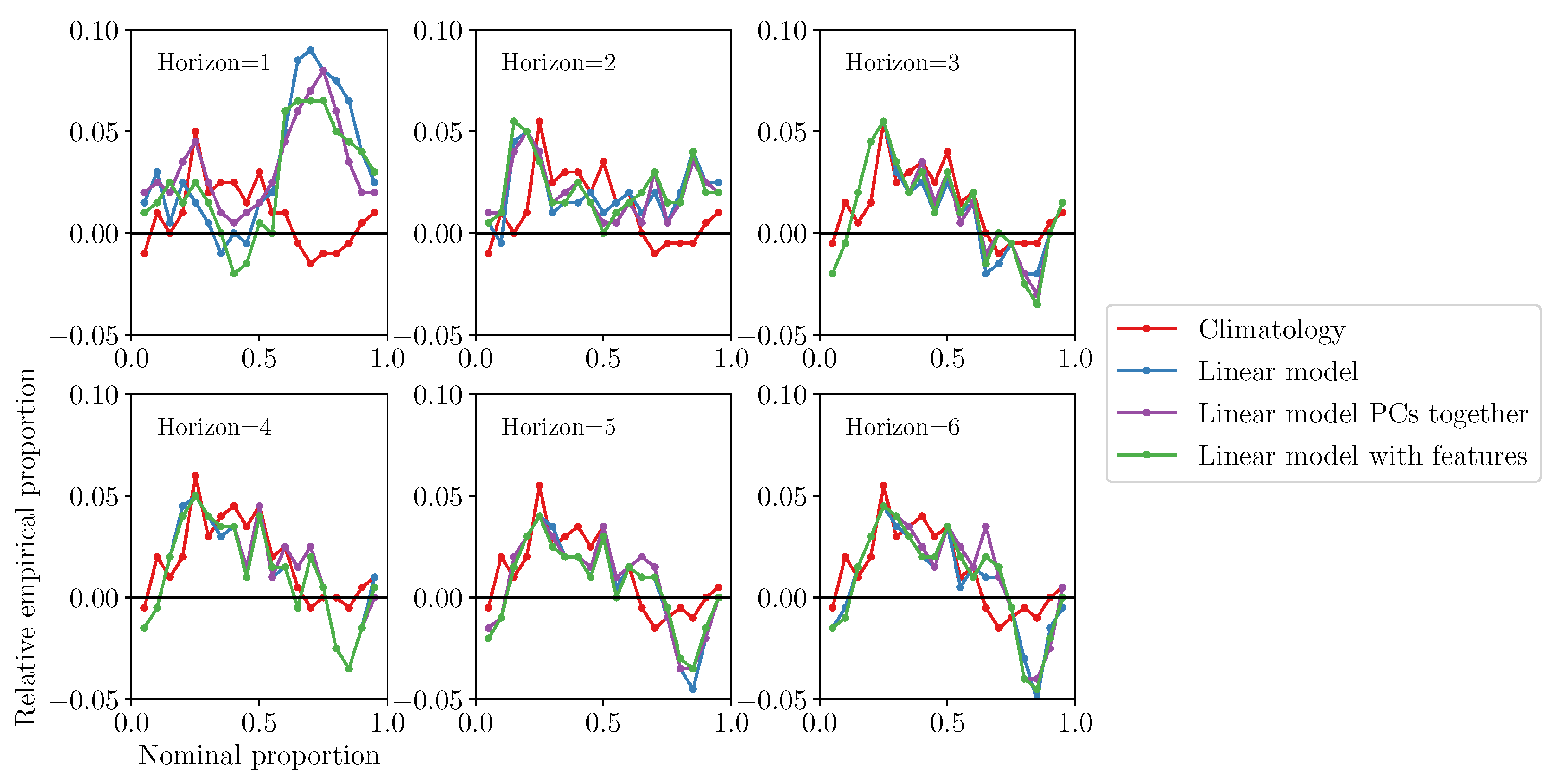
Firstly, two main variations to the model configuration are tested: grouping the weather variables related to 100 m wind speed in one Principal Component transform, and calculating separate sets of PCs for each of these variables. Secondly, we have to choose the features derived from these PCs that are used as inputs to the index model: while PCs and MIDAS data/site measurements are of hourly resolution, index forecasts are produced for weekly intervals. All model configurations take weekly mean values of the PCs as inputs, but it is also possible to provide other features such as weekly standard deviation and minima/maxima for each PC. This may be more relevant when modelling certain metrics such as measures of variability rather than mean values. All these modelling configurations were tested for all the MIDAS sites, with very similar results displayed at all sites and shown for one location in Figure 7. This and all following skill scores are calculated relative to climatology. This shows no significant difference in skill between model configurations, a result which holds across all the MIDAS sites. This initial evaluation of skill also indicates skill above zero up to and including three weeks ahead, which is promising. The metric of Pinball loss used to calculate these skill scores is a function of both the reliability and sharpness of the forecasts. However, a calibrated forecast with a slightly lower skill score is still preferable over a forecast with a better skill score but that is not calibrated. Calibration (or reliability) is displayed in Figure 8. This shows that all variations of the linear model tested display very similar reliability to each other. Since using the 100 m PCs together and not including extra features results in a faster runtime, this model is adopted for the weekly mean wind speed index. However, the extra features are always included for a variability index forecast as the extra features are directly related to inter-week variability, which is the target for this index. The exact features and numbers of principal components used are given in Table 1.
3.2. Mean Wind Speed Forecasts Trained on ERA5 Data
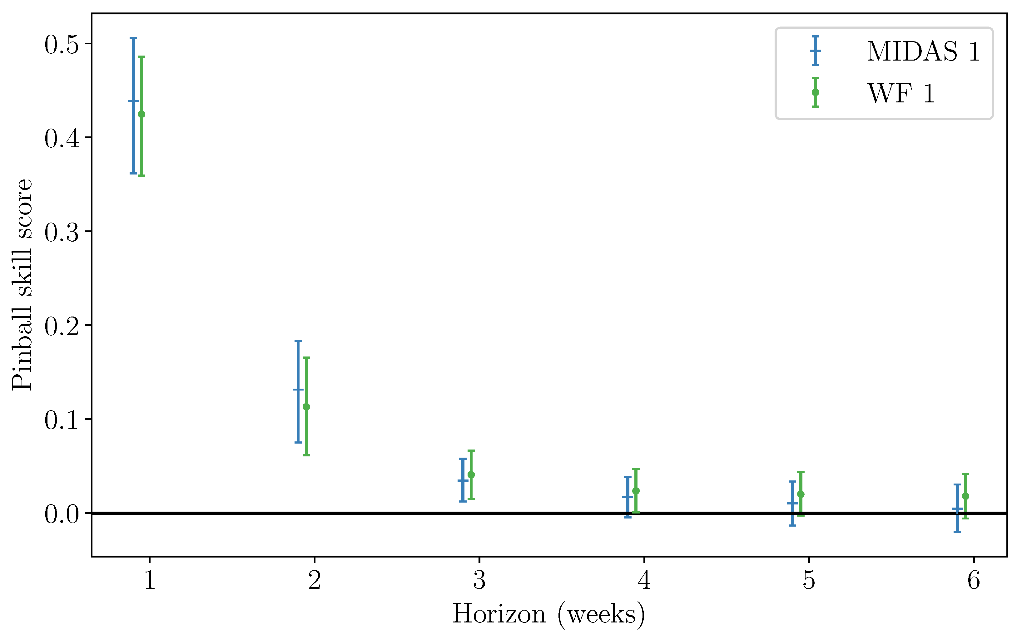
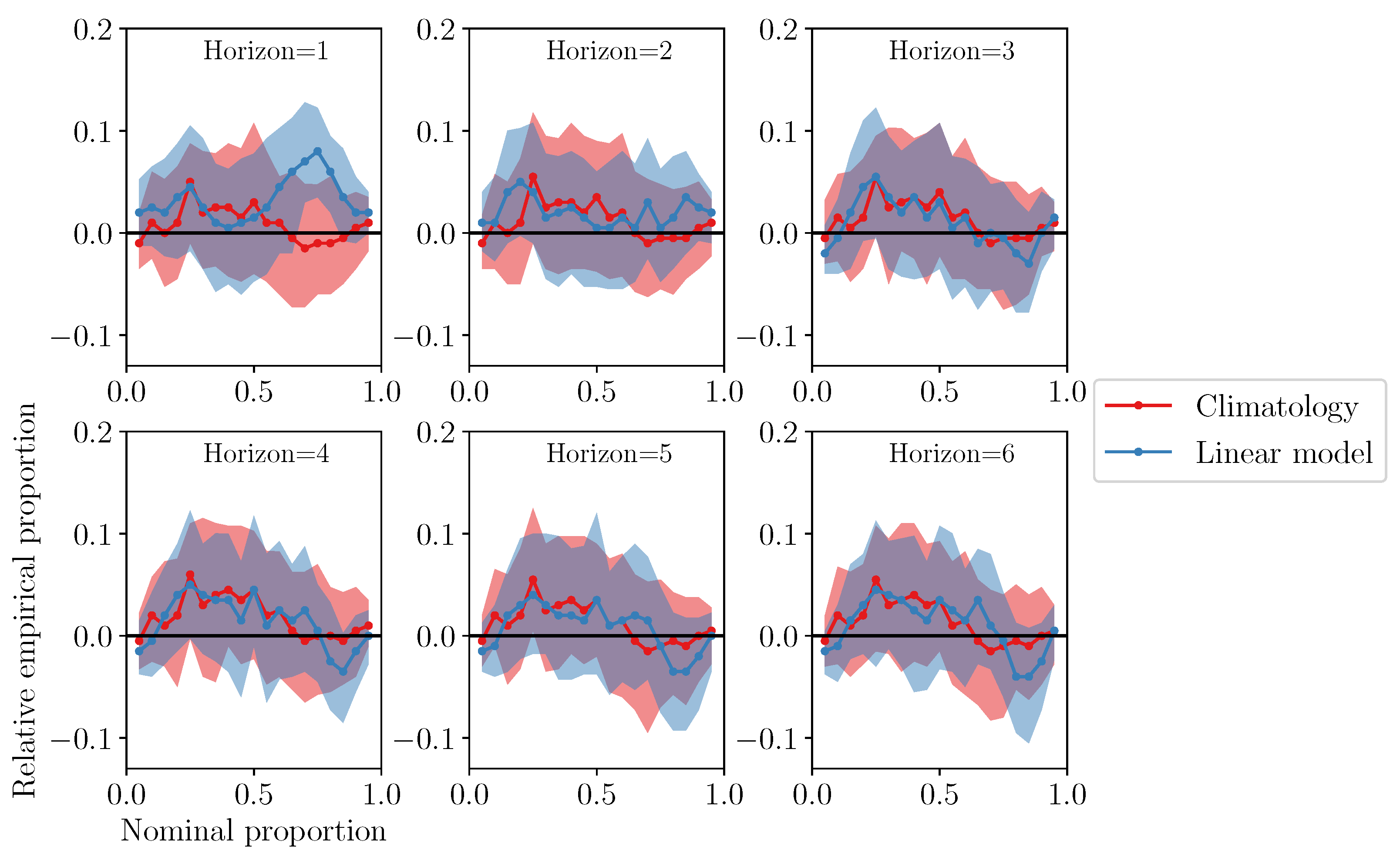
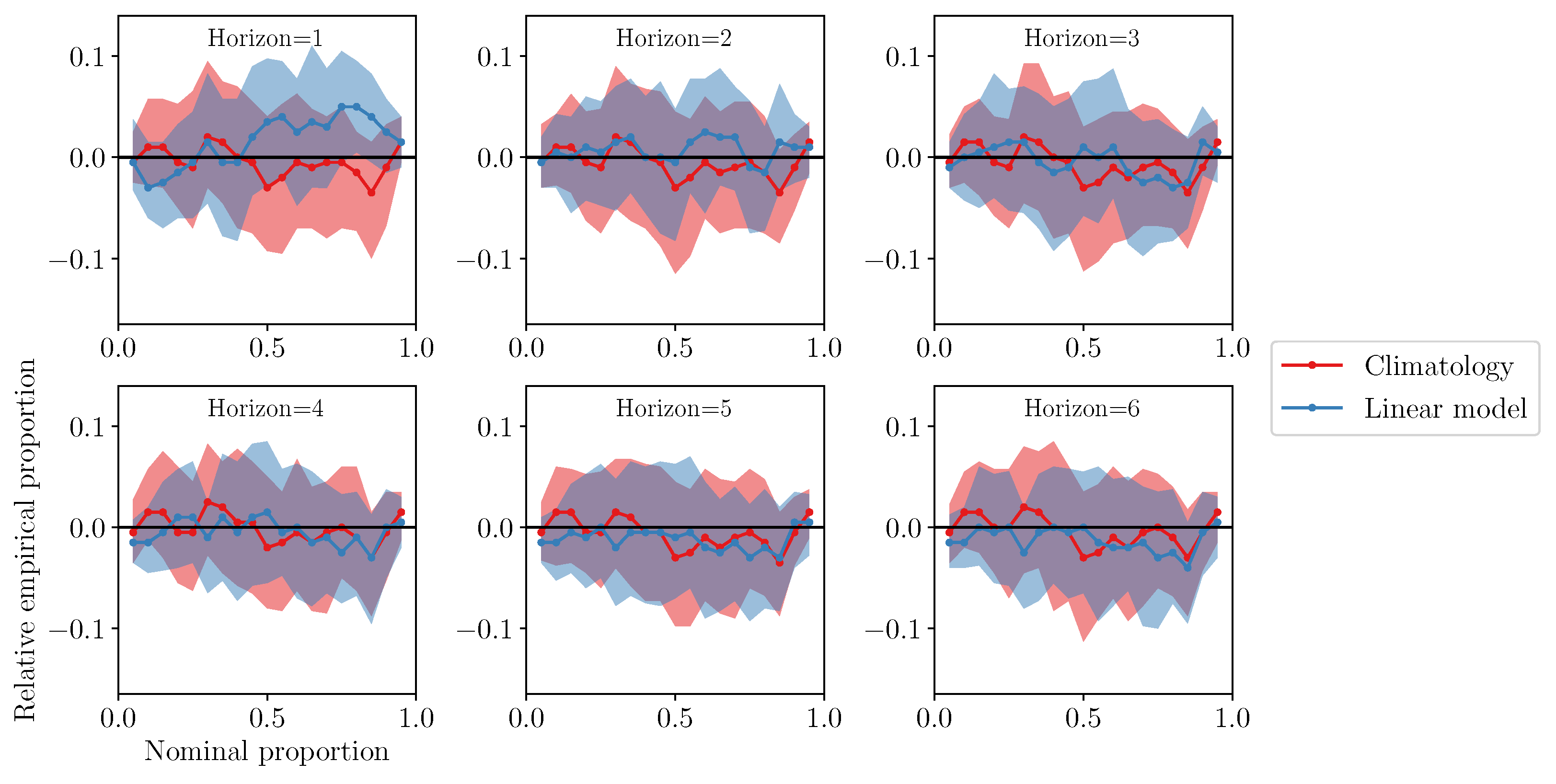
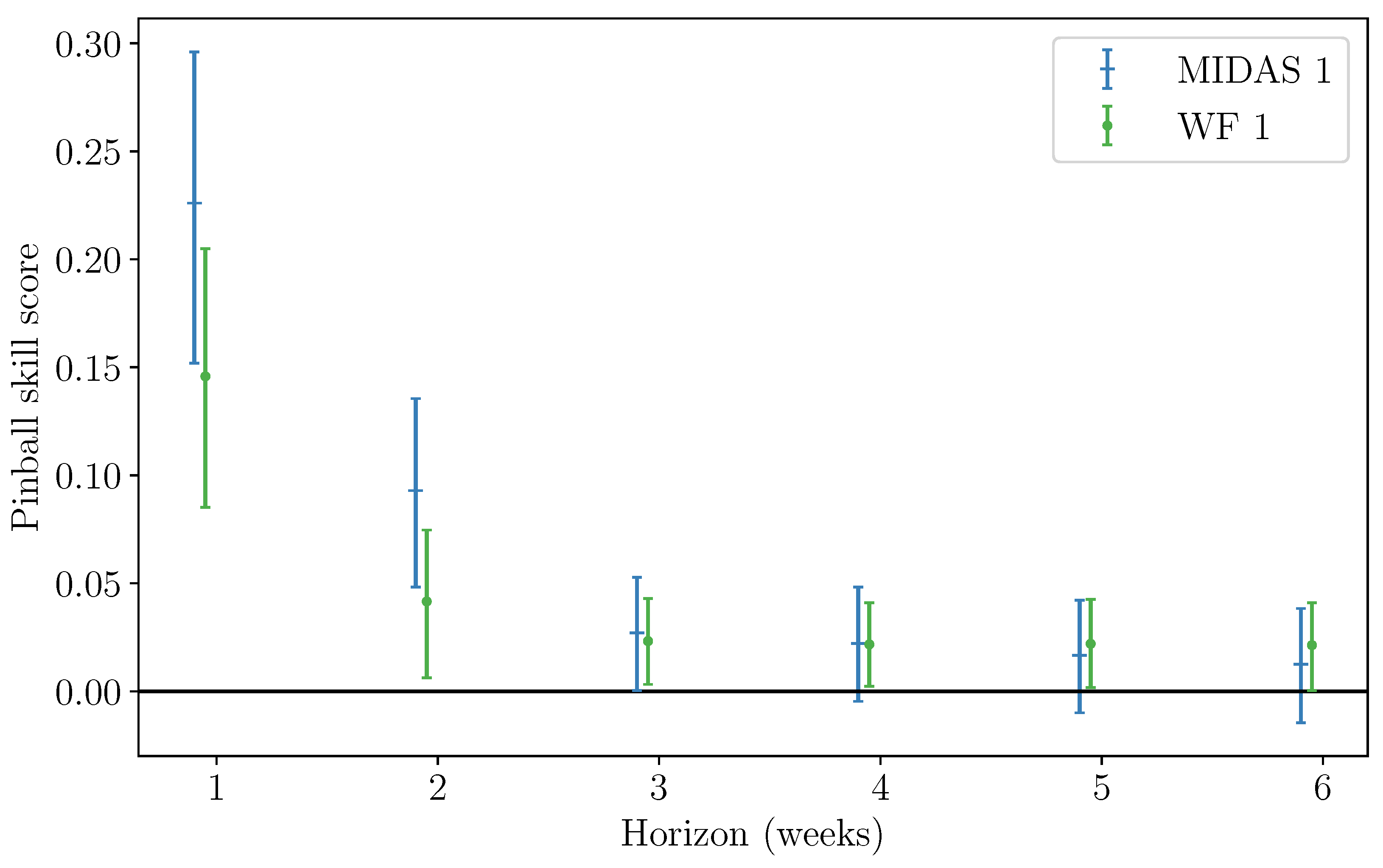
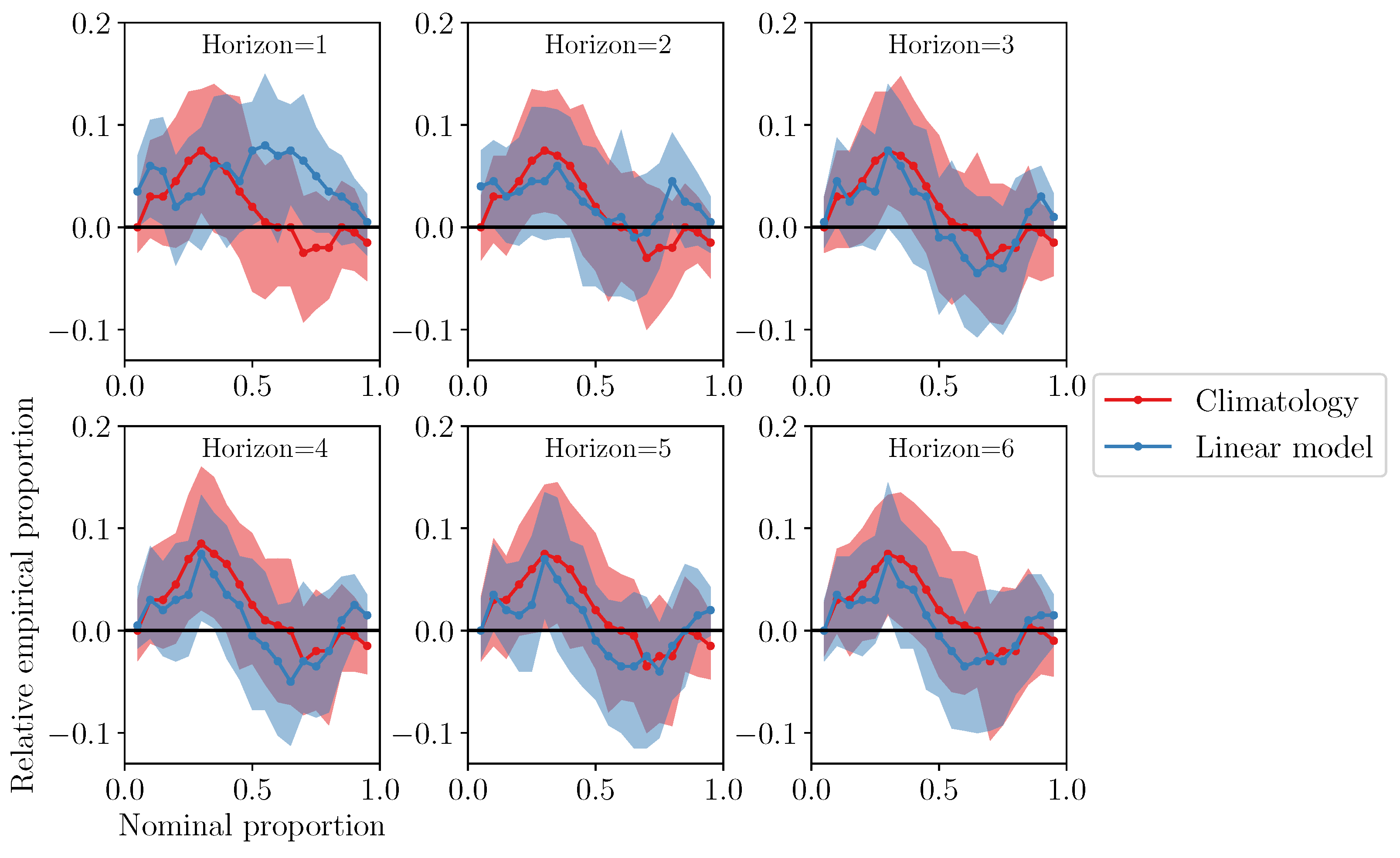
It is assumed that the optimal model configurations for forecasts trained on MIDAS data (grouping 100 m wind-speed-related variables and including inter-week standard deviation as a feature for only the variability forecasts) also hold for forecasts trained on ERA5 data. The skill of the forecasts trained on corrected ERA5 data (for the actual wind farm sites) is presented grouped by location, with area 1 shown in Figure 9 and the remaining three areas in the Supplementary Materials. Forecasts with skill are described as ‘fair’, are ‘good’ and are ‘very good’. This follows the descriptions for skill levels given by the S2S4E project’s decision support tool [3] (s2s4e-dst.bsc.es/#/ (accessed on 11 August 2021)); however, these are purely indicative based on expert judgement, and the skilfulness of a forecast depends on its usefulness in decision making. All the wind farm site forecasts show very good skill one week ahead, fair skill between 0.1 and 0.15 2 weeks ahead and continuing fair skill 3 weeks ahead. The ERA5 forecasts show similar skill to the MIDAS forecasts, with slight increases in skill over the MIDAS forecasts for areas 2 and 4 for the shorter horizons. Reliability diagrams for the MIDAS 1 site and area 1 (based on ERA5 data at WF1) are shown in Figure 10 and Figure 11, respectively. On these plots, a perfectly reliable forecast would lie on the line . Both climatology and linear model forecasts are reliable across the forecast distribution, the only exception being some of the higher quantiles in the one week ahead linear model forecast. This horizon is not the main focus for S2S decision making and, typically, alternative data sources and forecasting methods (based on a standard NWP forecast) would be used for this shorter horizon, so this slight lack of calibration is not hugely important.
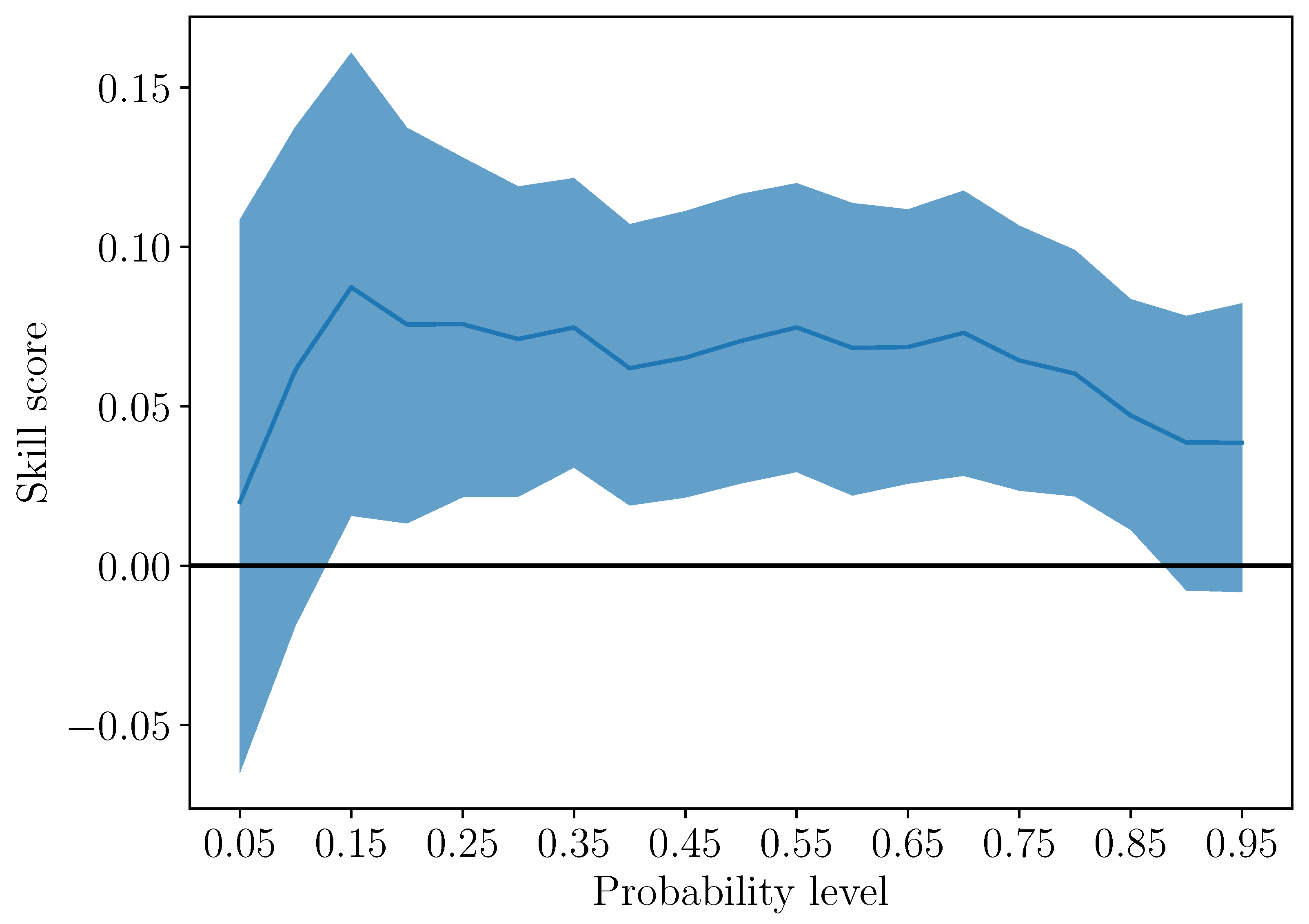
The Pinball skill scores shown in Figure 7 and Figure 9 are an average of the Pinball score across the forecast distribution. However, there may be more skill relative to climatology in different parts of the distribution—for example, the centre vs. the tails. Climatology is calculated for both MIDAS and corrected ERA5 data so each index model is compared to climatology that has been produced from the same data. Figure 12 shows the skill for a 2 week ahead forecast for each quantile level of the distribution. This is still a skill score relative to climatology rather than absolute Pinball values, and shows that there is skill across the whole distribution, with only slightly decreased skill at the most extreme (q5 and q95) quantiles assessed.
For the geographically close groups of sites at areas 2 and 4, it is possible to share resources such as cranes, parts and people easily between sites. As such, it is useful to understand any correlations in forecast performance between these sites. For example, when forecasts are underpredicting at site A, what does this likely mean for forecast performance at site B? To examine this, the realisation value is passed through the inverse cumulative distribution function to obtain the forecast probability of this value occurring. These ‘realisation probabilities’ should be uniformly distributed if the forecasts are calibrated. Because they indicate where in the distribution the real value fell, they can show times of under- or over-forecasting. A scatter plot of these values shows the correlation in the forecast bias between neighbouring sites. Figure 13 shows strong positive correlations between sites, indicating similar simultaneous forecast biases. The least strong correlations (site 4a with 4b and 4c) also correspond to the largest geographical distance between wind farms.
3.3. Variability Indices
The variability index is trained on the standard deviation of measured hourly wind speeds within the week. Figure 14 shows the skill of variability index forecasts for area 1. As for mean wind speed, the MIDAS-based and ERA5-based forecasts give very similar skill, except for area 2 at shorter horizons. In general, the skill of the variability forecasts is lower than that of mean wind speed forecasts for 1–2 weeks ahead forecasts; however, some skill persists to the longer (4–6 weeks ahead) horizons at all sites. Perhaps this is driven by a relationship between large-scale weather patterns and variability—for example, the NAO phase (the sea level pressure difference anomaly between Iceland and the Azores) is related to the number and strength of winter storms in Europe.
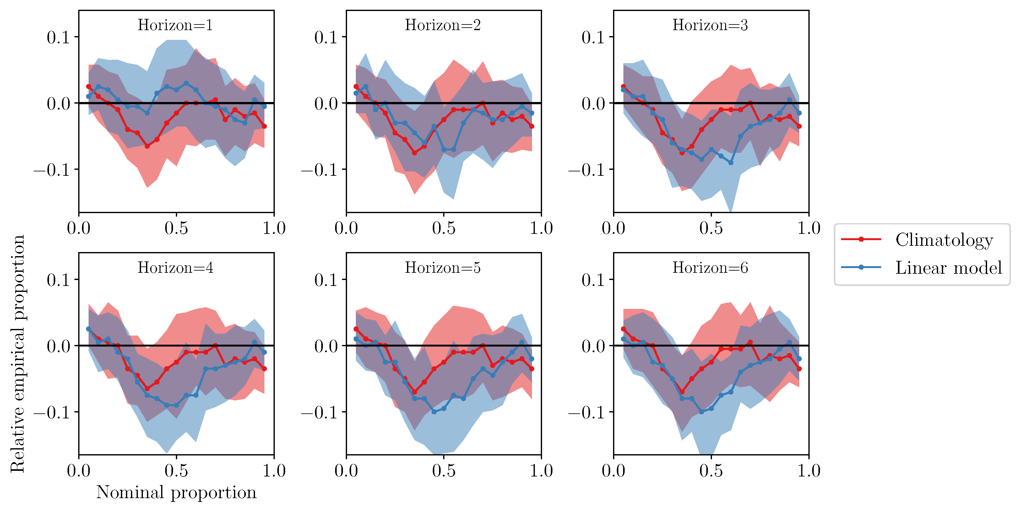
The reliability diagrams for variability forecasts again for both MIDAS (Figure 15) and ERA5 at the wind farm (Figure 16) show generally calibrated forecasts that do not display any consistent forecast bias or over- or under-dispersion. The one week ahead horizon again tends to show the greatest departure from perfect reliability. These observations apply to all locations, with the plots for other areas presented in the Supplementary Materials.
3.4. Weather Window Indices and Economic Value of Forecasts
The weather window indices and subsequent cost-loss analysis are based on an example where a crane is needed for a maintenance task. The safe wind speed threshold for crane use depends on the crane model and object being lifted, but is assumed to be 7 ms−1 in this work (Exact limits are tied to the specific job and equipment and are set out in the ‘authorised work procedure’. Interviews with site operations teams indicated that typical crane lift limits are between 5 and 8 ms). It is also assumed that a minimum of an 8 h window is needed to complete a maintenance task. As an indicative figure, in the 20 years of hindcast data at one site, 50.8% of time points were below the 7 ms−1 threshold. Of the 5003 unique weather windows, 2582 of them lasted 8 h or longer.
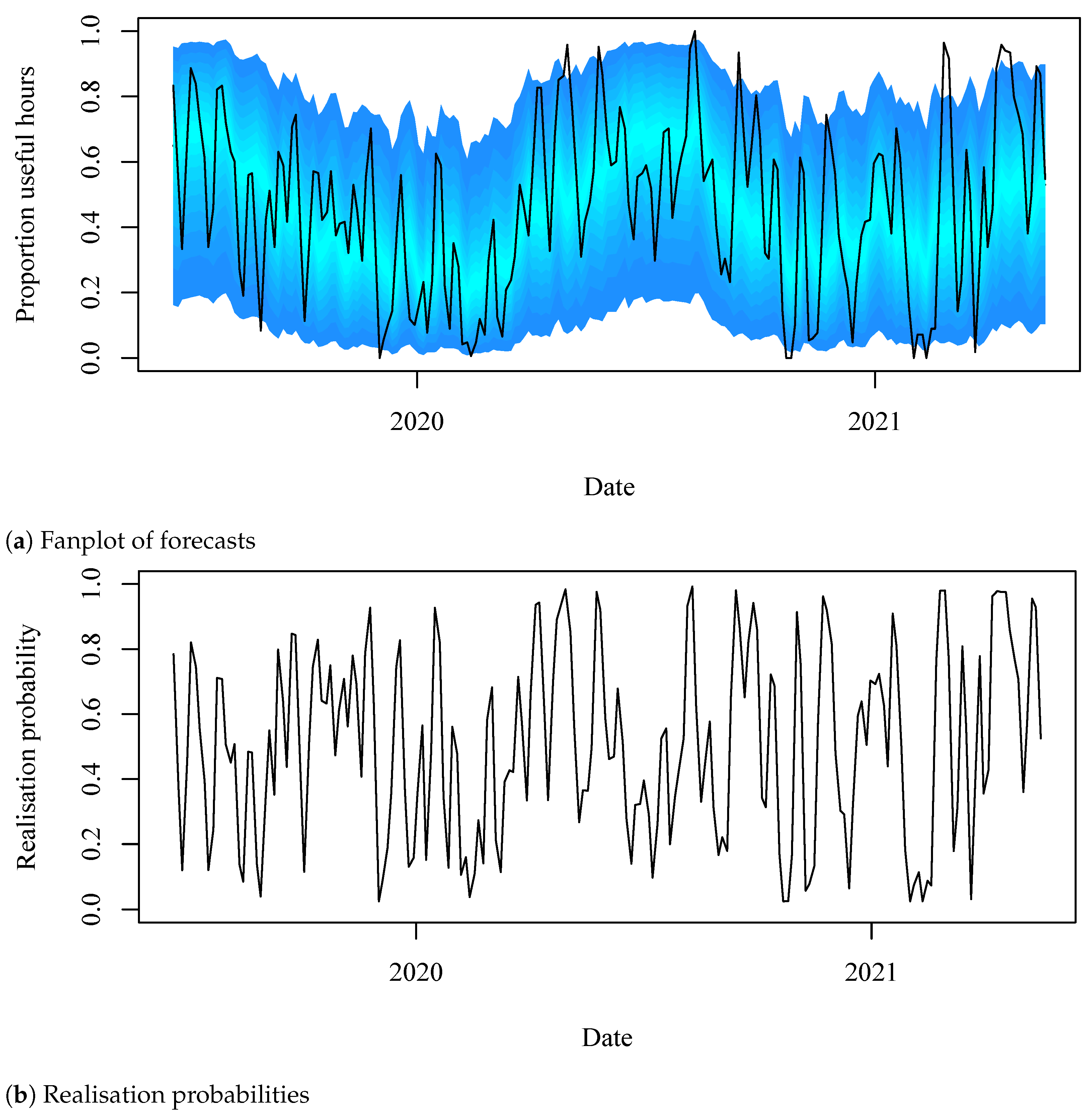
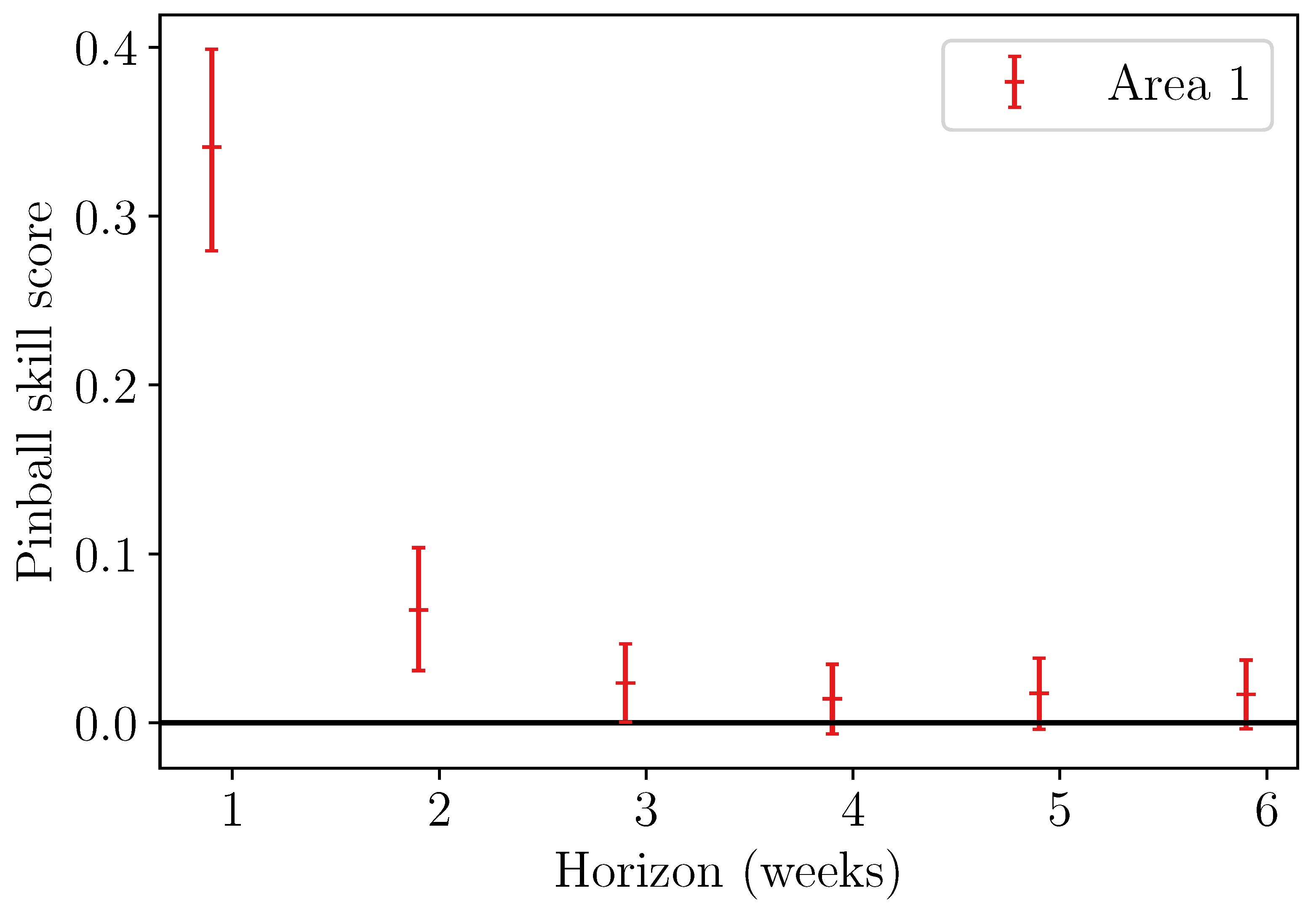
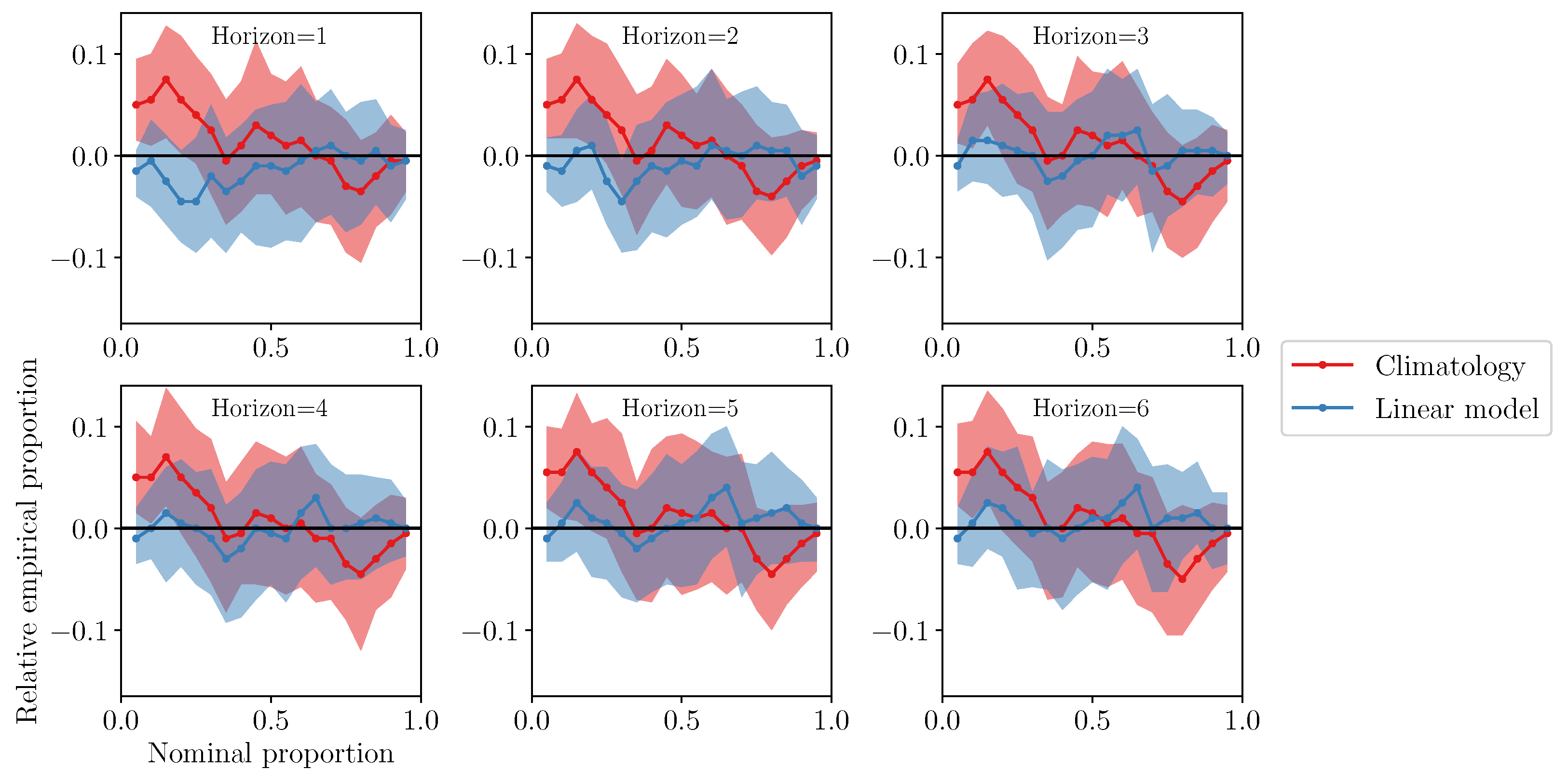
A fan plot of the weather window index (Figure 17) shows that the forecasts follow seasonal trends well and do also have some sensitivity to shorter-term spikes, although the forecast distribution is generally quite broad. The weather window index forecasts have very good skill at all sites for 1 week ahead, fair skill for 2–3 weeks ahead and some skill at most sites beyond that (Figure 18). All forecasts are calibrated across all horizons, with the exception of the 1 week ahead forecasts for the area 4 sites. Verification for WF1 is shown in Figure 19.
To perform a cost-loss calculation, the form of the losses incurred for the crane maintenance problem must be determined. It is assumed that any turbines that need to be fixed are currently not operational, so that losses consist of the lost energy whilst the turbine is down. Then, the expectation value of lost energy for the week can be calculated. An alternative assumption would be that the turbines can continue to operate before the repair, in which case lost energy is only incurred from the downtime while the repair takes place. The expected lost energy is given by
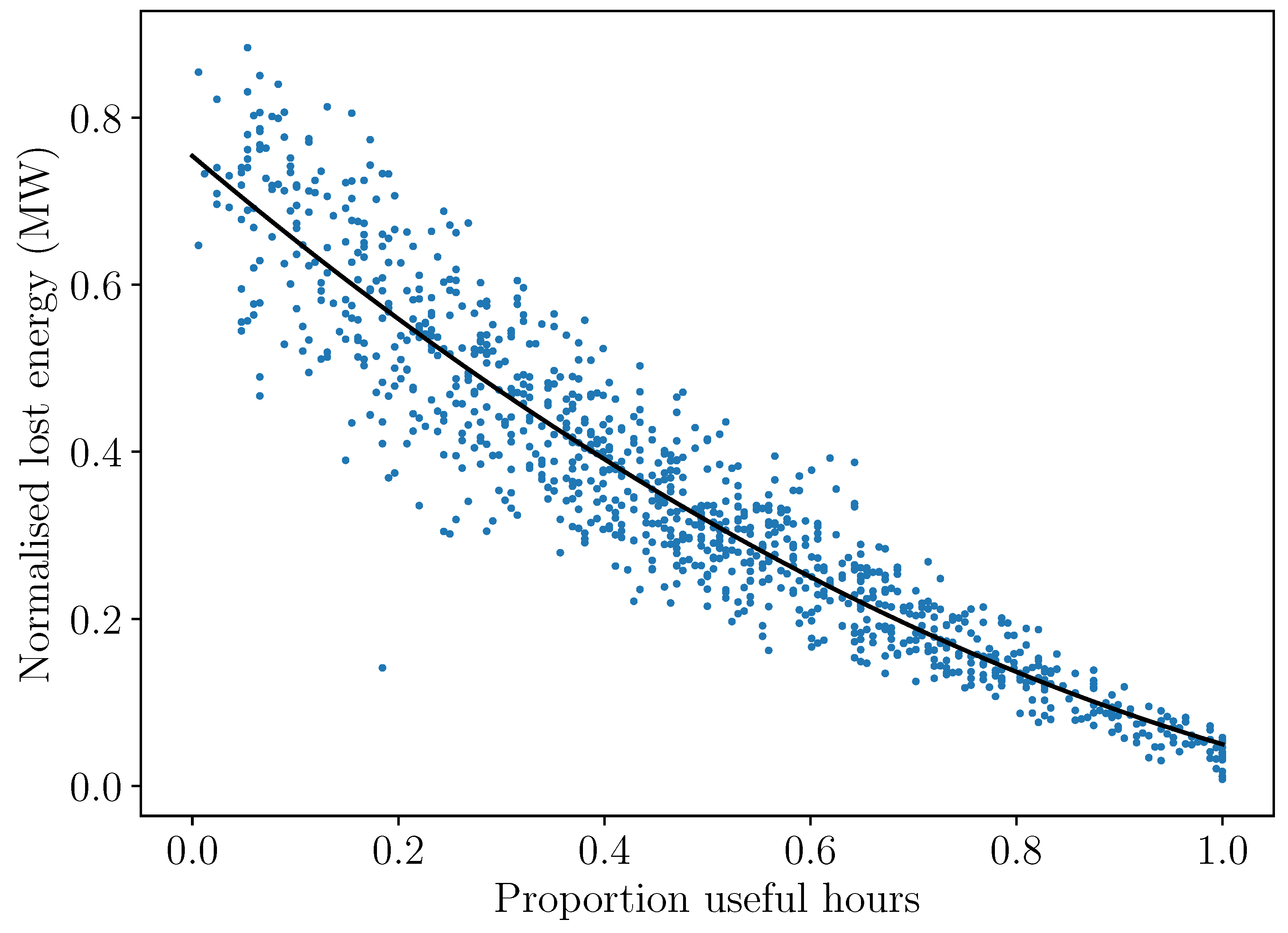
where x denotes the number of useful window hours in the week, is the loss function and is the forecast distribution. represents the losses incurred when a turbine is not fixed; in this case, this is assumed to be the value of lost energy. To calculate this, the hourly resolution site wind speeds are passed through a turbine power curve before being summed into a value for weekly lost energy per turbine. Figure 20 shows the relationship between the number of useful hours x and the lost energy for that week . This relationship is modelled as quadratic, so the loss function becomes
and the expected lost energy (Equation (20)) becomes
where is the beta distribution with parameters , and is the Dirac delta function centred at 0. Using the properties when or and the recursion relation for the beta function , Equation (22) evaluates to
Here, a, b and c are estimated from a quadratic fit to the relationship shown in Figure 20. , , and are the BEINF parameters estimated through GAMLSS model fitting following Equations (14)–(17) and are then converted to , , and using the relations in Equation (18).
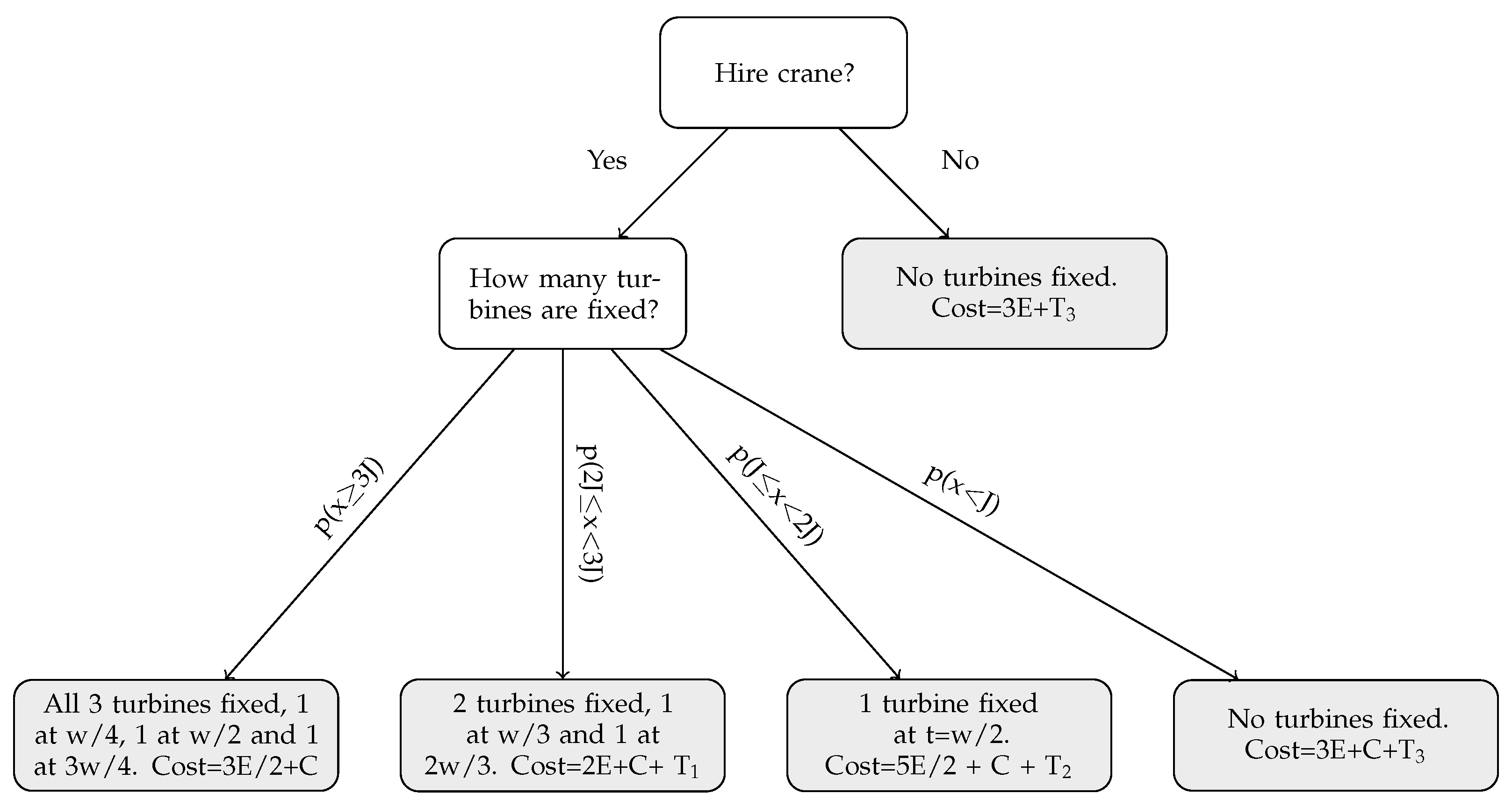
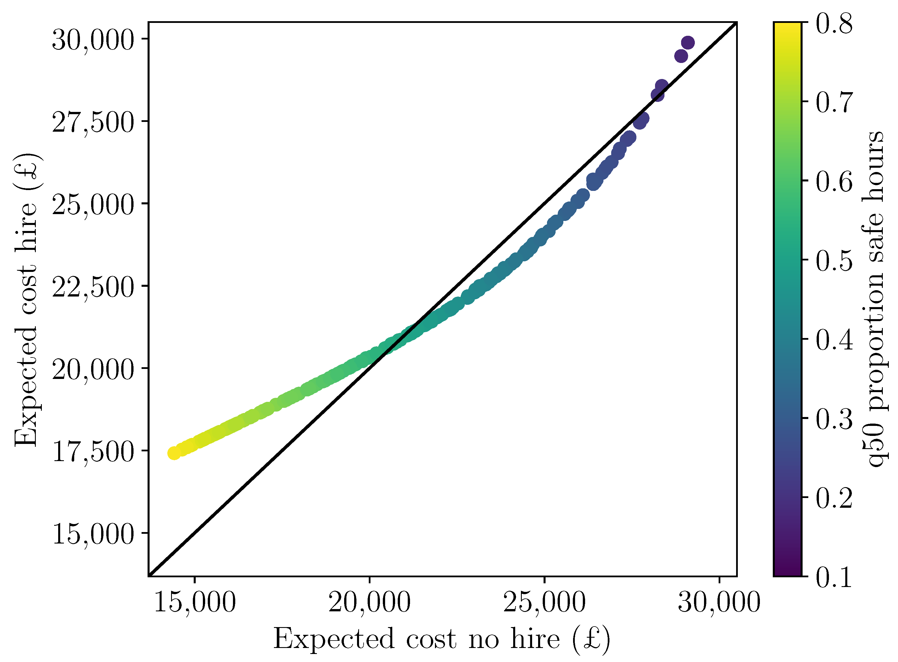
Figure 21 shows the various possible scenarios, given that three turbines need to be repaired. The expected cost from not hiring the crane includes the lost energy for the week plus a terminal penalty given by the average energy loss in subsequent weeks before the next opportunity to repair all remaining turbines. If a crane is hired, there are several different numbers of turbines that could be fixed depending on the actual weather conditions that week. The end cost of a scenario where n turbines are fixed and m turbines remain down is the cost of energy for the portion of the week before the n turbines are fixed, plus the lost energy for the entire week for the m turbines that are not fixed, plus the cost of the crane, plus a final terminal penalty of the average energy loss in subsequent weeks before the next opportunity to repair the m remaining turbines. The overall expected cost of hiring the crane is the sum of these scenarios, weighted by their probabilities of occurrence. These probabilities of occurrence are derived from the forecast distribution of x, the number of useful hours in the week. Then, a decision on whether to hire a crane may be made, based on which option has the lowest expected cost given the forecast. This decision is sensitive to two costs: the cost of crane hire and the cost of lost power production, which depends on the electricity price. The expected costs of hiring or not hiring are plotted in Figure 22. All points below the line represent times where hiring a crane is cheaper than not hiring one.
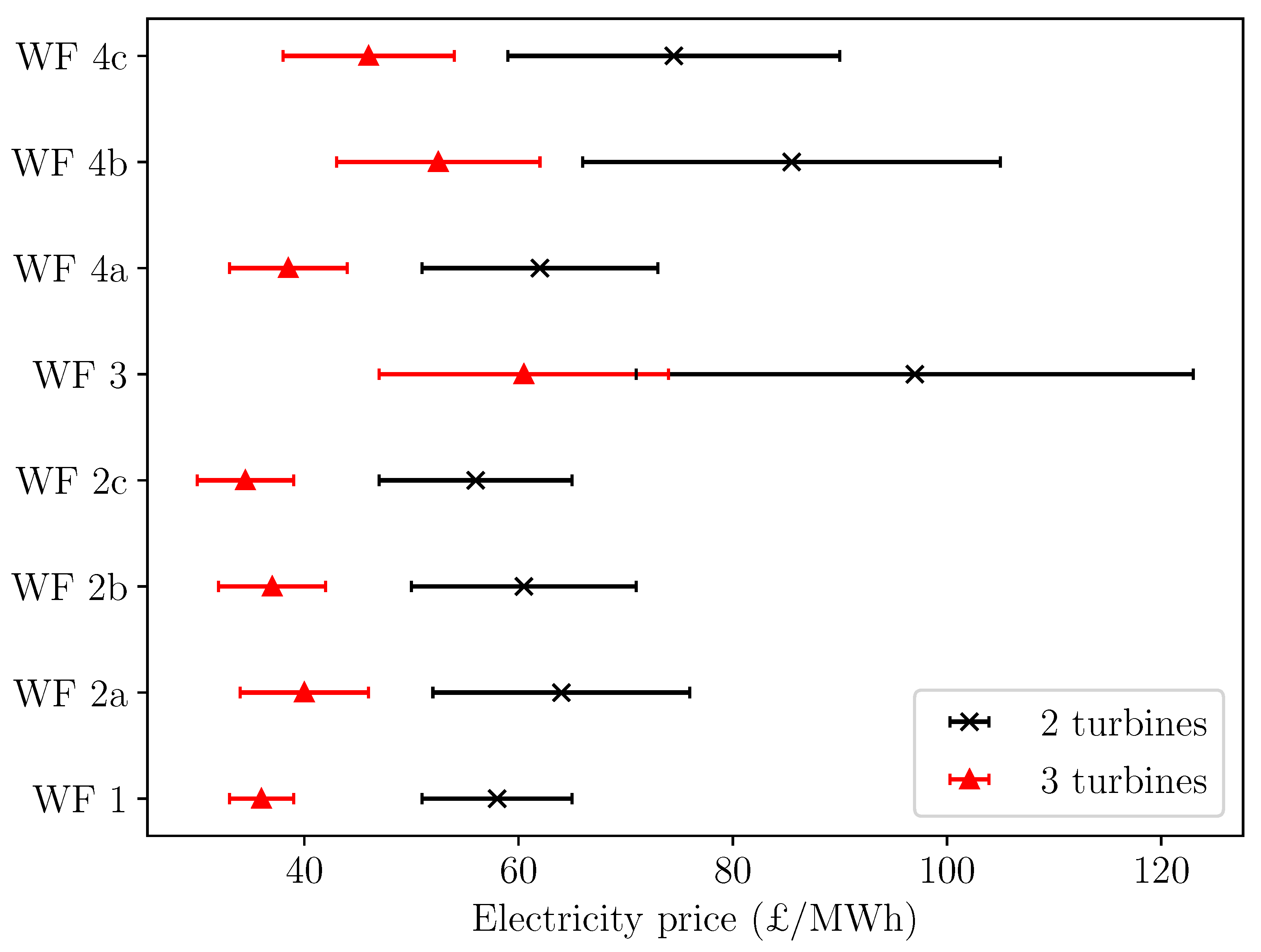
At very high electricity prices, the expected cost of lost energy is always greater than the expected costs incurred if a crane is hired (the curve in Figure 22 is shifted so that it lies entirely below the line), so the decision is always to hire the crane. Conversely, at very low electricity prices, the cost of lost energy is much less than the cost of the crane and so it is never beneficial to hire the crane. In reality, there may be other contractual penalties for failure to repair any turbines but this is not included in the cost-loss model used here, as the financial cost of this may be linked to the maintenance of the whole wind farm across a whole season rather than individual maintenance decisions. For the cost-loss model in this example, for a given crane hire cost, there exists a range of electricity prices, where the decision to hire or not hire depends on the forecast number of useful hours in the week (equally, for a set electricity price, there would be a range of crane hire prices where this also holds). The range of electricity prices where the decision to hire or not hire a crane is sensitive to the forecast number of useful hours is shown in Figure 23. Further analysis is based on WF3, where the range of electricity prices is the greatest.
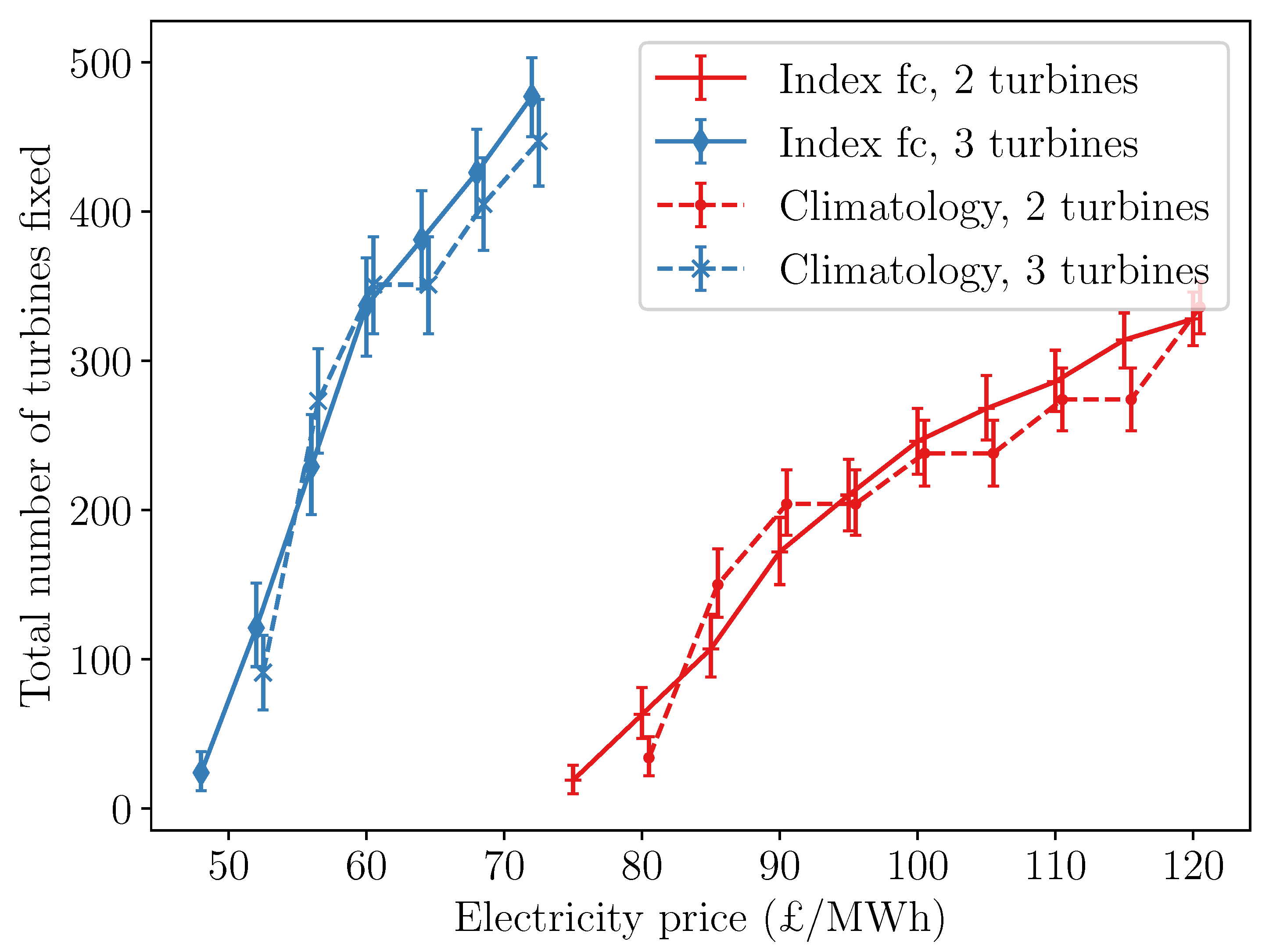
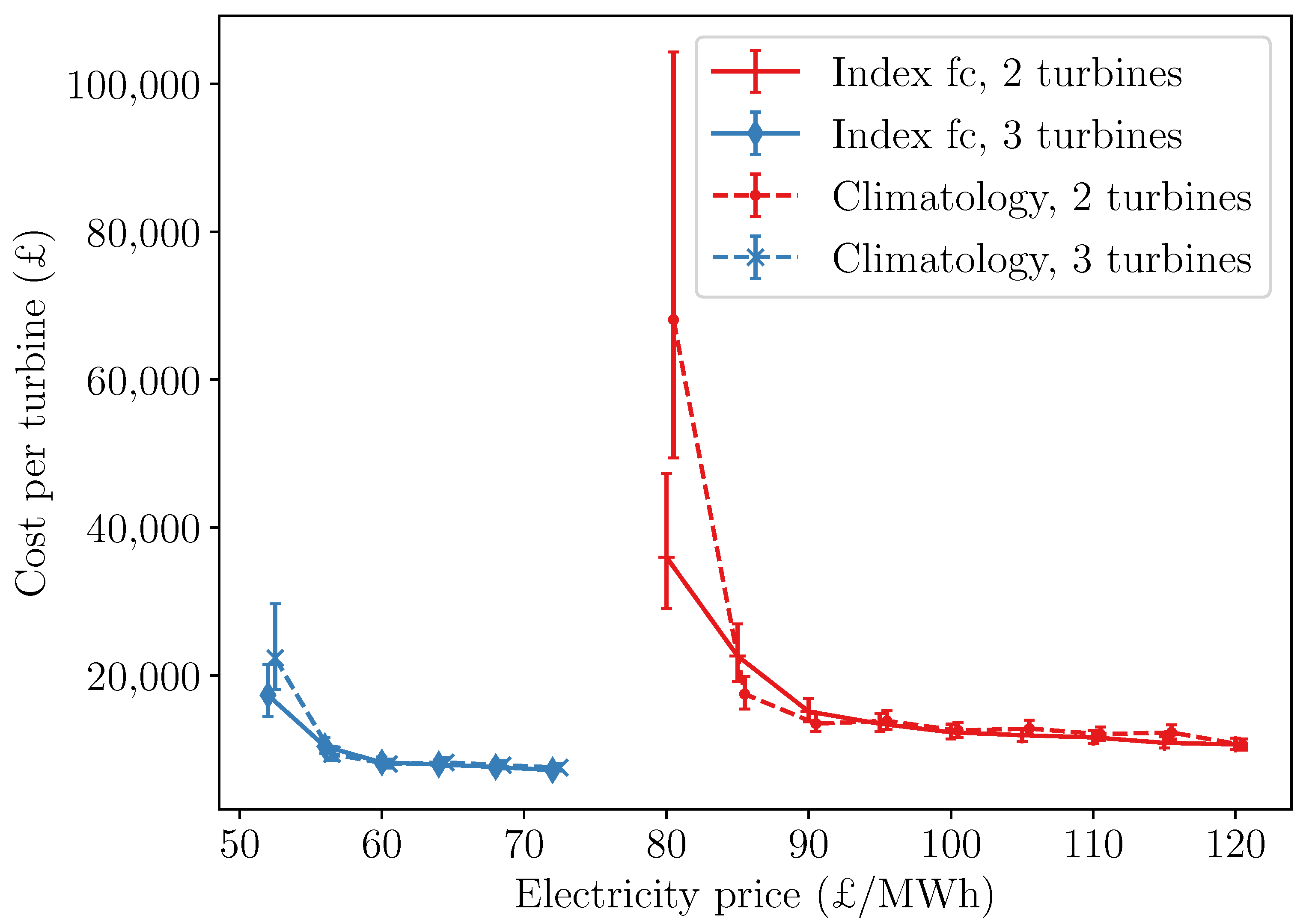
The true cost of crane hire decisions is evaluated by comparison to what the actual weather would have allowed. The number and timings of actual weather windows in the ERA5 site wind speed data give the first available times that each turbine may be fixed and the corresponding actual lost energy before those times. Then, the ‘actual’ cost of hiring or not hiring can be calculated. The total cost calculated assumes that there are always either two or three turbines down, across all 200 weeks evaluated. However, in reality, this scenario will only apply for a portion of weeks, and the more relevant metrics are the number of turbines fixed and the average cost per turbine. These metrics are shown in Table 2 and plotted in Figure 24 and Figure 25, respectively. As might be expected, the total number of turbines fixed increases with the electricity price as the decision to hire a crane is made a higher proportion of the time when the cost of lost energy is higher. There is no clear difference in the number of turbines fixed between decisions based on climatology or the S2S index forecasts. Again, there is little difference between climatology or S2S forecasts in cost per turbine, apart from at the lowest electricity price considered, where no turbines were fixed under climatology. Above £60/MWh for three turbines or £90/MWh for two turbines, the cost per turbine is relatively stable. Comparing the decisions made at each timestamp by the climatology or S2S index forecasts, both forecasts made the same hiring decision at 189 of the 200 weeks analysed, which perhaps explains why the costs associated with both forecasts are so similar.
4. Conclusions
Forecasts of weekly mean wind speed, weekly wind speed variation and number of useful work hours within the week have been shown to be skilful on S2S timescales. Mean wind speed forecasts showed skill out to three weeks ahead. Variability forecasts had lower skill for one or two week horizons, but retained fair skill out to 6 weeks ahead. A new ‘weather window index’ of the number of useful hours in a week was proposed to inform activity-specific decision making—for example, crane hire. These weather window index forecasts showed very good skill one week ahead and fair skill out to 6 weeks. A cost-loss model was implemented to determine the economic benefit of forecasts, but found little difference between the decisions made under climatology and the decisions made by the S2S forecasts.
Training forecasts on reanalysis data corrected to the site showed no significant worsening in forecast skill compared to forecasts trained on a long measured time series of MIDAS data. When correcting reanalysis data to site measurements, accounting for seasonal variations improves the corrected time series by 0.8%. Due to the lack of 100 m wind speed variable in the ECMWF S2S forecasts, several weather variables related to 100 m wind speed were used in place. Performing one principal component analysis on all these variables together had little effect on the final forecast skill but improved computation times by decreasing the number of model inputs. A linear model with regularisation was used to generate site-specific index forecasts at weekly resolution; including standard deviation, min and max of all principal components (the input features to this model) as well as mean gave no improvement in mean wind speed forecast but was included for variability forecasts. Index forecasts were generated for each ensemble member, before EMOS was applied to correct for the under-dispersion seen in the ensemble.
Original contributions of this work include:
- A comparison between forecasts generated with a complete measured time series and those using reanalysis data corrected with a limited history of site data. This bridges the gap between common methods for desk-based studies and those necessary to apply models to real-world sites.
- Determination of the skill of S2S forecasts across three different metrics that are relevant for maintenance planning.
- Implementation of a cost-loss model and investigation of the sensitivity of hiring decisions to electricity prices.
To further extend this work, it would be beneficial to investigate the performance of other models to produce the index forecasts, especially non-linear models such as GAMLSS or gradient boosted trees that can also learn interactions between input features. Besides the simple linear model used here or a polynomial regression approach [10], no other types of model have been explored for this purpose. Further feature engineering could also prove beneficial. Weather window index forecasts were only generated for one wind speed threshold and weather window length. The safe limit for work in the hub is much higher and therefore ‘unsafe’ times will form a much smaller proportion of the dataset in this case; it would be interesting to explore how this affects the skill of the weather window forecasts and how this translates to decision making. Additionally, whole-site servicing campaigns require many individual but possibly interdependent decisions to be made. Allowing the sharing of resources between sites also adds complexity, as well as opportunities for cost reduction that were not considered here. Whole-campaign planning would also lend itself more easily to the inclusion of contractual penalties in the cost-loss model. The calculation of expected lost energy could also be improved by modelling the relationship between useful hours and lost energy (Figure 20) as heteroscedastic, although a careful choice of distribution would be needed to evaluate the subsequent integration exactly without numeric integration.
Supplementary Materials
The following are available online at https://www.mdpi.com/article/10.3390/wind2020015/s1.
Author Contributions
Conceptualization, R.T., J.B. and D.M.; methodology, R.T. and J.B.; software, R.T.; validation, R.T.; formal analysis, R.T.; investigation, R.T.; data curation, R.T.; writing—original draft preparation, R.T.; writing—review and editing, R.T. and J.B.; visualization, R.T.; supervision, J.B. and D.M. All authors have read and agreed to the published version of the manuscript.
Funding
This research was funded by The Data Lab Innovation Centre with co-funding from Natural Power Consultants Ltd. through the Ph.D. studentship held by Rosemary Tawn.
Institutional Review Board Statement
Not applicable.
Informed Consent Statement
Not applicable.
Data Availability Statement
Restrictions apply to the availability of the site wind speed data and code manipulating these data. Data were obtained from Natural Power Consultants Ltd. and are archived at https://doi.org/10.15129/36db34ee-dcf9-494e-8953-fbcaae626c08 (accessed on 11 August 2021), ECMWF forecasts can be downloaded from https://apps.ecmwf.int/datasets/data/s2s (accessed on 11 August 2021) and the MIDAS station dataset description is available at https://catalogue.ceda.ac.uk/uuid954d743d1c07d1dd034c131935db54e0 (accessed on 11 August 2021), downloadable through the CEDA web processing UI https://ceda-wps-ui.ceda.ac.uk/ (accessed on 11 August 2021)) for research purposes.
Acknowledgments
The authors would like to thank Natural Power Consultants Ltd. for their support, and the reviewers and editors who helped improve this article.
Conflicts of Interest
The authors declare no conflict of interest. The funders had no role in the design of the study; in the collection, analyses, or interpretation of data; in the writing of the manuscript, or in the decision to publish the results.
Abbreviations
The following abbreviations are used in this manuscript:
| EA | East Atlantic |
| EAWR | East Atlantic Western Russia |
| ECMWF | European Centre for Medium-range Weather Forecasts |
| EMOS | Ensemble Model Output Statistics |
| GAM(LSS) | Generalised Additive Model (for Location, Scale and Shape) |
| LASSO | Least Absolute Shrinkage and Selection Operator |
| MIDAS | Met Office Integrated Data Archive System |
| MJO | Madden–Julian Oscillation |
| NAO | North Atlantic Oscillation |
| NWP | Numerical Weather Prediction |
| PCA | Principal Component Analysis |
| S2S | Subseasonal-to-Seasonal |
| S2S4E | Subseasonal-to-Seasonal Forecasting for Energy |
| SCA | Scandinavian Pattern |
References
- Soret, A.; Torralba, V.; Cortesi, N.; Christel, I.; Palma, L.; Manrique-Suñén, A.; Lledó, L.; González-Reviriego, N.; Doblas-Reyes, F.J. Sub-Seasonal to Seasonal Climate Predictions for Wind Energy Forecasting. J. Phys. Conf. Ser. 2019, 1222, 012009. [Google Scholar] [CrossRef]
- Lledó, L.; Torralba, V.; Soret, A.; Ramon, J.; Doblas-Reyes, F. Seasonal Forecasts of Wind Power Generation. Renew. Energy 2019, 143, 91–100. [Google Scholar] [CrossRef]
- White, C.J.; Domeisen, D.I.V.; Acharya, N.; Adefisan, E.A.; Anderson, M.L.; Aura, S.; Balogun, A.A.; Bertram, D.; Bluhm, S.; Brayshaw, D.J.; et al. Advances in the Application and Utility of Subseasonal-to-Seasonal Predictions. Bull. Am. Meteorol. Soc. 2021; Early online release. [Google Scholar] [CrossRef]
- White, C.J.; Carlsen, H.; Robertson, A.W.; Klein, R.J.T.; Lazo, J.K.; Kumar, A.; Vitart, F.; Coughlan de Perez, E.; Ray, A.J.; Murray, V.; et al. Potential Applications of Subseasonal-to-Seasonal (S2S) Predictions. Meteorol. Appl. 2017, 24, 315–325. [Google Scholar] [CrossRef]
- World Meteorological Organisation. Subseasonal-to-Seasonal Prediction Project. Available online: http://s2sprediction.net (accessed on 11 August 2021).
- Soret, A. Subseasonal-to-Seasonal Forecasting for Energy. Available online: http://s2s4e.eu (accessed on 11 August 2021).
- Orlov, A.; Sillmann, J.; Vigo, I. Better Seasonal Forecasts for the Renewable Energy Industry. Nat. Energy 2020, 5, 108–110. [Google Scholar] [CrossRef]
- Lledó, L.; Doblas-Reyes, F.J. Predicting Daily Mean Wind Speed in Europe Weeks Ahead from MJO Status. Mon. Weather Rev. 2020, 148, 3413–3426. [Google Scholar] [CrossRef]
- Lledó, L.; Cionni, I.; Torralba, V.; Bretonnière, P.A.; Samsó, M. Seasonal Prediction of Euro-Atlantic Teleconnections from Multiple Systems. Environ. Res. Lett. 2020, 15, 074009. [Google Scholar] [CrossRef]
- Alonzo, B.; Tankov, P.; Drobinski, P.; Plougonven, R. Probabilistic Wind Forecasting up to Three Months Ahead Using Ensemble Predictions for Geopotential Height. Int. J. Forecast. 2020, 36, 515–530. [Google Scholar] [CrossRef]
- Bloomfield, H.C.; Brayshaw, D.J.; Charlton-Perez, A.J. Characterizing the Winter Meteorological Drivers of the European Electricity System Using Targeted Circulation Types. Meteorol. Appl. 2020, 27, e1858. [Google Scholar] [CrossRef]
- Cortesi, N.; Torralba, V.; González-Reviriego, N.; Soret, A.; Doblas-Reyes, F.J. Characterization of European Wind Speed Variability Using Weather Regimes. Clim. Dyn. 2019, 53, 4961–4976. [Google Scholar] [CrossRef] [Green Version]
- Bloomfield, H.C.; Brayshaw, D.J.; Gonzalez, P.L.M.; Charlton-Perez, A. Sub-Seasonal Forecasts of Demand, Wind Power and Solar Power Generation for 28 European Countries. Earth Syst. Sci. Data 2021, 13, 2259–2274. [Google Scholar] [CrossRef]
- van der Wiel, K.; Bloomfield, H.C.; Lee, R.W.; Stoop, L.P.; Blackport, R.; Screen, J.A.; Selten, F.M. The Influence of Weather Regimes on European Renewable Energy Production and Demand. Environ. Res. Lett. 2019, 14, 094010. [Google Scholar] [CrossRef]
- Dalgic, Y.; Lazakis, I.; Dinwoodie, I.; McMillan, D.; Revie, M. Advanced Logistics Planning for Offshore Wind Farm Operation and Maintenance Activities. Ocean. Eng. 2015, 101, 211–226. [Google Scholar] [CrossRef] [Green Version]
- Lazakis, I.; Khan, S. An Optimization Framework for Daily Route Planning and Scheduling of Maintenance Vessel Activities in Offshore Wind Farms. Ocean. Eng. 2021, 225, 108752. [Google Scholar] [CrossRef]
- Shafiee, M. Maintenance Logistics Organization for Offshore Wind Energy: Current Progress and Future Perspectives. Renew. Energy 2015, 77, 182–193. [Google Scholar] [CrossRef]
- Taboada, J.V.; Diaz-Casas, V.; Yu, X. Reliability and Maintenance Management Analysis on Offshore Wind Turbines (OWTs). Energies 2021, 14, 7662. [Google Scholar] [CrossRef]
- Irawan, C.A.; Ouelhadj, D.; Jones, D.; Stålhane, M.; Sperstad, I.B. Optimisation of Maintenance Routing and Scheduling for Offshore Wind Farms. Eur. J. Oper. Res. 2017, 256, 76–89. [Google Scholar] [CrossRef] [Green Version]
- Barlow, E.; Tezcaner Öztürk, D.; Revie, M.; Boulougouris, E.; Day, A.H.; Akartunalı, K. Exploring the Impact of Innovative Developments to the Installation Process for an Offshore Wind Farm. Ocean. Eng. 2015, 109, 623–634. [Google Scholar] [CrossRef] [Green Version]
- Ji, G.; Wu, W.; Zhang, B. Robust Generation Maintenance Scheduling Considering Wind Power and Forced Outages. IET Renew. Power Gener. 2016, 10, 634–641. [Google Scholar] [CrossRef]
- Yu, Q.; Patriksson, M.; Sagitov, S. Optimal Scheduling of the next Preventive Maintenance Activity for a Wind Farm. arXiv 2020, arXiv:2001.03889. [Google Scholar] [CrossRef]
- Barlow, E.; Bedford, T.; Revie, M.; Tan, J.; Walls, L. A Performance-Centred Approach to Optimising Maintenance of Complex Systems. Eur. J. Oper. Res. 2021, 292, 579–595. [Google Scholar] [CrossRef]
- Pelajo, J.C.; Brandão, L.E.; Gomes, L.L.; Klotzle, M.C. Wind Farm Generation Forecast and Optimal Maintenance Schedule Model. Wind Energy 2019, 22, 1872–1890. [Google Scholar] [CrossRef]
- Browell, J.; Dinwoodie, I.; McMillan, D. Forecasting for Day-Ahead Offshore Maintenance Scheduling under Uncertainty. In Risk, Reliability and Safety: Innovating Theory and Practice; Walls, L., Revie, M., Bedford, T., Eds.; CRC Press: Boca Raton, FL, USA, 2016; pp. 1137–1144. [Google Scholar] [CrossRef] [Green Version]
- Vitart, F.; Ardilouze, C.; Bonet, A.; Brookshaw, A.; Chen, M.; Codorean, C.; Déqué, M.; Ferranti, L.; Fucile, E.; Fuentes, M.; et al. The Subseasonal to Seasonal (S2S) Prediction Project Database. Bull. Am. Meteorol. Soc. 2017, 98, 163–173. [Google Scholar] [CrossRef]
- Wiser, R.; Bolinger, M.; Hoen, B.; Millstein, D.; Rand, J.; Barbose, G.; Darghouth, N.; Gorman, W.; Jeong, S.; Mills, A.; et al. Land-Based Wind Market Report: 2021 Edition; Technical Report; US Department for Energy: Washington, DC, USA, 2021.
- Met Office. Met Office Integrated Data Archive System (MIDAS) Land and Marine Surface Stations Data (1853–Current). 2012. Available online: http://catalogue.ceda.ac.uk/uuid/220a65615218d5c9cc9e4785a3234bd0 (accessed on 11 August 2021).
- Ramon, J.; Lledó, L.; Torralba, V.; Soret, A.; Doblas-Reyes, F.J. What Global Reanalysis Best Represents Near-surface Winds? Q. J. R. Meteorol. Soc. 2019, 145, 3236–3251. [Google Scholar] [CrossRef] [Green Version]
- Schuhen, N.; Thorarinsdottir, T.L.; Gneiting, T. Ensemble Model Output Statistics for Wind Vectors. Mon. Weather Rev. 2012, 140, 3204–3219. [Google Scholar] [CrossRef] [Green Version]
- Rigby, R.A.; Stasinopoulos, D.M. Generalized Additive Models for Location, Scale and Shape. Appl. Stat. 2005, 54, 507–554. [Google Scholar] [CrossRef] [Green Version]
- Scheuerer, M. Probabilistic Quantitative Precipitation Forecasting Using Ensemble Model Output Statistics: Probabilistic Precipitation Forecasting Using EMOS. Q. J. R. Meteorol. Soc. 2014, 140, 1086–1096. [Google Scholar] [CrossRef] [Green Version]
Figure 1.
Flowchart of data and modelling steps to produce the final site index forecasts. The Principal Component Analysis step identifies large-scale weather patterns in the grid of forecasts over a whole European and North Atlantic area; the ERA5 correction to site fits a Generalised Additive Model (GAM) to correct ERA5 wind speeds to more closely match the short history of observed site wind speeds. The site index model takes the S2S principal components as inputs and is trained to forecast a site-specific index given by the site data for the training set. The Ensemble Model Output Statistics step corrects any bias or dispersion problems with the ensemble of site index forecasts before forecasts are evaluated.

Figure 2.
ERA5 windspeeds compared to site wind speeds before and after correction. Shown for WF1.

Figure 3.
Principal components of 500 hPa geopotential height mapped back to geographical space, for January and July.
Figure 3.
Principal components of 500 hPa geopotential height mapped back to geographical space, for January and July.

Figure 4.
Weekly mean wind speed index forecast versus observed weekly mean forecast, for 2 weeks ahead forecasts at the MIDAS 4 station.
Figure 4.
Weekly mean wind speed index forecast versus observed weekly mean forecast, for 2 weeks ahead forecasts at the MIDAS 4 station.

Figure 5.
Time series of all individual ensemble member 2 weeks ahead index forecasts (light grey), overlaid with the actual weekly mean wind speeds (black). There is clear under-dispersion in the set of ensemble members.
Figure 5.
Time series of all individual ensemble member 2 weeks ahead index forecasts (light grey), overlaid with the actual weekly mean wind speeds (black). There is clear under-dispersion in the set of ensemble members.

Figure 6.
Verification rank histogram of all 2 weeks ahead ensemble member index forecasts, showing the ‘U’ shape characteristic of under-dispersion.
Figure 6.
Verification rank histogram of all 2 weeks ahead ensemble member index forecasts, showing the ‘U’ shape characteristic of under-dispersion.

Figure 7.
Pinball skill score of weekly mean wind speed index, at MIDAS 1 and relative to climatology. The three index model configurations are with separate Principal Components, with extra weekly features (standard deviation, min and max) of the PCs inputs, and where all 100 m weather variables are transformed into PCs together. Error bars show 95% bootstrapped confidence intervals.

Figure 8.
Normalised reliability diagram for mean wind speed index and the equivalent climatology forecast, at MIDAS 1. The forecast labelled ‘linear model’ is calculated with separate PCs and no extra engineered features. Horizons are in number of weeks.
Figure 8.
Normalised reliability diagram for mean wind speed index and the equivalent climatology forecast, at MIDAS 1. The forecast labelled ‘linear model’ is calculated with separate PCs and no extra engineered features. Horizons are in number of weeks.

Figure 9.
Pinball skill score of weekly mean wind speed index relative to climatology. The forecasts labelled ‘WF 1’ are based on corrected ERA5 data for that wind farm. Error bars show 95% bootstrapped confidence intervals. MIDAS skill score is calculated relative to climatology of the MIDAS wind speed data and WF1 skill score is calculated relative to climatology of the corrected ERA5 data.

Figure 10.
Reliability of weekly mean wind speed forecast at MIDAS 1. Intervals show 95% bootstrapped confidence bands.
Figure 10.
Reliability of weekly mean wind speed forecast at MIDAS 1. Intervals show 95% bootstrapped confidence bands.

Figure 11.
Reliability of weekly mean wind speed forecast at WF1. Intervals show 95% bootstrapped confidence bands.
Figure 11.
Reliability of weekly mean wind speed forecast at WF1. Intervals show 95% bootstrapped confidence bands.

Figure 12.
Pinball skill score of weekly mean wind speed index relative to climatology at WF 1, across the forecast distribution. The two week ahead forecast is shown here. Coloured band shows the 95% bootstrapped confidence interval.
Figure 12.
Pinball skill score of weekly mean wind speed index relative to climatology at WF 1, across the forecast distribution. The two week ahead forecast is shown here. Coloured band shows the 95% bootstrapped confidence interval.

Figure 13.
Scatter plots of realisation probabilities for neighbouring sites. The solid black line shows , i.e., perfect correlation in realisation probabilities, where the two sites are always under- or overforecast by the same proportion at the same times.
Figure 13.
Scatter plots of realisation probabilities for neighbouring sites. The solid black line shows , i.e., perfect correlation in realisation probabilities, where the two sites are always under- or overforecast by the same proportion at the same times.

Figure 14.
Pinball skill score of weekly variability (weekly standard deviation of hourly wind speeds) relative to climatology. The forecasts labelled ‘WF 1’ are based on corrected ERA5 data for that wind farm. Error bars show 95% bootstrapped confidence intervals.
Figure 14.
Pinball skill score of weekly variability (weekly standard deviation of hourly wind speeds) relative to climatology. The forecasts labelled ‘WF 1’ are based on corrected ERA5 data for that wind farm. Error bars show 95% bootstrapped confidence intervals.

Figure 15.
Reliability of variability forecast at MIDAS 1. Intervals show 95% bootstrapped confidence bands.
Figure 15.
Reliability of variability forecast at MIDAS 1. Intervals show 95% bootstrapped confidence bands.

Figure 16.
Reliability of variability forecast at WF1. Intervals show 95% bootstrapped confidence bands.
Figure 16.
Reliability of variability forecast at WF1. Intervals show 95% bootstrapped confidence bands.

Figure 17.
(a) Fan plot of 2 weeks ahead weather window index forecasts. (b) Time series of realisation probabilities for the same forecasts as (a).
Figure 17.
(a) Fan plot of 2 weeks ahead weather window index forecasts. (b) Time series of realisation probabilities for the same forecasts as (a).

Figure 18.
Pinball skill score of weather window index relative to climatology for area 1. Error bars show 95% bootstrapped confidence intervals.
Figure 18.
Pinball skill score of weather window index relative to climatology for area 1. Error bars show 95% bootstrapped confidence intervals.

Figure 19.
Reliability of weather window index forecast at WF1. Intervals show 95% bootstrapped confidence bands.
Figure 19.
Reliability of weather window index forecast at WF1. Intervals show 95% bootstrapped confidence bands.

Figure 20.
Relationship between number of hours in a weather window and weekly total lost energy at WF1. Both axes are normalised by their maximum (i.e., number of hours in a week and maximum weekly energy output).
Figure 20.
Relationship between number of hours in a weather window and weekly total lost energy at WF1. Both axes are normalised by their maximum (i.e., number of hours in a week and maximum weekly energy output).

Figure 21.
Flowchart of crane hire decision and resulting costs, assuming that three turbines are broken. The week starts at time t = 0 and ends at time t = w. E is the expected cost of lost energy for one turbine for the whole week, given the weather window index forecast (see Equations (20)–(23)). C denotes the cost of crane hire for the week, J denotes the job time for repair of one turbine and T is a terminal cost representing the average energy loss in subsequent weeks before the next opportunity to repair the m unfixed turbines. x is the number of useful hours. Where one or more turbines are repaired, the times of repair are assumed to be divided evenly throughout the week.

Figure 22.
Expected cost of hiring crane vs. expected cost of not hiring crane, for 2 weeks ahead forecasts of number of available hours in the week. Colour shows the q50 forecast value of normalised number of hours within a weather window.
Figure 22.
Expected cost of hiring crane vs. expected cost of not hiring crane, for 2 weeks ahead forecasts of number of available hours in the week. Colour shows the q50 forecast value of normalised number of hours within a weather window.

Figure 23.
Range of electricity prices at each site, where crane hire decision is sensitive to the forecast number of weather window hours, for either 2 or 3 turbines down. Marker shows the median price and whiskers show the minimum and maximum electricity prices where the hire decision is sensitive to the forecast.

Figure 24.
Number of turbines fixed when index forecasts or climatology forecasts are used to make crane hiring decision, dependent on electricity price, at WF3. Error bars show 95% bootstrapped confidence intervals.
Figure 24.
Number of turbines fixed when index forecasts or climatology forecasts are used to make crane hiring decision, dependent on electricity price, at WF3. Error bars show 95% bootstrapped confidence intervals.

Figure 25.
Cost of crane hire and lost energy when index forecasts or climatology forecasts are used to make hiring decision, for a range of electricity prices, at WF3. Error bars show 95% bootstrapped confidence intervals.
Figure 25.
Cost of crane hire and lost energy when index forecasts or climatology forecasts are used to make hiring decision, for a range of electricity prices, at WF3. Error bars show 95% bootstrapped confidence intervals.


Table 1.
Table of index model input features. gph = geopotential height; ws = wind speed. * 925 and 1000 hPa wind speed and mean sea level pressure are all included in one PC transform together.
Table 1.
Table of index model input features. gph = geopotential height; ws = wind speed. * 925 and 1000 hPa wind speed and mean sea level pressure are all included in one PC transform together.
| Variable (s) | PCs Kept | Features | Index Models | ||
|---|---|---|---|---|---|
| Mean ws | Variability | Weather Window | |||
| weekly mean | √ | √ | √ | ||
| 500 hPa gph | 20 | weekly sd | √ | ||
| weekly min, max | √ | ||||
| weekly mean | √ | √ | √ | ||
| 10 m ws | 40 | weekly sd | √ | ||
| weekly min, max | √ | ||||
| weekly mean | √ | √ | √ | ||
| 100 m variables * | 20 | weekly sd | √ | ||
| weekly min, max | √ | ||||
Table 2.
Results of cost-loss analysis for a range of electricity prices at WF3, for the 2 weeks ahead forecasts. The cost per turbine includes both crane hire cost and the cost of lost energy before turbines were fixed. Number of turbines fixed is assuming ‘N turbines down’ needed repair for every week in the 2-year forecast period.
| N Turbines Down | Electricity Price £/MWh | N Fixed (Index Model) | £/Turbine (Index Model) | N Fixed (Climatology) | £/Turbine (Climatlogy) |
|---|---|---|---|---|---|
| 2 | 75 | 19 | 110,900 | 0 | - |
| 2 | 80 | 63 | 35,980 | 34 | 68,090 |
| 2 | 85 | 107 | 22,610 | 150 | 17,470 |
| 2 | 90 | 172 | 15,100 | 204 | 13,480 |
| 2 | 95 | 210 | 13,450 | 204 | 13,830 |
| 2 | 100 | 246 | 12,300 | 238 | 12,530 |
| 2 | 105 | 268 | 11,890 | 238 | 12,800 |
| 2 | 110 | 286 | 11,600 | 274 | 12,050 |
| 2 | 115 | 314 | 10,860 | 274 | 12,270 |
| 2 | 120 | 328 | 10,660 | 336 | 10,580 |
| 3 | 48 | 24 | 73,300 | 0 | - |
| 3 | 52 | 121 | 17,320 | 91 | 22,340 |
| 3 | 56 | 229 | 10,380 | 273 | 9330 |
| 3 | 60 | 337 | 8220 | 351 | 8000 |
| 3 | 64 | 381 | 7940 | 351 | 8200 |
| 3 | 68 | 426 | 7608 | 405 | 7850 |
| 3 | 72 | 477 | 7170 | 447 | 7520 |
Publisher’s Note: MDPI stays neutral with regard to jurisdictional claims in published maps and institutional affiliations. |
© 2022 by the authors. Licensee MDPI, Basel, Switzerland. This article is an open access article distributed under the terms and conditions of the Creative Commons Attribution (CC BY) license (https://creativecommons.org/licenses/by/4.0/).
Share and Cite
MDPI and ACS Style
Tawn, R.; Browell, J.; McMillan, D. Subseasonal-to-Seasonal Forecasting for Wind Turbine Maintenance Scheduling. Wind 2022, 2, 260-287. https://doi.org/10.3390/wind2020015
AMA Style
Tawn R, Browell J, McMillan D. Subseasonal-to-Seasonal Forecasting for Wind Turbine Maintenance Scheduling. Wind. 2022; 2(2):260-287. https://doi.org/10.3390/wind2020015
Chicago/Turabian StyleTawn, Rosemary, Jethro Browell, and David McMillan. 2022. "Subseasonal-to-Seasonal Forecasting for Wind Turbine Maintenance Scheduling" Wind 2, no. 2: 260-287. https://doi.org/10.3390/wind2020015