the Creative Commons Attribution 4.0 License.
the Creative Commons Attribution 4.0 License.
 | 22 Mar 2018
Simultaneous 6300 Å airglow and radar observations of ionospheric irregularities and dynamics at the geomagnetic equator
Carlos R. Martinis
Michael Mendillo
Jeffrey Baumgardner
Joei Wroten
Marco Milla
In March 2014 an all-sky imager (ASI) was installed at the Jicamarca Radio Observatory (11.95∘ S, 76.87∘ W; 0.3∘ S MLAT). We present results of equatorial spread F (ESF) characteristics observed at Jicamarca and at low latitudes. Optical 6300 and 7774 Å airglow observations from the Jicamarca ASI are compared with other collocated instruments and with ASIs at El Leoncito, Argentina (31.8∘ S, 69.3∘ W; 19.8∘ S MLAT), and Villa de Leyva, Colombia (5.6∘ N, 73.52∘ W; 16.4∘ N MLAT). We use Jicamarca radar data, in incoherent and coherent modes, to obtain plasma parameters and detect echoes from irregularities. We find that ESF depletions tend to appear in groups with a group-to-group separation around 400–500 km and within-group separation around 50–100 km. We combine data from the three ASIs to investigate the conditions at Jicamarca that could lead to the development of high-altitude, or topside, plumes. We compare zonal winds, obtained from a Fabry–Pérot interferometer, with plasma drifts inferred from the zonal motion of plasma depletions. In addition to the ESF studies we also investigate the midnight temperature maximum and its effects at higher latitudes, visible as a brightness wave at El Leoncito. The ASI at Jicamarca along with collocated and low-latitude instruments provide a clear two-dimensional view of spatial and temporal evolution of ionospheric phenomena at equatorial and low latitudes that helps to explain the dynamics and evolution of equatorial ionospheric/thermospheric processes.
Keywords. Ionosphere (equatorial ionosphere; ionospheric irregularities; plasma temperature and density)
- Article
(10041 KB) -
Supplement
(6681 KB) - BibTeX
- EndNote


All-sky imagers (ASIs) at equatorial and low latitudes are used to study thermospheric and ionospheric processes like equatorial spread F (ESF) and the brightness wave (BW), a consequence of the midnight temperature maximum (MTM). Equatorial spread F refers to plasma irregularities that occur after sunset in the equatorial and low-latitude F region (Woodman and La Hoz, 1976). The MTM is an increase in neutral temperature that occurs in the thermosphere around local midnight (Spencer et al., 1979). Equatorial spread F has significant impacts on space weather such as disrupting navigation and communications signals through scintillation (Kintner et al., 2001) and the temporal and spatial variations of the MTM help to describe the role that lower atmospheric tides have on the upper atmosphere (Akmaev et al., 2009).
After sunset, the main radar at the Jicamarca Radio Observatory (50 MHz; 11.95∘ S, 76.87∘ W; 0.3∘ S MLAT) in Peru measures irregularities associated with ESF (Farley et al., 1970). The radar detects irregularities with scale sizes equal to half the radar wavelength (3 m). Large-scale ESF structures (10–500 km) can also be observed as airglow depletions within the field of view of ASIs (Weber et al., 1978). These structures are regions that have less plasma and thus are darker than the background. Depletions can be associated with three types of ESF: bottom-type, bottomside, and topside (Woodman and La Hoz, 1976). The large-scale structures of topside ESF are often referred to as plumes or plasma bubbles. At the magnetic equator we observe bottomside ESF that appears as dark bands oriented along magnetic field lines. Observations away from the magnetic equator measure topside ESF and are visible as bifurcated structures extending away from the magnetic equator. Equatorial spread F processes are flux-tube integrated (e.g., Sultan, 1996; Weber et al., 1996; Keskinen et al., 1998) so the topside structures at the magnetic equator map down to their magnetic foot points at higher latitudes (e.g., Mendillo and Baumgardner, 1982). The spectrum of ESF irregularities involves small and large scales. Small-scale irregularities are related to larger-scale size structures, although the production mechanism for some small-scale irregularities is not fully understood. It is often assumed that a cascade mechanism is responsible for the smaller-scale irregularities but the exact process is still debated (Woodman, 2009). Another explanation for the small-scale irregularities may be that the large-scale plumes create favorable conditions for small-scale instabilities to form. Hickey et al. (2015) postulated that the conditions for the lower hybrid drift instability, which can produce 0.34 m irregularities, and the gradient drift instability, which can produce 0.34 and 3 m irregularities, are met in certain regions of the depletions.
The imaging science team at Boston University operates a network of ASIs that are used for ESF observations in addition to many other science topics (Martinis et al., 2017). Observations of depletions with the ASI at the magnetic equator are the result of bottomside ESF because airglow emissions at 6300 Å typically come from an altitude that is about one neutral scale height (about 50 km) below the peak of the F layer. This is typically at an altitude of about 250 km a few hours after sunset at Jicamarca. ASIs at other sites at a similar longitude that are farther away from the magnetic equator are able to detect structures that extend into the topside of the ionosphere. These ASIs observe the footpoints of magnetic field lines that map to apex altitudes that are higher than the ASI observations at the magnetic equator (250 km). Bottomside ESF structures at Jicamarca do not always evolve into topside plumes (e.g., Hysell, 2000). In this study we compare observations at the magnetic equator with concurrent observations at nearby latitudes to investigate the evolution of bottomside structures to topside depletions.
One of the topics related to ESF that we discuss in this paper is the morphology of bottomside plasma depletions at the magnetic equator. Specifically, we are interested in measuring the zonal separation of airglow depletions to investigate how background conditions may modulate ESF. A study by Tsunoda and White (1981) showed that a 400 km large-scale wave structure (LSWS) modulated the production of ESF. They used coherent radar scans and found that ESF plumes formed at the crests of an LSWS. Since then, other studies have also found a connection between LSWS and the formation of ESF (e.g., Huang and Kelley, 1996; Narayanan et al., 2012; Patra et al., 2013; Joshi, 2016). Additionally, the distance between plasma depletions associated with ESF has been measured during solar minimum using imagers in Chile (Makela et al., 2010), Christmas Island, and Brazil (Chapagain et al., 2011). They both measured the spacing between adjacent plasma depletions and found that the structures were typically separated by 100–300 km. The observations from Makela et al. (2010) were interpreted as being the result of gravity waves but they do not discuss LSWSs.
In addition to studying the modulation of ESF, airglow observations of the zonal motion of ESF depletions can be used to infer zonal background plasma drifts. We are able to determine the plasma drifts by tracking the motion of plasma depletions with time. This is compared with concurrent measurements of the neutral wind using a collocated Fabry–Perot interferometer (FPI), helping to explain the connection between ions and neutrals in the upper atmosphere.
Another equatorial phenomenon we discuss in this paper, the MTM, has been studied directly using a variety of instruments such as satellites, incoherent scatter radars (ISR), and FPIs, (Herrero and Spencer, 1982; Hickey et al., 2014; Meriwether et al., 2008). At Jicamarca, the ISR has been used to study the seasonal dependence of the MTM (Bamgboye and McClure, 1982) and the MTM has been observed with FPIs at locations near the magnetic equator (Meriwether et al., 2008; Fisher et al., 2015). A signature of the MTM, known as a brightness wave, can be observed using an ASI. Colerico et al. (1996) reported the first BW detection with an ASI. A pressure bulge created by the MTM results in a reversal of meridional neutral wind, and this poleward wind drags the plasma with it (e.g., Colerico et al., 1996; Akmaev et al., 2010). Away from the magnetic equator the plasma moves downward along magnetic field lines as it is dragged by neutral species. As plasma moves down increased 6300 Å emission moving poleward in the field of view of the ASI is observed (i.e., a brightness wave). The brightness wave has been observed away from the magnetic equator at various latitudes and longitudes (e.g., Colerico et al., 1996; Fesen, 1996; Martinis et al., 2006).
In this paper our primary objective is to use the Jicamarca ASI and the suite of collocated instruments to explore depletion patterns and morphology and F region dynamics associated with ESF. In addition, we investigate how topside and bottomside ESF structures are connected. We also use these instruments to better understand the connection between the brightness wave and the MTM.
The Boston University ASI was installed at the Jicamarca Radio Observatory (JRO) in March 2014. In addition to the large ISR, there is a suite of instruments that includes other radars, an FPI, a magnetometer, and an ionosonde. The Jicamarca ASI takes images with four filters: three narrow band filters at 5577, 7774, and 6300 Å, and a cutoff filter of > 6950 Å. Each filter is used to observe different processes in the upper atmosphere that produce airglow emissions. Additionally there is a filter at 6050 Å that has no emission lines and is used for calibration purposes. The images taken with this filter are referred to as the background images. Emissions at 6300 and 7774 Å are well known to be related to ESF plasma signatures (Mendillo et al., 1985). In this work we focus on 6300 Å emission patterns. Emission of 6300 Å is due to a two-step process involving the dissociative recombination of O and electrons, followed by the de-excitation of atomic oxygen produced in that process. Thus, 6300 Å emission depends on electron density and the height of the ionospheric layer, which influences quenching (collisional de-excitation). Peak emission typically occurs between 250 and 300 km and is limited to a 50 km altitude range. However, at the magnetic equator, the emission layer can sometimes be as high as 400 km just after sunset. The other emission used to study the ionosphere is 7774 Å, which is caused by the radiative recombination of O+, and is directly proportional to total electron content. The majority of 7774 Å emission typically originates in the 300–400 km altitude range.
Two other ASIs, in El Leoncito, Argentina (31.8∘ S, 69.3∘ W; 19.6∘ S MLAT), and Villa de Leyva, Colombia (5.6∘ N, 73.52∘ W; 16.4∘ N MLAT), are used in this study to investigate topside plumes. The Villa de Leyva and El Leoncito ASIs are located such that they are at approximately magnetic conjugate points. The El Leoncito ASI is also used in the investigation of the MTM effects. Figure 1 shows the fields of view of the three ASIs for an 80∘ zenith angle at 250 km.
The Jicamarca ASI runs every night, except for a few nights around full moon, from sunset to sunrise. We have 517 nights of data available from 2014 to 2015 during solar maximum. The 10.7 cm solar radio flux during this time ranged from 100 to 150 solar flux units. During 120 nights we were able to observe plasma depletions associated with bottomside ESF. Ten nights showed no ESF depletions and the rest of the nights are inconclusive about ESF due to cloud cover. Figure 2 shows an example of raw (left) and unwarped (right) all-sky images taken at the Jicamarca Radio Observatory on 3 April 2014.
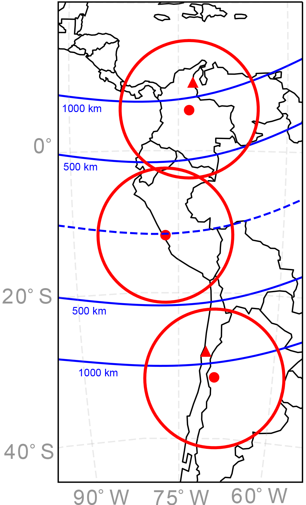
Figure 1A map of western South America showing the location of the Villa de Leyva (top), Jicamarca (middle), and El Leoncito (bottom) ASIs as red dots. The red circles around the dots are the fields of view for an airglow layer at 250 km and a zenith angle of 80∘. The red triangle in the Villa de Leyva field of view is the conjugate location of the El Leoncito ASI. The red triangle in the El Leoncito field of view is the conjugate location of the Villa de Leyva ASI. The blue dotted line is the magnetic equator and the solid blue lines are lines of constant magnetic apex altitude.
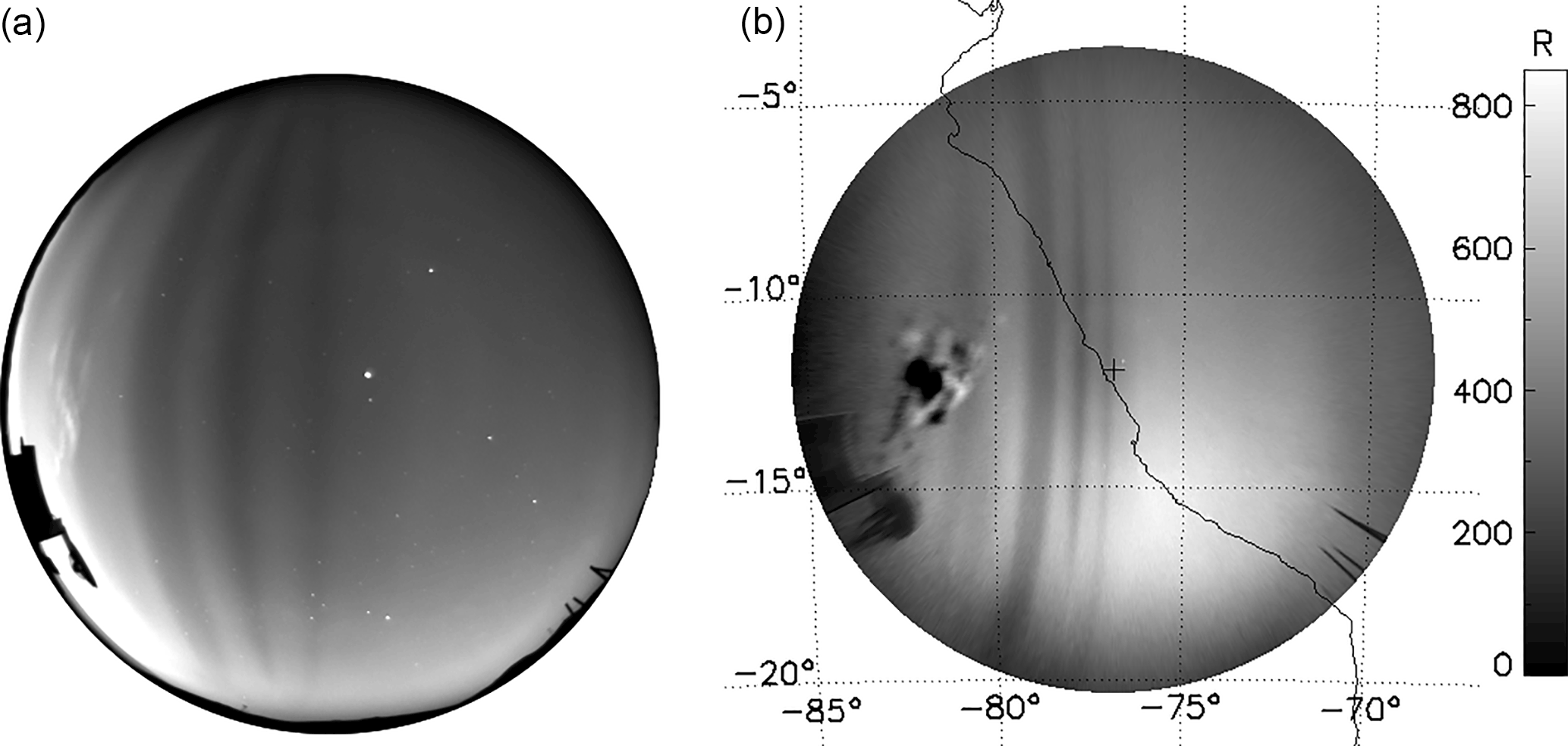
Figure 2(a) A raw image at 05:18 UT on 3 April 2014 from the Jicamarca ASI. The exposure time is 120 s and the image was obtained using a 6300 Å filter. Clouds are visible on the left edge of the image. (b) The unwarped image. The top of the image is north and the left of the image is west. The western coast of South America is seen as a black line and the location of the ASI is marked with a small black cross. The dotted lines are geographic latitudes and longitudes. Latitude and longitude are determined for each pixel, and the image is transferred to a map projection. The grayscale shows the brightness in rayleighs. Clouds low on the horizon are now more prominent in the unwarped image. They also contain dark areas due to background subtraction.
To unwarp the image we assume an emission height of 250 km and use zenith angles between 0 and 80∘ to determine the longitude and latitude of each pixel. A geographical map with longitude and latitude grid lines is overlaid on the image. We subtract the background image from the 6300 Å image, divide by the exposure time, and multiply by a constant factor to determine the emission in rayleighs (Baumgardner et al., 2008). We remove the stars from the images using an algorithm that replaces brighter pixels with the median of the surrounding pixels. The plasma depletions in the raw images are curved and extend from north to south, covering the entire field of view. In the unwarped images the plasma depletions are visible as mostly straight bands that are aligned in the N–S direction.
Collocated with the Jicamarca ASI, an FPI is used to measure neutral winds and temperatures. The FPI uses the Doppler shift and Doppler width of the 6300 Å emission to determine these parameters (Meriwether et al., 2008).
In addition to the optical instruments, we use the radar at Jicamarca in two different modes. We use the ISR mode and a configuration known as the Jicamarca Unattended Long-term Investigations of the Ionosphere and Atmosphere (JULIA). They both operate at 50 MHz. The ISR mode is used to measure ion and electron temperatures, electron densities, and line-of-sight velocities. The JULIA mode detects small-scale irregularities. In this mode the radar detects coherent echoes from density irregularities that are half the wavelength of the radar (3 m), i.e., JULIA detects ESF by measuring the signal-to-noise ratio of the coherent scatter from small-scale plasma density fluctuations.
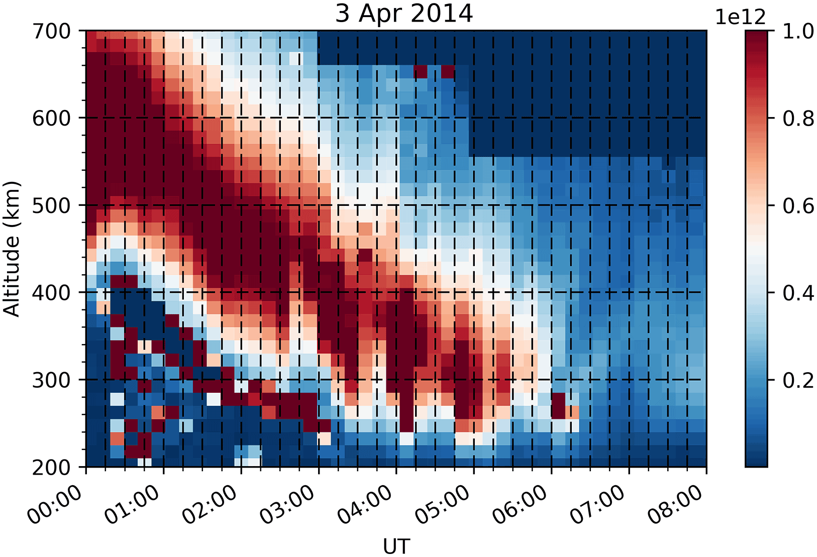
Figure 3A range–time–intensity (RTI) plot from 3 April 2014 showing electron density as a function of altitude and Universal Time. The highest density region that moves down through the night is the F layer. Regions of low density associated with depletions are seen beginning just before 03:00 UT.
On nights when the ISR mode of the Jicamarca main array is running, such as the night presented in Fig. 2, we can use it to measure electron density, ion temperature, and electron temperature at multiple altitudes concurrently. These measurements are used to compare with and add context to the ASI observations. This radar mode uses much more power than the JULIA mode and thus is not run as frequently. Figure 3 shows a range–time–intensity (RTI) plot from the ISR, where intensity depicts electron density, on 3 April 2014, a night when many depletions were observed with the Jicamarca ASI. The F region of the ionosphere is visible as the red region. The peak of the F region is above 500 km at the beginning of the night and then moves down to 300 km. The brightness of an ASI image is mostly determined by the height and density of the F region, which the ISR measures. Similar RTI plots can be made for ion and electron temperatures that are used for analysis of and comparison with ASI images.
We also have concurrent measurements of ESF at Jicamarca with the ASI and the JULIA mode of the main array. Typically, the coherent and incoherent radar modes do not operate at the same time so we only compare with one of each on a given night. On 29 October 2014 both the JULIA mode and the ASI detected features associated with ESF. Figure 4 shows an RTI plot from the JULIA mode. Here, the intensity shows the signal-to-noise ratio of backscatter from 3 m irregularities as they pass over the radar. Figure 4 should not be interpreted as a two-dimensional spatial representation of ESF. These features evolve as they drift past the radar (Hysell and Burcham, 2002). Figure 4 is useful for determining when and where irregularities occur above the radar. From around 01:00 to 02:00 UT there are bottom-type radar echoes and after that bottomside and topside echoes appear. The topside irregularities reach almost 800 km. After about 05:00 UT no strong irregularities are observed.
This combination of instruments at Jicamarca provides a unique opportunity for measuring features associated with ESF. We are able to compare the large-scale features with the small-scale irregularities during concurrent observations with the ASI and JULIA radar mode. When the ISR is running we are able to measure the ionospheric parameters to remove ambiguities in the ASI observations.
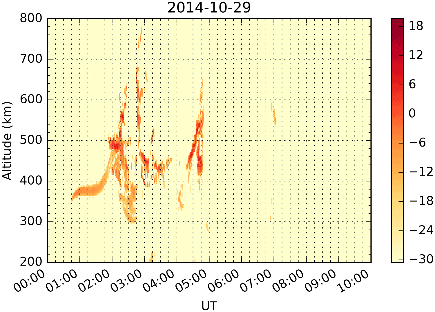
Figure 4A range–time–intensity plot from 29 October 2014 showing signal-to-noise in decibels as a function of altitude and Universal Time. During this night bottom-type, bottomside, and topside ESF irregularities are visible.
In this section we discuss ASI observations of phenomena in the Earth's ionosphere, focusing on ESF. We start by discussing observations at the magnetic equator. At the end of this section we transition to observations related to higher latitudes, though still in the low-latitude region.
3.1 Airglow brightness at the magnetic equator
We initiate the discussion by performing a detailed analysis of airglow brightness at the magnetic equator. The airglow emission is a measure of the number of photons emitted by the upper atmosphere. An absolute calibration of this allows for a more detailed analysis of the images because the brightness can be directly related to the atmospheric parameters. Although operating an ASI at Jicamarca has the advantage of being collocated with many instruments, the magnetic field orientation at the magnetic equator that supports the creation of ESF also complicates ASI observations. The intensity of the airglow emission depends on the plasma density and its altitude distribution. If the peak of electron density occurs at a high altitude, higher than 350 km for most cases, then the airglow emission at 6300 Å is weak. Just after sunset at the magnetic equator there is a large upward E×B drift due to an enhancement in the eastward zonal electric field known as the pre-reversal enhancement (e.g., Fesen et al., 2000). This upward drift raises the F layer early in the night; during this time it is difficult to observe with the ASI due to decreased production of 6300 Å emission. We show in Fig. 5a the measurement of brightness (in rayleighs) at zenith from the ASI throughout the night of 3 April 2014. The values are an average from a 16 × 16 pixel (corresponding to a spatial area of about 70 km × 70 km) box centered at zenith in the unwarped images. The error bars are the standard deviation in this measurement. Additionally, by testing the imagers that we operate we have determined that there is a calibration uncertainty of about 20 %. No data are available between 00:00 and 01:00 UT due to cloudy conditions. Missing data later in the night are also due to clouds.
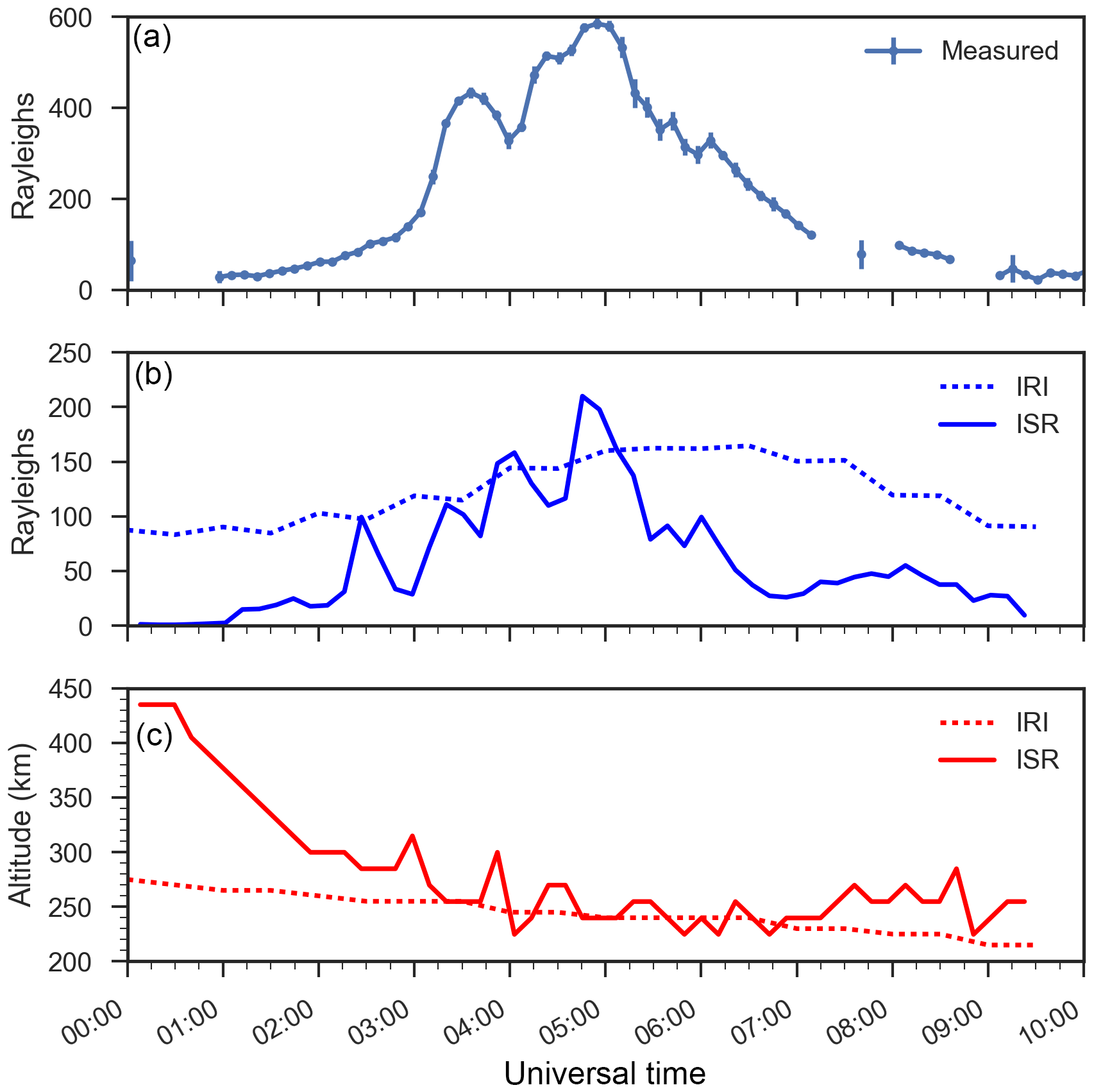
Figure 5(a) 6300 Å emission at zenith on 3 April 2014 as a function of Universal Time. Brightness values are in rayleighs. Episodic decreases in brightness at 04:00 UT and later are due to depletions passing through the field of view. (b) A model output from the BU airglow model showing brightness in rayleighs as a function of Universal Time. The dotted line uses IRI-2012 for values of electron density and plasma temperature, and the solid line uses data measured by the ISR at the Jicamarca Radio Observatory. The vertical axis is a different scale for the top and middle. (c) Altitude of peak emission as a function Universal Time also from the BU airglow model. The solid line uses data measured by the ISR at the Jicamarca Radio Observatory. The dotted line uses IRI for values of electron density and plasma temperature.
From 00:00 to 02:00 UT the brightness is low but then increases to reach a peak around 05:00 UT. After this time the brightness decreases until the end of the night. The shorter timescale decreases in brightness, at 04:00 UT for example, are due to ESF depletions passing through zenith.
An airglow model developed at BU is used to obtain the absolute emission in rayleighs and height of the 6300 Å emission (Semeter et al., 1996). The model uses electron density, electron temperature, ion temperature, O2 density, N2 density, O density, and neutral temperature profiles as inputs. The neutral inputs come from the NRLMSISE-00 atmosphere model (Picone et al., 2002). The ionospheric inputs come from the International Reference Ionosphere (IRI-2012) model (Bilitza, 2015) or from ISR data when available. For the night of 3 April 2014, presented in Fig. 5, the ISR was running so we are able to run the model using radar data. Results from this model are shown in Fig. 5b. The blue solid line is obtained when using ISR data. We also show outputs using IRI-2012 (blue dashed line) to see how they compare. Figure 5c shows peak emission altitudes. The red dotted line indicates model results using inputs from IRI and the red solid line is the result using data from ISR. The ISR electron densities used in the model were shown in Fig. 3.
Early in the night, both model outputs show a trend that is similar to the measured brightness, although the IRI version has a greater emission. During this same time the IRI altitude of emission is lower than the ISR altitude of emission. The IRI model emission stays high later in the night while the measured and ISR version decrease. It is not surprising that the results using IRI-2012 are not as accurate as the ones using ISR because it is an empirical model of climatology.
The overall trend of the modeled airglow using ISR data is very similar to the measured airglow emission, which means that it is mostly the variation in electron density that drives the changes in airglow emission. Additionally, the model using ISR data reproduces certain features such as the local maxima around 05:00 UT and the large depletion at 04:00 UT. There are some increases in brightness from the model result that are not seen in the measured airglow, such as the peak at 02:30 UT. From Fig. 3 we see that this occurs in a region where there is a sharp gradient in electron density. The lower-density region that is causing this gradient is a plasma depletion. Sharp gradients produced by ESF depletions can impact the ISR measurements and are an extra source of error during these times.
We use ISR density measurements to determine what causes the airglow emission to vary. Early in the night the F layer is very high in altitude with the peak density being higher than 500 km (Fig. 3), which causes weak 6300 Å emission. As the night progresses the layer moves down and the brightness increases. The peak emission during the night occurs when the F layer has moved down to low altitude but still has a similar peak density. After this the electron density decreases and the emission in both the images and the models decreases. Thus, it is clear that the electron density is the major driver of airglow variation.
The measured airglow is much greater than the modeled airglow, even when accounting for up to 20 % error in calibration. We use measured electron density from the ISR as an input so it is unlikely that electron density is the reason for the discrepancy. Since the BU airglow model also uses neutral density, it relies on the accuracy of NRLMSISE-00. One way to match the model to the observations is to increase O2 by a factor of 3. While the neutral density may play some role in the discrepancy, we do not believe it is the main factor. We believe that scattered light from the surrounding area, Lima, created the excess airglow. We examined other cases and found that when fog and low clouds block the light from Lima, the measured results are closer to the modeled results. We did this same analysis at El Leoncito, where there is minimal contamination from city lights, and found that the model results were typically within the calibration error of 20 % of the measured values. Although the measured airglow at Jicamarca may not be accurate in its absolute intensity, we identified depletions and measured their movement and morphology. The airglow model allows us to better determine the altitude of emission when measuring these characteristics.
3.2 Depletion patterns and morphology
ASI images that contain multiple airglow depletions associated with ESF can be analyzed to characterize their spatial morphology. We measure the distance between depletions and between groups of depletions to investigate the presence of LSWSs.
ESF depletions are visible at Jicamarca during most of the clear nights. Out of the 517 nights, 387 nights were too cloudy to make a conclusion about the presence of ESF. Out of the remaining 130 clear nights, depletions were observed in 120. In only 10 nights were ESF structures not observed at Jicamarca. The identification of airglow depletions associated with ESF is relatively straightforward as they are bands of lower intensity that extend from north to south. It is possible that undulations in the bottomside could create similar airglow structuring, but in general we can distinguish between ESF related structures and other perturbations. Depletions associated with ESF at Jicamarca tend to travel eastward and have a well-defined band structure that curves to the west away from zenith. We do not expect other undulations to move in the same way and have the same extent and shape in the field of view. Precursors to post-midnight ESF as described in Rodrigues et al. (2018) show airglow structures that are not associated with ESF and are likely due to LSWS. Equatorial spread F structures tend to move with regular motion eastward and the precursors Rodrigues et al. (2018) had very little motion, often staying in the same location for multiple images. In the analysis here the structures are observed over multiple images and we wait until the structures are fully formed to measure their properties, so we do not think that ESF precursors impact our analysis. From our observations, depletions occur just after sunset and in some cases just before sunrise. In almost all cases the depletions tend to come in groups. We measured the smaller distance between the depletions within the groups and measured the distance between the groups. The distance between depletions was taken to be the distance from the center of one depletion to another. To determine the distance between groups, we locate the center of a group and measure the distance to the next group. The center of the group is the midpoint between the outermost depletions. An example of the grouping is shown in Fig. 6. In this example, there are two groups of depletions with a group-to-group separation of ∼ 320 km. The distance between the depletions (marked by blue arrows) in this example ranges from 50 to 110 km. Analysis of all the nights in our sample showed that there were typically close groups of two to four depletions separated by ∼ 50–100 km. The group-to-group separation was typically between 400 and 500 km. Consecutive depletions that were closer than 300 km were considered to be in the same group. We found no seasonal variation in the separation distance, number of depletions in the groups, or grouping distance.
Previous studies using ASI that measured the distance between depletions, discussed in Sect. 1, did not measure or discuss any group distances. They found that the structures were typically separated by 100–300 km. Therefore, our analysis of the Jicamarca ASI images is the first of its kind. Another difference between these results and the previous studies is that our observations are during solar maximum (F10.7 ≈ 100–150 sfu), while the other studies were done during two different solar minimums. The observations in Makela et al. (2010) were taken from 2006 to 2009 (F10.7 ≈ 70 sfu), and the Chapagain et al. (2011) observations were done in 1995 (F10.7 ≈ 80 sfu).

Figure 6An example from 3 April 2014 of how depletion separation is measured. Panel (a) is an unwarped ASI image with two groups of depletions visible. Panel (b) shows brightness at a line of constant latitude that passes through zenith. The red dotted lines show the four lines of longitude from the image and the center of the image where the ASI is located. The blue arrows show the locations of the depletions. The distance between the depletion groups is shown in red at the top of the image. The center of these groups are marked by the edges of the red line.
The separation of the groupings in our observations indicates that an LSWS on the order of 400–500 km may be modulating the formation of ESF depletions, causing them to appear in groups. This is consistent with the study from Tsunoda and White (1981), where it was noted that ESF plumes were forming at the crest of LSWS where the F layer had moved up. The rising of the F layer around sunset, due to the pre-reversal enhancement, is understood to play an important role in the formation of ESF. It has also been shown that even a small rise later in the night can increase the likelihood of ESF (Ajith et al., 2016). An LSWS could provide the small rise, creating the groups of depletions.
Occasionally separations much larger than 500 km (e.g., 1000 km or more) were observed. For these cases it seems more likely that something other than an LSWS is causing this modulation. It is possible that other dynamics are causing the F layer to rise or there is some other variation affecting the growth rate. It is interesting to note that we only observe bottomside structures in this study and for most cases we are not able to determine if they are forming topside plumes. Tsunoda and White (1981) looked at the modulation of plumes that formed from bottomside ESF. Our results indicate that these waves not only modulate the creation of topside plumes but also modulate the bottomside structures that do not form plumes.
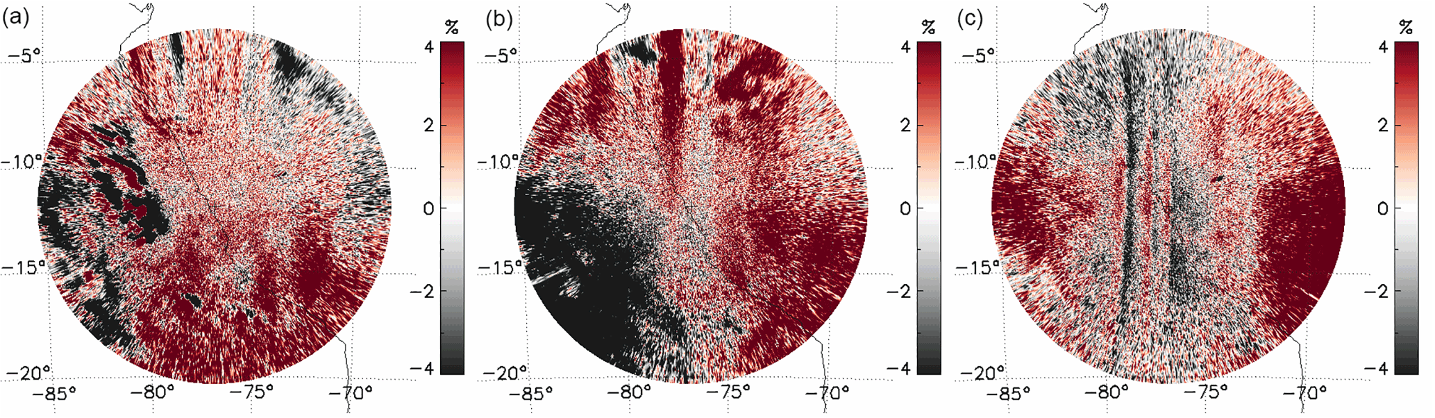
Figure 7Three unwarped difference images from 29 October 2014. These images show the difference between two consecutive images by subtracting the earlier image from the later image. These images are then scaled to their average value in order to show increase and decrease as a percent. Red is positive, black is negative, white shows no difference, and the color scale shows the difference values in percent. This technique brings out details that may not be as clear in images like Fig. 2. Airglow depletions in these images are visible as alternating red and black regions. The depletions move between images so subtracting the earlier image from the later image means that both positive and negative values can indicate depletions. Positive values indicate the western edge of depletions in the earlier image and negative values indicate the eastern edge of depletions in the later image. Values close to zero between red and black regions are where the depletions overlap. Coordinates show geographic latitude and longitude. The plus sign in (b) is the location of the ASI. The black line shows the western coast of Peru. (a) Unwarped image 03:36 UT (LT = UT − 5). Clouds are responsible for the black patches to the west of −80∘. Depletions are visible at the northern edge of the image. (b) Unwarped image at 04:31 UT. The red band around −77∘ and adjacent darker regions show the presence of a depletion extending from the north down past zenith. (c) Unwarped image at 09:08 UT. Three depletions are visible between −80 and −75∘ longitude.
3.3 Coherent scatter radar and ASI comparison
We use the JULIA mode of the radar to compare the small-scale irregularities with large-scale depletions. Figure 7 shows three ASI difference images from the same night as Fig. 4. The difference images are created using two consecutive images and subtracting the earlier image from the later image. This makes faint features easier to detect. The difference image in Fig. 7a is from 03:36 UT, about 3 h after sunset (LT = UT − 5), and faint depletions are visible only at the top of the image due to very weak emission. Figure 7b shows a difference image at 04:31 UT. A depletion is visible through much of the image as the overall 6300 Å emission increases. Figure 7c shows an image from 09:08 UT; here the emission is greater and three depletions extending from north to south are visible.
For this night we can directly observe that there are concurrent airglow depletions and small-scale irregularities, but recently Rodrigues et al. (2018) showed that airglow signatures can occur before post-midnight irregularities. In the ASI images from this night, depletions in the entire field of view are only visible after 04:00 UT yet there are large plumes of irregularities visible in the RTI plots earlier. Although low emission early in the night leads to difficult observing conditions at zenith in the ASI images, sometimes ESF depletions can be seen near the edge of the images away from the magnetic equator. The rising of the F layer is most prominent at the center of the image, which is at the magnetic equator. At the edges of the image, the layer might not move up much. Additionally, the fountain effect that creates the crests of equatorial ionization anomaly (EIA) may be redistributing some of the plasma from the magnetic equator to the edge of the images. Both of these factors can lead to features being visible on the edge of the images early in the night when no depletions are visible at the center. On this night, edge features are visible as early as 03:36 UT, as seen in Fig. 7, but the RTI shows irregularities starting prior to 01:00 UT. The airglow emission is too faint to observe the large-scale structures associated with the irregularities visible early in the night.
The rising of the F layer that decreases airglow plays an important role in the generation of ESF. The formation of ESF is due to the generalized Rayleigh–Taylor instability and the instability growth rate is shown in Sultan (1996). As the F layer rises the growth rate of the generalized Rayleigh–Taylor instability increases, mainly due to three terms in the growth rate equation. First, an upward plasma drift increases the growth rate. The other two terms are related to a decrease in background neutral density at higher altitudes. This lowers both the collision frequency and the recombination rate. A larger growth rate means that bottomside ESF is more likely to form. As a result, most ESF at Jicamarca occurs during post-sunset hours. Although it is challenging to observe depletions associated with ESF early in the night with the ASI, irregularities associated with ESF are easily observed with coherent scatter radar using the JULIA mode. Using this mode the irregularities associated with ESF are observed before they are visible in the ASI.
3.4 Higher-latitude ESF effects
ASI depletions observed at low latitudes can be related to ESF structures observed at the magnetic equator. In addition to using the Jicamarca ASI to observe bottomside depletions, we use the El Leoncito and Villa de Leyva ASIs to observe topside depletions. On 29 October 2014, the night with data shown in Figs. 4 and 7, the El Leoncito and Villa de Leyva ASIs also detected airglow depletions. Images from El Leoncito on this night are shown in Fig. 8. At 03:31 UT there is a large depletion at around −75∘ longitude that extends from the top to the middle of the image. Due to its higher latitude, these depletions are topside plumes that have apex altitudes above 1100 km. This same depletion is located in the center of the images taken around 04:30 UT. Figure 9 shows images from the Villa de Leyva, Jicamarca, and El Leoncito ASIs from that same night at 04:52 UT. At Villa de Leyva there were clouds during most of the night, some of which are present in this image, but we are still able to determine the presence of airglow depletions. Two depletions are visible between −75 and −70∘ longitude, extending from the bottom of the image to 700 and 900 km magnetic apex altitude. They are marked by red and blue arrows. At the same time these structures have conjugate depletions at El Leoncito. At Villa de Leyva the depletions extend from the southern edge of the image to the north while those at El Leoncito extend from the northern edge of the image to the south because they are flux-tube aligned with vertical structures at the magnetic equator. There are also clouds in the field of view of the El Leoncito image (creating the dark horizontal bands around 700 km magnetic apex) but a depletion is visible at about −68∘ longitude, marked by a red arrow, which is the conjugate depletion of the one at Villa de Leyva around −70∘ longitude, also marked by a red arrow. Another depletion is just barely visible at El Leoncito around −71∘, marked by a blue arrow, which is conjugate to the depletion around −74∘, marked by a blue arrow. Low emission at Jicamarca makes it difficult to observe but there is a depletion near zenith, marked by a green arrow.
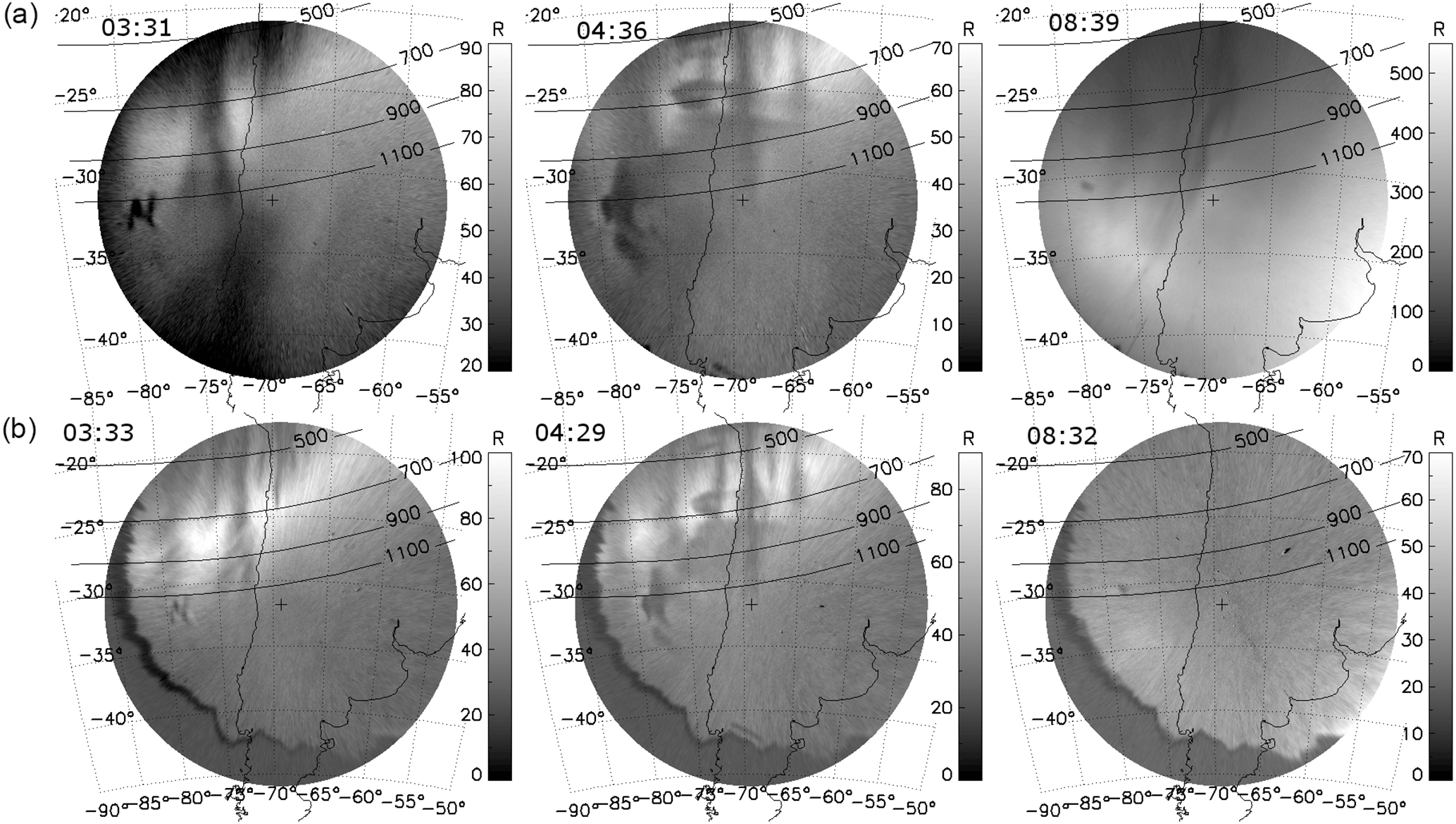
Figure 8Unwarped images from the El Leoncito ASI on 29 October 2014. Row (a) shows 6300 Å images and row (b) shows corresponding 7774 Å images. Dotted lines represent geographic latitude and longitude. The plus sign in the middle is the location of the ASI. The map shows the coasts of South America. Lines of constant magnetic apex altitude are shown from 500 to 1100 km. Depletions are visible extending from the north to zenith. The bright band visible in the north in the earlier images is the crest of the equatorial ionization anomaly. At 08:39 UT the 6300 Å emission is much greater due to the presence of a BW.

Figure 9Three unwarped images from the Villa de Leyva (a), Jicamarca (b), and El Leoncito (c) ASIs on 29 October 2014 at 04:52 UT. Dotted lines represent geographic latitude and longitude. The plus sign in the middle of each image is the location of the ASI. The map shows the coasts of South America. Lines of constant magnetic apex altitude are shown from 500 to 1100 km. Clouds cover a lot of the Villa de Leyva image but two depletions are visible between −75 and −70∘ longitude, extending to 700 and 1100 km magnetic apex altitude. One is marked by a blue arrow and one with a red arrow. These depletions are also visible in the El Leoncito image but clouds are also in the field of view. The blue arrow at El Leoncito marks the depletion associated with the blue arrow at Villa de Leyva. The red arrow at El Leoncito marks the depletion associated with the red arrow at Villa de Leyva. At Jicamarca there is one depletion that is barely visible near zenith, marked with a green arrow.
Although early in the night at Jicamarca we only see depletions at the edge of the ASI images, we can see a large-scale depletion at 03:33 UT with the El Leoncito ASI (Fig. 8). This depletion is about 3∘ to the east of the Jicamarca radar. We determine that this depletion is associated with the largest irregularity plume observed with the JULIA mode of the radar (Fig. 4). This irregularity plume occurs just before 03:00 UT and irregularities are visible up to 800 km in altitude. The depletion has an apex altitude greater than 1100 km, which is beyond the maximum altitude of the JULIA mode, but from 700 to 800 km only relatively weak echoes are observed. At 04:30 UT depletions just start to appear in the field of view of the El Leoncito ASI (Fig. 8). At 04:52 UT there are depletions visible at Villa de Leyva and El Leoncito (Fig. 9) when the airglow is still weak at Jicamarca and depletions are still only faintly visible. These depletions are associated with a plume of irregularities visible just before 05:00 UT (Fig. 4). In Fig. 9 the plumes extend to 1100 km in apex altitude but irregularities are only observed up to 650 km with the JULIA mode. Similar to the comparison at an earlier time, strong irregularities are not observed throughout the entire depletion.
The El Leoncito ASI also provides information about the EIA that redistributes low-latitude plasma, decreasing the 6300 Å emission at the magnetic equator. In Fig. 8 the 7774 Å images show the location of the southern crest of the anomaly early in the night. The crest of the anomaly is identified as the bright band at the top of the images around 25∘ S at 03:33 and 04:29 UT. From 03:33 to 04:29 the crest moves toward the Equator and the emission at 7774 and 6300 Å decreases. This indicates that the plasma is moving back to the magnetic equator. The strong EIA crest early explains why the emission is weak at the magnetic equator, and why, as it diminishes, the emission at the magnetic equator increases. At the end of the night, the EIA crest is no longer visible at El Leoncito because the plasma that formed the crest has moved back to the magnetic equator.
Later in the night we can detect depletions with the Jicamarca and El Leoncito ASIs that are not observed with the JULIA radar. These are “fossilized” depletions that were not formed over the radar and enter the field of view fully formed so the small-scale irregularities have dissipated. Figure 7 shows depletions at 09:08 UT on 29 October 2014 observed with the Jicamarca ASI and Fig. 8 shows depletions at 08:39 UT on the same night observed with the El Leoncito ASI. Figure 4 shows that no small-scale irregularities are observed after 08:00 UT. In addition to comparisons when features are visible with both instruments, these two instruments complement each other by providing information when one system does not detect ESF features.
In RTI plots there is often a disruption in bottomside irregularities when topside plumes are visible (e.g., Hysell and Burcham, 2002). In Fig. 4 this can be seen at 03:00 UT as the bottom-side irregularities are no longer visible and a large plume has risen to the topside. To complement this we compare observations of bottomside airglow depletions at Jicamarca with topside airglow depletions at El Leoncito. Figure 10 shows concurrent images from 3 April 2014, where bottomside depletions are visible at Jicamarca and topside depletions are visible at El Leoncito. We see that although there is a group of depletions visible at Jicamarca, we only observe one topside plume. We are unable to determine which bottomside depletion becomes a topside plume or if the bottomside features merged to form one plume since the topside plume is as wide as the group of depletions. Equatorial spread F plumes are not expected to have the same width at all altitudes and can be wider at higher altitudes (e.g., Retterer, 2010). We have looked at other cases and have found that we only observe one topside plume associated with a group of bottomside depletions. Another possibility is that the bottomside depletions evolved into plumes that merged (e.g., Huang et al., 2012). We were not able to find any significant differences between bottomside depletions (e.g., relative brightness of the depletion compared to the background or its width) that form plumes and those that do not.
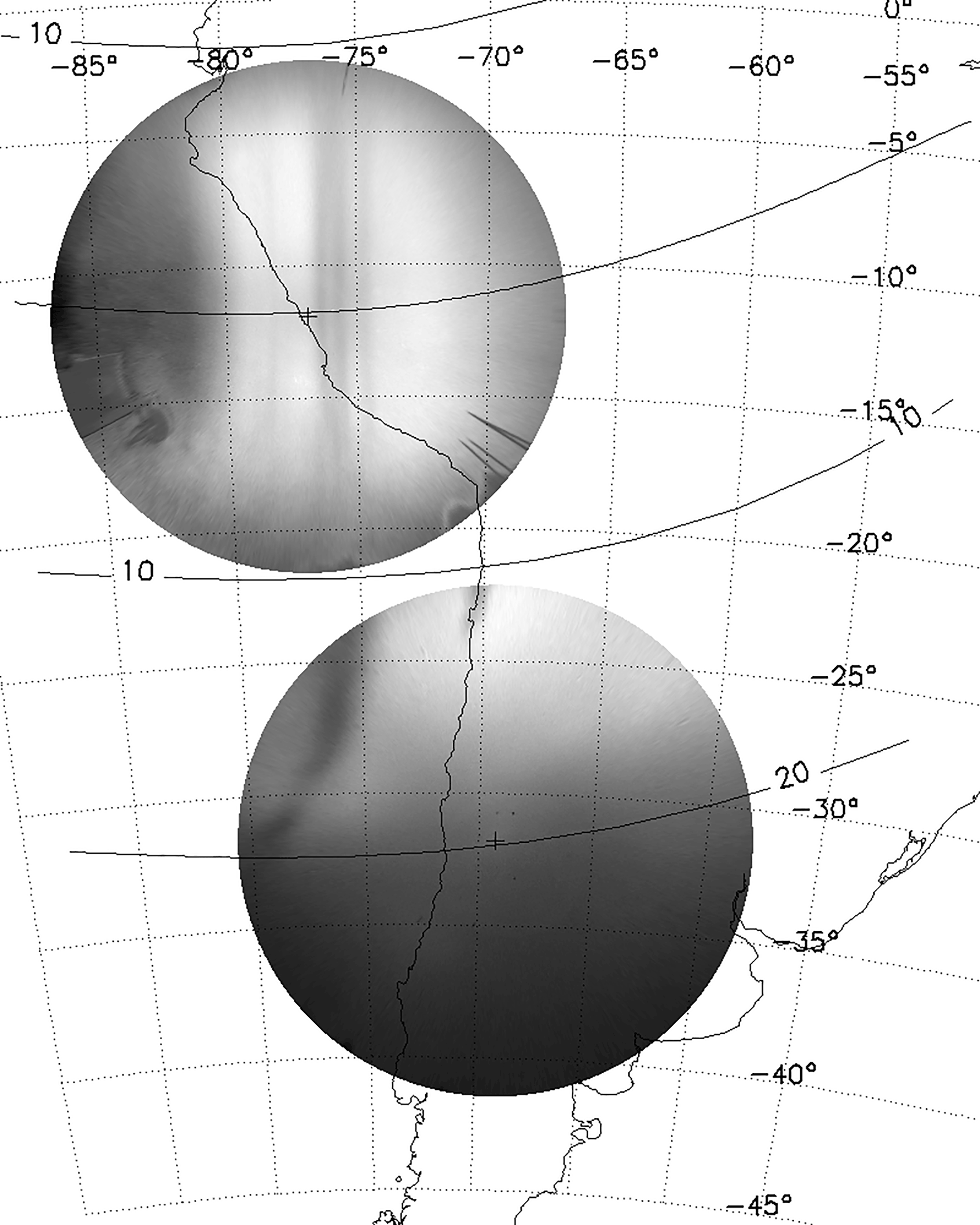
Figure 10Unwarped images from Jicamarca and El Leoncito on 3 April 2014. The Jicamarca image is at 04:15 UT and the El Leoncito image is at 04:18 UT. At Jicamarca bottomside depletions are visible and at El Leoncito topside plumes are visible. The magnetic equator is shown passing through the Jicamarca ASI field of view and lines of magnetic latitude at 10 and 20∘ are shown as well. The two images do not have the same color scale in order to make the features more clearly visible.
In this section we discuss phenomena related to the neutral atmosphere that we can investigate using ASIs. We discuss neutral winds in the thermosphere and the MTM.
4.1 Airglow and thermospheric processes
An FPI at Jicamarca is used to measure neutral winds and temperatures. Zonal neutral winds are related to the motion of plasma through the F region dynamo. The neutral temperatures measured by the FPI are also used to detect and measure the MTM.
The zonal motion of the depletions across the field of view of the ASI can be used to investigate the zonal plasma drifts at the magnetic equator. At night the zonal plasma drifts are driven mostly by the neutral winds through the F region dynamo (Rishbeth, 1971). We measure the neutral winds with an FPI and the plasma drifts inferred from the depletion motion to make a comparison. There are various ways to determine plasma motion from ASI images (Chapagain et al., 2013; Makela and Kelley, 2003), but here we track a depletion through a series of images and from that we determine a zonal drift. We present a case study from 3 April 2014, where we have about 3 h of concurrent measurements from the FPI and ASI at the Jicamarca Radio Observatory. We determine the location of the minimum of the depletion and track it as it moves through the field of view. Figure 11 shows the comparison between the zonal plasma drifts derived from the ASI and the zonal winds measured by the FPI.
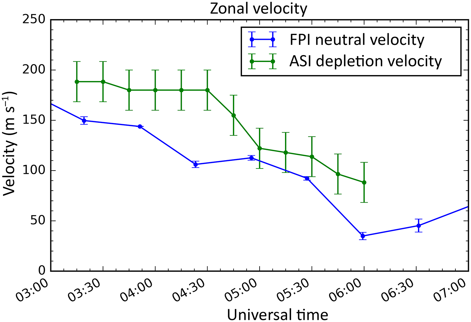
Figure 11Zonal neutral winds (blue) and zonal plasma drifts (green) on 3 April 2014 at Jicamarca. Zonal wind speeds are determined by an FPI and plasma drifts are determined from depletion velocities.
The plasma drifts show a similar trend as the FPI neutral winds with an overall reduction in magnitude after 03:00 UT. The velocity of the depletions is higher than the velocity of the neutrals. We consider potential errors in the determination of the depletion velocities that could affect the absolute magnitude of the drifts. Images were unwarped assuming an altitude of 250 km. A 50 km difference would modify the zonal drift calculation by ∼ 15 %. From Fig. 5 the calculated height is greater than 250 km from 03:00 to 04:00 UT, so the drifts would be larger than the ones shown in Fig. 11. At 04:00 UT the modeled altitude of emission is most likely lower than reality because of a depletion that causes the electron density in the ISR data to be lower than the background. After 04:00 UT the height is closer to 250 km, but is slightly lower. Thus, we may be underestimating the zonal plasma velocity earlier in the night and overestimating it later in the night. In addition to the error from the uncertainty in altitude there is also the associated error from determining the center of the depletion and from the fact that depletions tend to evolve as they pass through the field of view. These errors have been accounted for in the error bars in Fig. 11.
Chapagain et al. (2013) did a comprehensive study in Brazil comparing depletion velocities to neutral winds from FPIs. They found that during most nights the velocities matched, but there were some cases where they did not. During some nights the depletion velocities were slower than the neutral winds and during other nights the depletions velocities were faster. If the plasma depletions match the neutral winds, then the F region dynamo is fully active.
In order to understand the results from Fig. 11 we refer to Eq. (1) from Martinis et al. (2003) that shows the different quantities that determine the zonal drift velocity.
Vϕ and VL are the zonal and vertical plasma drifts, is the Pedersen conductivity-weighted neutral zonal wind, JL is the integrated vertical current density, and ΣP and ΣH are the field-line-integrated Pedersen and Hall conductivities. The plasma drift, Vϕ, is typically equal to , meaning that the F region dynamo drives the plasma motion. creates a vertical electric field and contributes to plasma motion through an E×B drift. The other terms make minor adjustments to Vϕ. A fully operating F region dynamo means that the plasma drifts are equal to the first term on the right hand side. If the depletions move slower than the neutral velocity then upward vertical plasma drifts or vertical current density may cause this difference. If the depletion velocity is faster than the neutral winds then one of the terms on the right side of Eq. (1) may be responsible for this. The depletion velocity measurements made by Chapagain et al. (2013) were not at the magnetic equator so the depletion velocities were associated with higher altitudes than where the FPI measurements are made, which were not collocated and were closer to the magnetic equator. Neutral winds may be greater at these higher altitudes and could explain why they measured faster plasma drifts. The ASI and FPI that we use are collocated so there is no difference in altitude in our measurements. The vertical plasma drift term on the right side of Eq. (1) can increase the zonal drift velocity if there is a downward plasma motion. The ISR measurements in Fig. 3 show that there is a downward motion of the plasma during the times when zonal plasma drifts are faster than the neutral winds. This is a likely explanation for the difference in velocities earlier in the night.
Another prevalent low-latitude neutral process that we observe is the MTM, an increase in temperature (neutral, ion, and electron) near local midnight. Figure 12 shows neutral and ion temperature at an altitude of 250 km on 4 April 2014. Although we only present one altitude from the ISR measurements, the MTM occurs at multiple altitudes (Martinis et al., 2013; Hickey et al., 2014). The temperature increase begins just before 05:00 UT and the peak of the temperature increase is just after 06:00 UT (LT = UT − 5). The local maximum in temperature that is measured by both instruments is the MTM. There is very good agreement between the two measurements meaning that the ion temperature is equal to the neutral temperature, as previously shown by Hickey et al. (2014). The magnitude of the ion and neutral temperature increases are between 50 and 100 K. These observations are compared with higher-latitude ASI observations in the next section to constrain the morphology of the MTM.
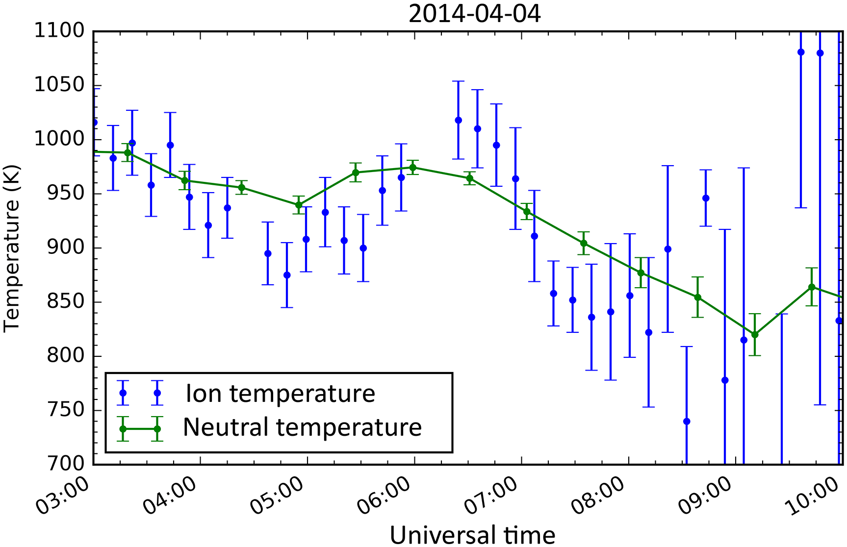
Figure 12An MTM observed on 4 April 2014. Blue dots show the ion temperatures as measured by the ISR. Green points are the neutral temperatures measured by the FPI. The peak of the MTM occurs between 06:00 and 06:30 UT (01:00 and 01:30 LT).
4.2 Higher-latitude MTM effects
At mid-latitudes, the effects of the MTM can be observed by an ASI as an increase in brightness that travels poleward. There was no BW associated with the MTM in Fig. 12 in the ASI images at Jicamarca. The magnetic field lines are mostly horizontal throughout the entire field of view of the ASI so the winds associated with the MTM would not be able to move the plasma downward enough to increase the airglow emission.
On 4 April 2014, the same night as in Fig. 12, we observed a BW with the ASI at El Leoncito. Figure 13 shows the brightness calculated from a 16×16 pixel box at zenith. In contrast to Fig. 5, which shows very weak airglow at Jicamarca early in the night, at El Leoncito the emission is greater early in the night and decreases throughout the night. This is partially due to the fact that the rising of the F layer early in the night at Jicamarca, the source of the equatorial fountain effect, moves the plasma toward El Leoncito, increasing the airglow emission. Additionally, since the F layer does not rise in altitude at El Leoncito, the altitude of the plasma creates greater emission. As the night goes on, recombination leads to a decrease in the ionosphere, thus decreasing the emission at El Leoncito. At around 06:30 UT the brightness begins to increase until it reaches a peak just after 08:00 UT. This increase in brightness is what we define as a BW and associate with the MTM. The BW has an apparent propagation from the northeast to the southwest in the ASI images. This is evident in the video clip shown in the Supplement.
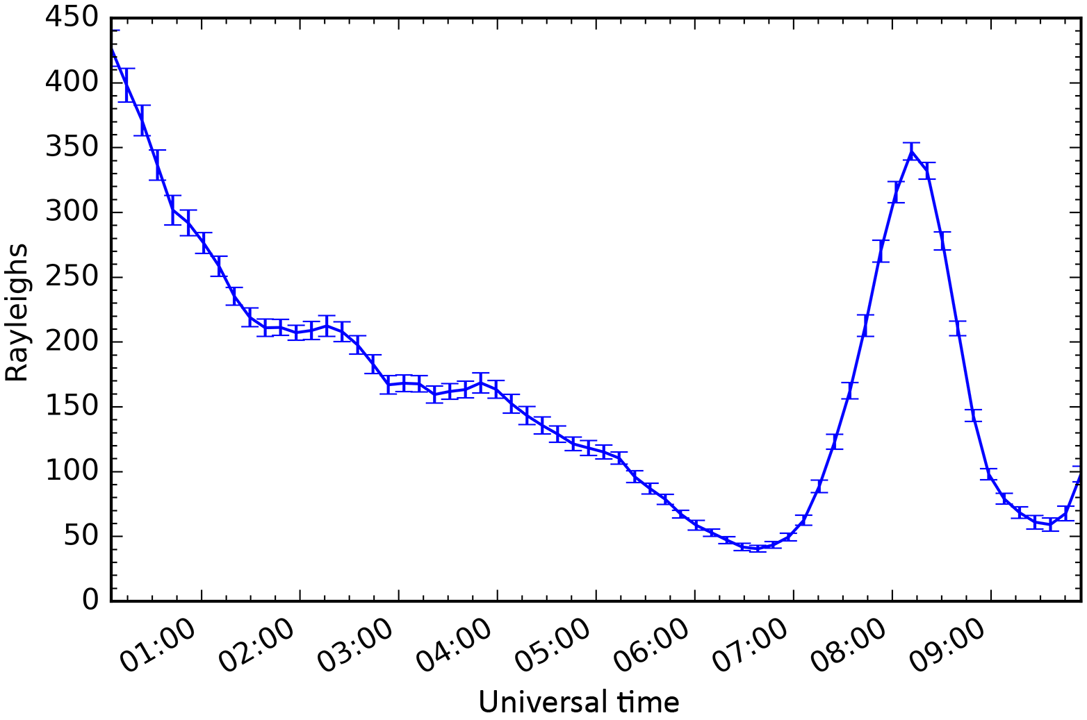
Figure 13Measurement of brightness in rayleighs measured at zenith with the El Leoncito ASI throughout the night on 4 April 2014. Earlier in the night, in contrast to Jicamarca ASI observations, there is the typical decrease in brightness as the ionosphere decays. The increase in brightness later in the night, with a peak at about 08:00 UT, is a brightness wave.
If we assume that the MTM propagates from Jicamarca to El Leoncito, then we can determine the propagation speed. The time delay between the peak of the MTM and the peak of the brightness wave is approximately 2 h, resulting in a speed of about 330 m s−1. This is consistent with the result of a phase velocity of the BW of 200–400 m s−1 from Colerico et al. (2006), but the Jicamarca ASI is located almost 8∘ to the west of El Leoncito, so if the source of the brightness wave was the MTM at Jicamarca, it would not propagate from the northeast to the southwest as is observed. The MTM occurs over a wide range of longitudes (Herrero and Spencer, 1982) and no dependence on longitude has been observed (Spencer et al., 1979); i.e., the MTM occurs near local midnight at all longitudes and thus follows the apparent motion of the Sun (Meriwether et al., 2013; Colerico et al., 1996). From this we expect that at an earlier UT an MTM should occur to the east of Jicamarca. We use the velocity of the brightness wave to determine where the source MTM should be located. The apparent meridional velocity of the brightness waves is 280 m s−1. This is calculated by using the distance that the peak of brightness wave travels from the northern edge of the image to the southern edge of the image and the time it takes for it to travel that distance. At this speed it would take about 2 h to travel from the latitude of Jicamarca (11.95∘ S) to El Leoncito (31.8∘ S) along a constant longitude. The Earth is rotating beneath the MTM so during this time the MTM will be traveling to the west with the speed of the Earth's rotation. With this speed, we find that it would have originated from 38.1∘ W at about 06:00 UT. This is the same time that the MTM is observed at Jicamarca. Given that the MTM follows the apparent motion of the Sun, at approximately the anti-solar point, we do not expect that it should occur at the same UT at two locations separated by 38.8∘ of longitude. The timing of the MTM at Jicamarca leads us to expect an MTM at around 03:40 UT at 38.1∘ W, over 2 h earlier than is expected from the brightness wave observations. Our observations are not consistent with an MTM propagating south from a lower latitude.
We present another explanation for the time delay between the observation of the MTM at Jicamarca and the BW occurrence at El Leoncito, based on global model results of the MTM. Akmaev et al. (2009) used a whole atmosphere model (WAM) to reproduce the MTM that shows an apparent poleward motion due to its morphology. The simulated MTM occurs over a range of latitudes and longitudes such that it makes a sideways “V” shape in longitude–latitude space, consistent with results from Herrero and Spencer (1982). The vertex of the V is located close to the Equator and is oriented so that the two end points of the V are to the east. The whole structure migrates westward following the apparent motion of the Sun. As a result the MTM occurs earliest at the vertex of the V, near the Equator, and occurs later at higher latitudes. WAM outputs are consistent with our result that the MTM occurs first at Jicamarca and that the BW at El Leoncito appears to propagate to the southwest.
In this paper we have shown results from an ASI installed at Jicamarca and collocated instruments. Two ASIs at higher latitudes were also used. Using a 6300 Å filter we are able to observe plasma depletions associated with ESF and a brightness wave associated with the MTM. We investigated several aspects of thermosphere–ionosphere dynamics near the magnetic equator and at low latitudes. We have summarized our results in the following points:
-
We compared small-scale coherent radar echoes with large-scale depletions, showing that early in the night when the airglow emission is weak only the radar is able to detect irregularities with 3 m scale sizes. The El Leoncito ASI is at a site with stronger airglow in this period and is able to detect depletions associated with these irregularities. Groups of depletions tend to form only one topside plume and there is no difference between bottomside depletions that form topside plumes and those that do not. Late in the night at Jicamarca we observe “fossilized” depletions without associated radar echoes, meaning that the smaller-scale structures have already dissipated.
-
Using radar data and NRLMSISE-00, the Boston University airglow code reproduces accurately the trend in the observations, although the peak modeled values are a factor of 2–3 smaller. This inconsistency could be due to contamination from nearby city lights.
-
Airglow depletions occur in groups separated by 400–500 km. Within the groups the separation tended to be 50–100 km. This indicates that an LSWS may be modulating bottomside depletions.
-
We presented a case study comparing the zonal speed of neutral winds and zonal plasma drift obtained from collocated FPI and ASI, respectively. Early in the night the depletions move faster than the neutral winds, a result attributed to downward drifts that modify a fully working F region dynamo.
-
We presented a case study where the MTM was observed at Jicamarca and a BW was observed at El Leoncito. The timing of these two events supports the idea that the MTM has sideways V structure in latitude–longitude space and that the whole structure moves westward with the apparent motion of the Sun.
Preview images from the Boston University all-sky imagers can be found at http://buimaging.com. For access to the raw data use the contact information from the website or contact the author. All the other data are available through the Madrigal CEDAR Database at http://madrigal3.haystack.mit.edu/. JULIA measurements, other Jicamarca data, and contact information can be found at http://jro.igp.gob.pe. Last access: 16 March 2018.
The supplement related to this article is available online at: https://doi.org/10.5194/angeo-36-473-2018-supplement.
The authors declare that they have no conflict of interest.
This work was supported by NSF grant AGS-1123222, NSF grant CEDAR
AGS-1552301,
and ONR grant N00014-13-1-0323. JULIA measurements used in this study were
made available by the Jicamarca Radio Observatory, a facility of the
Instituto Geofisico del Peru operated with support from the NSF AGS-1433968
through Cornell University.
The topical
editor, Ana G. Elias, thanks Inez Batista and one anonymous referee for help
in evaluating this paper.
Ajith, K. K., Tulasi Ram, S., Yamamoto, M., Otsuka, Y., and Niranjan, K.: On the fresh development of equatorial plasma bubbles around the midnight hours of June solstice, J. Geophys. Res.-Space, 121, 9051–9062, https://doi.org/10.1002/2016JA023024, 2016. a
Akmaev, R. a., Wu, F., Fuller-Rowell, T. J., and Wang, H.: Midnight temperature maximum (MTM) in Whole Atmosphere Model (WAM) simulations, Geophys. Res. Lett., 36, L07108, https://doi.org/10.1029/2009GL037759, 2009. a, b
Akmaev, R. A., Wu, F., Fuller-Rowell, T. J., Wang, H., and Iredell, M. D.: Midnight density and temperature maxima, and thermospheric dynamics in Whole Atmosphere Model simulations, J. Geophys. Res., 115, A08326, https://doi.org/10.1029/2010JA015651, 2010. a
Bamgboye, D. K. and McClure, J. P.: Seasonal variation in the occurrence time of the equatorial midnight temperature bulge, Geophys. Res. Lett., 9, 457–460, https://doi.org/10.1029/GL009i004p00457, 1982. a
Baumgardner, J., Wroten, J., Semeter, J., Kozyra, J., Buonsanto, M., Erickson, P., and Mendillo, M.: A very bright SAR arc: implications for extreme magnetosphere-ionosphere coupling, Ann. Geophys., 25, 2593–2608, https://doi.org/10.5194/angeo-25-2593-2007, 2007. a
Bilitza, D.: The International Reference Ionosphere – Status 2013, Adv. Space Res., 55, 1914–1927, https://doi.org/10.1016/j.asr.2014.07.032, 2015. a
Chapagain, N. P., Taylor, M. J., and Eccles, J. V.: Airglow observations and modeling of F region depletion zonal velocities over Christmas Island, J. Geophys. Res.-Space, 116, A02301, https://doi.org/10.1029/2010JA015958, 2011. a, b
Chapagain, N. P., Fisher, D. J., Meriwether, J. W., Chau, J. L., and Makela, J. J.: Comparison of zonal neutral winds with equatorial plasma bubble and plasma drift velocities, J. Geophys. Res.-Space, 118, 1802–1812, https://doi.org/10.1002/jgra.50238, 2013. a, b, c
Colerico, M., Mendillo, M., Nottingham, D., Baumgardner, J., Meriwether, J., Mirick, J., Reinisch, B. W., Scali, J. L., Fesen, C. G., and Biondi, M. A.: Coordinated measurements of F region dynamics related to the thermospheric midnight temperature maximum, J. Geophys. Res.-Space, 101, 26783–26793, https://doi.org/10.1029/96JA02337, 1996. a, b, c, d
Colerico, M. J., Mendillo, M., Fesen, C. G., and Meriwether, J.: Comparative investigations of equatorial electrodynamics and low-to-mid latitude coupling of the thermosphere-ionosphere system, Ann. Geophys., 24, 503–513, https://doi.org/10.5194/angeo-24-503-2006, 2006. a
Farley, D. T., Balsey, B. B., Woodman, R. F., and McClure, J. P.: Equatorial spread F : Implications of VHF radar observations, J. Geophys. Res., 75, 7199–7216, https://doi.org/10.1029/JA075i034p07199, 1970. a
Fesen, C. G.: Simulations of the low-latitude midnight temperature maximum, J. Geophys. Res.-Space, 101, 26863–26874, https://doi.org/10.1029/96JA01823, 1996. a
Fesen, C. G., Crowley, G., Roble, R. G., Richmond, A. D., and Fejer, B. G.: Simulation of the pre-reversal enhancement in the low latitude vertical ion drifts, Geophys. Res. Lett., 27, 1851–1854, https://doi.org/10.1029/2000GL000061, 2000. a
Fisher, D. J., Makela, J. J., Meriwether, J. W., Buriti, R. A., Benkhaldoun, Z., Kaab, M., and Lagheryeb, A.: Climatologies of nighttime thermospheric winds and temperatures from Fabry-Perot interferometer measurements: From solar minimum to solar maximum, J. Geophys. Res.-Space, 120, 6679–6693, https://doi.org/10.1002/2015JA021170, 2015. a
Herrero, F. A. and Spencer, N. W.: On the horizontal distribution of the equatorial thermospheric midnight temperature maximum and its seasonal variation, Geophys. Res. Lett., 9, 1179–1182, https://doi.org/10.1029/GL009i010p01179, 1982. a, b, c
Hickey, D. A., Martinis, C. R., Erickson, P. J., Goncharenko, L. P., Meriwether, J. W., Mesquita, R., Oliver, W. L., and Wright, A.: New radar observations of temporal and spatial dynamics of the midnight temperature maximum at low latitude and midlatitude, J. Geophys. Res.-Space, 119, 499–10, https://doi.org/10.1002/2014JA020719, 2014. a, b, c
Hickey, D. A., Martinis, C. R., Rodrigues, F. S., Varney, R. H., Milla, M. A., Nicolls, M. J., Strømme, A., and Arratia, J. F.: Concurrent observations at the magnetic equator of small-scale irregularities and large-scale depletions associated with equatorial spread F, J. Geophys. Res.-Space, 120, 10883–10896, https://doi.org/10.1002/2015JA021991, 2015. a
Huang, C.-S. and Kelley, M. C.: Nonlinear evolution of equatorial spread F : 1. On the role of plasma instabilities and spatial resonance associated with gravity wave seeding, J. Geophys. Res.-Space, 101, 283–292, https://doi.org/10.1029/95JA02211, 1996. a
Huang, C.-S., de La Beaujardiere, O., Roddy, P. A., Hunton, D. E., Ballenthin, J. O., and Hairston, M. R.: Generation and characteristics of equatorial plasma bubbles detected by the C/NOFS satellite near the sunset terminator, J. Geophys. Res.-Space, 117, A11313, https://doi.org/10.1029/2012JA018163, 2012. a
Hysell, D.: An overview and synthesis of plasma irregularities in equatorial spread F, J. Atmos. Sol.-Terr. Phy., 62, 1037–1056, https://doi.org/10.1016/S1364-6826(00)00095-X, 2000. a
Hysell, D. and Burcham, J.: Long term studies of equatorial spread F using the JULIA radar at Jicamarca, J. Atmos. Sol.-Terr. Phy., 64, 1531–1543, https://doi.org/10.1016/S1364-6826(02)00091-3, 2002. a, b
Joshi, L. M.: LSWS linked with the low-latitude E s and its implications for the growth of the R-T instability, J. Geophys. Res.-Space, 121, 6986–7000, https://doi.org/10.1002/2016JA022659, 2016. a
Keskinen, M. J., Ossakow, S. L., Basu, S., and Sultan, P. J.: Magnetic-flux-tube-integrated evolution of equatorial ionospheric plasma bubbles, J. Geophys. Res.-Space, 103, 3957–3967, https://doi.org/10.1029/97JA02192, 1998. a
Kintner, P. M., Kil, H., Beach, T. L., and de Paula, E. R.: Fading timescales associated with GPS signals and potential consequences, Radio Sci., 36, 731–743, https://doi.org/10.1029/1999RS002310, 2001. a
Makela, J. J. and Kelley, M. C.: Field-aligned 777.4-nm composite airglow images of equatorial plasma depletions, Geophys. Res. Lett., 30, 1–4, https://doi.org/10.1029/2003GL017106, 2003. a
Makela, J. J., Vadas, S. L., Muryanto, R., Duly, T., and Crowley, G.: Periodic spacing between consecutive equatorial plasma bubbles, Geophys. Res. Lett., 37, 1–5, https://doi.org/10.1029/2010GL043968, 2010. a, b, c
Martinis, C., Eccles, J. V., Baumgardner, J., Manzano, J., and Mendillo, M.: Latitude dependence of zonal plasma drifts obtained from dual-site airglow observations, J. Geophys. Res., 108, 1129, https://doi.org/10.1029/2002JA009462, 2003. a
Martinis, C., Baumgardner, J., Smith, S. M., Colerico, M., and Mendillo, M.: Imaging science at El Leoncito, Argentina, Ann. Geophys., 24, 1375–1385, https://doi.org/10.5194/angeo-24-1375-2006, 2006. a
Martinis, C., Hickey, D., Oliver, W., Aponte, N., Brum, C., Akmaev, R., Wright, A., and Miller, C.: The midnight temperature maximum from Arecibo incoherent scatter radar ion temperature measurements, J. Atmos. Sol.-Terr. Phy., 103, 129–137, https://doi.org/10.1016/j.jastp.2013.04.014, 2013. a
Martinis, C., Baumgardner, J., Wroten, J., and Mendillo, M.: All-sky-imaging capabilities for ionospheric space weather research using geomagnetic conjugate point observing sites, Adv. Space Res., https://doi.org/10.1016/j.asr.2017.07.021, online first, 2017. a
Mendillo, M. and Baumgardner, J.: Airglow characteristics of equatorial plasma depletions, J. Geophys. Res., 87, 7641, https://doi.org/10.1029/JA087iA09p07641, 1982. a
Mendillo, M., Spence, H., and Zalesak, S.: Simulation studies of ionospheric airglow signatures of plasma depletions at the equator, J. Atmos. Terr. Phys., 47, 885–893, https://doi.org/10.1016/0021-9169(85)90063-7, 1985. a
Meriwether, J., Faivre, M., Fesen, C., Sherwood, P., and Veliz, O.: New results on equatorial thermospheric winds and the midnight temperature maximum, Ann. Geophys., 26, 447–466, https://doi.org/10.5194/angeo-26-447-2008, 2008. a, b, c
Meriwether, J., Makela, J., Fisher, D., Buriti, R., Medeiros, A., Akmaev, R., Fuller-Rowell, T., and Wu, F.: Comparisons of thermospheric wind and temperature measurements in equatorial Brazil to Whole Atmosphere Model Predictions, J. Atmos. Sol.-Terr. Phy., 103, 103–112, https://doi.org/10.1016/j.jastp.2013.04.002, 2013. a
Narayanan, V. L., Taori, A., Patra, A. K., Emperumal, K., and Gurubaran, S.: On the importance of wave-like structures in the occurrence of equatorial plasma bubbles: A case study, J. Geophys. Res.-Space, 117, 1–8, https://doi.org/10.1029/2011JA017054, 2012. a
Patra, A. K., Taori, A., Chaitanya, P. P., and Sripathi, S.: Direct detection of wavelike spatial structure at the bottom of the F region and its role on the formation of equatorial plasma bubble, J. Geophys. Res.-Space, 118, 1196–1202, https://doi.org/10.1002/jgra.50148, 2013. a
Picone, J. M., Hedin, A. E., Drob, D. P., and Aikin, A. C.: NRLMSISE-00 empirical model of the atmosphere: Statistical comparisons and scientific issues, J. Geophys. Res.-Space, 107, 1468, https://doi.org/10.1029/2002JA009430, 2002. a
Retterer, J. M.: Forecasting low-latitude radio scintillation with 3-D ionospheric plume models: 1. Plume model, J. Geophys. Res.-Space, 115, A03306, https://doi.org/10.1029/2008JA013839, 2010. a
Rishbeth, H.: Polarization fields produced by winds in the equatorial F-region, Planet. Space Sci., 19, 357–369, https://doi.org/10.1016/0032-0633(71)90098-5, 1971. a
Rodrigues, F. S., Hickey, D. A., Zhan, W., Martinis, C. R., Fejer, B. G., Milla, M. A., and Arratia, J. F.: Multi-instrumented observations of the equatorial F-region during June solstice: large-scale wave structures and spread-F, Prog. Earth Planet. Sci. 5, 14, https://doi.org/10.1186/s40645-018-0170-0, 2018. a, b, c
Semeter, J., Mendillo, M., Baumgardner, J., Holt, J., Hunton, D. E., and Eccles, V.: A study of oxygen 6300 Å airglow production through chemical modification of the nighttime ionosphere, J. Geophys. Res.-Space, 101, 19683–19699, https://doi.org/10.1029/96JA01485, 1996. a
Spencer, N. W., Carignan, G. R., Mayr, H. G., Niemann, H. B., Theis, R. F., and Wharton, L. E.: The midnight temperature maximum in the Earth's equatorial thermosphere, Geophys. Res. Lett., 6, 444–446, https://doi.org/10.1029/GL006i006p00444, 1979. a, b
Sultan, P. J.: Linear theory and modeling of the Rayleigh-Taylor instability leading to the occurrence of equatorial spread F, J. Geophys. Res.-Space, 101, 26875–26891, https://doi.org/10.1029/96JA00682, 1996. a, b
Tsunoda, R. T. and White, B. R.: On the generation and growth of equatorial backscatter plumes 1. Wave structure in the bottomside F layer, J. Geophys. Res., 86, 3610, https://doi.org/10.1029/JA086iA05p03610, 1981. a, b, c
Weber, E. J., Buchau, J., Eather, R. H., and Mende, S. B.: North-south aligned equatorial airglow depletions, J. Geophys. Res., 83, 712–716, https://doi.org/10.1029/JA083iA02p00712, 1978. a
Weber, E. J., Basu, S., Bullett, T. W., Valladares, C., Bishop, G., Groves, K., Kuenzler, H., Ning, P., Sultan, P. J., Sheehan, R. E., and Araya, J.: Equatorial plasma depletion precursor signatures and onset observed at 11∘ south of the magnetic equator, J. Geophys. Res.-Space, 101, 26829–26838, https://doi.org/10.1029/96JA00440, 1996. a
Woodman, R. F.: Spread F – an old equatorial aeronomy problem finally resolved?, Ann. Geophys., 27, 1915–1934, https://doi.org/10.5194/angeo-27-1915-2009, 2009. a
Woodman, R. F. and La Hoz, C.: Radar observations of F region equatorial irregularities, J. Geophys. Res., 81, 5447–5466, https://doi.org/10.1029/JA081i031p05447, 1976. a, b