Efficient Handling of SPARQL OPTIONAL for OBDA

Abstract

OPTIONAL is a key feature in SPARQL for dealing with missing information. While this operator is used extensively, it is also known for its complexity, which can make efficient evaluation of queries with OPTIONAL challenging. We tackle this problem in the Ontology-Based Data Access (OBDA) setting, where the data is stored in a SQL relational database and exposed as a virtual RDF graph by means of an R2RML mapping. We start with a succinct translation of a SPARQL fragment into SQL. It fully respects bag semantics and three-valued logic and relies on the extensive use of the LEFT JOIN operator and COALESCE function. We then propose optimisation techniques for reducing the size and improving the structure of generated SQL queries. Our optimisations capture interactions between JOIN, LEFT JOIN, COALESCE and integrity constraints such as attribute nullability, uniqueness and foreign key constraints. Finally, we empirically verify effectiveness of our techniques on the BSBM OBDA benchmark.

1 Introduction

Ontology-Based Data Access (OBDA) aims at easing the access to database content by bridging the semantic gap between information needs (what users want to know) and their formulation as executable queries (typically in SQL). This approach hides the complexity of the database structure from users by providing them with a high-level representation of the data as an RDF graph. The RDF graph can be regarded as a view over the database defined by a DB-to-RDF mapping (e.g., following the R2RML specification) and enriched by means of an ontology [4]. Users can then formulate their information needs directly as high-level SPARQL queries over the RDF graph. We focus on the standard OBDA setting, where the RDF graph is not materialised (and is called a virtual RDF graph), and the database is relational and supports SQL [18].

To answer a SPARQL query, an OBDA system reformulates it into a SQL query, to be evaluated by the DBMS. In theory, such a SQL query can be obtained by (1) translating the SPARQL query into a relational algebra expression over the ternary relation triple of the RDF graph, and then (2) replacing the occurrences of triple by the matching definitions in the mapping; the latter step is called unfolding. We note that, in general, step (1) also includes rewriting the user query with respect to the given (OWL 2 QL) ontology [5, 15]; we, however, assume that the query is already rewritten and, for efficiency reasons, the mapping is saturated; for details, see [15, 24].

SPARQL joins are naturally translated into (INNER) JOINs in SQL [9]. However, in contrast to expert-written SQL queries, there typically is a high margin for optimisation in naively translated and unfolded queries. Indeed, since SPARQL, unlike SQL, is based on a single ternary relation, queries usually contain many more joins than SQL queries for the same information need; this suggests that many of the JOINs in unfolded queries are redundant and could be eliminated. In fact, the semantic query optimisation techniques such as self-join elimination [6] can reduce the number of INNER JOINs [19, 21].

We are interested in SPARQL queries containing the OPTIONAL operator introduced to deal with missing information, thus serving a similar purpose [9] to the LEFT (OUTER) JOIN operator in relational databases. The graph pattern $P_1 \mathrel {\texttt {OPTIONAL}} P_2$ returns answers to $P_1$ extended (if possible) by answers to $P_2$; when an answer to $P_1$ has no match in $P_2$ (due to incompatible variable assignments), the variables that occur only in $P_2$ remain unbound (LEFT JOIN extends a tuple without a match with NULLs). The focus of this work is the efficient handling of queries with OPTIONAL in the OBDA setting. This problem is important in practice because (a) OPTIONAL is very frequent in real SPARQL queries [1, 17]; (b) it is a source of computational complexity: query evaluation is PSpace-hard for the fragment with OPTIONAL alone [23] (in contrast, e.g., to basic graph patterns with filters and projection, which are NP-complete); (c) unlike expert-written SQL queries, the SQL translations of SPARQL queries (e.g., [8]) tend to have more LEFT JOINs with more complex structure, which DBMSs may fail to optimise well. We now illustrate the difference in the structure with an example.

Example 1

Let people be a database relation composed of a primary key attribute id, a non-nullable attribute fullName and two nullable attributes, workEmail and homeEmail:

id	fullName	workEmail	homeEmail
1	Peter Smith	peter@company.com	peter@perso.org
2	John Lang	NULL	joe@perso.org
3	Susan Mayer	susan@company.com	NULL

Consider an information need to retrieve the names of people and their e-mail addresses if they are available, with the preference given to work over personal e-mails. In standard SQL, the IT expert can express such a preference by means of the COALESCE function: e.g., COALESCE($v_1, v_2$) returns $v_1$ if it is not NULL and $v_2$ otherwise. The following SQL query retrieves the required names and e-mail addresses:

The same information need could naturally be expressed in SPARQL:

Intuitively, for each person ?p, after evaluating the first OPTIONAL operator, variable ?e is bound to the work e-mail if possible, and left unbound otherwise. In the former case, the second OPTIONAL cannot extend the solution mapping further because all its variables are already bound; in the latter case, the second OPTIONAL tries to bind a personal e-mail to ?e. See [9] for a discussion on a similar query, which is weakly well-designed [14].

One can see that the two queries are in fact equivalent: the SQL query gives the same answers on the people relation as the SPARQL query on the RDF graph that encodes the relation by using id to generate IRIs and populating data properties :name, :workEmail and :personalEmail by the non-NULL values of the respective attributes.

However, the unfolding of the translation of the SPARQL query above would produce two LEFT OUTER JOINs, even with known simplifications (see, e.g., $Q_2$ in [8]):

which is unnecessarily complex (compared to the expert-written SQL query above). Observe that the last bracket is an example of a compatibility filter encoding compatibility of SPARQL solution mappings in SQL: it contains disjunction and IS NULL.

Example 1 shows that SQL translations with LEFT JOINs can be simplified drastically. In fact, the problem of optimising LEFT JOINs has been investigated both in relational databases [12, 20] and RDF triplestores [2, 8]. In the database setting, reordering of OUTER JOINs has been studied extensively because it is essential for efficient query plans, but also challenging as these operators are neither commutative nor associative (unlike INNER JOINs). To perform a reordering, query planners typically rely on simple joining conditions, in particular, on conditions that reject NULLs and do not use COALESCE [12]. However, the SPARQL-to-SQL translation produces precisely the opposite of what database query planners expect: LEFT JOINs with complex compatibility filters. On the other hand, Chebotko et al. [8] proposed some simplifications when an RDBMS stores the triple relation and acts as an RDF triplestore. Although these simplifications are undoubtedly useful in the OBDA setting, the presence of mappings brings additional challenges and, more importantly, significant opportunities.

Example 2

Consider Example 1 again and suppose we now want to retrieve people’s names, and when available also their work e-mail addresses. We can naturally represent this information need in SPARQL:

We can also express it very simply in SQL:

Instead, the straightforward translation and unfolding of the SPARQL query produces

R2RML mappings filter out NULL values from the database because NULLs cannot appear in RDF triples. Hence, the join condition in the unfolded query contains an IS NOT NULL for the workEmail attribute of v2. On the other hand, the LEFT JOIN of the query assigns a NULL value to workEmail if no tuple from v2 satisfies the join condition for a given tuple from v1. We call an assignment of NULL values by a LEFT JOIN the padding effect. A closer inspection of the query reveals, however, that the padding effect only applies when workEmail in v2 is NULL. Thus, the role of the LEFT JOIN in this query boils down to re-introducing NULLs eliminated by the mapping. In fact, this situation is quite typical in OBDA but does not concern RDF triplestores, which do not store NULLs, or classical data integration systems, which can expose NULLs through their mappings.

In this paper we address these issues, and our contribution is summarised as follows.

• 1. In Sect. 3, we provide a succinct translation of a fragment of SPARQL 1.1 with OPTIONAL and MINUS into relational algebra that relies on the use of LEFT JOIN and COALESCE. Even though the ideas can be traced back to Cyganiak [9] and Chebotko et al. [8] for the earlier SPARQL 1.0, our translation fully respects bag semantics and the three-valued logic of SPARQL 1.1 and SQL [13] (and is formally proven correct).

• 2. We develop optimisation techniques for SQL queries with complex LEFT JOINs resulting from the translation and unfolding: Compatibility Filter Reduction (CFR, Sect. 4.1), which generalises [8], LEFT JOIN Naturalisation (LJN, Sect. 4.2) to avoid padding, Natural LEFT JOIN Reduction (NLJR, Sect. 4.4), JOIN Transfer (JT, Sect. 4.5) and LEFT JOIN Decomposition (LJD, Sect. 4.6) complementing [12]. By CFR and LJN, compatibility filters and COALESCE are eliminated for well-designed SPARQL (Sect. 4.3).

• 3. We carried out an evaluation of our optimisation techniques over the well-known OBDA benchmark BSBM [3], where OPTIONALs, LEFT JOINs and NULLs are ubiquitous. Our experiments (Sect. 5) show that the techniques of Sect. 4 lead to a significant improvement in performance of the SQL translations, even for commercial DBMSs.

Full version with appendices is available at http://arxiv.org/abs/1806.05918.

2 Preliminaries

We first formally define the syntax and semantics of the SPARQL fragment we deal with and then present the relational algebra operators used for the translation from SPARQL.

RDF provides a basic data model. Its vocabulary contains three pairwise disjoint and countably infinite sets of symbols: IRIs $\textsf {I}$, blank nodes $\textsf {B}$ and RDF literals $\textsf {L}$. RDF terms are elements of $\textsf {C}= \textsf {I}\cup \textsf {B}\cup \textsf {L}$, RDF triples are elements of $\textsf {C}\times \textsf {I}\times \textsf {C}$, and an RDF graph is a finite set of RDF triples.

2.1 SPARQL

SPARQL adds a countably infinite set $\textsf {V}$ of variables, disjoint from $\textsf {C}$. A triple pattern is an element of $(\textsf {C}\cup \textsf {V})\times (\textsf {I}\cup \textsf {V}) \times (\textsf {C}\cup \textsf {V})$. A basic graph pattern (BGP) is a finite set of triple patterns. We consider graph patterns, P, defined by the grammar¹

$$\begin{aligned} P&{:}{:}{=}\, B \,\mid \, \textsc {Filter}(P,F) \, \mid \, \textsc {Union}(P_1,P_2) \, \mid \, \textsc {Join}(P_1,P_2) \, \mid \\&\qquad \qquad \qquad \qquad \qquad \,\,\textsc {Opt}(P_1,P_2,F) \, \mid \, \textsc {Minus}(P_1, P_2) \, \mid \, \textsc {Proj}(P, L), \end{aligned}$$

where B is a BGP, $L\subseteq \textsf {V}$ and F, called a filter, is a formula constructed using logical connectives $\wedge$ and $\lnot$ from atoms of the form $\textit{bound}(v)$, $(v=c)$, $(v=v')$, for $v,v' \in \textsf {V}$ and $c \in \textsf {C}$. The set of variables in P is denoted by $\textit{var}(P)$.

Variables in graph patterns are assigned values by solution mappings, which are partial functions $s :\textsf {V}\rightarrow \textsf {C}$ with (possibly empty) domain $\textit{dom}(s)$. The truth-value $F^s \in \{\top ,\bot ,\varepsilon \}$ of a filter F under a solution mapping s is defined inductively:

• $(\textit{bound}(v))^s$ is $\top$ if $v \in \textit{dom}(s)$, and $\bot$ otherwise;

• $(v = c)^s = \varepsilon$ (‘error’) if $v\notin \textit{dom}(s)$; otherwise, $(v = c)^s$ is the classical truth-value of the predicate $s(v) = c$; similarly, $(v = v')^s = \varepsilon$ if $\{v,v'\}\not \subseteq \textit{dom}(s)$; otherwise, $(v = v')^s$ is the classical truth-value of the predicate $s(v) = s(v')$;

• $(\lnot F)^s={\left\{ \begin{array}{ll} \bot , &{} \text {if } F^s = \top ,\\ \top , &{} \text {if } F^s = \bot ,\\ \varepsilon , &{} \text {if } F^s = \varepsilon , \end{array}\right. }$   and  $\ (F_1 \wedge F_2)^s = {\left\{ \begin{array}{ll} \bot , &{} \text {if } F_1^s =\bot \text { or } F_2^s =\bot ,\\ \top , &{} \text {if } F_1^s =F_2^s =\top ,\\ \varepsilon , &{} \text {otherwise.} \end{array}\right. }$

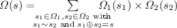
We adopt bag semantics for SPARQL: the answer to a graph pattern over an RDF graph is a multiset (or bag) of solution mappings. Formally, a bag of solution mappings is a (total) function $\varOmega$ from the set of all solution mappings to non-negative integers $\mathbb {N}$: $\varOmega (s)$ is called the multiplicity of s (we often use $s\in \varOmega$ as a shortcut for $\varOmega (s) > 0$). Following the grammar of graph patterns, we define respective operations on solution mapping bags. Solution mappings $s_1$ and $s_2$ are called compatible, written $s_1\sim s_2$, if $s_1(v) = s_2(v)$, for each $v \in \textit{dom}(s_1) \cap \textit{dom}(s_2)$, in which case $s_1\oplus s_2$ denotes a solution mapping with domain $\textit{dom}(s_1) \cup \textit{dom}(s_2)$ and such that $s_1 \oplus s_2:v \mapsto s_1(v)$, for $v \in \textit{dom}(s_1)$, and $s_1 \oplus s_2:v \mapsto s_2(v)$, for $v \in \textit{dom}(s_2)$. We also denote by $s|_L$ the restriction of s on $L\subseteq \textsf {V}$. Then the SPARQL operations are defined as follows:

• $\textsc {Filter}(\varOmega ,F) = \varOmega '$, where $\varOmega '(s) = \varOmega (s)$ if $s\in \varOmega$ and $F^s = \top$, and 0 otherwise;

• $\textsc {Union}(\varOmega _1, \varOmega _2) = \varOmega$, where $\varOmega (s) = \varOmega _1(s) + \varOmega _2(s)$;

• $\textsc {Join}(\varOmega _1,\varOmega _2) = \varOmega$, where ;

• $\textsc {Opt}(\varOmega _1, \varOmega _2, F) = \textsc {Union}(\textsc {Filter}(\textsc {Join}(\varOmega _1, \varOmega _2), F), \varOmega )$, where $\varOmega (s) = \varOmega _1(s)$ if $F^{s\oplus s_2} \ne \top$, for all $s_2\in \varOmega _2$ compatible with s, and 0 otherwise;

• $\textsc {Minus}(\varOmega _1,\varOmega _2) = \varOmega$, where $\varOmega (s) = \varOmega _1(s)$ if $\textit{dom}(s) \cap \textit{dom}(s_2) = \emptyset$, for all solution mappings $s_2\in \varOmega _2$ compatible with s, and 0 otherwise;

• $\textsc {Proj}(\varOmega , L) = \varOmega '$, where $\varOmega '(s') = \sum \limits _{s \in \varOmega \text { with }s|_L = s'} \varOmega (s)$.

Given an RDF graph G and a graph pattern P, the answer $\llbracket P\rrbracket _{G}$ to P over G is a bag of solution mappings defined by induction using the operations above and starting from basic graph patterns: $\llbracket B\rrbracket _{G}(s) = 1$ if $\textit{dom}(s) = \textit{var}(B)$ and G contains the triple s(B) obtained by replacing each variable v in B by s(v), and 0 otherwise ($\llbracket B\rrbracket _{G}$ is a set).

2.2 Relational Algebra (RA)

We recap the three-valued and bag semantics of relational algebra [13] and fix the notation. Denote by $\varDelta$ the underlying domain, which contains a distinguished element $\textit{null}$. Let U be a finite (possibly empty) set of attributes. A tuple over U is a (total) map $t:U \rightarrow \varDelta$; there is a unique tuple over $\emptyset$. A relation R over U is a bag of tuples over U, that is, a function from all tuples over U to $\mathbb {N}$. For relations $R_1$ and $R_2$ over U, we write $R_1 \subseteq R_2$ ($R_1 \equiv R_2$) if $R_1(t) \le R_2(t)$ ($R_1(t) = R_2(t)$, respectively), for all $t$.

A term v over U is an attribute $u\in U$, a constant $c\in \varDelta$ or an expression $\textit{if}(F,v,v')$, for terms v and $v'$ over U and a filter F over U. A filter F over U is a formula constructed from atoms $\textit{isNull}(V)$ and $(v=v')$, for a set V of terms and terms $v, v'$ over U, using connectives $\wedge$ and $\lnot$. Given a tuple $t$ over U, it is extended to terms as follows:

$$\begin{aligned} t(c) = c, \text { for constants } c\in \varDelta ,\qquad \text { and } \qquad t(\textit{if}(F, v,v')) = {\left\{ \begin{array}{ll}t(v), &{}\text {if } F^{t} = \top ,\\ t(v'), &{} \text {otherwise},\end{array}\right. } \end{aligned}$$

where the truth-value $F^{t} \in \{\top , \bot , \varepsilon \}$ of F on $t$ is defined inductively ($\varepsilon$ is unknown):

• $(\textit{isNull}(V))^{t}$ is $\top$ if $t(v)$ is $\textit{null}$, for all $v\in V$, and $\bot$ otherwise;

• $(v = v')^{t} =\varepsilon$ if $t(v)$ or $t(v')$ is $\textit{null}$, and the truth-value of $t(v) = t(v')$ otherwise;

• and the standard clauses for $\lnot$ and $\wedge$ in the three-valued logic (see Sect. 2.1).

We use standard abbreviations $\textit{coalesce}(v,v')$ for $\textit{if}(\lnot \textit{isNull}(v), v, v')$ and $F_1 \vee F_2$ for $\lnot (\lnot F_1\wedge \lnot F_2)$. Unlike Chebotko et al. [8], we treat $\textit{if}$ as primitive, even though the renaming operation with an $\textit{if}$ could be defined via standard operations of RA.

For filters in positive contexts, we define a weaker equivalence: filters $F_1$ and $F_2$ over U are p-equivalent, written $F_1 \!\equiv ^{\scriptscriptstyle +}\! F_2$, in case $F_1^t = \top$ iff $F_2^t = \top$, for all t over U.

We use standard relational algebra operations: union $\cup$, difference $\setminus$, projection $\pi$, selection $\sigma$, renaming $\rho$, extension $\nu$, natural (inner) join $\bowtie$ and duplicate elimination $\delta$. We say that tuples $t_1$ over $U_1$ and $t_2$ over $U_2$ are compatible² if $t_1(u) = t_2(u) \ne \textit{null}$, for all $u \in U_1 \cap U_2$, in which case $t_1 \oplus t_2$ denotes a tuple over $U_1 \cup U_2$ such that $t_1 \oplus t_2:u\mapsto t_1(u)$, for $u \in U_1$, and $t_1 \oplus t_2:u \mapsto t_2(u)$, for $u \in U_2$. For a tuple $t_1$ over $U_1$ and $U\subseteq U_1$, we denote by $t_1|_U$ the restriction of $t_1$ to U. Let $R_i$ be relations over $U_i$, for $i=1,2$. The semantics of the above operations is as follows:

• If $U_1 = U_2$, then $R_1 \cup R_2$ and $R_1 \setminus R_2$ are relations over $U_1$ satisfying $(R_1\cup R_2)(t) = R_1(t) + R_2(t)$ and $(R_1\setminus R_2)(t)\!=\!R_1(t)$ if $t\notin R_2$ and 0 otherwise;

• If $U \subseteq U_1$, then $\pi _{U}R_1$ is a relation over U with $\pi _U R_1(t) = \sum \limits _{t_1\in R_1 \text { with } t_1|_U = t} R_1(t_1)$;

• If F is a filter over $U_1$, then $\sigma _F R_1$ is a relation over $U_1$ such that $\sigma _F R_1(t)$ is $R_1(t)$ if $t\in R_1$ and $F^{t} = \top$, and 0 otherwise;

• $R_1 \!\bowtie \! R_2$ is a relation R over $U_1 {\cup }\, U_2$ such that ;

• If v is a term over $U_1$ and $u\notin U_1$ an attribute, then the extension $\nu _{u \mapsto v}R_1$ is a relation R over $U_1\cup \{u\}$ with $R(t\oplus \{ u \mapsto t(v) \}) = R_1(t)$, for all $t$. The extended projection $\pi _{\{u_1/v_1,\dots , u_k/v_k\}}$ is a shortcut for $\pi _{\{u_1,\dots ,u_k\}} \nu _{u_1\mapsto v_1}\cdots \nu _{u_k\mapsto v_k}$.

• If $v\in U_1$ and $u\notin U_1$ are distinct attributes, then the renaming $\rho _{u/v}R_1$ is a relation over $U_1\setminus \{v\} \cup \{u\}$ whose tuples t are obtained by replacing v in the domain of t by u. For terms $v_1,\dots ,v_k$ over $U_1$, attributes $u_1,\dots ,u_k$ (not necessarily distinct from $U_1$) and $V\subseteq U_1$, let $u_1',\dots ,u_k'$ be fresh attributes and abbreviate the sequence $\rho _{u_1/u'_1}\cdots \rho _{u_k/u'_k} \pi _{U_1 \cup \{u_1',\dots , u_k'\}\setminus V} \nu _{u_1' \mapsto v_1} \cdots \nu _{u_k' \mapsto v_k}$ by $\rho ^V_{\{u_1/v_1,\dots , u_k/v_k\}}$.

• $\delta R_1$ is a relation over $U_1$ with $\delta R_1(t) = \min (R_1(t), 1)$.

To bridge the gap between partial functions (solution mappings) of SPARQL and total functions (tuples) of RA, we use a padding operation: $\mu _{\{u_1, \dots , u_k\}} R_1$ denotes $\nu _{u_1\mapsto \textit{null}} \cdots \nu _{u_k\mapsto \textit{null}} R_1$, for $u_1, \dots , u_k\notin U_1$. Finally, we define the outer union, the (inner) join and left (outer) join operations by taking

note that $\bowtie _{F}$ and are natural joins: they are over F as well as shared attributes.

An RA query Q is an expression constructed from relation symbols, each with a fixed set of attributes, and filters using the RA operations (and complying with all restrictions). A data instance D gives a relation over its set of attributes, for any relation symbol. The answer to Q over D is a relation $\Vert Q\Vert _D$ defined inductively in the obvious way starting from the base case of relation symbols: $\Vert Q\Vert _D$ is the relation given by D.

3 Succinct Translation of SPARQL to SQL

We first provide a translation of SPARQL graph patterns to RA queries that improves the worst-case exponential translation of [15] in handling Join, Opt and Minus: it relies on the coalesce function (see also [7, 8]) and produces linear-size RA queries.

For any graph pattern P, the RA query $\varvec{\tau }(P)$ returns the same answers as P when solution mappings are represented as relational tuples. For a set V of variables and solution mapping s with $\textit{dom}(s)\subseteq V$, let $\textit{ext}_{V}(s)$ be the tuple over V obtained from s by padding it with $\textit{null}$s: formally,

$$\textit{ext}_{V}(s) = s\oplus \{ v\mapsto \textit{null} \mid v\in V \setminus \textit{dom}(s)\}.$$

The relational answer $\Vert P\Vert _G$ to P over an RDF graph G is a bag $\varOmega$ of tuples over $\textit{var}(P)$ such that $\varOmega (\textit{ext}_{\textit{var}(P)}(s)) = \llbracket P\rrbracket _{G}(s)$, for all solution mappings s. Conversely, to evaluate $\varvec{\tau }(P)$, we view an RDF graph G as a data instance $\textit{triple}(G)$ storing G as a ternary relation $\textit{triple}$ with the attributes $\textit{sub}$, $\textit{pred}$ and $\textit{obj}$ (note that $\textit{triple}(G)$ is a set).

The translation of a triple pattern $\langle s,p,o\rangle$ is an RA query of the form $\pi _{\dots }\sigma _F\textit{triple}$, where the subscript of the extended projection $\pi$ and filter F are determined by the variables, IRIs and literals in s, p and o; see Appendix A. SPARQL operators $\textsc {Union}$, $\textsc {Filter}$ and $\textsc {Proj}$ are translated into their RA counterparts: $\uplus$, $\sigma$ and $\pi$, respectively, with SPARQL filters translated into RA by replacing each $\textit{bound}(v)$ with $\lnot \textit{isNull}(v)$.

The translation of $\textsc {Join}$, $\textsc {Opt}$ and $\textsc {Minus}$ is more elaborate and requires additional notation. Let $P_1$ and $P_2$ be graph patterns with $U_i = \textit{var}(P_i)$, for $i = 1,2$, and denote by U their shared variables, $U_1\cap U_2$. To rename the shared attributes apart, we introduce fresh attributes $u^1$ and $u^2$ for each $u\in U$, set $U^i = \{ u^i \mid u \in U\}$ and use abbreviations $U^i/U$ and $U/U^i$ for $\{u^i / u \mid \, u \in U\}$ and $\{u / u^i \mid u \in U\}$, respectively, for $i = 1,2$. Now we can express the SPARQL solution mapping compatibility:

$$\begin{aligned} \textit{comp}_U \ \ = \ \bigwedge \nolimits _{u\in U} \bigl [(u^1 = u^2) \vee \textit{isNull}(u^1) \vee \textit{isNull}(u^2)\bigr ] \end{aligned}$$

(intuitively, the $\textit{null}$ value of an attribute in the context of RA queries represents the fact that the corresponding SPARQL variable is not bound). Next, the renamed apart attributes need to be coalesced to provide the value in the representation of the resulting solution mapping; see $\oplus$ in Sect. 2.1. To this end, given an RA filter F over a set of attributes V, terms $v_1,\dots ,v_k$ over V and attributes $u_1,\dots ,u_k\notin V$, we denote by $F[u_1/v_1,\dots , u_k/v_k]$ the result of replacing each $u_i$ by $v_i$ in F. We also denote by $\textit{coalesce}_U$ the substitution of each $u\in U$ with $\textit{coalesce}(u^1,u^2)$; thus, $F[\textit{coalesce}_U]$ is the result of replacing each $u\in U$ in F with $\textit{coalesce}(u^1,u^2)$. We now set

where $w\notin U_1 \cup U_2$ is an attribute and $1\in \varDelta \setminus \{\textit{null} \}$ is any domain element. The translation of $\textsc {Join}$ and $\textsc {Opt}$ is straightforward. For $\textsc {Minus}$, observe that $\nu _{w\mapsto 1}$ extends the relation for $P_2$ by a fresh attribute w with a non-$\textit{null}$ value. The join condition encodes compatibility of solution mappings whose domains, in addition, share a variable (both $u^1$ and $u^2$ are non-$\textit{null}$). Tuples satisfying the condition are then filtered out by $\sigma _{\textit{isNull}(w)}$, leaving only representations of solution mappings for $P_1$ that have no compatible solution mapping in $P_2$ with a shared variable. Finally, the attributes are renamed back by $\rho _{U/U^1}$ and unnecessary attributes are projected out by $\pi _{U_1}$.

Theorem 3

For any RDF graph G and any graph pattern P, $\Vert P\Vert _G = \Vert \varvec{\tau }(P)\Vert _{\textit{triple}(G)}.$

The complete proof of Theorem 3 can be found in Appendix A.

4 Optimisations of Translated SPARQL Queries

We present optimisations on a series of examples. We begin by revisiting Example 1, which can now be given in algebraic form (for brevity, we ignore projecting away ?p, which does not affect any of the optimisations discussed):

$$\begin{aligned} \textsc {Opt}(\textsc {Opt}(\texttt {?p :name ?n}, \ \ \texttt {?p :workEmail ?e}, \ \ \top ), \texttt {?p :personalEmail ?e}, \ \ \top ), \end{aligned}$$

where $\top$ denotes the tautological filter (true). Suppose we have the mapping

$$\begin{aligned} \textsc {iri}_1(\texttt {id}) \ \ \texttt {:name} \ \ \texttt {fullName}&\ \ \leftarrow \ \ \sigma _{\lnot \textit{isNull}(\texttt {id}) \wedge \lnot \textit{isNull}(\texttt {fullName})}{} \texttt {people}, \\ \textsc {iri}_1(\texttt {id}) \ \ \texttt {:workEmail} \ \ \texttt {workEmail}&\ \ \leftarrow \ \ \sigma _{\lnot \textit{isNull}(\texttt {id}) \wedge \lnot \textit{isNull}(\texttt {workEmail})}\,\texttt {people},\\ \textsc {iri}_1(\texttt {id}) \ \ \texttt {:personalEmail} \ \ \texttt {homeEmail}&\ \ \leftarrow \ \ \sigma _{\lnot \textit{isNull}(\texttt {id}) \wedge \lnot \textit{isNull}(\texttt {homeEmail})}\,\texttt {people}, \end{aligned}$$

where $\textsc {iri}_1$ is a function that constructs the IRI for a person from their ID (an IRI template, in R2RML parlance). We assume that the IRI functions are injective and map only $\textit{null}$ to $\textit{null}$; thus, joins on $\textsc {iri}_1(\texttt {id})$ can be reduced to joins on $\texttt {id}$, and $\textit{isNull}(\texttt {id})$ holds just in case $\textit{isNull}(\textsc {iri}_1(\texttt {id}))$ holds. Interestingly, the IRI functions can encode GLAV mappings, where the target query is a full-fledged CQ (in contrast to GAV mappings, where atoms do not contain existential variables); for more details, see [10].

The translation given in Sect. 3 and unfolding produce the following RA query, where we abbreviate, for example, $\rho ^{\{p^1, p^2\}}_{\{p^4/\textit{coalesce}(p^1,p^2)\}}$ by $\bar{\rho }_{\{p^4/\textit{coalesce}(p^1,p^2)\}}$ (in other words, the $\bar{\rho }$ operation always projects away the arguments of its $\textit{coalesce}$ functions):

In our diagrams, the white nodes are the contribution of the mapping and the translation of the basic graph patterns: for example, the basic graph pattern ?p :name ?n produces $\smash {\pi _{\{p^1/\textsc {iri}_1(\texttt {id}),\ n/\texttt {fullName}\}}\sigma _{\lnot \textit{isNull}(\texttt {id}) \wedge \lnot \textit{isNull}(\texttt {fullName})}}{} \texttt {people}$ (we use attributes without superscripts if there is only one occurrence; otherwise, the superscript identifies the relevant subquery). The grey nodes correspond to the translation of the SPARQL operations: for instance, the innermost left join is on $\smash {\textit{comp}_{\{p\}}}$ with p renamed apart to $\smash {p^1}$ and $\smash {p^2}$; the outermost left join is on $\smash {\textit{comp}_{\{p, e\}}}$, where p is renamed apart to $\smash {p^4}$ and $\smash {p^3}$ and e to $\smash {e^2}$ and $\smash {e^3}$; the two $\bar{\rho }$ are the respective renaming operations with $\textit{coalesce}$.

4.1 Compatibility Filter Reduction (CFR)

We begin by simplifying the filters in (left) joins and eliminating renaming operations with $\textit{coalesce}$ above them (if possible). First, we can pull up the filters of the mapping through the extended projection and union by means of standard database equivalences: for example, for relations $R_1$ and $R_2$ and a filter F over U, we have $\sigma _F(R_1 \cup R_2) \equiv \sigma _F R_1 \cup \sigma _F R_2$, and $\pi _{U'} \sigma _{F'} R_1 \equiv \sigma _{F'} \pi _{U'} R_1$, if $F'$ is a filter over $U' \subseteq U$, and $\rho _{u/v} \sigma _F R_1 \equiv \sigma _{F[u/v]} \rho _{u/v} R_1$, if $v \in U$ and $u\notin U$.

Second, the filters can be moved (in a restricted way) between the arguments of a left join to its join condition: for relations $R_1$ and $R_2$ over $U_1$ and $U_2$, respectively, and filters $F_1$, $F_2$ and F over $U_1$, $U_2$ and $U_1 \cup U_2$, respectively, we have

(1)

(2)

(3)

observe that unlike $\sigma _{F_2}$ in (3), the selection $\sigma _{F_1}$ cannot be entirely eliminated in (2) but can rather be ‘duplicated’ above the left join using (1). (We note that (1) and (3) are well-known and can be found, e.g., in [12].) Simpler equivalences hold for inner join: $\sigma _{F_1} R_1 \bowtie _F R_2 \equiv \sigma _{F\wedge F_1} (R_1 \bowtie R_2)$. These equivalences can be, in particular, used to pull up the $\lnot \textit{isNull}$ filters from mappings to eliminate the $\textit{isNull}$ disjuncts in the compatibility condition $\textit{comp}_U$ of the (left) joins in the translation by means of the standard p-equivalences of the three-valued logic:

$$\begin{aligned} (F_1 \vee F_2) \wedge \lnot F_2&\ \ \equiv ^{\scriptscriptstyle +} \ \ F_1 \wedge \lnot F_2, \end{aligned}$$

(4)

$$\begin{aligned} (v = v') \wedge \lnot \textit{isNull}(v)&\ \ \equiv ^{\scriptscriptstyle +} \ \ (v = v'); \end{aligned}$$

(5)

we note in passing that this step refines Simplification 3 of Chebotko et al. [8], which relies on the absence of other left joins in the arguments of a (left) join.

Third, the resulting simplified compatibility conditions can eliminate $\textit{coalesce}$ from the renaming operations: for a relation R over U and $u^1, u^2\in U$, we clearly have

$$\begin{aligned} \rho ^{\{u^1, u^2\}}_{\{u/\textit{coalesce}(u^1,u^2)\}} \sigma _{\lnot \textit{isNull}(u^1)} R \ \ \ \equiv \ \ \ \sigma _{\lnot \textit{isNull}(u)} \pi _{U\setminus \{u^2\}} R[u/u^1], \end{aligned}$$

(6)

where $R[u/u^1]$ is the result of replacing each $u^1$ in R by u. This step generalises Simplification 2 of Chebotko et al. [8], which does not eliminate $\textit{coalesce}$ above (left) joins that contain nested left joins.

By applying these three steps to our running example, we obtain (see Appendix C.1)

4.2 Left Join Naturalisation (LJN)

Our next group of optimisations can remove join conditions in left joins (if their arguments satisfy certain properties), thus reducing them to natural left joins.

Some equalities in the join conditions of left joins can be removed by means of attribute duplication: for relations $R_1$ and $R_2$ over $U_1$ and $U_2$, respectively, a filter F over $U_1\cup U_2$ and attributes $u^1 \in U_1\setminus U_2$ and $u^2 \in U_2 \setminus U_1$, we have

(7)

Now, the duplicated $u^2$ can be eliminated in case it is actually projected away:

(8)

So, if F is a conjunction of suitable attribute equalities, then by repeated application of (7) and (8), we can turn a left join into a natural left join. In our running example, this procedure simplifies the innermost left join to

Another technique for converting a left join into a natural left join ( is just an abbreviation for ) is based on the conditional function $\textit{if}$:

Proposition 4

For relations $R_1$ and $R_2$ over $U_1$ and $U_2$, respectively, and a filter F over $U_1 \cup U_2$, we have

(9)

Proof

Denote $R_1\bowtie R_2$ by S. Then $\pi _{U_1} S \subseteq R_1$ implies that every tuple $t_1$ in $R_1$ can have at most one tuple $t_2$ in $R_2$ compatible with it, and S consists of all such extensions (with their cardinality determined by $R_1$). Therefore, $\pi _{U_1}(S \setminus \sigma _F S)$ is precisely the tuples in $R_1$ that cannot be extended in such a way that the extension satisfies F, whence

$$\begin{aligned} \pi _{U_1}(S \setminus \sigma _F S)&\ \ \equiv \ \ \pi _{U_1}S \setminus \pi _{U_1}\sigma _F S. \end{aligned}$$

(10)

By a similar argument, $R_1 \setminus \pi _{U_1} S$ consists of the tuples in $R_1$ (with the same cardinality) that cannot be extended by a tuple in $R_2$, and $\pi _{U_1} S \setminus \pi _{U_1} \sigma _F S$ of those tuples that can be extended but only when F is not satisfied. By taking the union of the two, we obtain

$$\begin{aligned} (R_1 \setminus \pi _{U_1} S) \ \ \cup \ \ (\pi _{U_1} S \setminus \pi _{U_1} \sigma _F S)&\ \ \equiv \ \ R_1 \setminus \pi _{U_1} \sigma _F S. \end{aligned}$$

(11)

The claim is then proved by distributivity of $\rho$ and $\mu$ over $\cup$; see Appendix B.

Proposition 4 is, in particular, applicable if the attributes shared by $R_1$ and $R_2$ uniquely determine tuples of $R_2$. In our running example, $\texttt {id}$ is a primary key in $\texttt {people}$, and so we can eliminate $\lnot \textit{isNull}(e^2)$ from the innermost left join, which becomes a natural left join, and then simplify the term $\textit{if}(\lnot \textit{isNull}(e^2), e^2, \textit{null})$ in the renaming to $e^2$ by using equivalences on complex terms: for a term v and a filter F over U, we have

$$\begin{aligned} \textit{if}(F \wedge \lnot \textit{isNull}(v), v, \textit{null})&\ \ \equiv \ \ \textit{if}(F, v, \textit{null}),\end{aligned}$$

(12)

$$\begin{aligned} \textit{if}(\top , v, \textit{null})&\ \ \equiv \ \ v. \end{aligned}$$

(13)

Thus, we effectively remove the renaming operator introduced by the application of Proposition 4; for full details, see Appendix C.1.

4.3 Translation for Well-Designed SPARQL

We remind the reader that a SPARQL pattern P that uses only $\textsc {Join}$, $\textsc {Filter}$ and binary $\textsc {Opt}$ (that is, $\textsc {Opt}$ with the tautological filter $\top$) is well-designed [16] if every its subpattern $P'$ of the form $\textsc {Opt}(P_1, P_2, \top )$ satisfies the following condition: every variable u that occurs in $P_2$ and outside $P'$ also occurs in $P_1$.

Proposition 5

If P is well-designed, then its unfolded translation can be equivalently simplified by (a) removing all compatibility filters $\textit{comp}_U$ from joins and left joins and (b) eliminating all renamings $u/\textit{coalesce}(u^1,u^2)$ by replacing both $u^1$ and $u^2$ with u.

Proof

Since P is well-designed, any variable u occurring in the right-hand side argument of any $\textsc {Opt}$ either does not occur elsewhere (and so, can be projected away) or also occurs in the left-hand side argument. The claim then follows from an observation that, if the translation of $P_1$ or $P_2$ can be equivalently transformed to contain a selection with $\lnot \textit{isNull}(u)$ at the top, then the translation of $\textsc {Join}(P_1, P_2)$, $\textsc {Opt}(P_1, P^*, \top )$ and $\textsc {Filter}(P_1,F)$ can also be equivalently simplified so that it contains a selection with the $\lnot \textit{isNull}(u^1)$ or, respectively, $\lnot \textit{isNull}(u^2)$ condition at the top.

Rodríguez-Muro and Rezk [22] made a similar observation. Alas, Example 1 shows that Proposition 5 is not directly applicable to weakly well-designed SPARQL [14].

4.4 Natural Left Join Reduction (NJR)

A natural left join can then be replaced by a natural inner join if every tuple of its left-hand side argument has a match on the right, which can be formalised as follows.

Proposition 6

For relations $R_1$ and $R_2$ over $U_1$ and $U_2$, respectively, we have

(14)

Proof

By careful inspection of definitions. Alternatively, one can assume that the left join has an additional selection on top with filters of the form $(u^1 = u^2) \vee \textit{isNull}(u^2)$, for $u\in K$, where $u^1$ and $u^2$ are duplicates of attributes from $R_1$ and $R_2$, respectively. Given $\delta \pi _K R_1 \subseteq \pi _K R_2$, one can eliminate the $\textit{isNull}(u^2)$ because any tuple of $R_1$ has a match in $R_2$. The resulting $\textit{null}$-rejecting filter then effectively turns the left join to an inner join by the outer join simplification of Galindo-Legaria and Rosenthal [12].

Observe that the inclusion $\delta \pi _K R_1 \subseteq \pi _K R_2$ is satisfied, for example, if $R_1$ has a foreign key K referencing $R_2$. It can also be satisfied if both $R_1$ and $R_2$ are based on the same relation, that is, $R_i \equiv \sigma _{F_i}\pi _{\dots } R$, for $i = 1,2$, and $F_1$ logically implies $F_2$, where $F_1$ and/or $F_2$ can be $\top$ for the vacuous selection. Note that, due to $\delta$, attributes K do not have to uniquely determine tuples in $R_1$ or $R_2$. In our running example, trivially, $\delta \pi _{\{p\}} (\pi _{\{p/\textsc {iri}_1(\texttt {id}),\ n/\texttt {fullName}\}} \texttt {people}) \ \ \subseteq \ \ \pi _{\{p\}} (\pi _{\{p/\textsc {iri}_1(\texttt {id}),\ e^2/\texttt {workEmail}\}} \texttt {people})$. Therefore, the inner left join can be replaced by a natural inner join, which can then be eliminated altogether because id is the primary key in people (this is a well-known optimisation; see, e.g., [11, 21]). As a result, we obtain

The running example is wrapped up and discussed in detail in Appendices C.1 and C.2.

4.5 Join Transfer (JT)

To introduce and explain another optimisation, we need an extension of relation people with a nullable attribute spouseId, which contains the id of the person’s spouse if they are married and NULL otherwise. The attribute is mapped by an additional assertion:

$$\begin{aligned} \textsc {iri}_1(\texttt {id}) \ \ \texttt {:hasSpouse} \ \ \textsc {iri}_1(\texttt {spouseId}) \quad \leftarrow \quad \sigma _{\lnot \textit{isNull}(\texttt {id}) \wedge \lnot \textit{isNull}(\texttt {spouseId})}{} \texttt {people}. \end{aligned}$$

Consider now the following query in SPARQL algebra:

$$\begin{aligned} \textsc {Proj}(\textsc {Opt}(\texttt {?p :name ?n}, \textsc {Join}(\texttt {?p :hasSpouse ?s},\ \texttt {?s :name ?sn}), \top ), \{\,\texttt {?n}, \texttt {?sn} \,\}), \end{aligned}$$

whose translation can be unfolded and simplified with optimisations in Sects. 4.1 and 4.2 into the following RA query (we have also pushed down the filter $\lnot \textit{isNull}(sn)$ to the right argument of the join and, for brevity, omitted selection and projection at the top):

see Appendix C.4 for full details. Observe that the inner join cannot be eliminated using the standard self-join elimination techniques because it is not on a primary (or alternate) key. The next proposition (proved in Appendix B) provides a solution for the issue.

Proposition 7

Let $R_1$, $R_2$ and $R_3$ be relations over $U_1$, $U_2$ and $U_3$, respectively, F a filter over $U_1\cup U_2 \cup U_3$ and w an attribute in $U_3 \setminus (U_1 \cup U_2)$. Then

(15)

By Proposition 7, we take sn as the non-nullable attribute w and get the following:

Now, the inner self-join can be eliminated (as id is the primary key of people) and the $\rho$ operation removed (as its result is projected away); see Appendix C.4.

4.6 Left Join Decomposition (LJD): Left Join Simplification [12] Revisited

In Sect. 4.4, we have given an example of a reduction of a left join to an inner join. The following equivalence is also helpful (for an example, see Appendix C.3): for relations $R_1$ and $R_2$ over $U_1$ and $U_2$, respectively, and a filter F over $U_1\cup U_2$,

(16)

Galindo-Legaria and Rosenthal [12] observe that  whenever G rejects $\textit{null}$s on $U_2\setminus U_1$. In the context of SPARQL, however, the compatibility condition $\textit{comp}_U$ does not satisfy the $\textit{null}$-rejection requirement, and so, this optimisation is often not applicable. In the rest of this section we refine the basic idea.

Let $R_1$ and $R_2$ be relations over $U_1$ and $U_2$, respectively, and F and G filters over $U_1 \cup U_2$. It can easily be verified that, in general, we can decompose the left join:

(17)

where $\textit{nullify}_{U_2\setminus U_1}(G)$ is the result of replacing every occurrence of an attribute from $U_2\setminus U_1$ in G with $\textit{null}$. Observe that if G is $\textit{null}$-rejecting on $U_2\setminus U_1$, then $\textit{nullify}_{U_2\setminus U_1}(G)\equiv ^{\scriptscriptstyle +}\bot$, and the second component of the union in (17) is empty. We, however, are interested in a subtler interaction of the filters when the second component of the difference or, respectively, the first component of the union is empty:

(18)

(19)

These cases are of particular relevance for the SPARQL-to-SQL translation of OPTIONAL and MINUS. We illustrate the technique in Appendix C.5 on the following example:

$$\begin{aligned}&\textsc {Filter}(\textsc {Opt}(\textsc {Opt}(\texttt {?p a :Product}, \\& \textsc {Filter}(\texttt {\{ ?p :hasReview ?r . ?r :hasLang ?l \}}, \texttt {?l} = \texttt {"en"}), \ \top ),\\& \textsc {Filter}(\texttt {\{ ?p :hasReview ?r . ?r :hasLang ?l \}}, \texttt {?l} = \texttt {"zh"}), \ \top ),\ \textit{bound}(\texttt {?r})). \end{aligned}$$

The technique relies on two properties of $\textit{null}$ propagation from the right-hand side of left joins. Let $R_1$ and $R_2$ be relations over $U_1$ and $U_2$, respectively. First, if $v = v'$ is a left join condition and v is a term over $U_2\setminus U_1$, then v is either $\textit{null}$ or $v'$ in the result:

(20)

Second, non-nullable terms $v, v'$ over $U_2\setminus U_1$ are simultaneously either $\textit{null}$ or not $\textit{null}$:

(21)

The two equivalences introduce no new filters apart from $\textit{isNull}$ and their negations. The introduced filters, however, can help simplify the join conditions of the left joins containing the left join under consideration.

5 Experiments

In order to verify effectiveness of our optimisation techniques, we carried out a set of experiments based on the BSBM benchmark [3]; the materials for reproducing the experiments are available online³. The BSBM benchmark is built around an e-commerce use case in which vendors offer products that can be reviewed by customers. It comes with a mapping, a data generator and a set of SPARQL and equivalent SQL queries.

Hardware and Software. The experiments were performed on a t2.xlarge Amazon EC2 instance with four 64-bit vCPUs, 16G memory and 500G SSD hard disk under Ubuntu 16.04LTS. We used five database engines: free MySQL 5.7 and PostgreSQL 9.6 are run normally, and 3 commercial systems (which we shall call X, Y and Z) in Docker.

Queries. In total, we consider 11 SPARQL queries. Queries Q1–Q4 are based on the original BSBM queries 2, 3, 7 and 8, which contain OPTIONAL; we modified them to reduce selectivity: e.g., Q1, Q3 and Q4 retrieve information about 1000 products rather than a single product in the original BSBM queries; we also removed ORDER BY and LIMIT clauses. Q1–Q4 are well-designed (WD). In addition, we created 7 weakly well-designed (WWD) SPARQL queries: Q5–Q7 are similar to Example 1, Q8–Q10 to the query in Sect. 4.6, and Q11 is along the lines of Sect. 4.5. More information is below:

Query	Description	SPARQL	Optimisations
Q1	2 simple OPTIONALs for the padding effect (derived from BSBM query 2)	WD	LJN, NLJR
Q2	1 OPTIONAL with a !BOUND filter (encodes MINUS) derived from BSBM query 3	WD	JT
Q3	2 outer-level OPTIONALs, the latter with 2 nested OPTIONALs derived from BSBM query 7	WD	LJN, NLJR
Q4	4 OPTIONALs: ratings from attributes of the same relation derived from BSBM query 8	WD	LJN, NLJR
Q5/6/7	2/3/4 OPTIONALs: preference over 2/3/4 ratings of reviews	WWD	LJN, NLJR
Q8/9/10	2/3/4 OPTIONALs: preference of reviews over 2/3/4 languages	WWD	LJN, LJD
Q11	2 OPTIONALs: country-based preference of home pages of reviewed products	WWD	LJN, NLJR, JT

Data. We used the BSBM generator to produce CSV files for 1M products and 10M reviews. The CSV files (20GB) were loaded into DBs, with the required indexes created.

Evaluation. For each SPARQL query, we computed two SQL translations. The non-optimised (N/O) translation is obtained by applying to the unfolded query only the standard (previously known and widely adopted) structural and semantic optimisations [4] as well as CFR (Sect. 4.1) to simplify compatibility filters and eliminate unnecessary COALESCE. To obtain the optimised (O) translations, we further applied the other optimisation techniques presented in Sect. 4 (as described in the table above). We note that the optimised Q1 and Q4 have the same structure as the SQL queries in the original benchmark suite. On the other hand, the optimised Q2 is different from the SQL query in BSBM because the latter uses (NOT) IN, which is not considered in our optimisations.

Each query was executed three times with cold runs to avoid any variation due to caching. The size of query answers and their running times (in secs) are as follows:

Query	# answers	PostgreSQL		MySQL		X		Y		Z
		N/O	O	N/O	O	N/O	O	N/O	O	N/O	O
Q1	19,267	1.79	1.77	0.43	0.38	0.90	0.80	0.56	0.52	29.06	25.09
Q2	6,746	18.75	2.07	19.95	0.36	40.00	16.07	0.44	0.37	27.99	5.97
Q2bsbm			3.88		0.37		20.55		0.38		5.91
Q3	1,355	4.20	0.09	4.70	0.11	5.50	1.60	2.04	0.14	5.45	0.65
Q4	1,174	2.14	0.16	0.86	0.04	3.00	0.60	1.78	0.11	4.38	0.53
Q5	2,294	0.56	0.05	0.01	0.01	1.80	0.30	0.30	0.08	0.51	0.53
Q6	2,294	102.35	0.18	>10 min	0.04	1.90	0.40	4.50	0.14	0.82	0.54
Q7	2,294	102.00	0.17	>10 min	0.04	2.60	0.40	14.57	0.14	1.21	0.53
Q8	1,257	0.07	0.06	0.01	0.01	8.40	1.30	0.08	0.08	295.25	0.40
Q9	1,311	101.20	0.16	>10 min	0.04	>10 min	2.70	4.30	0.11	>10 min	0.43
Q10	1,331	103.30	0.15	>10 min	0.05	>10 min	4.20	5.20	0.14	>10 min	0.43
Q11	3,388	5.26	0.87	3.80	0.21	107.06	2.68	177.95	0.22	7.82	0.13

The main outcomes of our experiments can be summarised as follows.

• (a) The running times confirm that the optimisations are effective for all database engines. All optimised translations show better performance in all DB engines, and most of them can be evaluated in less than a second.

• (b) Interestingly, our optimised translation is even slightly more efficient than the SQL with (NOT) IN from the original BSBM suite (see Q2bsbm in the table).

• (c) The effects of the optimisations are significant. In particular, for challenging queries (some of which time out after 10 min), it can be up to three orders of magnitude.

6 Discussion and Conclusions

The optimisation techniques we presented are intrinsic to SQL queries obtained by translating SPARQL in the context of OBDA with mappings, and their novelty is due to the interaction of the components in the OBDA setting. Indeed, the optimisation of LEFT JOINs can be seen as a form of “reasoning” on the structure of the query, the data source and the mapping. For instance, when functional and inclusion dependencies along with attribute nullability are taken into account, one may infer that every tuple from the left argument of a LEFT JOIN is guaranteed to match (i) at least one or (ii) at most one tuple on the right. This information can allow one to replace LEFT JOIN by a simpler operator such as an INNER JOIN, which can further be optimised by the known techniques.

Observe that, in normal SQL queries, most of the NULLs come from the database rather than from operators like LEFT JOIN. In contrast, SPARQL triple patterns always bind their variables (no NULLs), and only operators like OPTIONAL can “unbind” them. In our experiments, we noticed that avoiding the padding effect is probably the most effective outcome of the LEFT JOIN optimisation techniques in the OBDA setting.

From the Semantic Web perspective, our optimisations exploit information unavailable in RDF triplestores, namely, database integrity constraints and mappings. From the DB perspective, we believe that such techniques have not been developed because LEFT JOINs and/or complex conditions like compatibility filters are not introduced accidentally in expert-written SQL queries. The results of our evaluation support this hypothesis and show a significant performance improvement, even for commercial DBMSs.

We are working on implementing these techniques in the OBDA system Ontop [4].

References

Arias, M., Fernández, J.D., Martínez-Prieto, M.A., de la Fuente, P.: An empirical study of real-world SPARQL queries. In: Proceedings of USEWOD (2011)
Atre, M.: Left bit right: for SPARQL join queries with OPTIONAL patterns (left-outer-joins). In: Proceedings of ACM SIGMOD, pp. 1793–1808 (2015)
Bizer, C., Schultz, A.: The Berlin SPARQL benchmark. Int. J. Semant. Web Inf. Syst. 5(2), 1–24 (2009)
Calvanese, D., Cogrel, B., Komla-Ebri, S., Kontchakov, R., Lanti, D., Rezk, M., Rodriguez-Muro, M., Xiao, G.: Ontop: answering SPARQL queries over relational databases. SWJ 8, 471–487 (2017)
Calvanese, D., De Giacomo, G., Lembo, D., Lenzerini, M., Rosati, R.: Tractable reasoning and efficient query answering in description logics: the DL-Lite family. JAR 39, 385–429 (2007)
Chakravarthy, U.S., Grant, J., Minker, J.: Logic-based approach to semantic query optimization. ACM TODS 15(2), 162–207 (1990)
Chaloupka, M., Nečaský, M.: Efficient SPARQL to SQL translation with user defined mapping. In: Ngonga Ngomo, A.-C., Křemen, P. (eds.) KESW 2016. CCIS, vol. 649, pp. 215–229. Springer, Cham (2016). https://doi.org/10.1007/978-3-319-45880-9_17
Chebotko, A., Lu, S., Fotouhi, F.: Semantics preserving SPARQL-to-SQL translation. DKE 68(10), 973–1000 (2009)
Cyganiak, R.: A relational algerba for SPARQL. TR HPL-2005-170, HP Labs Bristol (2005)
De Giacomo, G., Lembo, D., Lenzerini, M., Poggi, A., Rosati, R.: Using ontologies for semantic data integration. In: Flesca, S., Greco, S., Masciari, E., Saccà, D. (eds.) A Comprehensive Guide Through the Italian Database Research Over the Last 25 Years. SBD, vol. 31, pp. 187–202. Springer, Cham (2018). https://doi.org/10.1007/978-3-319-61893-7_11
Elmasri, R., Navathe, S.: Fundamentals of Database Systems. Addison-Wesley, Boston (2010)
Galindo-Legaria, C., Rosenthal, A.: Outerjoin simplification and reordering for query optimization. ACM TODS 22(1), 43–74 (1997)
Guagliardo, P., Libkin, L.: A formal semantics of SQL queries, its validation, and applications. PVLDB 11(1), 27–39 (2017)
Kaminski, M., Kostylev, E.V.: Beyond well-designed SPARQL. In: Proceedings of ICDT (2016)
Kontchakov, R., Rezk, M., Rodríguez-Muro, M., Xiao, G., Zakharyaschev, M.: Answering SPARQL queries over databases under OWL 2 QL entailment regime. In: Mika, P., et al. (eds.) ISWC 2014. LNCS, vol. 8796, pp. 552–567. Springer, Cham (2014). https://doi.org/10.1007/978-3-319-11964-9_35
Pérez, J., Arenas, M., Gutierrez, C.: Semantics and complexity of SPARQL. ACM TODS 34(3), 16:1–16:45 (2009)
Picalausa, F., Vansummeren, S.: What are real SPARQL queries like? In: SWIM (2011)
Poggi, A., Lembo, D., Calvanese, D., De Giacomo, G., Lenzerini, M., Rosati, R.: Linking data to ontologies. J. Data Semant. 10, 133–173 (2008)
Priyatna, F., Corcho, Ó., Sequeda, J.F.: Formalisation and experiences of R2RML-based SPARQL to SQL query translation using morph. In: Proceedings of WWW, pp. 479–490 (2014)
Rao, J., Pirahesh, H., Zuzarte, C.: Canonical abstraction for outerjoin optimization. In: Proceedings of ACM SIGMOD, pp. 671–682 (2004)
Rodríguez-Muro, M., Kontchakov, R., Zakharyaschev, M.: Ontology-based data access: Ontop of databases. In: Alani, H. (ed.) ISWC 2013. LNCS, vol. 8218, pp. 558–573. Springer, Heidelberg (2013). https://doi.org/10.1007/978-3-642-41335-3_35
Rodriguez-Muro, M., Rezk, M.: Efficient SPARQL-to-SQL with R2RML mappings. J. Web Semant. 33, 141–169 (2015)
Schmidt, M., Meier, M., Lausen, G.: Foundations of SPARQL query optimization. In: Proceedings ICDT, pp. 4–33 (2010)
Sequeda, J.F., Arenas, M., Miranker, D.P.: OBDA: query rewriting or materialization? In practice, both!. In: Mika, P., et al. (eds.) ISWC 2014. LNCS, vol. 8796, pp. 535–551. Springer, Cham (2014). https://doi.org/10.1007/978-3-319-11964-9_34
Acknowledgements
We thank the reviewers for their suggestions. This work was supported by the OBATS project at the Free University of Bozen-Bolzano and by the Euregio (EGTC) IPN12 project KAOS.
Author information
Authors and Affiliations
Corresponding author
Editor information
Editors and Affiliations
Rights and permissions
Copyright information
© 2018 Springer Nature Switzerland AG
About this paper
Cite this paper
Xiao, G., Kontchakov, R., Cogrel, B., Calvanese, D., Botoeva, E. (2018). Efficient Handling of SPARQL OPTIONAL for OBDA. In: Vrandečić, D., et al. The Semantic Web – ISWC 2018. ISWC 2018. Lecture Notes in Computer Science(), vol 11136. Springer, Cham. https://doi.org/10.1007/978-3-030-00671-6_21
Download citation
DOI: https://doi.org/10.1007/978-3-030-00671-6_21
Published:
Publisher Name: Springer, Cham
Print ISBN: 978-3-030-00670-9
Online ISBN: 978-3-030-00671-6
eBook Packages: Computer ScienceComputer Science (R0)