PSPACE-Completeness of the Soundness Problem of Safe Asymmetric-Choice Workflow Nets

Abstract

Asymmetric-choice workflow nets (ACWF-nets) are an important subclass of workflow nets (WF-nets) that can model and analyse business processes of many systems, especially the interactions among multiple processes. Soundness of WF-nets is a basic property guaranteeing that these business processes are deadlock-/livelock-free and each designed action has a potential chance to be executed. Aalst et al. proved that the soundness problem is decidable for general WF-nets and proposed a polynomial algorithm to check the soundness for free-choice workflow nets (FCWF-nets) that are a special subclass of ACWF-nets. Tiplea et al. proved that for safe acyclic WF-nets the soundness problem is co-NP-complete, and we proved that for safe WF-nets the soundness problem is PSPACE-complete. We also proved that for safe ACWF-nets the soundness problem is co-NP-hard, but this paper sharpens this result by proving that for safe ACWF-nets this problem is PSPACE-complete actually. This paper provides a polynomial-time reduction from the acceptance problem of linear bounded automata (LBA) to the soundness problem of safe ACWF-nets. The kernel of the reduction is to guarantee that an LBA with an input string does not accept the input string if and only if the constructed safe ACWF-net is sound. Based on our reduction, we easily prove that the liveness problem of safe AC-nets is also PSPACE-complete, but the best result on this problem was NP-hardness provided by Ohta and Tsuji. Therefore, we also strengthen their result.

1 Introduction

Workflow nets (WF-nets) have been widely applied to the modelling and analysis of business process management systems [1,2,3, 21,22,23,24, 38]. To satisfy more design or analysis requirements, some extensions are proposed such as WFD-nets (workflow nets with data) [33, 36], WFT-nets (workflow nets with tables) [30] and PWNs (probabilistic workflow nets) [11, 27]. All of them use WF-nets to model execution logics of business processes including sequence, choice, loop, concurrence and/or interaction.

Soundness [1,2,3] is an important property required by these systems. Different types of models generally give different notions of soundness [30, 33], and even for classical WF-nets, there are different notions of soundness [3]. But most of them require that business processes have neither deadlock nor livelock and every designed action has a potential executed chance. This paper considers this classical notion of soundness.

It has been proven that the soundness problem is decidable and EXPSPACE-hard for general WF-nets [2, 21, 34]. These results are based on the fact that the problems of reachability¹, liveness, and deadlock of Petri nets are all EXPSPACE-hard [8, 14]. Aalst [2] provided a polynomial-time algorithm to solve the soundness problem for free-choice WF-nets. For safe WF-nets we proved that this problem is PSPACE-complete [20]; and for safe acyclic WF-nets Tiplea et al. proved that this problem is co-NP-complete [32].

Asymmetric-choice workflow nets (ACWF-nets) [37] are an important subclass of WF-nets. Not only that, asymmetric-choice nets (AC-nets) [4, 10] are also an important subclass of Petri nets. AC-nets not only own a stronger modelling power rather than their subclass FC-nets (free-choice nets), but also their special structures play an important role in analysing their properties such as liveness [5, 10, 15], response property [25] and system synthesis [35]. Free-choice structures can hardly model the interactions of multiple processes, while asymmetric-choice structures can usually handle them [1, 19, 26]. But so far, there are not too much theoretical results of complexity of deciding properties for AC-nets or ACWF-nets, and the existing ones are not too accurate, e.g. Ohta and Tsuji proved that the liveness problem of safe AC-nets is NP-hard [28], and we proved that the soundness problem of safe ACWF-nets is co-NP-hard [18].

Table 1. Complexity results for some subclasses.

Contributions. This paper sharpens these results by proving that the soundness problem of safe ACWF-nets and the liveness problem of safe AC-nets are both PSPACE-complete. We can construct a safe ACWF-net for any linear bounded automaton (LBA) with an input string by the following idea: if an LBA with an input string accepts the string, the constructed safe ACWF-net is not sound; if it does not accept the string, the constructed safe ACWF-net is sound. In addition, based on the PSPACE-completeness of the soundness problem of safe ACWF-nets and the equivalence between the soundness problem and the liveness and boundedness problem in WF-nets [2], we can infer that the liveness problem of safe AC-nets is PSPACE-complete. We also show that the reachability problem of safe AC-nets is PSPACE-complete.

The complexity results of reachability, liveness and soundness for some subclasses of Petri nets are summarised in Table 1 in which the results in bold type are obtained in this paper and others can be found in [2, 10, 20, 32].

The rest of the paper is organised as follows. Section 2 reviews Petri nets, WF-nets and and the LBA acceptance problem. Section 3 introduces our results. Section 4 concludes this paper briefly.

2 Preliminary

In this section, we review some notions of Petri nets, WF-nets and the LBA acceptance problem. For more details, one can refer to [3, 13, 29].

2.1 Petri Nets

We denote $\mathbb {N}=\{0,~1,~2,\cdots \}$ as the set of nonnegative integers.

Definition 1

(Net). A net is a 3-tuple $N=(P,~T,~F)$ where P is a set of places, T is a set of transitions, $F \subseteq (P \times T) \cup (T \times P)$ is a set of arcs, $P \cup T \ne \varnothing$, and $P \cap T = \varnothing$.

A transition t is called an input transition of a place p and p is called an output place of t if $(t, ~p) \in F$. Input place and output transition can be defined similarly. Given a net $N=(P,~T,~F)$ and a node $x \in P \cup T$, the pre-set and post-set of x are defined as $^\bullet x = \{y \in P \cup T | (y, ~x) \in F\}$ and $x^\bullet = \{y \in P \cup T | (x,~ y) \in F\}$, respectively.

A marking of $N=(P, ~T, ~F)$ is a mapping M: $P \rightarrow \mathbb {N}$. A marking may be viewed as a $\vert P\vert$-dimensional nonnegative integer vector in which every element represents the number of tokens in the corresponding place at this marking, e.g. marking $M=(1,~0,~6,~0)$ over $P=\{p_1,~p_2,~p_3,~p_4\}$ represents that at M, places $p_1$, $p_2$, $p_3$ and $p_4$ have 1, 0, 6, and 0 tokens, respectively. Note that we assume a total order on P so that the k-th entry in the vector corresponds to the k-th place in the ordered set. For convenience, a marking M is denoted as a multi-set $M=\{M(p)\cdot p|\forall p\in P\}$ in this paper. For the above example, it is written as $M=\{p_1,6p_3\}$. A net N with an initial marking $M_0$ is called a Petri net and denoted as $(N, ~M_0)$.

A place $p \in P$ is marked at M if $M(p)>0$. A transition t is enabled at M if $\forall p\in$ $^\bullet$ $t$: $M(p)> 0$, which is denoted as $M[t\rangle$. Firing an enabled transition t leads to a new marking $M^\prime$, which is denoted as $M[t\rangle M^\prime$ and satisfies that $M^\prime (p)= M(p)-1$ if $p\in$ $^\bullet$ $t\setminus t^\bullet$; $M^\prime (p)= M(p)+1$ if $p\in t^\bullet \setminus$ $^\bullet$ $t$; and $M^\prime (p)=M(p)$ otherwise.

A marking $M_k$ is reachable from a marking M if there is a firing sequence $\sigma =t_1 t_2\cdots t_k$ such that $M[t_1\rangle M_1[t_2\rangle \cdots \rangle M_{k-1}[t_k\rangle M_k$. The above representation can be abbreviated to $M[\sigma \rangle M_k$, meaning that M reaches $M_k$ after firing sequence $\sigma$. The set of all markings reachable from a marking M in a net N is denoted as R(N, M). A marking $M^\prime$ is always reachable from a marking M in a net N if $\forall M^{\prime \prime }\in R(N,M)$: $M^\prime \in R(N,M^{\prime \prime })$.

Given a Petri net $(N,~M_0)=(P,~T,~F,~M_0)$, a transition $t\in T$ is live if $\forall M\in R(N,~M_0)$, $\exists M^\prime \in R(N,~M)$: $M^\prime [t\rangle$. A Petri net is live if every transition in it is live.

A Petri net $(N,~M_0)=(P~T,~F,~M_0)$ is bounded if $\forall p \in P$, $\exists k \in \mathbb {N}$, $\forall M \in R(N,~M_0)$: $M(p)\le k$. A Petri net is safe if each place has at most 1 token in each reachable marking.

If a net $N=(P,~T,~F)$ satisfies $\forall p_1,p_2\in P$: $p_1^\bullet \cap p_2^\bullet \ne \varnothing \Rightarrow p_1^\bullet \supseteq p_2^\bullet \vee p_1^\bullet \subseteq p_2^\bullet$, then it is called an asymmetric-choice net (AC-net). A free-choice net (FC-net) is a special AC-net such that $\forall p_1,p_2\in P$: $p_1^\bullet \cap p_2^\bullet \ne \varnothing \wedge p_1\ne p_2\Rightarrow \vert p_1^\bullet \vert =\vert p_2^\bullet \vert =1$.

2.2 WF-nets

Definition 2

(WF-net). A net $N=(P,~T,~F)$ is a WF-net if

1.:

the net N has two special places i and o where $i \in P$ is called source place such that $^\bullet i=\varnothing$ and $o \in P$ is called sink place such that $o^\bullet =\varnothing$; and

2.:

the short-circuit $\overline{N} =(P,~T\cup \{t_0\},~F \cup \{(t_0,~i),~(o,~t_0)\})$ of N is strongly connected where $t_0\not \in T$.

A WF-net is a special Petri net that has a source place representing the beginning of a task and a sink place representing the ending of the task, and for every node in the net there exists a directed path from the source place to the sink place through that node. A safe WF-net means that the WF-net is safe for the initial marking $\{i\}$, and an asymmetric-choice WF-net (ACWF-net) is a WF-net that is also an AC-net. For example, Fig. 1 shows a safe ACWF-net which is from literature [2].

Fig. 1.

A safe ACWF-net [2].

Definition 3

(Soundness). A WF-net $N =(P,~T,~F)$ is sound if the following conditions hold:

1.:

$\forall M \in R(N,\{i\})$: $\{o\} \in R(N,~M)$;

2.:

$\forall M \in R(N,\{i\})$: $M\ge \{o\} \Rightarrow M= \{o\}$; and

3.:

$\forall t \in T$, $\exists M \in R(N,\{i\})$: $M[t\rangle$.

The second condition in Definition. 3 can be removed because it is implied by the first one [3]. Weak soundness is a looser property than soundness since the former does not concern the firable chance of every transition. A WF-net $N =(P,~T,~F)$ is weakly sound if $\forall M \in R(N,\{i\})$: $\{o\} \in R(N,~M)$.

2.3 LBA Acceptance Problem

An LBA is a Turing machine that has a finite tape containing initially an input string with a pair of bound symbols on either side.

Definition 4

(LBA). A 6-tuple $\varOmega = (Q,\varGamma , \varSigma ,\varDelta , \#,\$)$ is an LBA if

1.:

$Q=\{q_1,\cdots ,~q_m\}$ is a set of control states where $m\ge 1$, $q_1$ is the initial state and $q_m$ is the acceptance state by default;

2.:

$\varGamma =\{a_1,~a_2,\cdots ,~a_n\}$ is a tape alphabet where $n\ge 1$;

3.:

$\varSigma \subseteq \varGamma$ is an input alphabet;

4.:

$\varDelta \subseteq Q\times \varGamma \times \{R,~L\}\times Q\times \varGamma$ is a set of transitions where R and L represent respectively that the read/write head moves right or left by one cell; and

5.:

$\#\notin \varGamma$ and $\$\notin \varGamma$ are two bound symbols that are next to the left and right sides of an input string, respectively.

If an LBA is at state $q_1$, the read/write head is scanning a cell in which symbol $a_1$ is stored, and there is a transition $\delta =(q_1,~a_1,~R,~q_2,~a_2)\in \varDelta$, then $\delta$ can be fired and firing it leads to the following consequences: 1) the read/write head erases $a_1$ from the cell, writes $a_2$ in the cell, and moves right by one cell; and 2) the state of the LBA becomes $q_2$. The case of left move can be understood similarly.

Given an LBA $\varOmega$ with an input string S, an instantaneous description $[S_lqaS_r]$ means that the control state is q, the string in the tape is $S_laS_r$ (note: the string $S_laS_r$ contains the two bound symbols) and the read/write head is reading the symbol a. The initial configuration of $\varOmega$ is an instantaneous description $[q_1\#S\$]$, i.e., the LBA is at the initial state $q_1$, and the read/write head stays on the cell storing $\#$. A final configuration is an instantaneous description where the LBA is at the acceptance state. A computation step means that the LBA can go from an instantaneous description to another instantaneous description by firing a transition of $\varDelta$. A computation is a succession of computation steps from the initial configuration. Here, we do not consider whether a computation makes the LBA enter the acceptance state. The LBA accepts this input string if there is a computation making the LBA enter its acceptance state.

Those two cells storing bound symbols $\#$ and $\$$ are not allowed to store other symbols in any computation. Therefore, a transition of scanning bound symbol $\#$ (resp. $\$$) can only write $\#$ (resp. $\$$) into the cell and then the read/write head can only move right (resp. left) by one cell. Additionally, there is no transition leaving from the acceptance state $q_m$ because the LBA halts correctly once $q_m$ is reached.

LBA Acceptance Problem: Given an LBA with an input string, does it accept the string?

This problem is PSPACE-complete even for deterministic LBA [13].

3 PSPACE-completeness of the Soundness Problem of Safe ACWF-nets

First, we construct in polynomial time a safe ACWF-net for an LBA with an input string. Then, we prove that an LBA with an input string does not accept the string if and only if the constructed safe ACWF-net is sound. These results consequently indicate that the soundness problem of safe ACWF-nets is PSPACE-hard. Finally, an existing PSPACE algorithm that can decide the soundness problem for any safe WF-net means that this problem is PSPACE-complete. In order to construct a safe ACWF-net, we first construct a safe FC-net that can weakly simulate the computations of a given LAB with an input string.

3.1 Construct a Safe FC-net to Weakly Simulate the Computations of an LBA with an Input String

Given an LBA $\varOmega = (Q,\varGamma , \varSigma ,\varDelta , \#,\$)$ with an input string S, we assume that the length of S is l ($l\ge 0$) and the j-th element of S is denoted as $S_j$. We denote $Q=\{q_1, \cdots , q_m\}$ and $\varGamma =\{a_1,\cdots ,a_n\}$ where $m\ge 1$, $n\ge 1$, $q_1$ is the initial state and $q_m$ is the acceptance state. Cells storing $\#S\$$ are labeled by 0, 1, $\cdots$, l, and $l+1$, respectively.

We use places $A_{0,\#}$ and $A_{l+1,\$}$ to simulate tape cells 0 and $l+1$, respectively. A token in $A_{0,\#}$ (resp. $A_{l+1,\$}$) means that tape cell 0 (resp. $l+1$) stores $\#$ (resp. $\$$). Because the two bound symbols cannot be replaced by other symbols in the computing process, places $A_{0,\#}$ and $A_{l+1,\$}$ have been marked in the whole simulating process.

For each tape cell $k\in \{1,\cdots ,l\}$, we construct a set of places $A_{k,a_1}$, $\cdots$, and $A_{k,a_n}$ to simulate every possible stored symbol in that cell. They correspond to $a_1$, $\cdots$, and $a_n$, respectively. Therefore, a token in $A_{k,a_j}$ means that the symbol in cell k is $a_j$. Obviously, one and only one of places $A_{k,a_1}$, $\cdots$, and $A_{k,a_n}$ has a token in the simulating process since every tape cell only stores one symbol at any time in the computing process. These places are called symbol places for convenience.

For each tape cell $k\in \{0, 1,\cdots ,l,l+1\}$, we also construct a set of places $B_{k,q_1}$, $\cdots$, and $B_{k,q_{m-1}}$ to simulate every possible state the machine is keeping when the read/write head is scanning that cell. They correspond to $q_1$, $\cdots$, and $q_{m-1}$, respectively. A token in $B_{k,q_j}$ means that the read/write head is on the cell k and the machine is at state $q_j$. Because an LBA halts correctly once it enters state $q_m$, we construct a place $B_{q_m}$ to model this state. Because the LBA is only at one state and the read/write head is only scanning one tape cell at any time in the computing process, only one place in $\{B_{q_m}\}\cup \{B_{k,q_j}|k\in \{0,~1,\cdots ,l,~l+1\},j\in \{1,\cdots ,~m-1\}\}$ is marked by one token in the simulating process. These places are called state places for convenience.

For each cell $k\in \{1,\cdots ,l\}$ and each LBA transition $\delta \in \varDelta$, if we use the method in [10, 20] to construct a net transition simulating $\delta$, the constructed net cannot satisfy the asymmetric-choice requirement. Hence, we need some special treatments as follows.

For a given tape cell $k\in \{1,\cdots ,l\}$ and a given transition $\delta =(q_{j_1}, a_{j_2}, D, q_{j_3}, a_{j_4})$ where $q_{j_1}\in Q\setminus \{q_m\}$ (i.e., $j_1\in \{1,\cdots , m-1\}$), $q_{j_3}\in Q$ (i.e., $j_3\in \{1,\cdots , m\}$), $a_{j_2}\in \varGamma$ (i.e., $j_2\in \{1,\cdots , n\}$), $a_{j_4}\in \varGamma$ (i.e., $j_4\in \{1,\cdots , n\}$) and $D\in \{L,R\}$, we construct two places denoted as $\langle k, \delta , q_{j_1}\rangle$ and $\langle k, \delta , a_{j_2}\rangle$. In fact, place $\langle k, \delta , q_{j_1}\rangle$ is an image of state place $B_{k,q_{j_1}}$ w.r.t. $\delta$, and place $\langle k, \delta , a_{j_2}\rangle$ is an image of symbol place $A_{k,a_{j_2}}$ w.r.t. $\delta$. For k and $\delta =(q_{j_1}, a_{j_2}, D, q_{j_3}, a_{j_4})$, we now can construct a corresponding net transition which is denoted as $\langle k,\delta \rangle$ and satisfies that

• $^\bullet$ $\langle k,\delta \rangle =\{\langle k, \delta , q_{j_1}\rangle ,\langle k, \delta , a_{j_2}\rangle \}$

• $\langle k,\delta \rangle ^\bullet =\left\{ \begin{array} {ll}\{A_{k,a_{j_4}}, B_{k+1,q_{j_3}}\} &{}\quad q_{j_3}\ne q_m\wedge D=R\\ \{A_{k,a_{j_4}}, B_{k-1,q_{j_3}}\} &{}\quad q_{j_3}\ne q_m\wedge D=L\\ \{B_{q_m}\} &{}\quad q_{j_3}=q_m \end{array}\right.$

When the read/write head is scanning tape cell k and LBA transition $\delta =(q_{j_1}, a_{j_2}, D,$ $q_{j_3}, a_{j_4})$ can be fired, this means that the LBA is at state $q_{j_1}$ and cell k stores symbol $a_{j_2}$. Therefore, the input places of net transition $\langle k,\delta \rangle$ should be $\langle k, \delta , q_{j_1}\rangle$ and $\langle k, \delta , a_{j_2}\rangle$. We should consider three cases for the output places of $\langle k,\delta \rangle$: 1) firing $\delta$ leads to a non-acceptance state and the read/write head moves right by one cell; 2) firing $\delta$ leads to a non-acceptance state and the read/write head moves left by one cell; and 3) firing $\delta$ leads to the acceptance state. The construction of the output places of $\langle k,\delta \rangle$ exactly match the three cases. The third case is noteworthy that: if firing $\delta$ leads to the acceptance state, then the output of the constructed transition $\langle k,\delta \rangle$ is exactly $B_{q_m}$ (currently); in other words, the constructed transition does not consider the rewriting to the related cell or the moving of the read/write head since the machine halts correctly; but later, we will consider other outputs of this kind of constructed transition in order to reflect that the symbol in the related cell has been deleted.

Since places $\langle k, \delta , q_{j_1}\rangle$ and $\langle k, \delta , a_{j_2}\rangle$ are respectively an image of places $B_{k,q_{j_1}}$ and $A_{k,a_{j_2}}$ w.r.t. $\delta =(q_{j_1}, a_{j_2}, D, q_{j_3}, a_{j_4})$, we should construct some transitions, named allocation transitions, to connect them. For places $\langle k, \delta , q_{j_1}\rangle$ and $B_{k,q_{j_1}}$, we construct an allocation transition $\varepsilon ^{q_{j_1}}_{k,\delta }$ such that

• $^\bullet$ $\varepsilon ^{q_{j_1}}_{k,\delta }=\{B_{k,q_{j_1}}\}$

• $\varepsilon ^{q_{j_1}\bullet }_{k,\delta }=\{\langle k, \delta , q_{j_1}\rangle \}$

and for places $\langle k, \delta , a_{j_2}\rangle$ and $A_{k,a_{j_2}}$, we construct an allocation transition $\varepsilon ^{a_{j_2}}_{k,\delta }$ such that

• $^\bullet$ $\varepsilon ^{a_{j_2}}_{k,\delta }=\{A_{k,a_{j_2}}\}$

• $\varepsilon ^{a_{j_2}\bullet }_{k,\delta }=\{\langle k, \delta , a_{j_2}\rangle \}$

If a symbol or a state is associated with multiple LBA transitions (as their input), then a related symbol place or state place is associated with multiple allocation transitions. In other words, an allocation transition is to, in a free-choice form, allocate a state (if the related state place is marked) or a symbol (if the related symbol place is marked) to one of its images. For example, Fig. 2 shows the constructions for the following three LBA transitions: $\delta _1=(q_1,a_1,R,q_2,a_2)$, $\delta _2=(q_1,a_2,L,q_m,a_2)$ and $\delta _3=(q_2,a_2,R,q_m,a_1)$ when considering the case of tape cell k. Note that $q_m$ is the acceptance state. In the figure, allocation transitions are denoted by $\varepsilon$ for simplification. Since symbol $a_2$ is associated with transitions $\delta _2$ and $\delta _3$, the symbol place $A_{k,a_2}$ has two images: $\langle k,\delta _2,a_2\rangle$ and $\langle k,\delta _3,a_2\rangle$, that are an input place of transitions $\langle k,\delta _2\rangle$ and $\langle k,\delta _3\rangle$, respectively.

Fig. 2.

Illustration of constructing a safe FC-net weakly simulating an LBA with an input string.

For tape cell 0 and an LBA transition $\delta =(q_{j_1}, \#, R, q_{j_3}, \#)$, we construct two places $\langle 0, \delta , \#\rangle$ and $\langle 0, \delta , q_{j_1}\rangle$ and a net transition $\langle 0, \delta \rangle$ such that

• $^\bullet$ $\langle 0,\delta \rangle =\{\langle 0, \delta , q_{j_1}\rangle ,\langle 0, \delta , \#\rangle \}$

• $\langle 0,\delta \rangle ^\bullet =\left\{ \begin{array} {ll}\{A_{0,\#}, B_{1,q_{j_3}}\} &{}\quad q_{j_3}\ne q_m\\ \{B_{q_m}\} &{}\quad q_{j_3}=q_m \end{array}\right.$

And we construct two allocation transitions $\varepsilon ^{q_{j_1}}_{0,\delta }$ and $\varepsilon ^{\#}_{0,\delta }$ to respectively connect $B_{0,q_{j_1}}$ and $\langle 0, \delta , q_{j_1}\rangle$ as well as $A_{0,\#}$ and $\langle 0, \delta , \#\rangle$, i.e.,

• $^\bullet$ $\varepsilon ^{q_{j_1}}_{0,\delta }=\{B_{0,q_{j_1}}\}$

• $\varepsilon ^{q_{j_1}\bullet }_{0,\delta }=\{\langle 0, \delta , q_{j_1}\rangle \}$

• $^\bullet$ $\varepsilon ^{\#}_{0,\delta }=\{A_{0,\#}\}$

• $\varepsilon ^{\#\bullet }_{0,\delta }=\{\langle 0, \delta , \#\rangle \}$

Similarly, we can construct places and transitions for tape cell $l+1$ and LBA transition $\delta =(q_{j_1}, \$, L, q_{j_3}, \$)$. Here we do not introduce them any more. But, we should note that the above constructed net is free-choice.

Now, we finish the construction of an FC-net weakly simulating an LBA with an input string if we configure such an initial marking $M_0$: $M_0(A_{0,\#})=M_0(A_{l+1,\$})=M_0(B_{0,q_1})=1$, $M_0(A_{k,a_j})=1$ if cell k stores $a_j$ ($k\in \{1,\cdots ,l\}$ and $j\in \{1,\cdots ,n\}$), and other places have no token. The token in $B_{0,q_1}$, i.e. $M_0(B_{0,q_1})=1$, means that the LBA is at the initial state $q_1$ and the read/write head stays on the tape cell 0. Other marked places represent the input string. Obviously, the constructed net is safe at $M_0$.

The reasons we call it weakly simulating are that:

• the following statement holds: an LBA with an input string accepts the string if and only if a marking in which place $B_{q_m}$ has a token is reachable in the constructed Petri net,

• but the following one does not hold: an LBA with an input string accepts the string if and only if a marking in which place $B_{q_m}$ has a token is always reachable in the constructed Petri net.

For an LBA accepting its input string, the above construction cannot guarantee that $B_{q_m}$ will always be marked due to the free-choice-ness of those allocation transitions; in other words, those allocation transitions possibly result in a dead marking while $B_{q_m}$ is not marked by the dead marking. Certainly, what we can make sure has that: 1) for an LBA not accepting its input string, state place $B_{q_m}$ will never be marked in the constructed Petri net; and 2) for an LBA accepting its input string, there is a reachable marking at which $B_{q_m}$ has a token. For example, we consider the case that $A_{k,a_2}$ and $B_{k,q_1}$ both have a token in Fig. 2. If the token in $A_{k,a_2}$ is allocated to $\langle k,\delta _3, a_2 \rangle$ but the token in $B_{k,q_1}$ is allocated to $\langle k,\delta _1, q_1 \rangle$ or $\langle k,\delta _2, q_1\rangle$, then a deadlock occurs; only if the token in $A_{k,a_2}$ is allocated to $\langle k,\delta _2, a_2 \rangle$ and the token in $B_{k,q_1}$ is allocated to $\langle k,\delta _2, q_1\rangle$, then transition $\langle k, \delta _2\rangle$ can be fired and then puts a token into $B_{q_m}$.

Anyway, we can still utilise such a model to construct a safe ACWF-net satisfying the following requirements:

• if an LBA with an input string accepts the string, i.e., there is a reachable marking in the constructed safe ACWF-net that marks $B_{q_m}$, then a deadlock can be immediately caused after $B_{q_m}$ is marked, i.e., the safe ACWF-net is not sound for this case;

• if an LBA with an input string does not accept the string, then the marking $\{o\}$ is always reachable and each transition has a potential chance to be executed, i.e., the constructed safe ACWF-net is sound for this case.

Simply speaking, an LBA with an input string does not accept the string if and only the constructed safe ACWF-net is sound. Our idea is to design a controller based on the above construction that makes the final net a safe ACWF-net and it satisfies the above requirements. As mentioned above, there is only one token in all state places and their images in the whole weakly-simulating process; for convenience, we call the token in state places or their images the state token.

3.2 Construct a Safe ACWF-net Based on the Constructed FC-net

In order to easily understand and clearly illustrate our control, we split it into three steps to introduce. The first step has two main purposes: 1) when the LBA accepts its input string, a deadlock is reachable; and 2) when the LBA does not accept the input string, the state token can freely move in state places and their images. The main purpose of the second control step is that all symbols can be deleted from the tape when the LBA does not accept its input string. After all symbols are deleted from the tape, our control either makes the net system enter the final marking $\{o\}$, or re-configures an arbitrary input string so that every transition has an enabled chance (and according to the second step, these symbols can be deleted again). These are the purposes of the third step.

3.2.1 The Control of Moving the State Token Freely or Entering a Deadlock

As shown in Fig. 3, we first construct the source place i, other 8 control places $\{v_1,\cdots ,v_{8}\}$ and 5 transitions $\{t_1,\cdots ,t_{5}\}$. Transition $t_1$ is constructed to initialise the LBA and put one token into control places $v_1$ and $v_2$ respectively, i.e.,

• $^\bullet$ $t_1=\{i\}$

• $t_1^\bullet =\{v_1,v_2,B_{0,q_1},A_{0,\#},A_{l+1,\$}\}\cup \{A_{k,a_j}|S_k=a_j,k\in \{1,\cdots ,l\},j\in \{1,\cdots ,n\}\}$

Fig. 3.

Illustration of controlling the state token.

One purpose of our control is that once a token enters $B_{q_m}$ in the weakly-simulating process (i.e., the LBA accepts its input), the constructed ACWF-net can enter a deadlock (and thus it is not sound); therefore, we construct transition $t_3$ to realise this purpose:

• $^\bullet$ $t_3=\{B_{q_m},v_1\}$

• $t_3^\bullet =\{v_4\}$

Obviously, if $t_3$ is fired before $t_2$, then only control places $v_2$ and $v_4$ are marked² and thus a deadlock occurs, where the construction of $t_2$ is:

• $^\bullet$ $t_2=\{v_1,v_2\}$

• $t_2^\bullet =\{v_3,v_7\}$

If no token enters $B_{q_m}$ in the whole weakly-simulating process (i.e., the LBA does not accept its input), then $t_3$ can never be fired before $t_2$. For this case, the purpose of firing $t_2$ is to delete all symbols from the tape cells (and thus ensure the constructed ACWF-net is sound). In order to achieve this purpose, we should make the state token freely move in the state places and their images.

First, we need to take back the state token from images of state places so that the state token can be reallocated. Hence, for each image of each state place we construct a recycling transition whose input is that image and output is control place $v_8$ (i.e., the state token is always put into $v_8$ when it is taken back). For example in Fig. 3, $\langle k,\delta _1,q_1\rangle$ is an image of state place $B_{k,q_1}$, and thus a recycling transition is constructed to connect $\langle k,\delta _1,q_1\rangle$ and $v_8$. In Fig. 3, these recycling transitions are also denoted as $\varepsilon$ for simplification. Note that although these recycling transitions can move the state token into $v_8$, this does not destroy the fact that there exists a reachable marking which marks $B_{q_m}$ if the LBA accepts its input. In order to re-allocate this state token in $v_8$ to a state place (in a free-choice form), say $B_{k,q_j}$, we construct a re-allocation transition $\varepsilon _{B_{k,q_j}}$ to connect $v_8$ and $B_{k,q_j}$. In order to ensure that a re-allocation cannot take place when the LBA accepts its input and $t_3$ is fired, each re-allocation transition is also connected with control place $v_7$ by a self-loop (since $v_7$ has a token only after firing $t_2$), i.e.,

• $^\bullet$ $\varepsilon _{B_{k,q_j}}=\{v_7,v_8\}$

• $\varepsilon _{B_{k,q_j}}^\bullet =\{B_{k,q_j},v_7\}$

Figure 3 illustrates these re-allocation transitions clearly and they are also denoted as $\varepsilon$ for simplification. Note that when we add a re-allocation transition to a state place but the state place does not have an output, we should construct a recycling transition for this state place (i.e., the input of this recycling transition is the state place and its output is $v_8$) so that the state token re-allocated to it can be taken back again.

Fig. 4.

Illustration of deleting symbols from the tape.

3.2.2 The Control of Deleting Symbols from the Tape

These recycling and re-allocation transitions guarantee that the state token can freely move in state places and their images when the LBA does not accept its input string, but their final purpose is to delete symbols from tape cells via the free movement of the state token matching that token in each tape cell. Therefore, for each net transition that corresponds to an LBA transition and does not output a token into $B_{q_m}$, say $\langle k, \delta \rangle$ with $\delta =(q_{j_1}, a_{j_2}, D, q_{j_3}, a_{j_4})$ and $q_{j_3}\ne q_m$, we construct a deletion transition $\langle k, \delta \rangle ^\prime$ that has the same inputs with $\langle k, \delta \rangle$ but has different outputs, i.e.,

• $^\bullet$ $\langle k, \delta \rangle ^\prime =$ $^\bullet \langle k, \delta \rangle =\{\langle k,\delta ,q_{j_1}\rangle ,\langle k,\delta , a_{j_2} \rangle \}$

• $\langle k, \delta \rangle ^{\prime \bullet }=\{v_8,c_k\}$

where place $c_k$ is used to represent whether the symbol in tape cell k is deleted or not, $\forall k\in \{0,1,\cdots ,l,l+1\}$. Because transitions $\langle k, \delta \rangle$ and $\langle k, \delta \rangle ^\prime$ are in a free-choice relation, the former is still enabled when the latter is enabled; in other words, we do not control the firing right of $\langle k, \delta \rangle$ since firing it does not disturb our purpose (this is because the state token in $B_{l+1,q_{j_3}}$ or $B_{l-1,q_{j_3}}$ can still be recycled after firing $\langle k, \delta \rangle$). For example, we construct such a deletion transition $\langle k, \delta _1\rangle ^\prime$ in Fig. 4.

However, we should carefully deal with the case of such a net transition (say $\langle k, \delta \rangle$ with $\delta =(q_{j_1}, a_{j_2}, D, q_m, a_{j_4})$) that makes the LBA enter the acceptance state. In fact, we do not need to construct a deletion transition for such a transition; if we construct it, the original one is still enabled when it is enabled; consequently, firing the original one will still put a token into $B_{q_m}$ so that we have to move the token from $B_{q_m}$ to $v_8$. Therefore, we only need to modify the outputs of such a transition instead of constructing a deletion transition for it. In the previous construction of FC-net, the output of such a transition was $B_{q_m}$. Here, we add two outputs for it: $c_k$ and $v_6$, e.g. the outputs of transitions $\langle k, \delta _2\rangle$ and $\langle k, \delta _3\rangle$ in Fig. 4. Place $c_k$ as one output is used to represent that the symbol in the related tape cell has been deleted when such a transition is fired. Control place $v_6$ as one output is used to tell the controller to move the state token from $B_{q_m}$ to $v_8$ in order to continuously delete other symbols in the tape. Firing the transition sequence $t_4t_3t_5$ will move the state token from $B_{q_m}$ to $v_8$.

From Fig. 4 we can see that this part of the controller cannot only maintain the asymmetric-choice structure but also ensures that: 1) if $t_3$ can be fired previous to $t_2$ (i.e., the LBA accepts its input string), the net can reach a deadlock; 2) if $t_2$ is fired previous to $t_3$ (whether the LBA accepts its input string or not), all symbols in tape cells can finally be deleted; and 3) if the LBA does not accept its input string, then $t_3$ can never be fired previous to $t_2$.

When places $c_0$, $c_1$, $\cdots$, $c_l$ and $c_{l+1}$ are all marked, symbols in tape cells are all deleted. Then, transition $t_6$ whose preset is $\{c_0, c_1, \cdots , c_l, c_{l+1}\}$ can be fired.

3.2.3 The Control of Reconfiguring an Arbitrary Input String or Entering the Final Marking

As shown in Fig. 5, after firing transition $t_6$, transition $t_7$ can be fired so that tokens in the control places $v_7$ and $v_8$ can finally be removed by firing transition $t_8$ and thus the token in control place $v_3$ is removed by firing transition $t_9$. Finally, only the sink place o is put one token into.

Fig. 5.

Illustration of reconfiguring an arbitrary input string and entering the final marking.

Note that in the net constructed above, some symbol places possibly have no input transition and thus some constructed transitions as the outputs of these symbol places have no chance to be fired. Therefore, we construct a transition $t_{10}$ and a group of places $\{c_0^\prime , c_1^\prime ,\cdots ,c_l^\prime , c_{l+1}^\prime \}$, as shown in Fig. 5, to reconfigure an arbitrary input string, i.e.,

• $^\bullet$ $t_{10}=\{v_9\}$

• $t_{10}^{\bullet }=\{c_0^\prime , c_1^\prime ,\cdots ,c_l^\prime , c_{l+1}^\prime \}$

And for each $k\in \{1,\cdots ,l\}$ and $j\in \{1,\cdots ,n\}$, we construct a reconfiguration transition $\varepsilon _{A_{k,a_j}}$ such that

• $^\bullet$ $\varepsilon _{A_{k,a_j}}=\{c_k^\prime \}$

• $\varepsilon _{A_{k,a_j}}^{\bullet }=\{A_{k,a_j}\}$

Specially, for $c_0^\prime$ and $c_{l+1}^\prime$ we construct reconfiguration transitions $\varepsilon _{A_{0,\#}}$ and $\varepsilon _{A_{l+1,\$}}$ such that

• $^\bullet$ $\varepsilon _{A_{0,\#}}=\{c_0^\prime \}$

• $\varepsilon _{A_{0,\#}}^\bullet =\{A_{0,\#}\}$

• $^\bullet$ $\varepsilon _{A_{l+1,\$}}=\{c_{l+1}^\prime \}$

• $\varepsilon _{A_{l+1,\$}}^\bullet =\{A_{l+1,\$}\}$

Because those reconfiguration transitions associated with the same tape cell are in a free-choice relation, we can obtain an arbitrary input string. This can ensure that every transition has an enabled chance. Additionally, these symbols can still be deleted again from the tape according to the second control step.

Figure 5 shows the re-configuration clearly where re-configuration transitions are denoted as $\varepsilon$ for simplification. After firing $t_6$, to fire $t_{10}$ instead of $t_7$ can produce any possible input string and they all can be deleted again. Therefore, transition $t_{10}$ has two functions: 1) it makes the net is a WF-net since for each node in the net there is a directed path from the source place i to the sink place o containing that node; and 2) it guarantees that each transition³ has a potential chance to be fired (whether the LBA accepts the original input string or not).

Now, we finish our construction. From the above construction, we easily see that the constructed net is an ACWF-net and it is safe for the initial marking $\{i\}$.

3.2.4 An Example

We utilise a simple example to illustrate our constructions and the example comes from literature [20]. The LBA $\varOmega _0 = (Q,\varGamma , \varSigma ,\varDelta , \#,\$)$ can produce the language

$$\{a^{i_1}b^{i_1}a^{i_2}b^{i_2}\cdots a^{i_m}b^{i_k} | i_1,i_2,\cdots ,i_k,k\in \mathbb {N}\}$$

where

• $Q=\{q_1, q_2, q_3, q_4, q_5\}$

• $\varGamma =\{a,~b,~X\}$

• $\varSigma =\{a,~b\}$

• 

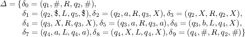
In $\varOmega _0$, $q_1$ is the initial state and $q_5$ is the acceptance state. Obviously, this LBA accepts the empty string. Figure 6 shows the constructed net corresponding to $\varOmega _0$ with the empty input string.

From Fig. 6 we can see that after firing transition $t_1$ at the initial marking $\{i\}$, transition $\langle 0,\delta _0\rangle$ can be fired if the tokens in $A_{0\#}$ and $B_{0,q_1}$ are allocated to the input places of transition $\langle 0,\delta _0\rangle$. After we fire $\langle 0,\delta _0\rangle$, if we allocate the tokens in $A_{1,\$}$ and $B_{1,q_2}$ to the input places of transition $\langle 1,\delta _1\rangle$, then $\langle 1,\delta _1\rangle$ is enabled and firing it leads to a marked $B_{q_5}$. At this time, $t_2$ and $t_3$ are both enabled; if the latter is chosen to fire, then a deadlock occurs; if the former is chosen to fire, then from any succeeding marking, marking $\{o\}$ is always reachable.

Fig. 6.

Safe ACWF-net corresponding to the LBA $\varOmega _0$ with the empty input string.

After firing transition $t_1$ at the initial marking $\{i\}$, none of transitions $\langle 0,\delta _0\rangle$, $\langle 0,\delta _9\rangle$ and $\langle 1,\delta _1\rangle$ can be fired if the token in symbol place $A_{0\#}$ is allocated to its image as an input place of transition $\langle 0,\delta _9\rangle$ and the token in state place $B_{0,q_1}$ is allocated to its image as an input place of transition $\langle 0,\delta _0\rangle$. At this time, either the state token is recycled to $v_8$ or transition $t_2$ is fired. Only after we fire $t_2$, the token in $v_8$ can be re-allocated to state places. Similarly, from any succeeding marking, marking $\{o\}$ is always reachable.

In a word, this safe ACWF-net is not sound.

3.3 PSPACE-completeness

Our construction contains at most

$$(\vert S\vert +2)(\vert Q\vert +\vert \varGamma \vert +2\vert \varDelta \vert +2)+13$$

places and at most

$$(\vert S\vert +2)(\vert Q\vert +\vert \varGamma \vert +5\vert \varDelta \vert )+10$$

transitions when we consider each tape cell corresponds to $\vert \varDelta \vert$ LBA transitions. For an LBA with an input string, therefore, we can construct a safe ACWF-net in polynomial time. From the above introduction, we can know that an LBA with an input string does not accept the string if and only if the constructed safe ACWF-net is sound. Therefore, we have the following conclusion:

Lemma 1

The soundness problem of safe ACWF-net is PSPACE-hard.

In order to prove the PSPACE-completeness, we should provide a PSPACE algorithm to decide soundness for safe ACWF-nets. In fact, we have provided such an algorithm when we proved that the soundness problem is PSPACE-complete for bounded WF-nets in [20]. It mainly utilised the PSPACE algorithm of deciding the reachability problem for bounded Petri nets provided in [8], and it is omitted here.

Theorem 1

The soundness problem of safe ACWF-net is PSPACE-complete.

Obviously, this conclusion can be extended to the soundness problem of bounded ACWF-nets since the PSPACE algorithm in [20] is applicable to any bounded WF-net.

Corollary 1

The soundness problem of bounded ACWF-net is PSPACE-complete.

Since the definition of soundness is a special case of the definition of weak soundness, we have the following conclusion:

Corollary 2

The weak soundness problem of bounded/safe ACWF-net is PSPACE-complete.

Aalst [2] proved that the soundness of a WF-net is equivalent to the liveness and boundedness of its short-circuit.

Proposition 1

([2]). Let $N =(P, T, F)$ be a WF-net and $\overline{N} =(P, T\cup \{t_0\},~F \cup \{(t_0,i), (o, t_0)\})$ be the short-circuit of N where $t_0\notin T$. Then, N is sound if and only if $(\overline{N}, \{i\})$ is live and bounded.

If we consider the short-circuit of our constructed ACWF-net for an LBA with an input string, we easily know that 1) this short-circuit is still asymmetric-choice and it is still safe at the initial marking $\{i\}$, and 2) it is live at the initial marking $\{i\}$ if and only if the LBA does not accept the input string. Therefore, based on Proposition 1 or our construction, we can draw the following conclusion:

Lemma 2

The liveness problem of safe AC-net is PSPACE-hard.

Cheng, Esparza and Palsberg [8] introduced a PSPACE algorithm⁴ to decide liveness of safe Petri nets, which is also applicable to safe AC-nets. Therefore, we have the following conclusion:

Theorem 2

The liveness problem of safe AC-net is PSPACE-complete.

Ohta and Tsuji [28] proved that the liveness problem of bounded AC-nets is NP-hard. Obviously, we sharpen their result.

We can know that the reachability problem for safe AC-nets is PSPACE-complete, which is based on the following facts: 1) the reachability problems for safe Petri nets and safe FC-nets are both PSPACE-complete [10], 2) safe AC-nets are a subclass of safe Petri nets, and 3) safe FC-nets are a subclass of safe AC-nets.

Theorem 3

The reachability problem of safe AC-net is PSPACE-complete.

4 Conclusion

In this paper, we first construct a safe FC-net to weakly simulate the computations of an LBA with an input string, and then add some controls into the FC-net so that the final net is a safe ACWF-net and the safe ACWF-net is sound if and only if the LBA does not accept the input string. We therefore prove that the soundness problem of safe ACWF-nets is PSPACE-hard, and this lower bound strengthens an existing result, i.e., NP-hardness provided in [18]. We have known that this problem is in PSPACE [20], and thus we obtain an accurate bound for this problem: PSPACE-complete. At the same time, we infer that the liveness problem of safe AC-nets is also PSPACE-complete. These results also provide a support to a rule of thumb proposed by Esparza in [12]: “All interesting questions about the behaviour of safe Petri nets are PSPACE-hard”.

From Table 1 we can see that there is a large gap between safe FC-nets and safe AC-nets (resp. safe FCWF-nets and safe ACWF-nets) about their liveness (resp. soundness) problem’s complexities: from polynomial-time to PSPACE-complete. These results also evidence that the computation power of AC-nets is much stronger than that of FC-nets. Although literatures [6, 7, 10, 31] provide many theorems that hold for FC-nets but fail for AC-nets, we still plan to explore some subclasses of AC-nets and ACWF-nets in future, motivated by the large gap and focusing on the following questions:

• 1. whether there is a subclass such that it is larger than safe FC-net (resp. safe FCWF-net) and smaller than safe AC-net (resp. safe ACWF-net), but its liveness (resp. soundness) problem is below PSPACE (e.g. NP-complete⁵)?

• 2. if there exists such a subclass, whether there is a good structure-based condition, just like that for FC-nets [6, 7, 10, 31], to decide their liveness and soundness?

References

van der Aalst, W.M.P.: Interorganizational Workflows: an approach based on message sequence charts and petri nets. Syst. Anal. Model. 34, 335–367 (1999)
van der Aalst, W.M.P.: Structural characterizations of sound workflow nets. Computing Science Report 96/23, Eindhoven University of Technology (1996)
van der Aalst, W.M.P., et al.: Soundness of workflow nets: classification, decidability, and analysis. Form. Aspects Comput. 23, 333–363 (2011). https://doi.org/10.1007/s00165-010-0161-4
van der Aalst, W., Kindler, E., Desel, J.: Beyond asymmetric choice: a note on some extensions. Petri Net Newsl. 55, 3–13 (1998)
Barkaoui, K., Pradat-Peyre, J.-F.: On liveness and controlled siphons in Petri nets. In: Billington, J., Reisig, W. (eds.) ICATPN 1996. LNCS, vol. 1091, pp. 57–72. Springer, Heidelberg (1996). https://doi.org/10.1007/3-540-61363-3_4
Best, E.: Structure theory of petri nets: the free choice hiatus. In: Brauer, W., Reisig, W., Rozenberg, G. (eds.) ACPN 1986. LNCS, vol. 254, pp. 168–205. Springer, Heidelberg (1987). https://doi.org/10.1007/978-3-540-47919-2_8
Best, E., Voss, K.: Free choice systems have home states. Acta Informatica 21, 89–100 (1984). https://doi.org/10.1007/BF00289141
Cheng, A., Esparza, J., Palsberg, J.: Complexity results for 1-safe nets. Theoret. Comput. Sci. 147, 117–136 (1995)
Czerwiński, W., Lasota, S., Lazić, R., Laroux, J., Mazowiecki, F.: The reachability problem for Petri nets is not elementary. In: Proceedings of the 51st Annual ACM SIGACT Symposium on Theory of Computing, pp. 24–33 (2019)
Desel, J., Esparza, J.: Free Choice Petri Nets. Cambridge Tracts in Theoretical Computer Science, vol. 40. Cambridge University Press, Cambridge (1995)
Esparza, J., Hoffmann, P., Saha, R.: Polynomial analysis algorithms for free choice probabilistic workflow nets. Perform. Eval. 117, 104–129 (2017)
Esparza, J.: Decidability and complexity of Petri net problems — an introduction. In: Reisig, W., Rozenberg, G. (eds.) ACPN 1996. LNCS, vol. 1491, pp. 374–428. Springer, Heidelberg (1998). https://doi.org/10.1007/3-540-65306-6_20
Garey, M.R., Johnson, D.S.: Computer and Intractability: A Guide to the Theory of NP-Completeness. W. H. Freeman and Company, New York (1976)
Hack, M.: Petri Net languages. Technical report 159, MIT (1976)
Jiao, L., Cheung, T.Y., Lu, W.: On liveness and boundedness of asymmetric choice nets. Theoret. Comput. Sci. 311, 165–197 (2004)
Jones, N.D., Landweber, L.H., Lien, Y.E.: Complexity of some problems in Petri nets. Theoret. Comput. Sci. 4, 277–299 (1977)
Leroux, J., Schmitz, S.: Reachability in vector addition systems is primitive-recursive in fixed dimension. In: Proceedings of the 34th Annual ACM/IEEE Symposium on Logic in Computer Science, pp. 1–13 (2019)
Liu, G., Jiang, C.: Co-NP-hardness of the soundness problem for asymmetric-choice workflow nets. IEEE Trans. Syst. Man Cybern.: Syst. 45, 1201–1204 (2015)
Liu, G., Jiang, C.: Net-structure-based conditions to decide compatibility and weak compatibility for a class of inter-organizational workflow nets. Sci. China Inf. Sci. 58, 1–16 (2015). https://doi.org/10.1007/s11432-014-5259-5
Liu, G., Sun, J., Liu, Y., Dong, J.: Complexity of the soundness problem of workflow nets. Fundamenta Informaticae 131, 81–101 (2014)
van Hee, K., Sidorova, N., Voorhoeve, M.: Generalised soundness of workflow nets is decidable. In: Cortadella, J., Reisig, W. (eds.) ICATPN 2004. LNCS, vol. 3099, pp. 197–215. Springer, Heidelberg (2004). https://doi.org/10.1007/978-3-540-27793-4_12
Kang, M.H., Park, J.S., Froscher, J.N.: Access control mechanisms for inter-organizational workflow. In: Proceedings of the Sixth ACM Symposium on Access Control Models and Technologies, pp. 66–74. ACM Press, New York (2001)
Kindler, E.: The ePNK: an extensible Petri net tool for PNML. In: Kristensen, L.M., Petrucci, L. (eds.) PETRI NETS 2011. LNCS, vol. 6709, pp. 318–327. Springer, Heidelberg (2011). https://doi.org/10.1007/978-3-642-21834-7_18
Kindler, E., Martens, A., Reisig, W.: Inter-operability of workflow applications: local criteria for global soundness. In: van der Aalst, W., Desel, J., Oberweis, A. (eds.) Business Process Management. LNCS, vol. 1806, pp. 235–253. Springer, Heidelberg (2000). https://doi.org/10.1007/3-540-45594-9_15
Malek, M., Ahmadon, M., Yamaguchi, S.: Computational complexity and polynomial time procedure of response property problem in workflow nets. IEICE Trans. Inf. Syst. E101–D, 1503–1510 (2018)
Martens, A.: On compatibility of web services. Petri Net Newsl. 65, 12–20 (2003)
Meyer, P.J., Esparza, J., Offtermatt, P.: Computing the expected execution time of probabilistic workflow nets. In: Vojnar, T., Zhang, L. (eds.) TACAS 2019. LNCS, vol. 11428, pp. 154–171. Springer, Cham (2019). https://doi.org/10.1007/978-3-030-17465-1_9
Ohta, A., Tsuji, K.: NP-hardness of liveness problem of bounded asymmetric choice net. IEICE Trans. Fundam. E85–A, 1071–1074 (2002)
Reisig, W.: Understanding Petri Nets: Modeling Techniques, Analysis Methods, Case Studies. Springer, Heidelberg (2013). https://doi.org/10.1007/978-3-642-33278-4
Tao, X.Y., Liu, G.J., Yang, B., Yan, C.G., Jiang, C.J.: Workflow nets with tables and their soundness. IEEE Trans. Ind. Inf. 16, 1503–1515 (2020)
Thiagarajan, P.S., Voss, K.: A fresh look at free choice nets. Inf. Control 61, 85–113 (1984)
Tiplea, F.L., Bocaenealae, C., Chirosecae, R.: On the complexity of deciding soundness of acyclic workflow nets. IEEE Trans. Syst. Man Cybern.: Syst. 45, 1292–1298 (2015)
Trčka, N., van der Aalst, W.M.P., Sidorova, N.: Data-flow anti-patterns: discovering data-flow errors in workflows. In: van Eck, P., Gordijn, J., Wieringa, R. (eds.) CAiSE 2009. LNCS, vol. 5565, pp. 425–439. Springer, Heidelberg (2009). https://doi.org/10.1007/978-3-642-02144-2_34
Verbeek, H.M.W., van der Aalst, W.M.P., Ter Hofstede, A.H.M.: Verifying workflows with cancellation regions and OR-joins: an approach based on relaxed soundness and invariants. Comput. J. 50, 294–314 (2007)
Wimmel, H.: Synthesis of reduced asymmetric choice Petri nets. arXiv:1911.09133, pp. 1–27 (2019)
Xiang, D.M., Liu, G.J., Yan, C.G., Jiang, C.J.: A guard-driven analysis approach of workflow net with data. IEEE Trans. Serv. Comput. (2019, published online). https://doi.org/10.1109/TSC.2019.2899086
Yamaguchi, S., Matsuo, H., Ge, Q.W., Tanaka, M.: WF-net based modeling and soundness verification of interworkflows. IEICE Trans. Fundam. Electron. Commun. Comput. Sci. E90–A, 829–835 (2007)
van Zelst, S.J., van Dongen, B.F., van der Aalst, W.M.P., Verbeek, H.M.W.: Discovering workflow nets using integer linear programming. Computing 100(5), 529–556 (2017). https://doi.org/10.1007/s00607-017-0582-5
Acknowledgement
The author would like to thank the anonymous reviewers for their very detailed and constructive comments that help the author improve the quality of this paper. This paper was supported in part by the National Key Research and Development Program of China (grant no. 2018YFB2100801), in part by the Fundamental Research Funds for the Central Universities of China (grant no. 22120190198) and in part by the Shanghai Shuguang Program (grant no. 15SG18).
Author information
Authors and Affiliations
Corresponding author
Editor information
Editors and Affiliations
Rights and permissions
Copyright information
© 2020 Springer Nature Switzerland AG
About this paper
Cite this paper
Liu, G. (2020). PSPACE-Completeness of the Soundness Problem of Safe Asymmetric-Choice Workflow Nets. In: Janicki, R., Sidorova, N., Chatain, T. (eds) Application and Theory of Petri Nets and Concurrency. PETRI NETS 2020. Lecture Notes in Computer Science(), vol 12152. Springer, Cham. https://doi.org/10.1007/978-3-030-51831-8_10
Download citation
DOI: https://doi.org/10.1007/978-3-030-51831-8_10
Published:
Publisher Name: Springer, Cham
Print ISBN: 978-3-030-51830-1
Online ISBN: 978-3-030-51831-8
eBook Packages: Computer ScienceComputer Science (R0)