AI for Localizing Faults in Spreadsheets

Abstract

Localizing faults in programs is considered a demanding task. A lot of effort is usually spent in finding the root cause of a misbehavior and correcting the program such that it fulfills its intended behavior. The situation is even worse in case of end user programming like spreadsheet development where more or less complex spreadsheets are developed only with little knowledge in programming and also testing. In order to increase quality of spreadsheets and also efficiency of spreadsheet development, tools for testing and debugging support are highly required. In this paper, we focus on the latter and show that approaches originating from Artificial Intelligence can be adapted for (semi-) automated fault localization in spreadsheets in an interactive manner. In particular, we introduce abstract models that can be automatically obtained from spreadsheets enabling the computation of diagnoses within a fraction of a second. Besides the basic foundations, we discuss empirical results using artificial and real-world spreadsheet examples. Furthermore, we show that the abstract models have a similar accuracy to models of spreadsheets capturing their semantics.

1 Introduction

Quality assurance of software and systems is an important part of development to avoid failures occurring after deployment. Activities like testing at all levels are part of all currently used development processes where experienced and educated personnel is involved. This unfortunately does not hold in spreadsheet programming where end users are developing programs, who are usually not educated in program development. In addition, in spreadsheet development it is not easy to distinguish testing from programming, and further more, the programs themselves, i.e., the equations assigned to cells, are not that visible during development. As a consequence, there is a 3–5% error rate when writing formulae in spreadsheets (see Panko [16]). Therefore, there is a need for tools supporting testing and fault localization during spreadsheet development specifically considering the end-user aspect, requiring tools that easily and transparently integrate into spreadsheet development causing a high degree of interactivity. Previously developed approaches to spreadsheet fault localization like [7] are not sufficient due to high runtime requirements. There Hofer and colleagues reported that computing single faults including repair suggestions took 25.1 s even for smaller spreadsheets having up to 70 non-empty cells.

In this paper, we focus solely on spreadsheet fault localization aiming at improving runtime whereas not reducing the quality of diagnosis. For this purpose, we introduce abstract models that can be automatically derived from spreadsheets and used for (semi-)automated fault localization. In order to show how models can be used for fault localization, let us have a look at a small example. In Fig. 1(a) we see a spreadsheet allowing to compute payments of Mr. Green and Mrs. Jones based on their weekly working hours and their hourly rate. In Fig. 1(b) we have the same spreadsheet but with a fault in cell D2 introduced. What we immediately see is that the values of cells F2 and D4 are lower than expected. Note that in practice at least the failure in cell F2 would have been easily detected because Mr. Green would complain about the lower payment to be received for two weeks. When having a look at the equations stored (see Fig. 1(c)), the reason behind the failures becomes obvious. Instead of summing up the hours of week 1 and week 2 in cell D2 only the working hours for week 1 are considered. But how to find such a bug using the available information?

Fig. 1.

A small spreadsheet example (a variant from the EUSES corpus [5])

In the following, we make use of the equations stored in the spreadsheets, their references to other cells and assumptions about the correctness of cells to localize the faulty cell. Let us, for example, assume that all cells except cell D2 are correct. In practice, we obtain this information from the spreadsheet user, who indicates his/her observations about the computed values. Additionally, we make use of the expected values for cells F2 and D4, which are 810 and 123 respectively. From the values of E2 and the expected value of F2 we can derive a value of 54 for cell D2 (Note, 54 = 810/15). When using this value and the value of cell D3 we finally receive 123 (=54 + 69), which is exactly the expected value for cell D4. Hence, D2 is a potential root cause, but are there more? We can use the same idea but in this case we assume all cells except cell F2 to be correct. In this case, we would get again a value of 92 for cell D4 when using the underlying equations. Therefore, cell F2 alone is not a candidate. When assuming F2 and D4 to be faulty, we would not be able to compute values for cells F2 and D4 and there is no contradiction when comparing these values with the expected ones. Hence, we have another root cause comprising cells F2 and D4. In most cases we are more interested in smaller explanations. In this case, we would prefer diagnosis D2 over diagnosis F2, D4.

What can we take from this brief example? First, we only considered the available equations for computing values. Second, we used assumptions about the correctness of cells. In case a cell is assumed to be correct, we used the corresponding equation. Otherwise, we ignored the equation and did not compute any value using this equation. Computing all diagnoses can be simplified done assuming all subsets of cells comprising equations to be faulty and the others to be correct, and checking whether the computable values are contradicting input values or expected output values. Unfortunately, this is computationally infeasible. In addition, equation solving is also computationally demanding, and there is a need for abstract models. An abstract model, for example, might only consider information regarding whether a certain value is smaller, equivalent, or larger than expected, or whether the value is correct or not correct. In our running example, we obtain that the value of cells F2 and D4 are both too small. When assuming cell F2 to work as expected and assuming that the cells comprising only values are correct (like done previously), we can immediately conclude that also the value of cell D2 is too small. With similar arguments than before when using the equations and real values, we are able to come up with similar diagnoses. We will discuss the abstract models in detail in the next section. The idea behind abstract models dealing with qualities instead of quantitative values comes from Qualitative Reasoning (QR), which is a subfield of Artificial Intelligence (AI).

The consequences when using abstract models instead of the stored equations and values are interesting. Do we compute more diagnoses? Do the computed diagnoses always include the real fault? What is the impact of abstract models on the runtime? And finally, are there any other consequences when using real world spreadsheets? In this paper, we will discuss these questions and also give answers. In summary, the contributions of this paper are:

• Providing a solid foundation for model-based debugging of spreadsheets, which is based on previous work on model-based diagnosis [17, 19].

• Introducing three different types of models where one makes use of a qualitative representation of deviations between the expected and the current spreadsheet.

• Comparing the different types of models with respect to their diagnosis accuracy and runtime.

The paper is organized as follows. First, we introduce the basic definitions of diagnosis and discuss the underlying models. Afterwards, we present the results of our experimental evaluation, where we focus on the runtime issue and the diagnosis accuracy. Finally, we conclude the paper, which includes a brief discussion on related research.

2 Basic Definitions

Wotawa [19] described the use of constraints for fault localization. Constraints are basically equations or conditions on variables that must hold in order to be satisfied. For example, the constraint $x = 2 \cdot y$ is satisfied when assigning a value of 2 to variable x and 1 to variable y. When given a set of constraints the aim of constraint solving is to provide variable assignments such that all constraints are satisfied. For a deeper introduction into constraint solving including algorithms we refer the interested reader to Dechter [4]. However, in order to be self-contained, we briefly introduce the basic concepts of constraint solving first, discuss automated diagnosis afterwards, and show how spreadsheets can be compiled into three different constraint representations for the purpose of automated fault localization.

Constraint Solving: We define a constraint system as a tuple $(\textit{VARS},\textit{DOM},$ $\textit{CONS})$ where $\textit{VARS}$ is defined as a finite set of variables, $\textit{DOM}$ is a function mapping each variable to its domain comprising at least one element, and $\textit{CONS}$ is a finite set of constraints. Without restricting generality we define a constraint c as a pair $((v_1,\ldots ,v_k),tl)$ where $(v_1,\ldots ,v_k)$ is a tuple of variables from $\textit{VARS}$, and tl a set of tuples $(x_1,\ldots ,x_k)$ of values where for each $i\in \{1,\ldots ,k\}$: $x_i \in \textit{DOM}(v_i)$. The set of tuples tl in this definition declares all allowed variable value combinations for a particular constraint. For simplicity, we assume a function $\textit{scope}(c)$ for a constraint c returning the tuple $(v_1,\ldots ,v_k)$, and a similar function tl(c) returning the set of tuples tl of c.

Searching for solutions of given constraint systems is equivalent to searching for values assigned to all variables such that all constraints are satisfied. The corresponding problem is called constraint satisfaction problem (CSP). In order to formally define CSP we first start defining value assignments: Given a constraint system $(\textit{VARS}, \textit{DOM}, \textit{CONS})$, and variable $v \in \textit{VARS}$, then $v = x$ with $x \in \textit{DOM}(v)$ is a single assignment of a value x to the variable v. We further define a value assignment as a set of single assignments where there is at maximum one single assignment for each variable. A constraint c with scope $(v_1,\ldots ,v_k)$ fulfills a value assignment $\{\ldots , v_1 = x_1, \ldots , v_k = x_k, \ldots \}$, if there exists a tuple $(x_1,\ldots ,x_k)$ in the constraint tl(c). Otherwise, we say that such a value assignment contradicts the constraint.

Example 1

Cell D3 of the spreadsheet in Fig. 1(c) contains the formula $\text{ B3 } + \text{ C3 }$. We model this by using the constraint $((B3, C3, D3),\{(a,b,a + b) | a,b \in \mathbb {N}\})$ where B3, C3, D3 are the variables representing the value of cells B3, C3, D3 respectively.

Using the definition of value assignments, we are now able to define CSPs. A CSP for a given constraint system is defined as question whether there exists a value assignment that fulfills all given constraints. If there is such a value assignment, the CSP is said to be fulfilled. Solving a constraint satisfaction problem is computationally demanding but there are efficient algorithms available, e.g. [6].

Model-Based Diagnosis: Model-based diagnosis is an AI method for computing all diagnoses from an available model of a system or in our case spreadsheet. The underlying idea is to make the assumptions about correctness of a component explicit. For each component, we add a model representing its behavior. Diagnosis becomes searching for assumptions about the correctness of certain components of a system: Which components are correct and which behave faulty so that given observations are not in contradiction with values obtained using the model?

Reiter [17] defines a diagnosis problem as a tuple $(\textit{COMP}, \textit{SD}, \textit{OBS})$ where $\textit{COMP}$ is a set of components, $\textit{SD}$ a logical sentence describing the behavior of the system, i.e., the system description, and $\textit{OBS}$ a set of observations. In our case, the observations are the information we obtain from the user who indicates that a certain cell contains a wrong value while others compute the correct result. When using constraints for diagnosis, we have to slightly modify this definition. We assume a constraint representation of the system and additional constraints specifying the observations. In this context, the diagnosis problem becomes a tuple $(\textit{VARS}, \textit{DOM}, \textit{CONS}\, \cup \textit{COBS})$ where $(\textit{VARS},\textit{DOM},\textit{CONS})$ is a constraint representation of a system comprising variables $ab_C$ for every component C of the system, and $\textit{COBS}$ is the constraint representation of all observations $\textit{OBS}$.

Example 2

(Continuation of Example 1 ). Assuming that the values of B3 and C3 are correct, then D3 either computes the desired output or its formula is faulty. We can model this by using the following constraint where we introduced a variable $ab_{D3}$ representing the assumption that cell D3 is faulty:

$$((ab_{D3}, B3, C3, D3),\{(F,a,b,a + b) | a,b \in \mathbb {N}\} \cup \{(T,a,b,c)| a,b,c \in \mathbb {N}\}).$$

We can create such constraints for all formula cells to represent the spreadsheet given in Fig. 1. For simplicity, in the following model, we only consider the cells D2, D3, and D4. The constraints for D2, D4 are similar to the one of D3. This set of constraints builds the system description $\textit{SD}$. The given formula cells build the set of components $\textit{COMP}$, i.e. $\textit{COMP}=\{D2,D3,D4\}$. The set of observations contains the information about the correct and erroneous output as well as the input cells and their values: $\textit{OBS}=\{B2=23, C2=31, B3=35, C3=34, D4=123\}$. The observations can be easily represented as a constraint, e.g., $((B2,B3,C2,C3,D4), \{(23,35,31,34,123)\})$.

Given a diagnosis problem a solution, i.e., a diagnosis, is a subset of the set of components $\textit{COMP}$ so that assuming all components in a diagnosis to be faulty, allows to compute a solution for the corresponding constraint representation. Formally, a diagnosis $\varDelta \subseteq COMP$ is a diagnosis if and only if the following constraint system is satisfiable, i.e., there exists a solution for: $\textit{CONS}\, \cup \textit{COBS}\, \cup \{ ((ab_C), \{ (T) | C \in \varDelta \}), ((ab_C), \{(F) | C \in \textit{COMP} \setminus \varDelta \})\}$. There could be more than one diagnosis. We are usually focusing on minimal diagnoses only. A minimal diagnosis in our setting is a diagnosis where none of its subsets is itself a diagnosis.

Nica and Wotawa [15] introduced the ConDiag algorithm that allows computing all minimal diagnoses up to a predefined size using the constraint representation of a diagnosis problem. Algorithm 1 illustrates the pseudo-code of ConDiag. At the beginning of the algorithm, the result and the model are initialized (line 1–2). Within the loop the constraint model is constructed (line 4) bringing together the initial model M and the assumption that we are only interested in diagnoses of size i. Afterwards, in line 5 the constraint solver is called returning all diagnoses of size i. If the constraint system is satisfiable for i = 0, we terminate ConDiag and return the set comprising the empty set as results meaning that the system is fault free. In line 9 the new diagnoses are added and in line 10 a new constraint is added to the model. This constraint basically states that we are not interested in supersets of already computed diagnoses. The loop continues until we reach the maximum size. ConDiag always terminates (providing the constraint solver terminates) and computes all minimal diagnoses up to a pre-defined size n. ConDiag is also efficient. Nica et al. [14] compared ConDiag with other diagnosis algorithms showing a good overall runtime. In practice, n is usually set to 1 up to 3.

Modeling for Spreadsheets: For making use of model-based diagnosis for spreadsheet fault localization, we have to provide a constraint model of the spreadsheet. For simplicity, we assume a spreadsheet to be a finite set of cells $\{c_1,\ldots ,c_k\}$. Each cell $c_i$ is uniquely identifiable using its row and column. Like in ordinary spreadsheet implementations we write a cell as Ar where A denotes the column using letters, and r the row using natural numbers. A cell c has a value and maybe a corresponding formula. In case c has attached a formula its value is determined by the formula. Without restricting generality, we assume every formula to be of the form $c_1~ op~ c_2$ where $c_1$, $c_2$ are (references to) cells and op is an operator $+,-,/$, or $*$. A cell with no formula attached is called an input cell. A cell that is never referenced in a formula is called an output cell.

Algorithm 2 gives the pseudo-code of a compiler that takes a spreadsheet as input and computes its corresponding constraint representation. The algorithm Compile2Model makes use of two functions $\textit{constraint}_F$ and $\textit{constraint}_O$ which compute the constraint representation of formulae and observations respectively. These functions depend on the used model type: We explain the functions for the three different types of models in this paper. One model directly represents the behavior of formulae (called value-based model) and serves as reference model. The other model (called dependency-based model) only considers knowledge about the correctness of values, whereas the third model (called comparison-based model) uses the deviations of cell values. The last two models are abstract models not considering the real values used in spreadsheets.

In line 3, all cells of the spreadsheet are added to the set of variables VAR and are assigned an domain DOM depending on the underlying model: $\textit{DOM}=\mathbb N$ when using the value-based model, $\textit{DOM}=\mathbb B$ when using the dependency-based model, and $\textit{DOM}=\{0,1,2\}$ when using the comparison-based model. For all cells containing equations, an additional variable $ab_c$ is added to VAR with $\textit{DOM}(ab_c)=\mathbb B$ and the equations are translated into constraints (lines 4–7). Finally, the constraints for the observations are added using the function $\textit{constraint}_O$. The functions $\textit{constraint}_F$ and $\textit{constraint}_O$ for the different models are defined as follows:

• Value-based model (VM): The VM directly represents spreadsheets. Formulae are directly represented as constraints. Let us assume a formula $c_1 ~op~ c_2$ stored in cell c. The function $constraint_F(c)$ returns the constraint $((ab_c, c_1,c_2,c),\{(F,a,b,a~op~b) | a,b \in \mathbb N\} \cup \{(T,a,b,c) | a,b,c \in \mathbb N\}).$

  In this constraint, we distinguish the correct case where $ab_c$ is set to false from the faulty case. In the latter case, there are no restrictions on the values of cells c, $c_1$, $c_2$. For the representation of observations, we assume to have a set $\{c_1=v_1,\ldots ,c_k=v_k\}$. In this case $constraint_O$ returns one constraint $((c_1,\ldots ,c_k),\{(v_1,\ldots ,v_k)\})$.

• Dependency-based model (DM): The DM only considers values being correct or not correct, which are represented using the numbers 1 and 0 respectively. A formula $c_1 ~op~ c_2$ for a cell c cannot be directly represented as constraint. Instead, we make use of the following idea: A formula returns a definitely correct value only if both input values are correct. In cases where we do not have fault masking, we are also able to say that a correct value computed using a formula also requires both inputs to be correct. This assumption is not always true. However, in case of using only numbers failure masking has a very low probability. More information on this improved version of the dependency-based model can be found in [8, 10].

  Taking the idea of dealing with correctness and incorrectness of values, we are able to define $constraint_F$ as a function returning the constraint $((ab_c, c_1,c_2,c), T_D)$ where $T_D$ is a set comprising the following elements:

  $$\begin{array}{rrrr} \hline ab_{XY} &{} c_1 &{} c_2 &{} c \\ \hline F &{} 1 &{} 1 &{} 1 \\ F &{} 0 &{} 1 &{} 0 \\ F &{} 1 &{} 0 &{} 0 \\ F &{} 0 &{} 0 &{} 0 \\ \hline T &{} . &{} . &{} . \\ \hline \end{array}$$

  In this table “.” stands for arbitrary values. Thus, in case of a fault all possible combinations are considered. For the observations, we define $\textit{constraint}_O$ as follows: Let us assume to have a set $\{c_1=v_1,\ldots ,c_k=v_k\}$ and a function $\delta$ with the cell and its value as parameters. $\delta (c,v)$ returns 1 if c is an input cell or if the value of cell c provided when executing the spreadsheet is equivalent to v. Otherwise, $\delta$ returns 0. $\textit{constraint}_O$ returns a constraint of the following form: $((c_1,\ldots ,c_k),\{(\delta (c_1,v_1),\ldots ,\delta (c_k,v_k))\})$.

• Comparison-based model (CM): CM is very similar to DM. But instead of only considering values to be correct or incorrect, we consider values to be smaller, equivalent or larger than expected represented using the numbers 0, 1, and 2 respectively. The function $constraint_E$ applied to formula $c_1~op~ c_2$ of cell c returns a constraint $((ab_c, c_1,c_2,c), T_D)$ where $T_D$ is a set comprising elements depending on the underlying operator. The table for operators + and * is given on the right; the table for operators − and / is given on the left:

  

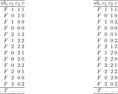
  Again, “.” stands for arbitrary values and in case of a fault we consider all possible combinations to be part of the constraint values. For the observations and function $constraint_O$, we make use of a similar idea than for DM. Instead of using function $\delta$, we define a function $\psi$ with the cell and its value as parameters. $\psi (c,v)$ returns 0 if c is not an input cell and the value computed when executing the spreadsheet is smaller than v. $\psi$ returns 1 if c is an input cell or if the value of cell c provided when executing the spreadsheet is equivalent to v. Otherwise, $\psi$ returns 2. Function $constraint_O$ returns a constraint of the following form: $((c_1,\ldots ,c_k),\{(\psi (c_1,v_1),\ldots ,\psi (c_k,v_k))\})$.

3 Experimental Evaluation

In this section, we present and discuss empirical results obtained using a class of artificially generated examples and real-world spreadsheets. The purpose of this section is to answer the questions whether the comparison-based model has a good runtime and accuracy compared with the dependency-based model and the value-based model. The latter can be seen as reference model because it is more or less a one-to-one representation of its corresponding spreadsheet. For solving the constraints, we used Minion [6], an out-of-the-box, open source constraint solver that supports arithmetic, relational, and logic constraints over Boolean and Integers.

In the first part of the experimental evaluation, we focused mainly on the question regarding the runtime of the different models to compute all diagnoses. Therefore, we used a parametrizable example comprising components for adding and multiplying integers, which is close to an ordinary spreadsheet for calculating sums of numbers. For the artificial example have a look at Fig. 2 where we have parameters $m, n \ge 2$. From the figure we see that we obtain $((n+4)\cdot m) - 3$ components for given parameters in total. For the experiment, we implemented an input-output values generator, which randomly assigns values to the $m \times n$ inputs $x_{i~j}$ and computes the expected m outputs $z_k$, and outputs $y_1, y_2, y_3$. Furthermore, we implemented a model generator, which returns the three models and the observations directly as constraints.

Fig. 2.

Parametrizable example with $m \times n$ inputs $x_{i~j}$, m outputs $z_k$, and outputs $y_1$, $y_2,$ and $y_3$.

In Table 1, we summarize the obtained results when running the search for single, double, and triple diagnoses on a Windows 10 Pro notebook with a Intel(R) Core(TM) i7-4500U CPU 1.80 GHz and 8 GB of RAM. For the dependency-based and comparison-based model, we carried out ten runs and give the obtained average values in the table. For the value-based model, we used only three runs due to the very high runtime requirements, especially when carrying out the computation of triple fault diagnoses. The times given in Table 1 are in milli-seconds. The table has two parts. In the upper one, the results when setting only one output to a wrong value are given. The lower part comprises the results obtained when introducing failures at two outputs.

Table 1. Results for parametrizable example with V representing the value-based model, C representing the comparison-based model and D representing the improved dependency-based model. Note that Minion is called with -timelimit 1200

From Table 1 we see that in case of one output to be faulty the dependency-based and the comparison-based models provide the same set of diagnoses that is substantially different from the results obtained using the value-based model. In contrast, the more abstract models are less computationally demanding. In case of two output values that are different to the expected value, the situation is different. Here, the comparison-based model provide less diagnoses than the dependency-based model. The runtime again is much better for the more abstract models. Figure 3 shows the runtime of diagnosis using all three models as a function of the number of components. The dependency-based and the comparison-based model provide a similar runtime behavior whereas the value-based model requires a lot more time for computing all single fault diagnoses. This hold for the case of single failures as well as for double failures.

Fig. 3.

Runtime using parametrizable example for computing all single fault diagnoses

In the second part of the empirical evaluation, we used a subset of the publicly available Integer spreadsheet corpus [3]¹. This corpus contains spreadsheets with up to three artificially seeded faults. Unfortunately, we have to exclude some of the spreadsheets from our evaluation for two reasons: First, Minion was not able to compute any solutions at all within a time limit of 20 min for some of the spreadsheets when using the value-based model. Second, our prototype does not support the conversion of IF and MAX expressions to constraints. This is not a limitation of the approach, but only a limitation of the prototype. We have used an Intel Core processor (2.90 GHz) with 8 GB RAM, a 64-bit version of Windows 8 and MINION version 1.8 for this part of the evaluation.

Table 2 shows the results for 35 faulty spreadsheets. The spreadsheets are categorized into three groups: 15 spreadsheets whose true fault is a single fault, 14 spreadsheets with a double fault as true fault and 6 spreadsheets with a triple fault as true fault. The runtime is the time Minion requires to parse and solve the given constraint system for the indicated diagnosis size (1, 2, 3). The indicated times are the arithmetic mean over 10 runs. Whenever we have indicated ‘0’ as time, Minion required less than 0.5 ms and therefore returned 0 ms as solving time. Whenever we have indicted ‘-’ as time, Minion’s solving process exceeded a time limit of 20 min. The value-based model requires significantly more time than the dependency-based and comparison-based model and Minion could not compute double (respectively triple) fault diagnoses for 6 (respectively 7) spreadsheets. The reason for the poor runtime behavior of the value-based model lies in the different domain sizes: The abstract models restrict the variables’ domains to a size of 2 (dependency-based model) respectively 3 (comparison-based model); the value-based model reasons of Integer values ranging from $-2,000$ to 50,000. The comparison-based model and the dependency-based model have similar runtimes.

Table 2. Results for Integer Corpus with V representing the value-based model, C representing the comparison-based model and D representing the improved dependency-based model. The solving time and the number of diagnoses are separately indicated for single (1), double (2), and triple (3) fault diagnoses. An ‘-’ entry indicates a timeout. The entries of the columns ‘Faults founds’ indicate whether the model has the true fault as one of its diagnoes (Y) or only a subset of it (P). ‘Obs.’ provides information about the observations, where column ‘F’ indicates the number of observations where the computed output contradicts the expected output and ‘T’ indicates those where the computed output is equal to the expected one.

The value-based model performs better than the abstract models w.r.t. their diagnostic accuracy. For 22 spreadsheets, all models compute the same single fault diagnoses. For 13 spreadsheets, value-based model computed fewer diagnoses while the abstract models have the same single fault diagnoses. For two spreadsheets, the comparison-based model computed fewer single fault diagnoses than the value-based model.

An important question is whether the models are able to detect the true fault. This information is given in Table 2 in the columns labeled ‘Fault found’. An ‘Y’ entry indicates that the fault was reported as diagnosis; a ‘P’ entry indicates that only a part of the true fault (i.e. a subset) was reported as diagnosis, e.g. {D4} was reported as diagnosis, but {D4, D5} is the true fault. This is no problem per se, because all supersets of a diagnosis are also considered as diagnoses. However, the exacter a diagnosis is, the more helpful it is for spreadsheet programmers. For all spreadsheets with a single fault as true fault, the true fault has been reported as diagnosis. For two of the spreadsheets with a double fault, the value-based and the comparison-based models identified the true fault as one of the diagnoses, while the dependency-based model detected a subset as diagnosis. For all other spreadsheets with double faults, all models reported subsets of the true fault as diagnosis. All models identified the true diagnosis only for one of the triple fault spreadsheets, while they identified a subset of the true fault as diagnosis for all other triple fault spreadsheets.

The columns ‘Obs.’ provide information about the observations used. The ‘F’-column indicates the number of non-input observations where the computed value differs from the expected value; the ‘T’-column indicates the number of non-input observations where the computed value is equal to the expected value.

To summarize, the second part of the empirical evaluation shows that model-based diagnosis can be used to debug artificially created and real-life spreadsheets when an abstract model is used. Unfortunately, the value-based model requires too much runtime and therefore cannot be used in practice. The comparison-based and the dependency-based models convince by their low computation times of several milliseconds. These low computation times allow us to use these models in real-life scenarios, where a user expects to obtain the diagnosis candidates immediately after starting the diagnosis process. When comparing the diagnostic accuracy, the abstract models nearly reach the results of the value-based model. In practice, the slightly worse diagnostic accuracy is a good tradeoff for the runtime performance gain.

4 Conclusions

Using models for localizing faults in spreadsheets is not novel. Jannach and Engler [11] introduced the use of constraint solving for spreadsheet debugging for the first time. Later the same authors presented an add-on for Excel, the EXQUISITE debugging tool [12]. Abreu et al. [2] presented a similar approach. In contrast to Jannach and Schmitz’s approach, this approach relies on a single test case, and directly encodes the reasoning about the correctness of cells into the CSP. Hofer et al. [8, 10] were the first proposing to use dependency-based models for spreadsheet debugging. In contrast to this work, we – in addition – introduce a general framework for obtaining different models, discuss the comparison-based model, and present a detailed empirical evaluation comparing the different models. Other approaches to fault localization not based on model-based reasoning include Ruthruff et al. [18], Hofer et al. [9], and Abraham and Erwig [1]. For more details about quality assurance methods, we refer the interested reader to Jannach et al.’s survey paper [13], which provides an exhaustive overview on different techniques and methods for detecting, localizing, and repairing spreadsheets.

In this paper, we introduce a framework for fault localization based on models. In particular, we presented the underlying foundations and introduced an algorithm that allows compiling spreadsheets directly into models represented as set of constraints. Furthermore, we discussed three different types of models. The value-based model directly represents the behavior of a spreadsheet. The comparison-based model makes use of deviations between correct cell values and the actual values. The dependency-based model only distinguishes faulty from correct values occurring during computation. In addition, to the foundations and models, we presented empirical results obtained using generated examples that are parametrizable, and real-world spreadsheet programs comprising faults. The parametrizable spreadsheet has a structure and behavior close to spreadsheets occurring in practice. With the empirical evaluation we wanted to get answers to the following two questions: (1) Which model provides a good runtime performance? And, (2) whether the comparison-based model provides a good diagnosis accuracy?

From the obtained runtime results we can conclude that the dependency-based and the comparison-based model provide a good runtime performance and provide diagnoses much faster than the value-based model. With the dependency-based and the comparison-based model we are able to provide diagnosis capabilities almost at real time. Regarding diagnosis accuracy, the dependency-based and the comparison-based model are both weaker than the value-based model, which served as reference model in this case. The comparison-based model provides in some but not all cases a better diagnosis accuracy compared to the dependency-based model. This holds especially in cases where more than 1 output can be classified as faulty. Because of a similar runtime performance and a slightly better diagnosis accuracy the comparison-based model can be considered as superior to the dependency-based model.

References

Abraham, R., Erwig, M.: GoalDebug: a spreadsheet debugger for end users. In: 29th International Conference on Software Engineering (ICSE), pp. 251–260 (2007)
Abreu, R., Hofer, B., Perez, A., Wotawa, F.: Using constraints to diagnose faulty spreadsheets. Softw. Qual. J. 23(2), 297–322 (2015)
Ausserlechner, S., Fruhmann, S., Wieser, W., Hofer, B., Spork, R., Muhlbacher, C., Wotawa, F.: The right choice matters! SMT solving substantially improves model-based debugging of spreadsheets. In: 13th International Conference on Quality Software, pp. 139–148 (2013)
Dechter, R.: Constraint Processing. Morgan Kaufmann, San Francisco (2003)
Fisher, M.I., Rothermel, G.: The EUSES spreadsheet corpus: a shared resource for supporting experimentation with spreadsheet dependability mechanisms. ACM SIGSOFT Softw. Eng. Notes 30(4), 1–5 (2005)
Gent, I.P., Jefferson, C., Miguel, I.: Minion: a fast, scalable, constraint solver. In: Proceedings of the 17th European Conference on Artificial Intelligence (ECAI 2006) (2006)
Abreu, R., Außerlechner, S., Hofer, B., Wotawa, F.: Testing for distinguishing repair candidates in spreadsheets – the mussco approach. In: El-Fakih, K., Barlas, G., Yevtushenko, N. (eds.) ICTSS 2015. LNCS, vol. 9447, pp. 124–140. Springer, Cham (2015). doi:10.1007/978-3-319-25945-1_8
Hofer, B., Hoefler, A., Wotawa, F.: Combining models for improved fault localization in spreadsheets. IEEE Trans. Reliab. 66(1), 38–53 (2017)
Hofer, B., Perez, A., Abreu, R., Wotawa, F.: On the empirical evaluation of similarity coefficients for spreadsheets fault localization. Autom. Softw. Eng. 22(1), 47–74 (2015)
Hofer, B., Wotawa, F.: Why does my spreadsheet compute wrong values? In: Proceedings of the International Symposium on Software Reliability Engineering (ISSRE), vol. 25, pp. 112–121 (2014)
Jannach, D., Engler, U.: Toward model-based debugging of spreadsheet programs. In: 9th Joint Conference on Knowledge-Based Software Engineering (JCKBSE 2010), pp. 252–264 (2010)
Jannach, D., Schmitz, T.: Model-based diagnosis of spreadsheet programs - a constraint-based debugging approach. Autom. Softw. Eng. 23(1), 105–144 (2016). Springer
Jannach, D., Schmitz, T., Hofer, B., Wotawa, F.: Avoiding, finding and fixing spreadsheet errors - a survey of automated approaches for spreadsheet QA. J. Syst. Softw. 94, 129–150 (2014)
Nica, I., Pill, I., Quaritsch, T., Wotawa, F.: A route to success - a performance comparison of diagnosis algorithms. In: Proceedings of the International Joint Conference on Artificial Intelligence (IJCAI) (2013)
Nica, I., Wotawa, F.: Condiag - computing minimal diagnoses using a constraint solver. In: Proceedings of the International Workshop on Principles of Diagnosis (DX), pp. 185–191 (2012)
Panko, R.R.: Thinking is bad: implications of human error research for spreadsheet research and practice. In: CoRR (2008)
Reiter, R.: A theory of diagnosis from first principles. Artif. Intell. 32(1), 57–95 (1987)
Ruthruff, J., Creswick, E., Burnett, M., Cook, C., Prabhakararao, S., Fisher II, M., Main, M.: End-user software visualizations for fault localization. In: Proceedings of the 2003 ACM Symposium on Software Visualization (SoftVis 2003), pp. 123–132. ACM (2003)
Wotawa, F.: On the use of qualitative deviation models for diagnosis. In: 29th International Workshop on Qualitative Reasoning (QR), New York, July 2016
Acknowledgments
The work described in this paper has been funded by the Austrian Science Fund (FWF) project DEbugging Of Spreadsheet programs (DEOS) under contract number I2144 and the Deutsche Forschungsgemeinschaft (DFG) under contract number JA 2095/4-1.
Author information
Authors and Affiliations
Corresponding author
Editor information
Editors and Affiliations
Rights and permissions
Copyright information
© 2017 IFIP International Federation for Information Processing
About this paper
Cite this paper
Hofer, B., Nica, I., Wotawa, F. (2017). AI for Localizing Faults in Spreadsheets. In: Yevtushenko, N., Cavalli, A., Yenigün, H. (eds) Testing Software and Systems. ICTSS 2017. Lecture Notes in Computer Science(), vol 10533. Springer, Cham. https://doi.org/10.1007/978-3-319-67549-7_5
Download citation
DOI: https://doi.org/10.1007/978-3-319-67549-7_5
Published:
Publisher Name: Springer, Cham
Print ISBN: 978-3-319-67548-0
Online ISBN: 978-3-319-67549-7
eBook Packages: Computer ScienceComputer Science (R0)