Partitioning via Non-linear Polynomial Functions: More Compact IBEs from Ideal Lattices and Bilinear Maps

Abstract

In this paper, we present new adaptively secure identity-based encryption (IBE) schemes. One of the distinguishing properties of the schemes is that it achieves shorter public parameters than previous schemes. Both of our schemes follow the general framework presented in the recent IBE scheme of Yamada (Eurocrypt 2016), employed with novel techniques tailored to meet the underlying algebraic structure to overcome the difficulties arising in our specific setting. Specifically, we obtain the following:

- Our first scheme is proven secure under the ring learning with errors (RLWE) assumption and achieves the best asymptotic space efficiency among existing schemes from the same assumption. The main technical contribution is in our new security proof that exploits the ring structure in a crucial way. Our technique allows us to greatly weaken the underlying hardness assumption (e.g., we assume the hardness of RLWE with a fixed polynomial approximation factor whereas Yamada’s scheme requires a super-polynomial approximation factor) while improving the overall efficiency.

- Our second IBE scheme is constructed on bilinear maps and is secure under the 3-computational bilinear Diffie-Hellman exponent assumption. This is the first IBE scheme based on the hardness of a computational/search problem, rather than a decisional problem such as DDH and DLIN on bilinear maps with sub-linear public parameter size.

1 Introduction

Background. Identity-based encryption (IBE) is a generalization of public key encryption (PKE) where the public key of a user can be any arbitrary string such as an e-mail address. The concept of IBE was first proposed by Shamir [Sha85] in 1984, but it took nearly two decades for the first realizations of IBE [SOK00, BF01, Coc01] to appear. Since then, the construction of IBE has been one of the central topics in cryptography. Nowadays, we have constructions of IBEs from assumptions on bilinear maps [BF01, BB04a, BB04b, Wat05, Gen06, Wat09], the quadratic residue assumption [Coc01, BGH07], and from the learning with error (LWE) assumption [GPV08, CHKP10, ABB10] whose hardness is implied by the worst case reductions to certain lattice problems [Reg05].

One of the most standard security definitions for IBE is the adaptive security, or often called full security. While it is not quite hard to obtain the adaptive security for an IBE in the random oracle model [BF01, Coc01, GPV08], the realization in the standard model is much harder. Roughly speaking, currently there are two general techniques in achieving adaptive security in the standard model: the partitioning technique [BB04b, Wat05] and the dual system encryption methodology [Wat09, LW10]. The latter is very attractive, because it allows us to construct very efficient IBE schemes [CW13, JR13] and even more advanced cryptosystems such as attribute-based encryptions [LOS+10] with adaptive security. However, it inherently relies on decisional assumptions on bilinear maps (e.g., SXDH and DLIN) and cannot be extended to the proofs based on computational assumptions on bilinear maps (e.g., computational bilinear Diffie-Hellman (CBDH) assumption) or assumptions on lattices. On the other hand, the application of the former technique is wider. We can construct adaptively secure IBE from the CBDH assumption (by the straightforward combination of the Goldreich-Levin bit [GL89] and Waters IBE [Wat05]) and from the LWE assumption [CHKP10, ABB10, Boy10]. However, IBE schemes constructed from the former approach typically requires larger parameters due to the use of the Waters’ hash [Wat05] or the admissible hash [BB04b, CHKP10]. Very recently, Yamada [Yam16] constructed IBE schemes from lattices based on the partitioning technique with novel ideas that are different from the Waters’ hash or the admissible hash. His schemes achieve asymptotically shorter public parameters than previous works. One of the drawbacks of the schemes is that they require super-polynomial size modulus for LWE. As a result, their ciphertexts are longer than those of previous works by a rather large super-constant factor. In addition, they have to assume the hardness of the LWE problem for all polynomial (i.e., $O(n^c)$ for all $c\in \mathbb {N}$) or the more aggressive super-polynomial approximation factor. Though their assumption is plausible, it is much stronger than those used in the previous works where the hardness of the LWE problem for some fixed polynomial approximation factor (i.e., $O(n^c)$ for some $c\in \mathbb {N}$) is assumed. Furthermore, since he used fully homomorphic computations of trapdoors [BGG+14], a technique unique to the lattice setting, it is a highly non-trivial task to construct analogous schemes in other settings such as bilinear maps.

Our Contribution. In this paper, we focus on the constructions of adaptively secure IBE in these settings where dual system encryption methodology is unavailable. In particular, we propose IBE schemes with shorter public parameters from ring/ideal lattices and from a certain computational assumption (rather than a decisional assumption) on bilinear groups, by extending and adding twists to the techniques of [Yam16]. Specifically, we obtain the following results. See Tables 1 and 2 for the overview.

• We propose an anonymous and adaptively secure IBE scheme from the ring LWE (RLWE) assumption with fixed polynomial approximation factors, which is further reduced to certain worst case problems on ideal lattices. Note that simply instantiating Yamada’s scheme using ideal lattices¹ will still require the RLWE assumption for all polynomial approximation factors, which is a much stronger assumption than what we use. As for the efficiency, the size of the public parameters, private keys, and ciphertexts in our scheme are $O(n\kappa ^{1/d} \log n)$, $O(n\log n )$, and $O(n\log n )$, respectively. Here, n is the dimension of the ring elements, $\kappa$ is the length of the identities, and d is a flexible constant that can be set arbitrary, but will affect the reduction cost exponentially. We note that all of them achieve the best efficiency among the other adaptively secure IBE from the RLWE assumption in an asymptotic sense. Compared to the ring version of Yamada’s scheme, we managed to reduce the poly-logarithmic factors contained in the public parameters, private keys, and ciphertexts.

• We propose a (non anonymous and) adaptively secure IBE scheme from the 3-computational bilinear Diffie-Hellman exponent (3-CBDHE) assumption. The 3-CBDHE assumption is a weaker variant of the n-decisional bilinear Diffie-Hellman exponent (n-DBDHE) assumption [BBG05, BGW05, BH08]. The former seems to be much a weaker assumption than the latter in two aspects. First, the former is a computational assumption whereas the latter is a decisional assumption. Second, the former is not a parameterized assumption, in the sense that the size of the problem instance only depends on the security parameter. As for the efficiency, the public parameters, private keys, and ciphertexts in our scheme require $O(\sqrt{\kappa })$ group elements. Here, $\kappa$ is the length of the identities. This is the first adaptively secure IBE scheme from a computational assumption on bilinear groups with public parameters consisting of sub-linear number of group elements in the length of the identities. However, we note that the sizes of the ciphertexts and private keys of our scheme are larger than the previous schemes.

We emphasize that our result for the lattice based construction cannot be obtained through the simple switch to the ring setting in Yamada’s scheme. Their proof will still require a super-polynomial-size modulus to work, whereas our new technique allows for a polynomial-size modulus. In addition, the security proof of our scheme requires new ideas that did not appear in [Yam16]. It exploits the commutative properties of the underlying ring elements in an essential way, involves a more generalized partitioning argument, and a careful analysis of the Gaussian error. Refer Sect. 2 for the technical overview. We note that the public parameter of our second scheme could be further reduced to $O(\kappa ^{1/d})$ assuming the $d+1$-CBDHE assumption. However, it would come at the cost of even longer ciphertexts and complicated description of the scheme. This is beyond the scope of our work. We finally remark that the reduction costs for both of our schemes are inadmissible as was in the case of [Yam16]. In fact, the reduction loss for the first scheme is worse than [Yam16]. Improving them is left as an open problem.

Related Works. One way to reduce the size of the public parameters in Waters’ hash and its analogue is to use Naccache’s approach [Nac07, SRB12]. However, with this approach, we are only allowed to reduce the size of public parameters up to logarithmic factor. Ducas et al. [DLP14] constructed efficient IBE over NTRU lattices in the random oracle model. Gentry [Gen06] proposed adaptively secure IBE with compact parameters from a parameterized (or q-type) assumption on bilinear maps. Galindo [Gal10] and Chen et al. [CCZ11] proposed selectively secure CCA-secure IBE schemes from the CBDH assumption.

Note on Recent Works. Here, we mention two important recent related works.

Apon et al. [AFL16] proposed an adaptively secure IBE scheme from lattices whose parameters are very compact, using collision resistant hash function with output-length $\kappa = \omega (\log \lambda )$. Here, $\lambda$ is the security parameter. While their scheme is more efficient than our scheme, we clarify that they implicitly assume exponential security on the collision resistant hash function, which is a stronger assumption than what we use. To demonstrate this, let us set $\kappa = \log ^2 \lambda$. If there is no better attack than the birthday attack against the hash function, no PPT adversary can find a collision with more than negligible probability. On the other hand, the existence of even a sub-exponential time attack would compromise the security of the IBE. For example, assume that there exists an attack that finds a collision in time $2^{\sqrt{\kappa }}$. Then, the collision for the hash can be found in linear time in $\lambda$, since $2^{\sqrt{\kappa }} = 2^{\log \lambda } = \lambda$.

In their very recent work, Zhang et al. [ZCZ16] constructed an IBE scheme with poly-logarithmic public parameters. While their scheme achieves better asymptotic space efficiency than our scheme, their scheme is Q-bounded, in the sense that the security of the scheme is not guaranteed any more if the adversary obtains more than Q private keys. This restriction cannot be removed by just making Q super-polynomial, because the running time of the encryption algorithm in their scheme is at least linear in Q. We note that our scheme is secure against an unbounded collusion.

2 Overview of Our Techniques

2.1 Construction from Ring and Ideal Lattices

The Yamada IBE. We briefly review the Yamada IBE [Yam16], for our proposed IBE scheme follows the framework of theirs and overcomes some of the major problems posed by their construction. Their construction follows the general framework of constructing lattice-based IBE schemes that associates to each identity $\mathsf {ID}$ the matrix $[\mathbf {A}| \mathsf {H}(\mathsf {ID})] \in \mathbb Z_q^{n \times 2m}$. In previous IBE constructions [ABB10, CHKP10], the function $\mathsf {H}(\mathsf {ID})$ was computed by using the rather long $\kappa$ public matrices $\{ \mathbf {B}_{i} \}_{i \in [\kappa ]}$, where $\kappa = O(n)$ is the length of the identities. The main technical contribution of the Yamada IBE was in reducing the size of the public matrices to $\kappa ^{1/d}$ for any constant d and hence reducing the size of the public parameters by incorporating a primitive called fully homomorphic trapdoor functions. Hereafter, we consider the case $d = 2$ for simplicity. In detail, they used an injective map $S: \{ 0 ,1 \}^{\kappa } \rightarrow 2^{[\ell ] \times [\ell ]}$ that maps an identity to a subset of the set $[\ell ] \times [\ell ]$ where $\ell = \lceil \kappa ^{1/2} \rceil$, and computed the function $\mathsf {H}(\mathsf {ID})$ as

$$\begin{aligned} \mathsf {H}(\mathsf {ID}) = \mathbf {B}_0 + \sum _{(i, j) \in S(\mathsf {ID})} \mathbf {B}_{1, i} \cdot \mathbf {G}^{-1} (\mathbf {B}_{2, j}) \end{aligned}$$

(1)

where the number of public matrices $\mathbf {B}_0, \{ \mathbf {B}_{i, j} \}_{(i, j) \in [2] \times [\ell ]}$ are now reduced to $O(\kappa ^{1/2})$. Here, $\mathbf {G}$ is a special gadget matrix whose trapdoor is publicly known [MP12] and $\mathbf {G}^{-1}$ is viewed as a deterministic function rather than a matrix, that maps a matrix $\mathbf {V}\in \mathbb Z_q^{n \times m }$ to a matrix $\mathbf {U}\in \{ 0,1 \}^{m \times m}$ such that $\mathbf {G}\cdot \mathbf {U}= \mathbf {V}\mod q$.

During the security proof, the reduction algorithm first prepares random integers $y_0, \{ y_{i,j} \}_{(i, j) \in [2] \times [\ell ]} \in \mathbb Z_{q}$ from certain domains whose size grows linear in the number of key extraction query Q of the adversary. Then after sampling $\mathbf {R}_0 , \{ \mathbf {R}_{i, j} \}_{i \in [2], j \in [\ell ]} \in \mathbb Z^{m \times m}$ with small spectral norm, the reduction algorithm prepares the public parameters as

$$\begin{aligned} \mathbf {B}_0 = \mathbf {A}\mathbf {R}_0 + y_0 \mathbf {G}, \quad \mathbf {B}_{i, j} = \mathbf {A}\mathbf {R}_{i, j} + y_{i, j} \mathbf {G}\end{aligned}$$

for $(i, j) \in [2] \times [\ell ]$. Then during the security reduction the hash value for identity $\mathsf {ID}$ Eq. (1) is computed as

(2)

Observe that we implicitly relied on the fact that $\mathbf {A}$ and $y_{1, i}$ commutes. Therefore, the reduction algorithm is able to sample a secret key for $\mathsf {ID}$ using the trapdoor of $\mathbf {G}$ if and only if $\mathsf {F}_{\mathbf {y}}(\mathsf {ID}) \ne 0 \mod q$. Hence, the simulation succeeds when the adversary queries on secret keys for $\mathsf {ID}$ satisfying $\mathsf {F}_{\mathbf {y}}(\mathsf {ID}) \ne 0 \mod q$, and queries for a challenge ciphertext for $\mathsf {ID}^\star$ satisfying $\mathsf {F}_{\mathbf {y}}(\mathsf {ID}^\star ) = 0 \mod q$ in which case the reduction algorithm can embed its LWE challenge.

Overview of the Construction and Security Proof. The major drawback of the Yamada IBE is that they require the modulus size q to be super-polynomial. This stems from the fact that the size of $y_0, y_{i, j} \in \mathbb Z_q$ must grow linearly in the number of adversarial key extraction query Q for the security proof to be meaningful, i.e., $\Pr _\mathbf {y}[\mathsf {F}_{\mathbf {y}}(\mathsf {ID}^\star ) = 0 \wedge \mathsf {F}_{\mathbf {y}}(\mathsf {ID}_1) \ne 0 \wedge \cdots \wedge \mathsf {F}_{\mathbf {y}}(\mathsf {ID}_Q) \ne 0]$ is noticeable in n. However, since the size of the $\mathbf {G}$-trapdoor $\mathbf {R}_{\mathsf {ID}}$ used during simulation grows proportionally to the size of $y_{1, i}$ (check above Eq. (2) to see how $\mathbf {R}_{\mathsf {ID}}$ was created), thereby growing proportional to $Q = \mathsf {poly}(n)$, we need to set the modulus size q to be at least super-polynomial in n for the trapdoor to operate properly. Therefore, if we try to restrict ourselves to a polynomial sized modulus q, it seems the best we can achieve is a scheme where we have to set a bound on the number of adversarial key extraction queries before instantiation, i.e., a Q-bounded scheme.

In our work, we combine several ideas in a novel way to circumvent the above seemingly inevitable problem. The first idea is to extend the elements $y_0, y_{i, j} \in \mathbb Z_q$ to matrices $\mathbf {Y}_0, \mathbf {Y}_{i, j} \in \mathbb Z^{n \times n}_q$ so that instead of increasing the size of the element $y \in \mathbb Z_q$, we can “pack” small elements in the entries of the matrix $\mathbf {Y}\in \mathbb Z_q^{n \times n}$. Namely, since the matrix has $n^2$ entries, if the number of key extraction query is $Q = n^c$ for some constant c, we can always set up the matrix so that c of the entries are packed by elements of size O(n). Since there are $n^2$ entries in total, this allows us to pack the matrix with small entries (e.g., O(n)) for arbitrary $Q = \mathsf {poly}(n)$ without the need of increasing the modulus size q. However, this simple idea alone does not work, since during the security proof to obtain Eq. (2), we crucially relied on the fact that $\mathbf {A}$ and $y_{1, i}$ commutes. For our idea to work we need the two matrices $\mathbf {A}$ and $\mathbf {Y}_{1, i}$ to commute, however, in general this does not hold.

To overcome this problem, we introduce our second idea of using the ring structure of ideal lattices. Concretely, we use the special polynomial ring $R= \mathbb Z[X]/(X^n + 1)$ to construct our scheme for n a power of 2. The construction itself is exactly the same as the ring analogue of the Yamada IBE, however, our new security proof relies crucially on the underlying ring structure. In detail, the reduction algorithm prepares the public parameters as

$$\begin{aligned} \varvec{b}_0 = \varvec{a}\varvec{R}_0 + y_0 \varvec{g}, \quad \varvec{b}_{i, j} = \varvec{a}\varvec{R}_{i, j} + y_{i, j} \varvec{g}\end{aligned}$$

for $(i, j) \in [2] \times [\ell ]$, where $\varvec{a}, \varvec{b}_0, \varvec{b}_{i, j} \in R_q^{k}$, $\varvec{R}\in R_q^{k \times k}$, $y_0, y_{i,j} \in R_q$ and $\varvec{g}\in R_q^{k}$ is the ring analogue of the $\mathbf {G}$-trapdoor. Observe that $y_0, y_{i, j}$ are now elements in $R_q$ instead of $\mathbb Z_q$. Although this $y$ is not quite a matrix, this is actually more than enough for us to use the packing technique described above. This can be seen by first noticing the natural isomorphism between $R_q \cong \mathbb Z^n_q$ induced by the coefficient embedding and viewing $y\in R_q$ as a vector in $\mathbb Z_q^n$. Since $y$ has n entries when viewed as vectors, it can support up to $n^n$ queries by packing each entry with small elements of size O(n). Furthermore, the second part of the problem addressed above is naturally resolved, since now that we are working in a ring we get the commutativity of $\varvec{a}$ and $y_{1, j}$ for free. This key role in the commutativity for rings is somewhat reminiscent to the signature scheme of [DM14]. We note that the technique used by [Alp15] (which has also been used in [Xag13]) to extend the results of [DM14] to matrices seems to be inapplicable in our setting. This is because in our setting we need to commute the LWE challenge matrix $\mathbf {A}$ instead of the gadget matrix $\mathbf {G}$ whose associating trapdoor is known. To summarize, by incorporating our second idea, we obtain the ring variant of Eq. (2) and the trapdoor operates as specified. We note that one might be tempted to pack the entries of $y$ with constant size elements, since $2^n$ is still exponential in n and hence $Q(n) < 2^n$. However, the security proof relies heavily on the fact that the density (i.e., the number of entries that are packed) of $y$ is bounded by some constant. Therefore, we must choose the size of the packed elements with care to make the overall scheme secure.

The final idea is carefully crafting a properly distributed challenge ciphertext. To be precise, the main issue is in the difficulty of creating a ciphertext that has errors that are properly distributed. This problem of generating a properly distributed challenge ciphertext was addressed in [Yam16] as well, however, they used the standard technique called the “smudging” or “noise flooding” technique which came at the cost of making the modulus size q super-polynomial in n. This was not a problem for them, since as we pointed out earlier, their scheme inherently needed a super-polynomial sized modulus to work. However, this tactic is inapplicable to our setting since we want to restrict ourselves to the polynomial sized modulus. To overcome this we devise a way to carefully craft the error term; a technique reminiscent of [GPV08, ACPS09]. First, assume we have $\mathsf {F}(\mathsf {ID}^\star ) = 0$ for the challenge identity $\mathsf {ID}^{\star }$ and thus $\mathsf {H}(\mathsf {ID}) = \mathbf {A}\mathbf {R}_{\mathsf {ID}^*}$. Note that for ease of understanding we explain the technique in the matrix form instead of the ring form. To prove security, we have to embed the LWE challenge $\mathbf {A}$ and $\mathbf {v}$ into the challenge ciphertext, where $\mathbf {v}= \mathbf {s}\mathbf {A}+ \mathbf {x}$ or $\mathbf {v}$ a random vector. One natural way is to set

$$\begin{aligned} \mathbf {x}_1 = \mathbf {x}, \quad \mathbf {x}_2 = \mathbf {x}\mathbf {R}_{\mathsf {ID}^{\star }} \end{aligned}$$

(3)

and compute the challenge ciphertext as

$$\begin{aligned} \mathbf {s}[\mathbf {A}| \mathsf {H}(\mathsf {ID}^{\star })] + [\mathbf {x}_1 | \mathbf {x}_2] = [\mathbf {v}| \mathbf {v}\mathbf {R}_{\mathsf {ID}^{\star }}]. \end{aligned}$$

However, one can not simply use the standard generalized leftover hash lemma for lattices presented in [ABB10]; a technique often used in proving such forms. This is because $\mathbf {R}_{\mathsf {ID}^{\star }}$ is not uniformly sampled as in the case of [ABB10], but instead highly correlated to the values of $y, \{ y_{i, j} \}$ used during the simulation. Alternatively, we present a noise rerandomization technique and add a small extra noise to Eq. (3) and statistically hide $\mathbf {R}_{\mathsf {ID}}$. Namely, we sample noises $\mathbf {e}_1$ and $\mathbf {e}_2$ from a particular Gaussian distribution with variance computed from $\mathbf {R}_{\mathsf {ID}^{\star }}$ and set

$$\begin{aligned} \mathbf {x}_1 = \mathbf {x}+ \mathbf {e}_1, \quad \mathbf {x}_2 = \mathbf {x}\mathbf {R}_{\mathsf {ID}^{\star }} + \mathbf {e}_2. \end{aligned}$$

Thus the challenge ciphertext is created as above by further adding the new noise terms. Although the general idea of this technique has been around since [Reg05, GPV08] and has been used in contexts elsewhere, as far as we know, we believe this is a nice application for rerandomizing the noise without the need of adding a huge (super-polynomial sized) noise.

An Additional Idea. Working in the ring setting introduces some subtle yet crucial obstacles, which we did not have to address before. Namely, for q a prime and n a power of 2, the domain $R_q = \mathbb Z[X]/ (q, X^n + 1)$ we work in is no longer a field as in the case of $\mathbb Z_q$. Additionally, if we use a modulus q such that $q \equiv 1 \mod 2n$ as in [LPR10, LPR13], the ring $R_q$ completely splits into n fields. In such a ring, each field only contains $q = \mathsf {poly}(n)$ elements so the Schwartz-Zippel lemma during our security proof can not be applied. We get around this by using a modulus q such that $q \equiv 3 \mod 8$ where it is known to split into only two fields. Then, since each field now contains $q^{n/2}$ elements and $R_q$ acts roughly as a field, we are able to apply our proof techniques. As for the purpose of completeness, we prove the hardness of LWE over such rings by the straightforward combination of previous results. We finally note that we also obtain a nice regularity lemma over such rings which helps us attain better parameters for the scheme.

We also employ some ideas to further optimize the sizes of the public parameters, secret keys and ciphertexts. Namely, we use the (ring version of the) $\mathbf {G}$-trapdoor where the base is set as $n^{\eta }$ for some positive constant $\eta$. We use $\eta = \frac{1}{4}$ for our concrete parameter selection. By incorporating this idea, we can further reduce the size of the parameters by a factor of $\log n$. However, this comes at the cost of making the scheme less efficient, since the function $\mathbf {G}^{-1}(\cdot )$ has a slower running time for a larger base.

2.2 Construction from Bilinear Maps

Here, we explain our IBE scheme from bilinear maps. We start with a slightly modified version of Waters IBE [Wat05] and gradually modify it to obtain our scheme. Let us consider a group $\mathbb {G}$ with prime order p whose generator is g. The group is equipped with a efficiently computable bilinear map $e: \mathbb {G}\times \mathbb {G}\rightarrow \mathbb {G}_T$. The public parameters of the scheme contains rather long $\kappa + 3$ group elements $\{ g^{w_i} \}_{i\in [0,\kappa ]}$, $g^\alpha$, $g^\beta$, and a randomness $\mathsf {rand}\in \{ 0,1\}^{|\mathbb {G}_T|}$ that is used to derive the Goldreich-Levin hardcore bit function $\mathsf {GL}: \{ 0,1 \}^{|\mathbb {G}_T |} \times \{ 0,1 \}^{|\mathbb {G}_T |} \rightarrow \{ 0,1 \}$. The form of the ciphertexts and private keys in the scheme are as follows:

$$\begin{aligned} C= & {} \left( ~ g^s,~ g^{s \mathsf {H}(\mathsf {ID}) }, ~ \mathsf {GL}\left( e(g^\alpha ,g^\beta )^{s} ,\mathsf {rand}\right) \oplus \mathsf {M}~ \right) , \quad \mathsf {sk}_\mathsf {ID}= \left( ~ g^{\alpha \beta } \cdot g^{r\mathsf {H}(\mathsf {ID}) }, ~ g^{-r} ~ \right) \end{aligned}$$

where $\mathsf {M}\in \{ 0,1 \}$ is the message to be encrypted, and s and r are random elements in $\mathbb {Z}_p$ that are picked during the encryption and key generation algorithms, respectively.

Here, $\mathsf {H}: \{0,1\}^\kappa \rightarrow \mathbb Z_p$ is defined as $\mathsf {H}(\mathsf {ID})=w_0 + \sum _{\mathsf {ID}_i =1} w_{i}$ where $\mathsf {ID}_i$ is the i-th bit of $\mathsf {ID}$. The reason why we use the hardcore bit function is to base the security of the scheme on the computational bilinear Diffie-Hellman (CBDH) assumption, rather than the stronger decisional bilinear Diffie-Hellman (DBDH) assumption which was used to prove the security of the original Waters IBE.

Next, we try to reduce the size of the public parameters using the idea of the Yamada IBE. A natural way to do this would be to introduce the injective map $S: \{ 0,1\}^\kappa \rightarrow 2^{[\ell ]\times [\ell ]}$ with $\ell = \lceil \kappa ^{1/2} \rceil$, change the public parameters to be $g^{w_0}, \{ g^{w_{i,j}} \}_{(i,j)\in [2]\times [\ell ]}$, and modify the function $\mathsf {H}$ as

$$\begin{aligned} \mathsf {H}(\mathsf {ID}) = w_0 + \sum _{(i,j)\in S(\mathsf {ID})} w_{1,i} w_{2,j}. \end{aligned}$$

Through this change, we can reduce the size of the public parameters from $O(\kappa )$ group elements to $O(\sqrt{\kappa })$, just in as [Yam16]. However, we come across an immediate problem: We cannot efficiently compute $g^{s\mathsf {H}(\mathsf {ID})}$ from the public parameters! A straightforward solution to this problem is to put “helper” terms $\{ g^{w_{1,i}w_{2,j}} \}$ into the public parameters. However, this makes the size of the public parameters large again.

Our solution to this problem is to rely on the Boneh-Boyen technique [BB04a] to compute something similar to the problematic term. Namely, we compute

$$\begin{aligned} g^{s\mathsf {H}(\mathsf {ID}) + \sum _{j\in S(\mathsf {ID})} \tilde{t}_j w_{2,j}}, \qquad \{ ~ g^{\tilde{t}_j} ~ \}_{j\in [\ell ]} \end{aligned}$$

(4)

instead of computing only $g^{s\mathsf {H}(\mathsf {ID})}$. Here, $\{ \tilde{t}_j \}$ are additional randomness introduced by the encryption algorithm. Accordingly, we change the form of the ciphertexts and private keys of our scheme as follows:

$$\begin{aligned} C= & {} \left( ~ g^s,~ g^{s \mathsf {H}(\mathsf {ID}) + \sum _{j\in [\ell ] }\tilde{t}_j w_{2,j}}, ~ \{ g^{\tilde{t}_j} \}_{j\in [\ell ]}, ~ \mathsf {GL}\left( e(g^\alpha ,g^\beta )^{s} ,\mathsf {rand}\right) \oplus \mathsf {M}~ \right) , \nonumber \\ \mathsf {sk}_\mathsf {ID}= & {} \left( ~ g^{\alpha \beta } \cdot g^{r\mathsf {H}(\mathsf {ID}) }, ~ g^{-r}, ~ \{ g^{r w_{2,j}} \}_{j\in [\ell ]} ~ \right) . \end{aligned}$$

(5)

Note that although the size of the public parameters is smaller than the original scheme, the sizes of the ciphertexts and private keys are larger due to the additional terms. We now show that one can efficiently compute the ciphertext. In particular, we show that it is possible to generate the terms in Eq. (4). To see this, let us introduce the variables $\{ t_j \}$ such that

$$\begin{aligned} \tilde{t}_j := t_j - s \left( \sum _{i \in \{ i\in [1,\ell ] | (i,j)\in S(\mathsf {ID}) \}} w_{1,i} \right) . \end{aligned}$$

(6)

Then, we have

(7)

Since Eqs. (6) and (7) are linear in $w_0$, $w_{i,j}$, it can be seen that the terms in Eq. (4) can be computed efficiently, as desired.

By substituting $\tilde{t}_j$ in Eq. (5) with the right-hand side of Eq. (4), we obtain our final scheme. As for the security, we can prove the adaptive security of the scheme from the 3-computational bilinear Diffie-Hellman exponent (3-CBDHE) assumption. We need to rely on this stronger assumption than the standard CBDH assumption, because of the different algebraic structure incorporated by the modified Waters IBE.

3 Preliminaries

Due to the space limitation, most of the proofs for the lemmas presented in this paper are omitted. For the full proof refer to our full version.

Notations. We use non-italic bold lowercase letters (e.g., $\mathbf {v}$) for vectors with entries in $\mathbb R$ and italic bold lowercase letters (e.g., $\varvec{v}$) for vectors with entries in rings or number fields. We view vectors in the row form stated otherwise. Matrices are denoted by uppercase bold letters analogously. For a vector $\mathbf {v}\in \mathbb R^n$, denote $||\mathbf {v} ||_p$ as the $L_p$-norm, where $p = 2$ is the standard Euclidean norm. For a matrix $\mathbf {R}\in \mathbb R^{n \times n}$, denote $||\mathbf {R} ||_\mathsf{GS}$ as the longest column of the Gram-Schmidt orthogonalization of $\mathbf {R}$ and denote $s_1(\mathbf {R})$ as the largest singular value (spectral norm). We denote $[\cdot | \cdot ]$ (resp. $[\cdot ; \cdot ]$) as the horizontal (resp. vertical) concatenation of vectors and matrices. We denote [a, b] as the set $\{ a, a+1, \dots , b-1, b \}$ for any integers $a, b \in \mathbb N$ satisfying $a \le b$, and for simplicity write [b] for the special case $a = 1$. For a (quotient) polynomial ring $R$ over $\mathbb Z$, we denote $[ -b, b ]_{R} \subseteq R$ as the set of elements in $R$ with all coefficients in the interval $[-b, b]$. Statistical distance between two random variables X and Y with support $\varOmega$ is defined as $\varDelta (X;Y) = \frac{1}{2} \sum _{s\in \varOmega }| \Pr [X=s] - \Pr [Y=s] |$. A function $f: \mathbb {N}\rightarrow \mathbb R_{\ge 0}$ is said to be negligible, if for all c, there exists $\lambda _0$ such that $f(\lambda ) < 1/\lambda ^c$ for all $\lambda > \lambda _0$. We denote by $\mathsf {negl}(\lambda )$ a negligible function in $\lambda$.

3.1 Identity-Based Encryption

We use the standard syntax of IBE [BF01]. We briefly recall the security notion of IBEs and refer the exact definition to the full version. In our paper, we define two security notions: adaptive security and adaptively-anonymous security. The former adaptive security is the standard notion for IBEs as in [Wat05]. The latter adaptively-anonymous security is a notion that additionally requires the ciphertext to be indistinguishable from random. The term anonymous captures the fact the the ciphertext does not reveal the identity for which it was sent to. Furthermore, we use two random variables $\mathsf {coin}$ and $\widehat{\mathsf {coin}}$ in $\{ 0, 1 \}$ for defining the security for IBEs. $\mathsf {coin}$ refers to the random value chosen by the challenger at the beginning of the security game and $\widehat{\mathsf {coin}}$ refers to the random value outputted by the adversary at the end of the game. We provide a general statement concerning $\mathsf {coin}$ and $\widehat{\mathsf {coin}}$ in Sect. 3.4.

3.2 Lattices and Gaussian Distributions

An n-dimensional (full rank) lattice $\mathrm{\Lambda }\subseteq \mathbb R^n$ is the set of all integer linear combinations of some set of n linearly independent basis vectors $\mathbf {B}= \{ \mathbf {b}_1, \dots , \mathbf {b}_n \} \subseteq \mathbb R^n$, $\mathrm{\Lambda }= \{ \sum _{i \in [n]} z_i \mathbf {b}_i \vert \mathbf {z}\in \mathbb Z^n \}$. For positive integers q, n, m, a matrix $\mathbf {A}\in \mathbb Z_q^{n \times m}$ and a vector $\mathbf {u}\in \mathbb Z_q^n$, the m-dimensional “shifted” integer lattice is defined as $\mathrm{\Lambda }_{\mathbf {u}}^{\perp }(\mathbf {A}) = \{ \mathbf {z}\in \mathbb Z^m \vert \mathbf {A}\mathbf {z}^T = \mathbf {u}^T \mod q \}.$ We simply write $\mathrm{\Lambda }^{\perp }(\mathbf {A})$ in case $\mathbf {u}= \mathbf 0$.

For $s > 0$, the n-dimensional Gaussian function $\rho _s : \mathbb R^n \rightarrow (0, 1]$ is defined as $\rho _{s}(\mathbf {x}) = \exp (-\pi ||\mathbf {x} ||^2_2/s^2)$. The (spherical) continuous Gaussian distribution $D_s$ over $\mathbb R^n$ is the distribution with density function proportional to $\rho _s$. When the dimension n is not clear from context, we explicitly write it as $D^n_s$. More generally, for any matrix $\mathbf {B}\in \mathbb R^{n \times m}$, denote $D_{\mathbf {B}}$ as the distribution of $\mathbf {x}\mathbf {B}^T$ where $\mathbf {x}$ is distributed as $D_1^m$. A well known fact is that for any two matrices $\mathbf {B}_1, \mathbf {B}_2$, the sum of an independent sample from $D_{\mathbf {B}_1}$ and $D_{\mathbf {B}_2}$ is distributed as $D_\mathbf {C}$ where $\mathbf {C}= (\mathbf {B}_1\mathbf {B}_1^T + \mathbf {B}_2 \mathbf {B}_2^T)^{1/2}$.

For a n-dimensional lattice $\mathrm{\Lambda }$ and a vector in $\mathbf {u}\in \mathbb R^n$, the discrete Gaussian distribution $D_{\mathrm{\Lambda }+ \mathbf {u}, s}$ over the coset $\mathrm{\Lambda }+ \mathbf {u}$ is defined as $D_{\mathrm{\Lambda }+ \mathbf {u}, s}(\mathbf {x}) = \rho _s(\mathbf {x}) / \rho _s (\mathrm{\Lambda }+ \mathbf {u})$ for all $\mathbf {x}\in \mathrm{\Lambda }+ \mathbf {u}$. We also define the discrete Gaussian distribution $D^\mathsf{coeff}_{\mathrm{\Lambda }+ \mathbf {u}, r}$ over a (quotient) polynomial ring $R$ in X over $\mathbb R$. The discrete Gaussian distribution $D^\mathsf{coeff}_{\mathrm{\Lambda }+ \mathbf {u}, r}$ is the distribution of $a= \sum _{i = 0}^{n-1}\alpha _{i} X^{i} \in R$ where the coefficient vector $[\alpha _0, \dots , \alpha _{n-1}] \in \mathbb R^n$ is sampled from the discrete Gaussian distribution $D_{\mathrm{\Lambda }+ \mathbf {u}, r}$. This definition naturally extends to vectors $\varvec{a}\in R^k$ in case of nk-dimensional lattices.

The following lemma on noise rerandomization plays an important role in the security proof of our scheme when creating a properly distributed challenge ciphertext. This allows us to simulate the challenge ciphertext without resorting to the noise flooding technique as in [Yam16]. Namely, during simulation we set $\ell = 2m$, $\mathbf {V}= [\mathbf {I}_{m} | \mathbf {R}_{\mathsf {ID}}]$ and $\mathbf {b}+ \mathbf {x}$ as the LWE challenge (note that we view the LWE challenge in a slightly different way than usual).

Lemma 1 (Noise Rerandomization)

Let $q, \ell , m$ be positive integers and r a positive real satisfying $r > \max \{ \omega (\sqrt{\log m}), \omega ({\sqrt{\log \ell }}) \}$. Let $\mathbf {b}\in \mathbb Z_q^{m}$ be arbitrary and $\mathbf {x}$ chosen from $D_{\mathbb Z^m, r }$. Then for any $\mathbf {V}\in \mathbb Z^{m \times \ell }$ and positive real $\sigma > s_1(\mathbf {V})$, there exists a PPT algorithm $\mathsf{ReRand}(\mathbf {V}, \mathbf {b}+ \mathbf {x}, r, \sigma )$ that outputs $\mathbf {b}' = \mathbf {b}\mathbf {V}+ \mathbf {x}' \in \mathbb Z_q^\ell$ where $\mathbf {x}'$ is distributed statistically close to $D_{\mathbb Z^\ell , 2 r \sigma }$.

3.3 Rings and Ideal Lattices

We try to provide a minimum exposition of rings and ideal lattices to keep it self-contained. For further detail see the full version or refer to other works [LPR10, LPR13].

Preparation. Let n be a power of 2 and set $m = 2n$. Define the ring $R= \mathbb Z[X]/(\varPhi _{m}(X))$, where $\varPhi _{m}(X) = X^{n} + 1$ is the mth cyclotomic polynomial. For an integer q, denote $R_q$ as $R/qR= \mathbb Z[X]/(q, \varPhi _{m}(X))$. By viewing the elements in $R$ as $n-1$ degree polynomials in $\mathbb Z[X]$, we can consider a natural coefficient embedding of $R$ onto the integer lattice $\mathbb Z^{n}$. Namely, we define the coefficient embedding $\phi : R\rightarrow \mathbb Z^n$ that maps $a= \sum _{i=0}^{n-1} \alpha _i X^i \in R$ to $[\alpha _0, \alpha _1, \dots , \alpha _{n-1}] \in \mathbb Z^n$. We extend the coefficient embedding naturally to vectors and matrices. On the other hand, we can also identify $R$ as the subring of anti-circulant matrices in $\mathbb Z^{n \times n}$ by viewing each ring element $a\in R$ as a linear transformation $r \rightarrow a\cdot r$ of $R$. Concretely, we define the ring homomorphism $\mathrm {rot}: R\rightarrow \mathbb Z^{n \times n}$ that sends $a\in R$ to a matrix in $\mathbb Z^{n \times n}$ such that the i-th row is $\phi (a\cdot X^{i-1}\mod \varPhi _m(X)) \in \mathbb Z^{n}$. Note that the first row of $\mathrm {rot}(a)$ is $\phi (a).$ Similarly to above, the definition of the map $\mathrm {rot}$ naturally extends to vectors and matrices.

Norms in $R\mathbf{.}$ We define the Euclidean length for an element $a\in R$ and a vector $\varvec{v}\in R^{k}$ by identifying $R$ with $\mathbb Z^n$ through the coefficient embedding.² Therefore, when we say a vector $\varvec{v}$ in $R^{k}$ is “short”, we mean that $||\phi (\varvec{v}) ||_2$ is small. We also define the largest singular value of a matrix $\varvec{R}\in R^{s \times t}$ by identifying the ring $R$ with $\mathbb Z^{n \times n}$ through the map $\mathrm {rot}$.³ Namely, $s_1(\varvec{R}) \mathrel {\mathop :}=\max _{||\mathbf {z} ||_2 = 1} ||\mathbf {z}\cdot \mathrm {rot}(\varvec{R}) ||_2$. Note that this definition allows us to consider singular values of an element in $R$ as well.

Properties for Elements in $R\mathbf{.}$ As with matrices with entries in $\mathbb R$, we have similar singular value bounds for matrices with elements in $R$. Namely, we can bound the singular value of a random matrix chosen from $[ -b, b ]_{R}^{s \times t}$. Recall that an element of $[ -b, b ]_{R}$ is an element in $R$ with all of its coefficients in the interval $[-b, b]$.

Lemma 2

([DM15], Special case of Fact 1). Let $b$ be a positive integer and $\varvec{R}$ be a $s \times t$ matrix chosen uniformly at random from $[ -b, b ]_{R}^{s \times t}$. Then, there exists a universal constant $C (\approx 1/\sqrt{2\pi })$ such that

$$\begin{aligned} \Pr [ s_1(\varvec{R}) \ge C\cdot b\sqrt{n} \cdot (\sqrt{s} + \sqrt{t} + \omega (\sqrt{\log n}))] = \mathsf {negl}(n) \end{aligned}$$

We note that similarly to matrices with entries in $\mathbb R$, we have $s_1(\varvec{R}_1 \varvec{R}_2) \le s_1(\varvec{R}_1) s_1(\varvec{R}_2)$ for all $\varvec{R}_1, \varvec{R}_2 \in R^{k \times k}$, which follows from the fact that $\mathrm {rot}$ is a ring homomorphism. Furthermore, it also holds when $\varvec{R}_1$ is replaced by an element $a$ in $R$.

Regularity Lemma. The former Lemma shows that there exists a quotient ring $R_q = R/(q, \varPhi _m(X))$ that acts roughly as a field, or in other words, $R_q$ has exponentially many invertible elements. The latter Lemma is a ring analogue of the standard lattice regularity lemma.

Lemma 3

Let q be a prime such that $q\equiv 3 \mod 8$ and n be a power of 2. Then, $\varPhi _{2n}(X) = X^n+1$ splits as $X^n+1\equiv t_1 t_2 \mod q$ for two irreducible polynomials $t_1=X^{n/2}+ u X^{n/4}-1$ and $t_2=X^{n/2}-uX^{n/4}-1$ in $\mathbb Z_q[X]$ where $u^2 \equiv -2 \mod q$. Furthermore, all $x\in R_q$ satisfying $||\phi (x) ||_2 < \sqrt{q}$ are invertible, i.e., $x\in R_q^*$.

Lemma 4 (Regularity Lemma)

Let n be a power of 2, q be a prime larger than 4n such that $q \equiv 3 \mod 8$, and $\ell , k', k , \rho$ be positive integers satisfying $\ell , k'\ge 1$, $k \ge 2$, $\rho < \frac{1}{2}\sqrt{q/n}$. Define the family of hash functions $\mathcal H = \{ h_{\varvec{A}}(\varvec{x}) : [ -\rho , \rho ]_{R}^k \rightarrow R^{k'}_q \}$, where $h_{\varvec{A}}(\varvec{x}) = \varvec{A}\varvec{x}$ for $\varvec{A}\in R_q^{k' \times k}$, $\varvec{x}\in R_q^{k\times 1}$. Then, $\mathcal H$ is a universal hash family. Furthermore, for and , we have

$$\begin{aligned} \varDelta ((\varvec{A}, \varvec{A}\varvec{X}) \ ;\ (\varvec{A}, U(R_q^{k' \times \ell }))) \le \frac{\ell }{2} \cdot \sqrt{\bigg (\frac{q^{k'}}{(2\rho + 1)^k }\bigg )^n}. \end{aligned}$$

Ring Learning with Errors. The ring LWE problem was introduced by Lyubashevsky et al. [LPR10]. They showed that solving it on the average is as hard as (quantumly) solving several standard problems on ideal lattices in the worst case.

Definition 1 (RLWE)

For positive integers $n=n(\lambda )$, $k = k(n)$, a prime integer $q=q(n)>2$, an error distribution $\chi = \chi (n)$ over $R_q$, and an PPT algorithm $\mathcal {A}$, an advantage for the RLWE problem $\mathsf {RLWE}_{n,k,q,\chi }$ of $\mathcal {A}$ is defined as follows:

$$\begin{aligned} \mathsf {Adv}^{\mathsf {RLWE}^{}_{n,k,q,\chi }}_{\mathcal {A}} = | \Pr [ \mathcal {A}( \{ (a_i, v_i )\}^k_{i=1} ) \rightarrow 1 ] - \Pr [ \mathcal {A}( \{ (a_i, a_i s+ e_i )\}^k_{i=1} ) \rightarrow 1 ] | \end{aligned}$$

where and . We say that $\mathsf {RLWE}_{n,k,q,\chi }$ assumption holds if $\mathsf {Adv}^{\mathsf {RLWE}_{n,k,q,\chi }}_{\mathcal {A}}$ is negligible for all PPT $\mathcal {A}$.

Theorem 1

Let $\alpha$ be a positive real, m be a power of 2, $\ell$ be an integer, $\varPhi _m(X) = X^{n}+1$ be the mth cyclotomic polynomial where $m = 2n$, and $R=\mathbb {Z}[X]/(\varPhi _m(X))$. Let $q\,{\equiv }\, 3 \mod 8$ be a (polynomial size) prime such that there is another prime $p\,{\equiv }\,1 \mod m$ satisfying $p \le q \le 2p$ and $\alpha q \ge n^{3/2} k^{1/4} \omega (\log ^{9/4}n)$. Then, there is a probabilistic polynomial-time quantum reduction from $\tilde{O}(\sqrt{n}/\alpha )$-approximate SIVP (or SVP) to $\mathsf {RLWE}_{n,k,q,\chi }$ with $\chi = D^\mathsf{coeff}_{\mathbb {Z}^n, \alpha q}$.

The proof is obtained by a straightforward combination of previous results [LPR10, LS15]. Due to the Linnik’s theorem and Dirichlet’s theorem on arithmetic progressions, we have that there are sufficiently many primes p and q satisfying the assumption of the theorem.

Trapdoors for Rings. Define the gadget matrix $\varvec{g}_b= [1 | b| \cdots | b^{k'-1} | \varvec{0}] \in R_q^{k}$, where $b$ is a positive integer and $k \ge k' = \lceil \log _bq \rceil$. When $k = k'$ and $b = 2$, this corresponds to the matrix representation of the gadget matrix $\mathbf {G}\in \mathbb Z_q^{n \times n k}$ often used in the literatures by properly rearranging the rows and columns of $\mathrm {rot}(\varvec{g}_2)$. The following algorithms are simple modification of traditional lattice based algorithms.

Lemma 5

Let n be a power of 2, q be a prime larger than 4n such that $q \equiv 3 \mod 8$, and $b, \rho$ be a positive integer satisfying $\rho < \frac{1}{2}\sqrt{q/n}$. Furthermore, define $\log _1(\cdot ) \mathrel {\mathop :}=\log _2(\cdot )$. Then, there exist polynomial time algorithms with the properties below:

• $\mathsf {TrapGen}(1^n, 1^k, q, \rho ) \rightarrow (\varvec{a}, \varvec{T}_{\varvec{a}})$ ([MP12], Lemma 5.3): a randomized algorithm that, when $k \ge 2 \log _{\rho } q$, outputs a vector $\varvec{a}\in R_q^k$ and a matrix $\varvec{T}_{\varvec{a}} \in R^{k \times k}$, where $\mathrm {rot}(\varvec{a}^T)^T \in \mathbb Z_q^{n \times nk}$ is a full-rank matrix and $\mathrm {rot}(\varvec{T}_{\varvec{a}}) \in \mathbb Z^{nk \times nk}$ is a basis for $\mathrm{\Lambda }^{\perp }(\mathrm {rot}(\varvec{a}^T)^T)$ such that $\varvec{a}$ is $\mathsf {negl}(n)$-close to uniform and $||\mathrm {rot}(\varvec{T}_{\varvec{a}}) ||_\mathsf{GS}= O(b\rho \cdot \sqrt{n \log _\rho q})$.⁴

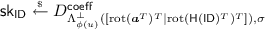
• $\mathsf {SampleLeft}(\varvec{a}, \varvec{b}, u, \varvec{T}_{\varvec{a}}, \sigma ) \rightarrow \varvec{e}$ ([CHKP10]): a randomized algorithm that, given vectors $\varvec{a}, \varvec{b}\in R_q^{k}$ where $\mathrm {rot}(\varvec{a}^T)^T,\mathrm {rot}(\varvec{b}^T)^T \in \mathbb Z_q^{n \times n k}$ are full-rank, an element $u\in R_q$, a matrix $\varvec{T}_{\varvec{a}} \in R^{k \times k}$ such that $\mathrm {rot}(\varvec{T}_{\varvec{a}}) \in \mathbb Z^{nk \times nk }$ is a basis for $\mathrm{\Lambda }^{\perp }(\mathrm {rot}(\varvec{a}^T)^T)$, and a Gaussian parameter $\sigma > ||\mathrm {rot}(\varvec{T}_{\varvec{a}}) ||_\mathsf{GS} \cdot \omega (\sqrt{\log nk})$, outputs a vector $\varvec{e}\in R^{2k}$ sampled from a distribution which is $\mathsf {negl}(n)$-close to $D^\mathsf{coeff}_{\mathrm{\Lambda }_{\phi (u)}^{\perp }([\mathrm {rot}(\varvec{a}^T)^T\vert \mathrm {rot}(\varvec{b}^T)^T]), \sigma }$, i.e., $[\varvec{a}| \varvec{b}] \varvec{e}^T = u$ and $\phi (\varvec{e}) \in \mathbb Z^{2nk}$ is distributed according to $D_{\mathrm{\Lambda }_{\phi (u)}^{\perp }([\mathrm {rot}(\varvec{a}^T)^T\vert \mathrm {rot}(\varvec{b}^T)^T]), \sigma }$.

• $\mathsf {SampleRight}(\varvec{a}, \varvec{g}_b, \varvec{R}, y, u, \varvec{T}_{\varvec{g}_b}, \sigma ) \rightarrow \varvec{e}$ where $\varvec{b}= \varvec{a}\varvec{R}+ y\varvec{g}_{b}$ ([ABB10]): a randomized algorithm that, given vectors $\varvec{a}, \varvec{g}_{b} \in R_q^{k}$ such that $\mathrm {rot}(\varvec{a}^T)^T, \mathrm {rot}(\varvec{g}_{b})$ ⁵ $\in \mathbb Z_q^{n \times nk}$ are full-rank matrices, elements $y\in R_q^*, u\in R_q$, a matrix $\varvec{R}\in R^{k \times k}$, a matrix $\varvec{T}_{\varvec{g}_b} \in R^{k \times k}$ such that $\mathrm {rot}(\varvec{T}_{\varvec{g}_b}) \in \mathbb Z^{nk \times nk}$ is a basis for $\mathrm{\Lambda }^{\perp }(\mathrm {rot}(\varvec{g}_b))$, and a Gaussian parameter $\sigma > s_1(\varvec{R}) \cdot ||\mathrm {rot}(\varvec{T}_{\varvec{g}_b}) ||_\mathsf{GS} \cdot \omega (\sqrt{\log nk})$, outputs a vector $\varvec{e}\in R^{2k}$ sampled from a distribution which is $\mathsf {negl}(n)$-close to $D^\mathsf{coeff}_{\mathrm{\Lambda }_{\phi (u)}^{\perp }([\mathrm {rot}(\varvec{a}^T)^T\vert \mathrm {rot}(\varvec{b}^T)^T]), \sigma }$, i.e., $[\varvec{a}| \varvec{b}] \varvec{e}^T = u$ and $\phi (\varvec{e}) \in \mathbb Z^{2nk}$ is distributed according to $D_{\mathrm{\Lambda }_{\phi (u)}^{\perp }([\mathrm {rot}(\varvec{a}^T)^T\vert \mathrm {rot}(\varvec{b}^T)^T]), \sigma }$.

• ([MP12]:) Let $k \ge \lceil \log _bq \rceil$. There exists a publicly known matrix $\varvec{T}_{\varvec{g}_b}$ such that $\mathrm {rot}(\varvec{T}_{\varvec{g}_b}) \in \mathbb Z^{n k \times n k}$ is a basis for the lattice $\mathrm{\Lambda }^{\perp }(\mathrm {rot}(\varvec{g}_b))$ and $||\mathrm {rot}(\varvec{T}_{\varvec{g}_b}) ||_\mathsf{GS} \le \sqrt{b^2 + 1}$. Furthermore, there exists a deterministic polynomial time algorithm $\varvec{g}_b^{-1}$ which takes input $\varvec{u}\in R_q^{k}$ and outputs $\varvec{R}= \varvec{g}_b^{-1}(\varvec{u})$ such that $\varvec{R}\in [ -b, b ]_{R}^{k \times k}$ and $\varvec{g}_b\varvec{R}= \varvec{u}$.

Note that we abuse the notation $\varvec{g}_{b}^{-1}$ by viewing it as a function rather than a vector. Namely, for any $\varvec{u}\in R_q^k$ there are many choices for $\varvec{R}\in R^{k \times k}$ such that $\varvec{g}_{b} \varvec{R}= \varvec{u}$, and $\varvec{g}_{b}^{-1}(\varvec{u})$ is a function that deterministically outputs a particular short matrix from the possible candidates. Since we have $s_1(\varvec{R}) \le b\cdot nk$ for any $\varvec{R}\in [ -b, b ]_{R}^{k \times k}$, $s_1(\varvec{g}_{b}^{-1}(\varvec{u})) \le bnk$ holds for arbitrary $\varvec{u}\in R_q^k$.

Homomorphic Computation. Let d be a natural number. We introduce the function $\mathsf {PubEval}_d : ( R_{q}^{k} )^d \rightarrow R_{q}^{k}$ as in [Yam16], which takes a set of vectors $\varvec{b}_1, \varvec{b}_2, \ldots , \varvec{b}_d \in R_q^{k}$ as inputs and outputs a vector in $R_{q}^{k}$. This function will be used to hash identities to $R_q^k$ in our lattice-based IBE construction. The function is defined recursively as follows:

$$\begin{aligned} \mathsf {PubEval}_{d}(\varvec{b}_{1},\ldots , \varvec{b}_{d})= {\left\{ \begin{array}{ll} \varvec{b}_1 &{} \text {if}~d=1 \\ \varvec{b}_1 \cdot \varvec{g}_b^{-1}\bigl ( \mathsf {PubEval}_{d-1}(\varvec{b}_2,\ldots , \varvec{b}_d) \bigr ) &{} \text {if} ~d \ge 2. \end{array}\right. } \end{aligned}$$

Lemma 6

Let $y_1, \dots , y_d$ be elements in $R$, $\varvec{a}, \varvec{b}_1, \dots , \varvec{b}_d$ be vectors in $R_q^{k}$ and $\varvec{R}_1, \dots , \varvec{R}_d$ be matrices in $R^{k \times k}$ such that $\varvec{b}_i = \varvec{a}\varvec{R}_i + y_i \varvec{g}_b$ for $i \in [d]$. Furthermore, we assume that $s_1(\varvec{R}_i) \le B, ||\phi (y_i) ||_1 \le \delta$ for $i \in [d]$. Then, there exists an efficient algorithm $\mathsf {TrapEval}_d$ that takes $\varvec{R}_1, \dots , \varvec{R}_d$, $y_1, \dots , y_d$ as inputs and outputs $\varvec{R}' \in R^{k \times k}$ such that

$$\begin{aligned} \mathsf {PubEval}_d(\varvec{b}_1, \dots , \varvec{b}_d) = \varvec{a}\varvec{R}' + y_1\cdots y_d\varvec{g}_b\in R_q^{k} \end{aligned}$$

and $s_1(\varvec{R}') \le B \delta ^{d-1} + Bbnk \big ( \frac{\delta ^{d-1} -1}{\delta - 1}\big )$.

3.4 Other Facts

Lemma 7 (Expansion of Coefficients)

Let $c_1, c_2, B_1, B_2 \in \mathbb {N}$. Let also $u= u_0 + u_1 X + \cdots u_{c_1-1}X^{c_1-1}\in R$ and $v= v_0 + v_1 X + \cdots v_{c_2-1}X^{c_2-1} \in R$ be ring elements. We further assume that $c_1 + c_2 < n$ and $\Vert \phi (u) \Vert _\infty < B_1$ and $\Vert \phi (v) \Vert _\infty < B_2$. Then we have $\Vert \phi ( uv) \Vert _\infty \le \min \{c_1,c_2\} \cdot B_1 B_2$.

The following Lemma addresses a general statement for bounding the success probability of an adversary engaging with the security game of IBE. In more detail, when the partitioning technique is used to prove security, the guess returned by the adversary is correlated with the key extraction queries it has made. Therefore, we need to argue with care to obtain a meaningful bound on the success probability that holds for arbitrary key extraction queries.

Lemma 8

(Implicit in [BR09, Yam16]). Let us consider an IBE scheme and an adversary $\mathcal {A}$ that breaks adaptive security (adaptively-anonymous security) with advantage $\epsilon$. Let us also consider a map $\gamma$ that maps a sequence of identities to a value in [0, 1]. We consider the following experiment. We first execute the security game for $\mathcal {A}$. Let $\mathsf {ID}^\star$ be the challenge identity and $\mathsf {ID}_1,\ldots , \mathsf {ID}_Q$ be the identities for which key extraction queries were made. We denote $\mathbb {ID}= (\mathsf {ID}^\star , \mathsf {ID}_1, \ldots , \mathsf {ID}_Q)$. At the end of the game, we set $\mathsf {coin}' \in \{ 0,1\}$ as $\mathsf {coin}' = \widehat{\mathsf {coin}}$ with probability $\gamma (\mathbb {ID})$ and with probability $1- \gamma (\mathbb {ID})$. Then, the following holds.

$$\begin{aligned} \left| \Pr [\mathsf {coin}' = \mathsf {coin}] - \frac{1}{2} \right| \ge \gamma _{\min }\cdot \epsilon - \frac{\gamma _{\max } - \gamma _{\min } }{2} \end{aligned}$$

where $\gamma _{\min }$ (resp. $\gamma _{\max }$) is the maximum (resp. minimum) of $\gamma (\mathbb {ID})$ taken over all possible $\mathbb {ID}$.

Injective map. Let d and $\kappa$ be some integers. Furthermore, let $\ell$ be $\ell = \lceil \kappa ^{1/d} \rceil$. Then, an element of $[1,\kappa ]$ can be written as an element of $[1,\ell ]^d$ using some canonical map. Furthermore, it is also possible to write a subset of $[1,\kappa ]$ as a subset of $[1,\ell ]^d$ by naturally extending the canonical map. By identifying a bit string in $\{ 0,1 \}^\kappa$ with a subset of $[1,\kappa ]$ (for example, by regarding the former as the indicator vector of a subset of $[1,\kappa ]$), we can define an efficiently computable injective map S that maps a bit string $\mathsf {ID}\in \{ 0,1 \}^\kappa$ to a subset $S(\mathsf {ID})$ of $[1,\ell ]^d$.

3.5 Core Lemma for Our Partitioning

We make a general statement concerning the partitioning technique for IBEs, which we use during the security analysis for both our lattice and bilinear map based constructions. Namely, we use the following Lemma in order to argue that the probability of the hash value for identities corresponding to the key extraction queries being invertible and the hash value for the challenge identity being zero is non-negligible.

Lemma 9

Let $\nu , \mu , d, Q \ge 1$ be any integers. Let $\varPhi$ be a ring and $\varOmega _1,\ldots , \varOmega _\nu$ be a set of fields equipped with homomorphisms $\pi _j: \varPhi \rightarrow \varOmega _j$ for $j\in [\nu ]$. Assume that the map $\varPi$ defined as $\varPi : \varPhi \ni y \mapsto (\pi _1(y), \ldots , \pi _{\nu }(y)) \in \varOmega _1\times \cdots \times \varOmega _\nu$ is an isomorphism. Let $S_0$ and $S_1$ be subsets of $\varPhi$ with finite cardinality. Let us consider a set of multivariate polynomials $f_i(Y_1,\ldots , Y_\mu ) \in \varPhi [Y_1,\ldots , Y_{\mu }]$ for $i\in [0,Q]$ We further assume the following properties:

• 1. The map $\pi _j$ is injective on $S_1$ for all $j\in [\nu ]$.

• 2. We have $\pi _j( f_0 ) - \pi _j( f_i )$ is a non-zero polynomial with degree d for all $i\in [Q]$ and $j\in [\nu ]$. Here $\pi _j$ is extended to $\pi _j: \varPhi [X] \rightarrow \varOmega _j[X]$ in a natural way.

• 3. We have $S_0 \supseteq \cup _{i\in [0,Q]} \{ - f_i(y_1,\ldots ,y_\mu ) | y_1,\ldots , y_\mu \in S_1 \}$.

Then, for and , we have

$$\begin{aligned} \frac{1}{| S_0 |} \left( 1 - \frac{d\nu Q}{|S_1|} \right) \le \gamma \le \frac{1}{|S_0|} \end{aligned}$$

where we denote

$$\begin{aligned} \gamma = \Pr _{y_0, \varvec{y}'} [~ y_0 + f_0(\varvec{y}')=0 ~ \wedge ~ y_0 + f_1(\varvec{y}')\in \varPhi ^* ~ \wedge \cdots \wedge ~ y_0 + f_Q(\varvec{y}')\in \varPhi ^*], \end{aligned}$$

$\varvec{y}' = (y_1,\ldots ,y_\mu )$, and $\varPhi ^* = \varPi ^{-1}( \varOmega _1^* \times \cdots \times \varOmega _\nu ^* )$.

4 Construction from RLWE

In this section, we show our IBE scheme from the RLWE assumption. Let d be a (flexible) constant number. In addition, let the identity space of the scheme be $\mathcal {ID} = \{ 0,1 \}^{\kappa }$ for some $\kappa \in \mathbb N$ and the message space be $\{ 0,1 \}^n \subset R$.⁶ For our construction, we consider an efficiently computable injective map S that maps an identity $\mathsf {ID}\in \{ 0, 1 \}^\kappa$ to a subset $S(\mathsf {ID})$ of $[1, \ell ]^d$, where $\ell = \lceil \kappa ^{1/d} \rceil$. Such a map can be constructed easily as we explained in Sect. 3.4. Let $n \mathrel {\mathop :}=n(\lambda )$, $b\mathrel {\mathop :}=b(n)$, $\rho \mathrel {\mathop :}=\rho (n)$, $m \mathrel {\mathop :}=2n$, $k \mathrel {\mathop :}=k(n)$, $q \mathrel {\mathop :}=q(n)$, $\ell \mathrel {\mathop :}=\ell (n)$, $\alpha \mathrel {\mathop :}=\alpha (n)$, $\alpha ' \mathrel {\mathop :}=\alpha '(n)$, and $\sigma \mathrel {\mathop :}=\sigma (n)$ be parameters that are specified later. Let also $\varPhi _m(X) = X^{n}+1$ be the mth cyclotomic polynomial and $R=\mathbb {Z}[X]/(\varPhi _m(X))$.

• $\mathsf {Setup}(1^\lambda )$: On input $1^\lambda$, it first runs to obtain $\varvec{a}\in R_q^{ k }$ and $\varvec{T}_{\varvec{a}} \in R^{k \times k}$. It also picks , for $(i,j) \in [d] \times [ \ell ]$ and outputs

  $$\begin{aligned} \mathsf {mpk}= (\varvec{a}, \varvec{b}_0, \{ \varvec{b}_{i,j} \}_{(i,j)\in [d] \times [\ell ]}, u) \quad \text{ and } \quad \mathsf {msk}= \varvec{T}_{\varvec{a}}. \end{aligned}$$

In the following, we use a deterministic function $\mathsf {H}: \mathcal {ID}\rightarrow R_q^k$ defined as

$$\begin{aligned} \mathsf {H}(\mathsf {ID})= \varvec{b}_0 + \sum _{(j_1,\ldots , j_d )\in S(\mathsf {ID})} \mathsf {PubEval}_d(\varvec{b}_{1,j_1}, \varvec{b}_{2, j_2}, \ldots , \varvec{b}_{d,j_d}) \in R_q^{k}. \end{aligned}$$

• $\mathsf {KeyGen}(\mathsf {mpk}, \mathsf {msk}, \mathsf {ID})$: It first computes $\mathsf {H}(\mathsf {ID})$ and picks $\varvec{e}\in R^{2k}$ such that

  $$\begin{aligned}{}[ \varvec{a}| \mathsf {H}(\mathsf {ID}) ] \cdot \varvec{e}^T = u \end{aligned}$$

  using $\mathsf {SampleLeft}(\varvec{a}, \mathsf {H}(\mathsf {ID}), u, \mathbf {T}_{\varvec{a}}, \sigma ) \rightarrow \varvec{e}$. It returns $\mathsf {sk}_\mathsf {ID}= \varvec{e}$.

• $\mathsf {Encrypt}(\mathsf {mpk}, \mathsf {ID}, \mathsf {M})$: To encrypt a message $\mathsf {M}\in \{ 0,1 \}^n \subset R$, it first picks , , . Then it computes

  $$\begin{aligned} c_0 = su + x_0 + \lfloor q/2 \rceil \cdot \mathsf {M}, \quad \varvec{c}_1 = s[ \varvec{a}| \mathsf {H}(\mathsf {ID}) ] + [ \varvec{x}_1 | \varvec{x}_2 ]. \end{aligned}$$

  Finally, it outputs the ciphertext $C=(c_0,\varvec{c}_1) \in R_q \times R_q^{2k}$.

• $\mathsf {Decrypt}(\mathsf {mpk},\mathsf {sk}_\mathsf {ID}, C )$: To decrypt a ciphertext $C=(c_0, \varvec{c}_1)$ using a private key $\mathsf {sk}_\mathsf {ID}= \varvec{e}$, it computes $\left( \lfloor (2/q) \cdot \phi ( c_0 - \varvec{c}_1 \varvec{e}^T ) \rceil \mod 2 \right) = m.$ Here, the rounding function $\lfloor \cdot \rceil$ is applied componentwise.

4.1 Correctness and Parameter Selection

The following lemma addresses the correctness of the scheme.

Lemma 10 (Correctness)

[Correctness] Assume $\alpha q \omega (\sqrt{\log n}) + \sqrt{nk} \alpha ' \sigma \omega (\sqrt{\log nk}) \le q/5$ holds with over whelming probability. Then the above scheme has negligible decryption error.

Parameter selection. We refer the precise requirements for the parameter selection to the full version. One concrete selection for the parameters is as follows:

$$\begin{aligned} k&= 8d + 12,&q&= n^{2d + 3},&b&= \rho = n^{\frac{1}{4}}, \nonumber \\ \sigma&= n^{d} \cdot \omega (\log n) ,&\alpha&= n^{-2d - \frac{3}{8}} \cdot \omega (\log ^{2} n)^{-1},&\alpha '&= n^{d + \frac{5}{2}} \cdot \omega (\log ^{\frac{3}{4}} n)^{-1}, \end{aligned}$$

where d is a (flexible) constant which may be set very small (e.g., $d=2$ or 3) in a typical setting and the length $\kappa$ of the identities $\mathsf {ID}$ is set as n. This specific instantiation is denoted as the Type 2 IBE scheme in Sect. 6. Table 1. Furthermore, the other concrete instantiation provided only in the full version, where we set $b=2$ and $k = O(\log n)$, is denoted as the Type 1 IBE scheme.

4.2 Security Proof for the Scheme

The following theorem addresses the security of the scheme. The proof proceeds in a similar manner as in [Yam16], but we incorporate several novel ideas as we explained in Sect. 2.

Theorem 2

The above IBE scheme is adaptively-anonymous secure assuming $\mathsf {RLWE}_{n,k+1,q, D^\mathsf{coeff}_{\mathbb {Z}^n, \alpha q}}$ is hard, where the ciphertext space is $\mathcal {C}= R_q \times R_q^{2k}$.

Proof

Let $\mathcal {A}$ be a PPT adversary that breaks the adaptively-anonymous security of the scheme. In addition, let $\epsilon = \epsilon (n)$ and $Q = Q(n)$ be its advantage and the upper bound of the number of key extraction queries, respectively.

Since $\mathcal {A}$ is PPT and $\lambda$ and n are polynomially related (namely, $n=O(\lambda ^{\delta })$ for some constant $\delta$), there exists a constant number $c_1 \in \mathbb {N}$ such that $4(dQ+ 1) \le n^{c_1}$ for all n that are sufficiently large. Similarly, since $\mathcal {A}$ breaks the security of the scheme, there exists $c_2 \in \mathbb {N}$ such that $2\epsilon \ge n^{-c_2}$ holds for infinitely many n. By setting $c= c_1 + c_2$, we have that

$$\begin{aligned} 4dQ \le n^c~ \text{ for } \text{ all } n\in \mathbb {N} \quad \text{ and } \quad \frac{\epsilon }{2(dQ+1)} \ge \frac{1}{n^c} \quad \text{ for } \text{ infinitely } \text{ many } n\in \mathbb {N}. \end{aligned}$$

(8)

In the proof, we will assume $d(c- 1) < n$. Since both $c$ and d are constant numbers, this holds for sufficiently large n.

We show the security of the scheme via the following games. In each game, a value $\mathsf {coin}' \in \{ 0,1 \}$ is defined. While it is set $\mathsf {coin}' = \widehat{\mathsf {coin}}$ in the first game, these values might be different in the later games. In the following, we define $X_i$ to be the event that $\mathsf {coin}' = \mathsf {coin}$.

• $\mathsf {Game}_{0}$: This is the real security game. In the challenge phase, the challenge ciphertext is set as if $\mathsf {coin}= 1$. Otherwise, it is set as $C^\star \leftarrow \mathsf {Encrypt}(\mathsf {mpk}, \mathsf {ID}, \mathsf {M})$, where $\mathsf {M}$ is the message chosen by $\mathcal {A}$. At the end of the game, $\mathcal {A}$ outputs a guess $\widehat{\mathsf {coin}}$ for $\mathsf {coin}$. Finally, the challenger sets $\mathsf {coin}' = \widehat{\mathsf {coin}}$. By definition, we have

  $$\begin{aligned} \left| \Pr [X_0] - \frac{1}{2} \right| = \left| \Pr [\mathsf {coin}' = \mathsf {coin}] - \frac{1}{2} \right| = \left| \Pr [\widehat{\mathsf {coin}} = \mathsf {coin}] - \frac{1}{2} \right| = \epsilon . \end{aligned}$$

• $\mathsf {Game}_{1}$: For integers $t_0, t_1 \in \mathbb {Z}$ such that $t_0 \le t_1$ and positive integer $c \in \mathbb N$, let us denote $[t_0, t_1]_{R, c}$ as

  

  In words, $[t_0,t_1]_{R, c}$ denotes the set of polynomials of degree less then $c-1$ with all of its coefficients in the interval $[t_0,t_1]$. Note that c is the constant defined in Eq. (8). In this game, we change $\mathsf {Game}_0$ so that the challenger performs the following additional step at the end of the game. First, the challenger picks $\varvec{y}=(y_0, \{ y_{i,j} \}_{(i,j)\in [d,\ell ]})$ as

  

  (9)

  for $(i,j)\in [d]\times [\ell ]$. Recall $\kappa$ is the length of the identities. We then define a function $\mathsf {F}_{\varvec{y}} : \mathcal {ID}\rightarrow R_q$ as follows:

  $$\begin{aligned} \mathsf {F}_{\varvec{y}}(\mathsf {ID})= y_0 + \sum _{(j_1, \ldots , j_d)\in S(\mathsf {ID})} y_{1,j_1}\cdots y_{d,j_d}. \end{aligned}$$

  Then the challenger checks whether the following condition holds:

  $$\begin{aligned} \mathsf {F}_{\varvec{y}}(\mathsf {ID}^\star )=0 ~ \wedge ~ \mathsf {F}_{\varvec{y}}(\mathsf {ID}_1) \in R_q^* ~ \wedge ~ \cdots ~ \wedge ~ \mathsf {F}_{\varvec{y}}(\mathsf {ID}_Q) \in R_q^*, \end{aligned}$$

  (10)

  where $\mathsf {ID}^\star$ is the challenge identity, and $\mathsf {ID}_1,\ldots , \mathsf {ID}_Q$ are identities for which $\mathcal {A}$ has made key extraction queries. If it does not hold, the challenger ignores the output $\widehat{\mathsf {coin}}$ of $\mathcal {A}$, and sets . In this case, we say that the challenger aborts. If condition (10) holds, the challenger sets $\mathsf {coin}' = \widehat{\mathsf {coin}}$. As we will show in Lemma 11, we have

  $$\begin{aligned} \left| \Pr [X_1] -\frac{1}{2} \right| \ge \frac{ 1 }{ ( \kappa c^d n^d )^{(c- 1)d + 1} } \left( \frac{\epsilon }{2} - \frac{dQ}{n^c} \right) . \end{aligned}$$

  So as not to interrupt the proof of Theorem 2, we intentionally skip the proof for the time being.

• $\mathsf {Game}_{2}$: In this game, we change the way $\varvec{b}_0$ and $\varvec{b}_{i,j}$ are chosen. At the beginning of the game, the challenger picks for $(i,j)\in [d]\times [\ell ]$. It also picks $\varvec{y}$ as in $\mathsf {Game}_1$. Then, $\varvec{a}$, $\varvec{b}_0$, and $\varvec{b}_{i,j}$ are defined as

  $$\begin{aligned} \varvec{b}_0=\varvec{a}\varvec{R}_0 + y_0 \varvec{g}_b, \qquad \varvec{b}_{i,j}=\varvec{a}\varvec{R}_{i,j} + y_{i,j} \varvec{g}_b, \end{aligned}$$

  (11)

  for $(i,j) \in [d] \times [\ell ]$. The rest of the game is the same as in $\mathsf {Game}_1$. Now, we bound $\left| \Pr [X_2]-\Pr [X_1] \right|$. By Lemma 4, the distributions

  $$\begin{aligned} \bigl (\varvec{a}, \varvec{a}\varvec{R}_0+ y_0 \varvec{g}_b, \{ \varvec{a}\varvec{R}_{i,j}+y_{i,j}\varvec{g}_b\}_{(i,j)\in [d]\times [\ell ]} \bigr ) ~~ \text{ and } ~~ \bigl ( \varvec{a}, \varvec{b}_0, \{ \varvec{b}_{i,j} \}_{(i,j)\in [d]\times [\ell ]} \bigr ) \end{aligned}$$

  are $\mathsf {negl}(n)$-close, where . Thus, we have $\left| \Pr [X_1] - \Pr [X_2] \right| = \mathsf {negl}(n).$

• $\mathsf {Game}_{3}$: Recall that in the previous game, the challenger aborts at the end of the game if condition (10) is not satisfied. In this game, we change the game so that the challenger aborts as soon as the abort condition becomes true. Since this is only a conceptual change, we have $\Pr [X_2]=\Pr [X_3].$

Before describing the next game, we define $\varvec{R}_{\mathsf {ID}} \in R^{k \times k}$ for an identity $\mathsf {ID}\in \mathcal {ID}$ as

$$\begin{aligned} \varvec{R}_{\mathsf {ID}}= \varvec{R}_0 + \sum _{(j_1, \ldots , j_d)\in S(\mathsf {ID})} \mathsf {TrapEval}_d(\varvec{R}_{1,j_1},\ldots , \varvec{R}_{d,j_d}, y_{1,j_1}, \ldots , y_{d,j_d}). \end{aligned}$$

(12)

Note that by the definition of $\varvec{R}_\mathsf {ID}$, $\mathsf {H}(\mathsf {ID})$, $\mathsf {PubEval}$ and $\mathsf {TrapEval}$ (Lemma 6) we have

$$\begin{aligned} \mathsf {H}(\mathsf {ID})&= \varvec{b}_0 + \sum _{(j_1,\ldots , j_d )\in S(\mathsf {ID})} \mathsf {PubEval}_d(\varvec{b}_{1,j_1} \varvec{b}_{2, j_2}, \ldots , \varvec{b}_{d,j_d}) \nonumber \\&= \varvec{a}\varvec{R}_\mathsf {ID}+ \mathsf {F}_{\varvec{y}}(\mathsf {ID}) \varvec{g}_b. \end{aligned}$$

(13)

Since , from Lemma 2 we have $s_1(\varvec{R}_0), s_1(\varvec{R}_{i, j}) \le B$ with all but negligible probability where $B = C' \cdot \rho \sqrt{n}(\sqrt{k} + \omega (\sqrt{\log n}))$ for some positive absolute constant $C'$. Furthermore, we have $||y_{i,j} ||_1 \le cn$ from Eq. (9). Therefore by Lemma 6, we have

$$\begin{aligned} s_1( \varvec{R}_{\mathsf {ID}} )\le & {} s_1( \varvec{R}_0 ) + \sum _{(j_1, \ldots , j_d)\in S(\mathsf {ID})} s_1( \mathsf {TrapEval}_d(\varvec{R}_{1,j_1},\ldots , \varvec{R}_{d,j_d}, y_{1,j_1}, \ldots , y_{d,j_d}) ) \nonumber \\\le & {} B \bigg ( 1 + \kappa (cn)^{d-1} + \kappa bnk \frac{(cn)^{d-1}-1}{cn -1 } \bigg ), \end{aligned}$$

(14)

for any $\mathsf {ID}\in \mathcal {ID}$ with all but negligible probability.

• $\mathsf {Game}_{4}$: In this game, we change the way the vector $\varvec{a}$ is sampled. Namely, $\mathsf {Game}_4$ challenger picks instead of generating it with a trapdoor. By Lemma 5, this makes only negligible difference. Furthermore, we also change the way the key extraction queries are answered. When $\mathcal {A}$ makes a key extraction query for an identity $\mathsf {ID}$, the challenger first computes $\varvec{R}_\mathsf {ID}$ as in Eq. (12). It aborts if $\mathsf {F}_{\varvec{y}}(\mathsf {ID}) \not \in R_q^*$ as in the previous game and runs

  $$\begin{aligned} \mathsf {SampleRight}(\varvec{a}, \varvec{g}_b, \varvec{R}_\mathsf {ID}, \mathsf {F}_\mathbf {y}(\mathsf {ID}), u, \mathbf {T}_{\varvec{g}_b}, \sigma ) \rightarrow \varvec{e}, \end{aligned}$$

  otherwise. Note that in the previous game the private key was sampled as

  $$\begin{aligned} \mathsf {SampleLeft}(\varvec{a},\mathsf {H}(\mathsf {ID}),u, \mathbf {T}_{\varvec{a}}, \sigma ) \rightarrow \varvec{e}. \end{aligned}$$

  By Eq. (14) and for our choice of $\sigma$, the output distribution of $\mathsf {SampleRight}$ is $\mathsf {negl}(n)$-close to $D^\mathsf{coeff}_{\mathrm{\Lambda }_{\phi (u)}^{\perp }([\mathrm {rot}(\varvec{a}^T)^T\vert \mathrm {rot}(\mathsf {H}(\mathsf {ID})^T)^T]), \sigma }$. Furthermore, by the choice of $\sigma$, this distribution is $\mathsf {negl}(n)$-close to the output distribution of $\mathsf {SampleLeft}$. Therefore, the above change alters the view of $\mathcal {A}$ only negligibly. Thus, we have $\left| \Pr [X_3] - \Pr [X_4] \right| = \mathsf {negl}(n).$

• $\mathsf {Game}_{5}$: In this game, we change the way the challenge ciphertext is created when $\mathsf {coin}=0$. Recall in the previous games when $\mathsf {coin}= 0$, we created a valid challenge ciphertext as in the real scheme. If $\mathsf {coin}=0$ and $\mathsf {F}_{\varvec{y}}(\mathsf {ID}^\star )=0$ (i.e., if it does not abort), to create the challenge ciphertext $\mathsf {Game}_5$ challenger first picks and and computes $\varvec{v}= s\varvec{a}+ \varvec{x}\in R^k$. It then runs the algorithm

  $$\begin{aligned} \mathsf {ReRand}\left( \mathrm {rot}\bigl ( [\varvec{I}_k | \varvec{R}_{\mathsf {ID}^\star }] \bigr ), \phi ( \varvec{v}), \alpha q, \frac{\alpha '}{2\alpha q} \right) \rightarrow \mathbf {c}\in \mathbb {Z}_q^{2nk} \end{aligned}$$

  from Lemma 1, where $\varvec{I}_{k} \in R^{k\times k}$ is the identity matrix of size $k\times k$. Finally, it picks and sets the challenge ciphertext as

  $$\begin{aligned} C^\star = \left( ~ c_0 = v_0 + \lfloor q/2 \rceil \cdot \mathsf {M}, ~ \varvec{c}_1 = \phi ^{-1}(\mathbf {c}) ~ \right) \in R_q \times R_q^{2k}, \end{aligned}$$

  (15)

  where $v_0 = su + x_0$ and $\mathsf {M}$ is the message chosen by $\mathcal {A}$. We claim that this change alters the view of $\mathcal {A}$ only negligibly. To show this, observe that the input to $\mathsf {ReRand}$ is $\mathrm {rot}\big ([\varvec{I}_k | \varvec{R}_{\mathsf {ID}^\star }] \big ) \in \mathbb Z_q^{nk \times 2nk}$ and

  $$\begin{aligned} \phi (\varvec{v}) = \phi (s \varvec{a}+ \varvec{x}) = \phi (s) \mathrm {rot}(\varvec{a}) + \phi (\varvec{x}) \in \mathbb Z_q^{nk}, \end{aligned}$$

  where $\phi (\varvec{x})$ is distributed as . Therefore, by the property of $\mathsf {ReRand}$ and our choice of $\alpha$ and $\alpha '$, the output $\mathbf {c}\in \mathbb {Z}^{2nk}_q$ is

  $$\begin{aligned} \mathbf {c}= & {} \Big ( \phi (s) \mathrm {rot}(\varvec{a}) \Big ) \cdot \mathrm {rot}\big ([\varvec{I}_k | \varvec{R}_{\mathsf {ID}^\star }] \big ) + \mathbf {x}' \\= & {} \phi (s) \cdot \mathrm {rot}\big ([\varvec{a}| \mathsf {H}(\mathsf {ID}^\star )] \big ) + \mathbf {x}' \\= & {} \phi \bigl (s\bigl [ \varvec{a}| \mathsf {H}(\mathsf {ID}^\star ) \bigr ] \bigr ) + \mathbf {x}', \end{aligned}$$

  where the distribution of $\mathbf {x}'$ is within negligible distance from due to Lemma 1. Here, we use the fact that $\mathsf {H}(\mathsf {ID}^\star ) = \varvec{a}\varvec{R}_{\mathsf {ID}^\star }$ holds since $\mathsf {F}_{\varvec{y}}(\mathsf {ID}^\star ) = 0$. It can be readily seen that the distribution of $\varvec{c}_1 = \phi ^{-1}(\mathbf {c})$ in $\mathsf {Game}_5$ is statistically close to that in $\mathsf {Game}_4$. Therefore, we conclude that $\left| \Pr [X_4] - \Pr [X_5] \right| = \mathsf {negl}(n).$

• $\mathsf {Game}_{6}$: In this game, we change the way the challenge ciphertext is created when $\mathsf {coin}=0$. If $\mathsf {coin}=0$ and the abort condition is not satisfied, to create the challenge ciphertext for identity $\mathsf {ID}^\star$ and message $\mathsf {M}$, $\mathsf {Game}_6$ challenger first picks , and , and runs

  $$\begin{aligned} \mathsf {ReRand}\left( \mathrm {rot}\big ( [ \varvec{I}_{k } | \varvec{R}_{\mathsf {ID}^\star }] \big ), \phi ( \varvec{v}), \alpha q, \frac{\alpha '}{2\alpha q} \right) \rightarrow \mathbf {c}\in \mathbb {Z}_q^{2nk}, \end{aligned}$$

  (16)

  where $\varvec{v}= \varvec{v}' + \varvec{x}$. Then, the challenge ciphertext is set as in Eq. (15). As we will show in Lemma 12, assuming $\mathsf {RLWE}_{n,k+1,q,D^\mathsf{coeff}_{\mathbb {Z}^n, \alpha q}}$ is hard, we have $\left| \Pr [X_5]-\Pr [X_6] \right| =\mathsf {negl}(n).$

• $\mathsf {Game}_{7}$: In this game, we further change the way the challenge ciphertext is created. When $\mathsf {coin}=0$ and the abort condition is not satisfied, the challenge ciphertext for $\mathsf {ID}^\star$ is created as

  $$\begin{aligned} C^\star = \left( ~ c_0 = v_0 + \lfloor q/2 \rceil \cdot \mathsf {M}, ~ \varvec{c}_1 = [ \varvec{v}' | \varvec{v}' \varvec{R}_{\mathsf {ID}^\star }] + [\varvec{x}_1 | \varvec{x}_2 ] ~ \right) \in R_q \times R^{2k}, \end{aligned}$$

  where , and . We claim that this change alters the view of $\mathcal {A}$ only negligibly. This can be seen by a similar argument to that we made in the step from $\mathsf {Game}_3$ to $\mathsf {Game}_4$. We first observe that in $\mathsf {Game}_6$ the input to $\mathsf {ReRand}$ is $\mathrm {rot}\big ([\varvec{I}_k | \varvec{R}_{\mathsf {ID}^\star }] \big )~\in ~\mathbb Z_q^{nk \times 2nk}$ and

  $$\begin{aligned} \phi (\varvec{v}) = \phi ( \varvec{v}' + \varvec{x}) = \phi ( \varvec{v}') + \phi (\varvec{x}) \in \mathbb Z_q^{nk}, \end{aligned}$$

  (17)

  where $\phi (\varvec{x})$ is distributed as $D_{\mathbb {Z}^{nk}, \alpha q}$. Therefore, the output $\mathbf {c}\in \mathbb {Z}^{2nk}_q$ of $\mathsf {ReRand}$ is

  $$\begin{aligned} \mathbf {c}= \phi (\varvec{v}' ) \cdot \mathrm {rot}\big ( [\varvec{I}_k | \varvec{R}_{\mathsf {ID}^\star }] \big ) + \mathbf {x}' = \phi \big ( [\varvec{v}' | \varvec{v}' \varvec{R}_{\mathsf {ID}^\star } ] \big ) + \mathbf {x}', \end{aligned}$$

  where the distribution of $\mathbf {x}'$ is within negligible distance from due to Lemma 1. Hence, the distribution of $\varvec{c}_1 = \phi ^{-1}(\mathbf {c})$ in $\mathsf {Game}_6$ is statistically close to that in $\mathsf {Game}_7$. Therefore, we have $\left| \Pr [X_6] - \Pr [X_7] \right| = \mathsf {negl}(n).$

• $\mathsf {Game}_{8}$: In this game, we change the way the key extraction queries are answered. Instead of running $\mathsf {SampleLeft}$ or $\mathsf {SampleRight}$, the (possibly inefficient) challenger directly picks a secret key $\mathsf {sk}_\mathsf {ID}$ for identity $\mathsf {ID}$ as without using $\varvec{R}_{\mathsf {ID}}$. Similarly to the change from $\mathsf {Game}_3$ to $\mathsf {Game}_4$, by the choice of $\sigma$ and Eq. (14), this alters the view of $\mathcal {A}$ only negligibly. Therefore, we have $\left| \Pr [X_7] - \Pr [X_8] \right| = \mathsf {negl}(n).$ Note that this is only a conceptual game in order to get rid of any (negligible) correlation between the secret key and $\varvec{R}_{\mathsf {ID}}$ so as not to interfere with the statistical argument using $\varvec{R}_{\mathsf {ID}^\star }$ in the following game.

• $\mathsf {Game}_{9}$: In this game, we change the challenge ciphertext to be a random vector, regardless of whether $\mathsf {coin}=0$ or $\mathsf {coin}=1$. Namely, $\mathsf {Game}_9$ challenger generates the challenge ciphertext $C^\star = (c_0,\varvec{c}_1)$ as

  

  We now proceed to bound $\left| \Pr [X_8] - \Pr [X_9] \right|$. Since $\mathsf {Game}_8$ and $\mathsf {Game}_9$ differ only in the creation of the challenge ciphertext when $\mathsf {coin}= 0$, we focus on this case. First, it is easy to see that $c_0$ is uniformly random over $R_q$ in both of $\mathsf {Game}_8$ and $\mathsf {Game}_9$. Therefore, we only need to show that the distribution of $\varvec{c}_1$ in $\mathsf {Game}_8$ is $\mathsf {negl}(n)$-close to the uniform distribution over $R_q^{2k}$. To see this, it suffices to show that $[ \varvec{v}' | \varvec{v}' \varvec{R}_{\mathsf {ID}^\star } ]$ is distributed statistically close to the uniform distribution over $R_q^{2k}$. First, observe that the following distributions are $\mathsf {negl}(n)$-close:

  $$\begin{aligned} (\varvec{a}, \varvec{a}\varvec{R}_0, \varvec{v}', \varvec{v}' \varvec{R}_0) \approx (\varvec{a}, \varvec{a}', \varvec{v}', \varvec{v}'' ) \approx (\varvec{a}, \varvec{a}\varvec{R}_0, \varvec{v}', \varvec{v}'' ), \end{aligned}$$

  (18)

  where , , . It can be seen that the first and the second distributions are $\mathsf {negl}(n)$-close, by applying Lemma 4 for $[ \varvec{a}; \varvec{v}' ] \in R_q^{2 \times k}$ and $\varvec{R}_0$. It can also be seen that the second and the third distributions are $\mathsf {negl}(n)$-close, by applying the same lemma for $\varvec{a}$ and $\varvec{R}_0$. From the above, the following distributions are statistically close:

  $$\begin{aligned}&(\varvec{a}, \varvec{a}\varvec{R}_0, \varvec{v}', \varvec{v}' \varvec{R}_{\mathsf {ID}^\star } )\\= & {} \left( \varvec{a}, \varvec{a}\varvec{R}_0, \varvec{v}', \varvec{v}' \left( \varvec{R}_0 + \varvec{R}'_{\mathsf {ID}^\star } \right) \right) \\\approx & {} \left( \varvec{a}, \varvec{a}\varvec{R}_0, \varvec{v}', \varvec{v}'' + \varvec{v}' \varvec{R}'_{\mathsf {ID}^\star } \right) \\\approx & {} (\varvec{a}, \varvec{a}\varvec{R}_0, \varvec{v}', \varvec{v}'' ) \end{aligned}$$

  where , , 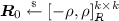, and

  $$\begin{aligned} \varvec{R}'_{\mathsf {ID}^\star } := \sum _{(j_1, \ldots , j_d)\in S(\mathsf {ID})} \mathsf {TrapEval}_d(\varvec{R}_{1,j_1},\ldots , \varvec{R}_{d,j_d}, y_{1,j_1}, \ldots , y_{d,j_d}). \end{aligned}$$

  The second and the third distributions above are $\mathsf {negl}(n)$-close by Eq. (18). Note that we intentionally ignored all the $\varvec{a}\varvec{R}_{i, j}$ terms to keep the argument simple, since focusing on the $\varvec{a}\varvec{R}_0$ term is enough to prove randomness of $[ \varvec{v}' | \varvec{v}' \varvec{R}_{\mathsf {ID}^\star } ]$. Therefore, we conclude that $\left| \Pr [X_8] - \Pr [X_9] \right| = \mathsf {negl}(n).$

Analysis. From the above, we have

$$\begin{aligned} \left| \Pr [X_9] -\frac{1}{2} \right|= & {} \left| \Pr [X_1] -\frac{1}{2} + \sum ^{8}_{i=1} \left( \Pr [X_{i+1}] -\Pr [X_i] \right) \right| \nonumber \\\ge & {} \left| \Pr [X_1] -\frac{1}{2}\right| - \sum ^{8}_{i=1} \left| \Pr [X_{i+1}] -\Pr [X_i] \right| \nonumber \\\ge & {} \frac{ 1}{ ( \kappa c^d n^d )^{(c- 1)d + 1} } \left( \frac{\epsilon }{2} - \frac{dQ}{n^c} \right) - \mathsf {negl}(n) \nonumber \\= & {} \frac{1 }{\mathsf {poly}(n)} \left( \frac{\epsilon }{2} - \frac{dQ}{n^c} \right) - \mathsf {negl}(n) \end{aligned}$$

(19)

where the last equality follows from the facts that $c$ and d are constants and $\kappa = \mathsf {poly}(n)$. Since the challenge ciphertext is independent from the value of $\mathsf {coin}$ in $\mathsf {Game}_9$, we have $\Pr [X_9]=1/2$ and thus $\left| \Pr [X_9] - 1/2 \right| =0$. Therefore, we have that $\epsilon /2 - dQ/n^c$ is negligible. However, by Eq. (8),

$$\begin{aligned} \frac{\epsilon }{2} - \frac{dQ}{n^c} \ge \frac{dQ+1}{n^c} - \frac{dQ}{n^c} = \frac{1}{n^c} \end{aligned}$$

holds for infinitely many n, which is a contradiction.

To complete the proof of Theorem 2, it remains to prove Lemmas 11 and 12.

Lemma 11

For any PPT adversary $\mathcal {A}$, we have

$$\begin{aligned} \left| \Pr [X_1] -\frac{1}{2} \right| \ge \frac{ 1 }{ ( \kappa c^d n^d )^{(c- 1)d + 1} } \left( \frac{\epsilon }{2} - \frac{dQ}{n^c} \right) . \end{aligned}$$

Proof

For a sequence of identities $\mathbb {ID}=(\mathsf {ID}^\star , \mathsf {ID}_1,\ldots , \mathsf {ID}_Q) \in \mathcal {ID}^{Q+1}$, we define $\gamma (\mathbb {ID})$ as

$$\begin{aligned} \gamma (\mathbb {ID})= \Pr _{\varvec{y}}[ \mathsf {F}_{\varvec{y}}(\mathsf {ID}^\star )=0 \wedge \mathsf {F}_{\varvec{y}}(\mathsf {ID}_1) \ne 0 \wedge \mathsf {F}_{\varvec{y}}(\mathsf {ID}_2) \ne 0 \wedge \cdots \wedge \mathsf {F}_{\varvec{y}}(\mathsf {ID}_Q) \ne 0 ] \end{aligned}$$

where the probability is taken over $\varvec{y}=(y_0, \{ y_{i,j} \}_{(i,j)\in [d,\ell ]})$, which is chosen as specified in $\mathsf {Game}_1$. Then, it suffices to show

$$\begin{aligned} \frac{1}{ ( \kappa c^d n^d )^{(c- 1)d + 1} } \left( 1- \frac{2dQ}{ n^c} \right) \le \gamma (\mathbb {ID}) \le \frac{1}{ ( \kappa c^d n^d )^{(c- 1)d + 1} } \end{aligned}$$

(20)

since by Lemma 8, this implies

$$\begin{aligned}&\left| \Pr [X_1] -\frac{1}{2} \right| \\\ge & {} \frac{\epsilon }{ ( \kappa c^d n^d )^{(c- 1)d + 1} } \left( 1- \frac{2dQ}{ n^c} \right) - \frac{1 }{ 2( \kappa c^d n^d )^{(c- 1)d + 1} } \left( 1- \left( 1- \frac{2dQ}{ n^c} \right) \right) \\= & {} \frac{ 1 }{ ( \kappa c^d n^d )^{(c- 1)d + 1} } \left( \epsilon \left( 1- \frac{ 2dQ }{ n^c} \right) - \frac{dQ}{n^c} \right) \\\ge & {} \frac{ 1 }{ ( \kappa c^d n^d )^{(c- 1)d + 1} } \left( \frac{\epsilon }{2} - \frac{dQ}{n^c} \right) \end{aligned}$$

where the last inequality follows from Eq. (8). In the following, we will prove Eq. (20) by applying Lemma 9. We set

$$\begin{aligned} \nu&= 2, ~\mu = d \ell&\varPhi&= R_q,&\\ \varOmega _j&= R_q/\langle t_j \rangle ,&\pi _j:&~R_q \rightarrow R_q/\langle t_j \rangle ,&\text{ for } j\in [2],&\\ S_0&= [- \kappa (cn)^d ,-1]_{R, (c- 1) d +1} ,&S_1&= [1, n ]_{R, c}&\end{aligned}$$

where $\pi _j$ is a natural homomorphism and $t_1, t_2$ are elements in $R_q$ as defined in Lemma 3. Therefore, the map $\varPi : \varPhi \ni y\mapsto (\pi _1(y), \pi _2(y)) \in \varOmega _1 \times \varOmega _2$ is an isomorphism. We define $f_i( \{ Y_{j,j'} \}_{(j,j')\in [d]\times [\ell ]} )$ for $i\in [0,Q]$ as

$$\begin{aligned} f_i\left( \{ Y_{j,j'} \}_{(j,j')\in [d]\times [\ell ] } \right) = \sum _{(j'_1,\ldots , j'_d)\in S(\mathsf {ID}_i) } Y_{1,j'_1} Y_{2,j'_2} \cdots Y_{d,j'_d} \end{aligned}$$

where we define $\mathsf {ID}_0 : = \mathsf {ID}^\star$. Note that we have $\mathsf {F}_{\varvec{y}}(\mathsf {ID}_i) = y_0 + f_i(\{ y_{i,j} \}_{(i,j)\in [d]\times [\ell ]})$. We now check that the three conditions for Lemma 9 hold.

• We prove that $\pi _j$ is injective on $S_1$ for $j\in \{1,2 \}$. Assume for contradiction that there are $a_1, a_2\in S_1$ with $a_1\ne a_2$ and $\pi _j(a_1)=\pi _j(a_2) \Leftrightarrow \pi _j(a_1-a_2)=0$. We then have $a_1-a_2 \not \in R_q^*$. On the other hand, we have $||\phi (a_1 - a_2) ||_2 \le \sqrt{ c} n < \sqrt{q}$. However, this contradicts Lemma 3.

• For $i\in [1,Q]$, we have

  $$\begin{aligned}&f_0\left( \{ Y_{j,j'} \} \right) - f_i\left( \{ Y_{j,j'} \} \right) \\= & {} \sum _{(j'_1,\ldots , j'_d)\in S(\mathsf {ID}^\star ) } Y_{1,j'_1} Y_{2,j'_2} \cdots Y_{d,j'_d} - \sum _{(j'_1,\ldots , j'_d)\in S(\mathsf {ID}_i) } Y_{1,j'_1} Y_{2,j'_2} \cdots Y_{d,j'_d}. \end{aligned}$$

  Since $\mathsf {ID}^\star \ne \mathsf {ID}_i$ and S is an injective map, we have $S(\mathsf {ID}^\star )\ne S(\mathsf {ID}_i)$. Therefore, there exists $(j^\star _1,\ldots , j^\star _d) \in [\ell ]^d$ such that $(j^\star _1,\ldots , j^\star _d) \in S(\mathsf {ID}^\star ) \bigtriangleup S(\mathsf {ID}_i)$, where $S(\mathsf {ID}^\star ) \bigtriangleup S(\mathsf {ID}_i)$ denotes the symmetric difference of $S(\mathsf {ID}^\star )$ and $S(\mathsf {ID}_i)$. Thus, the above polynomial is a non-zero polynomial with degree d. Since the coefficients of $f_0-f_i$ are all in $\{ -1,0,1\}$ and $\pi _j(\pm 1)=\pm 1$, $\pi _j(f_0-f_i)$ is a non-zero polynomial for $j\in \{1,2\}$ as well.

• We prove $S_0 \supseteq \{ - f_i(\{ y_{j,j'} \}_{(j,j')\in [d]\times [\ell ]}) | y_{1,1},\ldots , y_{d,\ell } \in S_1 \}$ for all $i \in [0,Q]$. By our assumption $d(c- 1) < n$ and by regarding elements $y_{j,j'}$ as polynomials in $\mathbb {Z}[X]/(X^n +1)$ with degree $c- 1$, we have $f_i( \{ y_{j,j'} \} )$ are all in $[*,*]_{R, d(c-1)+1}$ where $*$ represents some integer. It then suffices to show $\Vert \phi ( f_i( \{ y_{j,j'} \}_{(j,j')\in [d]\times [\ell ]} ) ) \Vert _\infty \le \kappa (cn)^d$. For any $\{ y_{j,j'} \}_{(j,j')\in [d]\times [\ell ]}$, we have

  $$\begin{aligned}&\Vert \phi ( f_i( \{ y_{j,j'} \}_{(j,j')\in [d]\times [\ell ]} ) ) \Vert _\infty \nonumber \\= & {} \left\| \phi \left( \sum _{(j'_1,\ldots , j'_d)\in S(\mathsf {ID}_i) } y_{1,j'_1} y_{2,j'_2} \cdots y_{d,j'_d} \right) \right\| _\infty \qquad \qquad \end{aligned}$$

  (21)
  $$\begin{aligned}= & {} \left\| \sum _{(j'_1,\ldots , j'_d)\in S(\mathsf {ID}_i) } \phi ( y_{1,j'_1} y_{2,j'_2} \cdots y_{d,j'_d} ) \right\| _\infty \end{aligned}$$

  (22)
  $$\begin{aligned}\le & {} \sum _{(j'_1,\ldots , j'_d)\in S(\mathsf {ID}_i) } \left\| \phi ( y_{1,j'_1} y_{2,j'_2} \cdots y_{d,j'_d} ) \right\| _\infty \end{aligned}$$

  (23)
  $$\begin{aligned}\le & {} \kappa (cn )^{d} \end{aligned}$$

  (24)

  where Eq. (21) follows from the definition, Eq. (22) holds because $\phi ^{-1}$ is a homomorphism, Eq. (23) is from the triangle inequality, and Eq. (24) is from Lemma 7 and the fact that $\Vert y_{j,j'} \Vert _\infty \le n$.

This completes the proof of Lemma 11.

Lemma 12

For any PPT adversary $\mathcal {A}$, there exists another PPT adversary $\mathcal {B}$ such that

$$\begin{aligned} \left| \Pr [X_5] - \Pr [X_6] \right| \le \mathsf {Adv}^{\mathsf {RLWE}_{n,k+1,q,D^\mathsf{coeff}_{\mathbb {Z}^n, \alpha q} }}_{\mathcal {B}}. \end{aligned}$$

In particular, we have $\left| \Pr [X_5] - \Pr [X_6] \right| = \mathsf {negl}(n)$ under the $\mathsf {RLWE}_{n,k+1,q,D^\mathsf{coeff}_{\mathbb {Z}^n, \alpha q} }$ assumption,.

We omit the proof here. It is a standard proof where we convert the adversary distinguishing $\mathsf {Game}_5$ from $\mathsf {Game}_6$ into another adversary against the RLWE assumption. This is accomplished by noticing that the trapdoor information for $\varvec{a}$ nor (secret) randomness used to create the ciphertext is no longer required to simulate the challengers in $\mathsf {Game}_5$ and $\mathsf {Game}_6$.

5 Construction from Bilinear Maps

In the following, we present our IBE scheme from bilinear maps. Here, for simplicity, we present the scheme with only single-bit message space. A variant of our scheme that can deal with longer message space will appear in the full version. Let the identity space of the scheme be $\mathcal {ID}= \{ 0,1 \}^{\kappa }$ for some $\kappa \in \mathbb {N}$. For our construction, we consider an efficiently computable injective map S that maps an identity $\mathsf {ID}\in \{ 0,1 \}^\kappa$ to a subset $S(\mathsf {ID})$ of $[1,\ell ]\times [1,\ell ]$, where $\ell = \lceil \sqrt{\kappa } \rceil$. We would typically set $\kappa = O(\lambda )$, and thus $\ell = O(\sqrt{\lambda })$ in such a case. We also use $\mathsf {GL}(\mathsf {K},\mathsf {rand})$ to denote the Goldreich-Levin hardcore bit [GL89] of $\mathsf {K}$ using randomness $\mathsf {rand}$. Recall that $\mathsf {GL}(\mathsf {K},\mathsf {rand})$ is the bitwise inner product between $\mathsf {K}$ and $\mathsf {rand}$.

• $\mathsf {Setup}(1^\lambda )$: On input $1^\lambda$, it chooses an asymmetric bilinear group $\mathbb {G}_1,\mathbb {G}_2,\mathbb {G}_T$ with efficiently computable map $e:\mathbb {G}_1\times \mathbb {G}_2\rightarrow \mathbb {G}_T$ of prime order $p = p(\lambda )$. Let g and h be generators of $\mathbb {G}_1$ and $\mathbb {G}_2$ respectively. It then picks and . It finally outputs

  $$\begin{aligned} \mathsf {mpk}= & {} (g, W_0=g^{w_0}, \{ W_{1,i}= g^{w_{1,i} } \}^\ell _{i=1} , \{ W_{2,i}= g^{w_{2,i} } \}^\ell _{i=1}, g^{\alpha }, h^\beta , \mathsf {rand}) \quad \text{ and } \quad \\ \mathsf {msk}= & {} (h, \alpha , \beta , w_0, w_{1,1},\ldots , w_{1,\ell } , w_{2,1},\ldots , w_{2,\ell }) \end{aligned}$$

In the following, we use a deterministic function $\mathsf {H}: \mathcal {ID}\rightarrow \mathbb {Z}_p$ that is defined as follows.

$$\begin{aligned} \mathsf {H}(\mathsf {ID})= w_0 + \sum _{(i,j)\in S(\mathsf {ID})} w_{1,i} w_{2,j} \in \mathbb {Z}_p. \end{aligned}$$

• $\mathsf {KeyGen}(\mathsf {mpk}, \mathsf {msk}, \mathsf {ID})$: It first computes $\mathsf {H}(\mathsf {ID})$ using $\mathsf {msk}$ and picks . It then returns

  $$\begin{aligned} \mathsf {sk}_\mathsf {ID}= ( ~ A_1= h^{\alpha \beta + r\cdot \mathsf {H}(\mathsf {ID})},~ A_2= h^{-r},~ \{ B_j = h^{rw_{2,j}} \}^\ell _{j=1} ~ ). \end{aligned}$$

• $\mathsf {Encrypt}(\mathsf {mpk}, \mathsf {ID}, \mathsf {M})$: To encrypt a message $\mathsf {M}\in \{ 0,1 \}$, it picks and computes

  $$\begin{aligned} C_0= & {} \mathsf {M}\oplus \mathsf {GL}\bigl ( e(g^\alpha ,h^\beta )^{s} ,\mathsf {rand}\bigr ) , \quad C_1 = g^s, \quad C_2 = W_0^s \cdot \prod _{j\in [1,\ell ] } W_{2,j}^{t_j}, \nonumber \\ D_j= & {} g^{t_j} \cdot \left( \prod _{i \in \{ i\in [1,\ell ] | (i,j)\in S(\mathsf {ID}) \} }W_{1,i} \right) ^{-s} \qquad \qquad \text{ for } \quad j\in [1, \ell ] \end{aligned}$$

  Finally, it returns the ciphertext $C=(C_0,C_1,C_2,\{ D_j \}^\ell _{j=1})$.

• $\mathsf {Decrypt}(\mathsf {mpk},\mathsf {sk}_\mathsf {ID}, C )$: To decrypt a ciphertext $C=(C_0,C_1,C_2,\{ D_j \}^\ell _{j=1})$ using a private key $\mathsf {sk}_\mathsf {ID}= ( A_1, A_2, \{ B_j \}^\ell _{j=1} )$, it first computes

  $$\begin{aligned} e(C_1,A_1)\cdot e(C_2,A_2) \cdot \prod _{j\in [1, \ell ]} e(D_j, B_j) = e(g,h)^{s\alpha \beta }. \end{aligned}$$

  Then it retrieves the message by $C_0 \oplus \mathsf {GL}( e(g,h)^{s\alpha \beta } ,\mathsf {rand})$.

The correctness of the scheme will be shown by a simple calculation.

Definition 2

(3-Computational Bilinear Diffie-Hellman Exponent (3-CBDHE) Assumption). We say that 3-CBDHE holds on $(\mathbb {G}_1, \mathbb {G}_2, \mathbb {G}_T)$ if

$$\begin{aligned} \Pr [\mathcal {A}(g, g^s, g^a, g^{a^2}, h, h^a, h^{a^2} )\rightarrow e(g, h)^{sa^{3}}] \end{aligned}$$

is negligible for any PPT adversary $\mathcal {A}$ where , , .

The following theorem addresses the security of the scheme.

Theorem 3

The above IBE scheme is adaptively secure assuming the 3-CBDHE assumption.

6 Comparisons and Discussions

In this section, we compare our IBE schemes obtained in Sects. 4 and 5 with previous schemes. Throughout this section, $|\mathsf {mpk}|$, $|C|$, and $|\mathsf {sk}_\mathsf {ID}|$ denote the sizes of the master public keys, ciphertexts, and private keys, respectively. We denote by $\kappa$ the length of the identity, which corresponds to the output length of the collision resistant hash if we choose to hash the bit string representing an identity.

Ideal Lattice Based IBE. In Sect. 4. we proposed a new ideal lattice based IBE scheme. By changing the base $b$ of the $\varvec{g}_b$-trapdoor, we obtain two types of instantiation offering tradeoffs. Namely, by setting $b = 2$ we obtain the Type 1 IBE scheme presented in the full version and by setting $b = n^{\frac{1}{4}}$ we obtain the Type 2 IBE scheme presented in Sect. 4.1. The Type 2 IBE allows for a more compact size parameters compared to the Type 1 IBE, whereas the Type 1 IBE allows for a more efficient sampling procedure due to the smaller Gaussian width. Note that the technique of changing the base $b$ is applicable for other existing IBE schemes as well, offering a similar tradeoff presented above. Both of our schemes achieve the best efficiency among existing adaptively secure IBE schemes assuming the fixed polynomial approximation of the RLWE problem. This is illustrated in Table 1. We point out that the largest improvement from the Yamada’s IBE is that we greatly weakened the underlying hardness assumption while improving the overall efficiency of the scheme.

Table 1. Comparison of Lattice-Base IBEs in the standard model.

Table 2. Comparison of IBE from bilinear maps in the standard model.

Bilinear Map Based IBE. Here, we compare our scheme in Sect. 5 with other adaptively secure IBE schemes based on the hardness of computational/search problems on bilinear maps in the standard model. To base the security of IBE schemes on such problems, we have to mask the message using the Goldreich-Levin hardcore bit [GL89]. To the best of our knowledge, there are only two IBE schemes that we can apply this modification: Waters IBE [Wat05] and Naccache IBE [Nac07]. As shown in Table 2, our scheme achieves asymptotically shorter master public key size than these schemes. We note that to compare the efficiency, we count the number of group elements. However our method comes at the cost of increasing the ciphertext and private key size and we further have to rely on a stronger assumption than theirs.

References

Agrawal, S., Boneh, D., Boyen, X.: Efficient Lattice (H)IBE in the standard model. In: Gilbert, H. (ed.) EUROCRYPT 2010. LNCS, vol. 6110, pp. 553–572. Springer, Heidelberg (2010). doi:10.1007/978-3-642-13190-5_28
Applebaum, B., Cash, D., Peikert, C., Sahai, A.: Fast cryptographic primitives and circular-secure encryption based on hard learning problems. In: Halevi, S. (ed.) CRYPTO 2009. LNCS, vol. 5677, pp. 595–618. Springer, Heidelberg (2009). doi:10.1007/978-3-642-03356-8_35
Alperin-Sheriff, J.: Short signatures with short public keys from homomorphic trapdoor functions. In: Katz, J. (ed.) PKC 2015. LNCS, vol. 9020, pp. 236–255. Springer, Heidelberg (2015). doi:10.1007/978-3-662-46447-2_11
Apon, D., Fan, X., Liu, F.: Fully-secure lattice-based IBE as compact as PKE. In: IACR Cryptology ePrint Archive 2016, p. 125 (2016)
Boneh, D., Boyen, X.: Efficient selective-ID secure identity-based encryption without random oracles. In: Cachin, C., Camenisch, J.L. (eds.) EUROCRYPT 2004. LNCS, vol. 3027, pp. 223–238. Springer, Heidelberg (2004). doi:10.1007/978-3-540-24676-3_14
Boneh, D., Boyen, X.: Secure identity based encryption without random oracles. In: Franklin, M. (ed.) CRYPTO 2004. LNCS, vol. 3152, pp. 443–459. Springer, Heidelberg (2004). doi:10.1007/978-3-540-28628-8_27
Boneh, D., Boyen, X., Goh, E.-J.: Hierarchical identity based encryption with constant size ciphertext. In: Cramer, R. (ed.) EUROCRYPT 2005. LNCS, vol. 3494, pp. 440–456. Springer, Heidelberg (2005). doi:10.1007/11426639_26
Boneh, D., Franklin, M.: Identity-based encryption from the weil pairing. In: Kilian, J. (ed.) CRYPTO 2001. LNCS, vol. 2139, pp. 213–229. Springer, Heidelberg (2001). doi:10.1007/3-540-44647-8_13
Boneh, D., Gentry, C., Gorbunov, S., Halevi, S., Nikolaenko, V., Segev, G., Vaikuntanathan, V., Vinayagamurthy, D.: Fully key-homomorphic encryption, arithmetic circuit ABE and compact garbled circuits. In: Nguyen, P.Q., Oswald, E. (eds.) EUROCRYPT 2014. LNCS, vol. 8441, pp. 533–556. Springer, Heidelberg (2014). doi:10.1007/978-3-642-55220-5_30
Boneh, D., Gentry, C., Hamburg, M.: Space-efficient identity based encryption without pairings. In: FOCS, pp. 647–657 (2007)
Boneh, D., Gentry, C., Waters, B.: Collusion resistant broadcast encryption with short ciphertexts and private keys. In: Shoup, V. (ed.) CRYPTO 2005. LNCS, vol. 3621, pp. 258–275. Springer, Heidelberg (2005). doi:10.1007/11535218_16
Boneh, D., Hamburg, M.: Generalized identity based and broadcast encryption schemes. In: Pieprzyk, J. (ed.) ASIACRYPT 2008. LNCS, vol. 5350, pp. 455–470. Springer, Heidelberg (2008). doi:10.1007/978-3-540-89255-7_28
Boyen, X.: Lattice Mixing and Vanishing Trapdoors: a framework for fully secure short signatures and more. In: Nguyen, P.Q., Pointcheval, D. (eds.) PKC 2010. LNCS, vol. 6056, pp. 499–517. Springer, Heidelberg (2010). doi:10.1007/978-3-642-13013-7_29
Bellare, M., Ristenpart, T.: Simulation without the Artificial Abort: simplified proof and improved concrete security for Waters’ IBE scheme. In: Joux, A. (ed.) EUROCRYPT 2009. LNCS, vol. 5479, pp. 407–424. Springer, Heidelberg (2009). doi:10.1007/978-3-642-01001-9_24
Cash, D., Hofheinz, D., Kiltz, E., Peikert, C.: Bonsai Trees, or how to delegate a lattice basis. In: Gilbert, H. (ed.) EUROCRYPT 2010. LNCS, vol. 6110, pp. 523–552. Springer, Heidelberg (2010). doi:10.1007/978-3-642-13190-5_27
Chen, Y., Chen, L., Zhang, Z.: CCA secure IB-KEM from the computational bilinear Diffie-Hellman assumption in the standard model. In: Kim, H. (ed.) ICISC 2011. LNCS, vol. 7259, pp. 275–301. Springer, Heidelberg (2012). doi:10.1007/978-3-642-31912-9_19
Cocks, C.: An identity based encryption scheme based on quadratic residues. In: Honary, B. (ed.) Cryptography and Coding 2001. LNCS, vol. 2260, pp. 360–363. Springer, Heidelberg (2001). doi:10.1007/3-540-45325-3_32
Chen, J., Wee, H.: Fully, (almost) tightly secure IBE and dual system groups. In: Canetti, R., Garay, J.A. (eds.) CRYPTO 2013. LNCS, vol. 8043, pp. 435–460. Springer, Heidelberg (2013). doi:10.1007/978-3-642-40084-1_25
Ducas, L., Micciancio, D.: Improved short lattice signatures in the standard model. In: Garay, J.A., Gennaro, R. (eds.) CRYPTO 2014. LNCS, vol. 8616, pp. 335–352. Springer, Heidelberg (2014). doi:10.1007/978-3-662-44371-2_19
Ducas, L., Lyubashevsky, V., Prest, T.: Efficient identity-based encryption over NTRU lattices. In: Sarkar, P., Iwata, T. (eds.) ASIACRYPT 2014. LNCS, vol. 8874, pp. 22–41. Springer, Heidelberg (2014). doi:10.1007/978-3-662-45608-8_2
Ducas, L., Micciancio, D.: FHEW: bootstrapping homomorphic encryption in less than a second. In: Oswald, E., Fischlin, M. (eds.) EUROCRYPT 2015. LNCS, vol. 9056, pp. 617–640. Springer, Heidelberg (2015). doi:10.1007/978-3-662-46800-5_24
Galindo, D.: Chosen-ciphertext secure identity-based encryption from computational bilinear Diffie-Hellman. In: Joye, M., Miyaji, A., Otsuka, A. (eds.) Pairing 2010. LNCS, vol. 6487, pp. 367–376. Springer, Heidelberg (2010). doi:10.1007/978-3-642-17455-1_23
Gentry, C.: Practical identity-based encryption without random oracles. In: Vaudenay, S. (ed.) EUROCRYPT 2006. LNCS, vol. 4004, pp. 445–464. Springer, Heidelberg (2006). doi:10.1007/11761679_27
Goldreich, O., Levin, L.: A hard-core predicate for all one-way functions. In: STOC, pp. 25–32 (1989)
Gentry, C., Peikert, C., Vaikuntanathan, V.: Trapdoors for hard lattices and new cryptographic constructions. In: STOC, pp. 197–206 (2008)
Jutla, C.S., Roy, A.: Shorter Quasi-Adaptive NIZK proofs for linear subspaces. In: Sako, K., Sarkar, P. (eds.) ASIACRYPT 2013. LNCS, vol. 8269, pp. 1–20. Springer, Heidelberg (2013). doi:10.1007/978-3-642-42033-7_1
Lewko, A., Okamoto, T., Sahai, A., Takashima, K., Waters, B.: Fully Secure Functional Encryption: attribute-based encryption and (hierarchical) inner product encryption. In: Gilbert, H. (ed.) EUROCRYPT 2010. LNCS, vol. 6110, pp. 62–91. Springer, Heidelberg (2010). doi:10.1007/978-3-642-13190-5_4
Lyubashevsky, V., Peikert, C., Regev, O.: On ideal lattices and learning with errors over rings. In: Gilbert, H. (ed.) EUROCRYPT 2010. LNCS, vol. 6110, pp. 1–23. Springer, Heidelberg (2010). doi:10.1007/978-3-642-13190-5_1
Lyubashevsky, V., Peikert, C., Regev, O.: A toolkit for ring-LWE cryptography. In: Johansson, T., Nguyen, P.Q. (eds.) EUROCRYPT 2013. LNCS, vol. 7881, pp. 35–54. Springer, Heidelberg (2013). doi:10.1007/978-3-642-38348-9_3
Langlois, A., Stehlé, D.: Worst-case to average-case reductions for module lattices. DES 75(3), 565–599 (2015)
Lewko, A., Waters, B.: New techniques for dual system encryption and fully secure HIBE with short ciphertexts. In: Micciancio, D. (ed.) TCC 2010. LNCS, vol. 5978, pp. 455–479. Springer, Heidelberg (2010). doi:10.1007/978-3-642-11799-2_27
Micciancio, D., Peikert, C.: Trapdoors for Lattices: simpler, tighter, faster, smaller. In: Pointcheval, D., Johansson, T. (eds.) EUROCRYPT 2012. LNCS, vol. 7237, pp. 700–718. Springer, Heidelberg (2012). doi:10.1007/978-3-642-29011-4_41
Naccache, D.: Secure and practical identity-based encryption. IET Inf. Sec. 1(2), 59–64 (2007)
Regev, O.: On lattices, learning with errors, random linear codes, and cryptography. In: STOC, pp. 84–93. ACM Press (2005)
Shamir, A.: Identity-based cryptosystems and signature schemes. In: Blakley, G.R., Chaum, D. (eds.) CRYPTO 1984. LNCS, vol. 196, pp. 47–53. Springer, Heidelberg (1985). doi:10.1007/3-540-39568-7_5
Sakai, R., Ohgishi, K., Kasahara, M.: Cryptosystems based on pairings. In: SCIS (2000). (In Japanese)
Singh, K., Pandu Rangan, C., Banerjee, A.K.: Adaptively secure efficient Lattice (H)IBE in standard model with short public parameters. In: Bogdanov, A., Sanadhya, S. (eds.) SPACE 2012. LNCS, vol. 7644, pp. 153–172. Springer, Heidelberg (2012). doi:10.1007/978-3-642-34416-9_11
Waters, B.: Efficient identity-based encryption without random oracles. In: Cramer, R. (ed.) EUROCRYPT 2005. LNCS, vol. 3494, pp. 114–127. Springer, Heidelberg (2005). doi:10.1007/11426639_7
Waters, B.: Dual System Encryption: realizing fully secure IBE and HIBE under simple assumptions. In: Halevi, S. (ed.) CRYPTO 2009. LNCS, vol. 5677, pp. 619–636. Springer, Heidelberg (2009). doi:10.1007/978-3-642-03356-8_36
Xagawa, K.: Improved (hierarchical) inner-product encryption from lattices. In: Kurosawa, K., Hanaoka, G. (eds.) PKC 2013. LNCS, vol. 7778, pp. 235–252. Springer, Heidelberg (2013). doi:10.1007/978-3-642-36362-7_15
Yamada, S.: Adaptively secure identity-based encryption from lattices with asymptotically shorter public parameters. In: Fischlin, M., Coron, J.-S. (eds.) EUROCRYPT 2016. LNCS, vol. 9666, pp. 32–62. Springer, Heidelberg (2016). doi:10.1007/978-3-662-49896-5_2
Zhang, J., Chen, Y., Zhang, Z.: Programmable Hash Functions from Lattices: short signatures and IBEs with small key sizes. In: Robshaw, M., Katz, J. (eds.) CRYPTO 2016. LNCS, vol. 9816, pp. 303–332. Springer, Heidelberg (2016). doi:10.1007/978-3-662-53015-3_11
Acknowledgement
We would like to thank anonymous reviewers of Asiacrypt 2016 for helpful comments. We also thank the members of Shin-Akarui-Angou-Benkyoukai for their helpful discussions and comments. This research was partially supported by CREST, JST. The second author is supported by JSPS KAKENHI Grant Number 16K16068.
Author information
Authors and Affiliations
Corresponding author
Editor information
Editors and Affiliations
Rights and permissions
Copyright information
© 2016 International Association for Cryptologic Research
About this paper
Cite this paper
Katsumata, S., Yamada, S. (2016). Partitioning via Non-linear Polynomial Functions: More Compact IBEs from Ideal Lattices and Bilinear Maps. In: Cheon, J., Takagi, T. (eds) Advances in Cryptology – ASIACRYPT 2016. ASIACRYPT 2016. Lecture Notes in Computer Science(), vol 10032. Springer, Berlin, Heidelberg. https://doi.org/10.1007/978-3-662-53890-6_23
Download citation
DOI: https://doi.org/10.1007/978-3-662-53890-6_23
Published:
Publisher Name: Springer, Berlin, Heidelberg
Print ISBN: 978-3-662-53889-0
Online ISBN: 978-3-662-53890-6
eBook Packages: Computer ScienceComputer Science (R0)