Log in

Short guide to direct gravitational field modelling with Hotine’s equations

  • Original Article
  • Published:
Journal of Geodesy Aims and scope Submit manuscript

Abstract

This paper presents a unified approach to the least squares spherical harmonic analysis of the acceleration vector and Eötvös tensor (gravitational gradients) in an arbitrary orientation. The Jacobian matrices are based on Hotine’s equations that hold in the Earth-fixed Cartesian frame and do not need any derivatives of the associated Legendre functions. The implementation was confirmed through closed-loop tests in which the simulated input is inverted in the least square sense using the rotated Hotine’s equations. The precision achieved is at the level of rounding error with RMS about \(10^{-12}{-}10^{-14}\) m in terms of the height anomaly. The second validation of the linear model is done with help from the standard ellipsoidal correction for the gravity disturbance that can be computed with an analytic expression as well as with the rotated equations. Although the analytic expression for this correction is only of a limited accuracy at the submillimeter level, it was used for an independent validation. Finally, the equivalent of the ellipsoidal correction, called the effect of the normal, has been numerically obtained also for other gravitational functionals and some of their combinations. Most of the numerical investigations are provided up to spherical harmonic degree 70, with degree 80 for the computation time comparison using real GRACE data. The relevant Matlab source codes for the design matrices are provided.

This is a preview of subscription content, log in via an institution to check access.

Access this article

Price excludes VAT (USA)
Tax calculation will be finalised during checkout.

Instant access to the full article PDF.

Fig. 1
Fig. 2
Fig. 3
Fig. 4

Notes

  1. Although common digits should be in principle integers, we use decimal points to distinguish slight differences in the results.

    Fig. 2
    figure 2

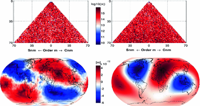
    Test of the rotated observation equations through closed-loop tests for \(\ell =T_i^e\) (left top/bottom panel) and \(\ell =T_{ij}^e\) (right top/bottom panel) and \(N=70\). The top panels depict the common digits of the input geopotential set and the recovered coefficients from the LS SHA. Common digits of the two sets \(P_1, P_2\) are determined by \(\log _{10}\left(\frac{|P_1|}{|P_1-P_2|}\right)\). The bottom panels display coefficient residuals in terms of height anomaly with \(\text{ RMS}=6.2\times 10^{-14}\) m (left) and \(\text{ RMS}=2.1\times 10^{-12}\) m (right)

References

  • Bettadpur SV (1992) Spherical harmonic synthesis and least squares computations in satellite gravity gradiometry. J Geod 66:261–271. doi:10.1007/BF02033186

    Google Scholar 

  • Bettadpur SV (1995) Hotine’s geopotential formulation: revisited. J Geod 69:135–142. doi:10.1007/BF00815482

    Google Scholar 

  • Bezděk A, Sebera J, Klokočník J, Kostelecký J (2012) Global gravity field models from the GPS positions of CHAMP, GRACE and GOCE satellites. In: Abbasi A, Giesen N (eds) EGU general assembly conference abstracts. EGU General Assembly Conference Abstracts, vol 14

  • Blais JA, Provins DA, Soofi MA (2006) Spherical harmonic transforms for discrete multiresolution applications. J Supercomput 38:173–187

    Article  Google Scholar 

  • Brockmann JM, Kargoll B, Krasbutter I, Schuh W-D, Wermuth M (2010) GOCE data analysis: from calibrated measurements to the global earth gravity field. Springer, Berlin

    Google Scholar 

  • Bruinsma S, Marty J, Balmino G, Biancale R, Foerste C, Abrikosov O, Neumayer H (2010) GOCE gravity field recovery by means of the direct numerical method. In: Presented at the ESA living planet symposium 2010, Bergen, Norway

  • Cruz J (1986) Ellipsoidal corrections to potential coefficients obtained from gravity anomaly data on the ellipsoid. The Ohio State University, Columbus, Ohio, Technical report 371

  • Cunningham LE (1970) On the computation of the spherical harmonic terms needed during the numerical integration of the orbital motion of an artificial satellite. Celest Mech 2:207–216

    Article  Google Scholar 

  • Ditmar P, Klees R, Kostenko F (2003) Fast and accurate computation of spherical harmonic coefficients from satellite gravity gradiometry data. J Geod 76:690–705. doi:10.1007/s00190-002-0298-x

    Article  Google Scholar 

  • ESA (1999) Gravity field and steady-state ocean circulation. Technical report, Reports for mission selection—the four Candidate Earth Explorer Core Missions, European Space Agency

  • Foerste C, Bruinsma S, Shako R, Marty J, Flechtner F, Abrikosov O, Dahle C, Lemoine J-M, Neumayer K, Biancale R, Barthelmes F, Knig R, Balmino G (2011) EIGEN-6—a new combined global gravity field model including GOCE data from the collaboration of GFZ-Potsdam and GRGS-Toulouse. Geophysical Research Abstracts, vol 13

  • Holmes SA, Featherstone WE (2002) A unified approach to the Clenshaw summation and the recursive computation of very high degree and order normalised associated Legendre functions. J Geod 76: 279–299

    Google Scholar 

  • Hotine M (1969) Mathematical Geodesy. ESSA, US Department of Commerce

  • Jekeli C (1981) The downward continuation to the Earth’s surface of truncated spherical and ellipsoidal harmonic series of the gravity and height anomalies. Technical Report 323, Ohio State Univestity.

  • Koop R, Stelpstra D (1989) On the computation of the gravitational potential and its first and second order derivatives. Manusc Geod 14:373–382

    Google Scholar 

  • Moritz H (2000) Geodetic reference system 1980. J Geod 74:128–162. doi:10.1007/s001900050278

    Article  Google Scholar 

  • Najafi-Alamdari M, Emadi S, Moghtased-Azar K (2006) The ellipsoidal correction to the Stokes kernel for precise geoid determination. J Geod 80:675–689. doi:10.1007/s00190-006-0050-z

    Google Scholar 

  • Pavlis NK (1988) Modeling and estimation of a low degree geopotential model from terrestrial gravity data. Technical Report 386, Ohio State University

  • Pavlis NK, Holmes SA, Kenyon SC, Factor J (2008) An Earth gravitational model to degree 2160: EGM2008. In: Presented at general assembly of the European Geosciences Union, Vienna, Austria

  • Petrovskaya M, Vershkov A (2006) Non-singular expressions for the gravity gradients in the local north-oriented and orbital reference frames. J Geod 80:117–127. doi:10.1007/s00190-006-0031-2

    Google Scholar 

  • Petrovskaya M, Vershkov A (2009) Construction of spherical harmonic series for the potential derivatives of arbitrary orders in the geocentric Earth-fixed reference frame. J Geod 84:165–178. doi:10.1007/s00190-009-0353-y

    Google Scholar 

  • Petrovskaya M, Vershkov A (2011) Basic equations for constructing geopotential models from the gravitational potential derivatives of the first and second orders in the terrestrial reference frame. J Geod 1–10: doi:10.1007/s00190-011-0535-2

  • Rapp R-H (1998) Past and future developments in geopotential modeling. In: Forsberg R, Feissel M, Dietrich R (eds) Geodesy on the move. Springer, Berlin, pp 58–78

    Chapter  Google Scholar 

  • Reed BG (1973) Application of kinematical geodesy for determining the short wave length components of the gravity field by satellite gradiometry. Technical Report 201, Ohio State Univestity

  • Sneeuw N (1994) Global spherical harmonic analysis by least-squares and numerical quadrature methods in historical perspective. Geophys J Int 118(3):707–716

    Article  Google Scholar 

  • The MathWorks Inc. (2008) MATLAB version R2008b, Natick, Massachusetts, USA

  • Tsoulis D (1999) Spherical harmonic computations with topographic/isostatic coefficients. Technical report, IAPG/FESG No. 3, Munich

Download references

Acknowledgments

This work was co-sponsored by ESA/PECS grant n. C98056 and by project CEDR LC506 of Ministry of Education of the Czech Republic. The authors thank to all reviewers and the editor, special thanks go to Dr. Pavel Ditmar for his detailed comments.

Author information

Authors and Affiliations

Authors

Corresponding author

Correspondence to Josef Sebera.

Appendices

Appendix A: Hotine’s harmonics and normalization factors

For the reader’s convenience, the relations between Hotine’s harmonics and the ordinary geopotential coefficients are listed. The original Hotine’s equations in Hotine (1969) are non-normalized and the similar functions in Bettadpur (1995); Petrovskaya and Vershkov (2009), (2011) use a different convention. Although in Hotine’s coefficients, the maximum order can formally exceed the degree of the input gravitational model, the true limit in order is given by the maximum degree/order of the gravitational model.

$$\begin{aligned}&\quad V_x: \\&{\left\{ \begin{array}{ll} \bar{C}_{n+1,0}^{x}&=\!\! \frac{1}{2} v_{+1}\bar{C}_{n,1}\\ \bar{S}_{n+1,0}^{x}&\!\! = 0 \\ \end{array}\right.} \\&{\left\{ \begin{array}{ll} \bar{C}_{n+1,1}^{x}&\!\!= -v_{-1}\bar{C}_{n,0} + \frac{1}{2}v_{+1}\bar{C}_{n,2} \\ \bar{S}_{n+1,1}^{x}&\!\!= +\frac{1}{2} v_{+1}\bar{S}_{n,2}\\ \end{array}\right.} \\&{\left\{ \begin{array}{ll} \bar{C}_{n+1,m}^{x}&\!\!= -\frac{1}{2} v_{-1}\bar{C}_{n,m-1} + \frac{1}{2}v_{+1} \bar{C}_{n,m+1}\\ \bar{S}_{n+1,m}^{x}&\!\!= -\frac{1}{2} v_{-1}\bar{S}_{n,m-1} + \frac{1}{2}v_{+1} \bar{S}_{n,m+1}\\ \end{array}\right.}\\&\quad V_y: \\&{\left\{ \begin{array}{ll} \bar{C}_{n+1,0}^{y}&\!\!= \frac{1}{2} v_{+1}\bar{S}_{n,1}\\ \bar{S}_{n+1,0}^{y}&\!\!= 0 \\ \end{array}\right.} \\&{\left\{ \begin{array}{ll} \bar{C}_{n+1,1}^{y}&\!\!= +\frac{1}{2} v_{+1}\bar{S}_{n,2} \\ \bar{S}_{n+1,1}^{y}&\!\! = -v_{-1}\bar{C}_{n,0} - \frac{1}{2}v_{+1}\bar{C}_{n,2}\\ \end{array}\right.} \\&{\left\{ \begin{array}{ll} \bar{C}_{n+1,m}^{y}&\!\! = \frac{1}{2} v_{-1}\bar{S}_{n,m-1} + \frac{1}{2}v_{+1} \bar{S}_{n,m+1}\\ \bar{S}_{n+1,m}^{y}&\!\!= -\frac{1}{2} v_{-1}\bar{C}_{n,m-1} - \frac{1}{2}v_{+1} \bar{C}_{n,m+1}\\ \end{array}\right.}\\&\quad V_z: \\&{\left\{ \begin{array}{ll} \bar{C}_{n+1,0}^{z}&\!\!= -v_0 \bar{C}_{n,0}\\ \bar{S}_{n+1,0}^{z}&\!\!= 0 \\ \end{array}\right.} \\&{\left\{ \begin{array}{ll} \bar{C}_{n+1,1}^{z}&\!\!= -v_0 \bar{C}_{n,1} \\ \bar{S}_{n+1,1}^{z}&\!\!= -v_0 \bar{S}_{n,1} \\ \end{array}\right.} \\&{\left\{ \begin{array}{ll} \bar{C}_{n+1,m}^{z}&\!\!= -v_0 \bar{C}_{n,m} \\ \bar{S}_{n+1,m}^{z}&\!\!= -v_0 \bar{S}_{n,m} \\ \end{array}\right.} \\&\quad V_{xx}:\\&{\left\{ \begin{array}{ll} \bar{C}_{n+2,0}^{xx}&\!\!= -\frac{1}{2} t_0\bar{C}_{n,0} + \frac{1}{4}t_{+2} \bar{C}_{n,2} \\ \bar{S}_{n+2,0}^{xx}&\!\!= 0 \\ \end{array}\right.} \\&{\left\{ \begin{array}{ll} \bar{C}_{n+2,1}^{xx}&\!\!= -\frac{3}{4} t_0\bar{C}_{n,1} + \frac{1}{4}t_{+2} \bar{C}_{n,3} \\ \bar{S}_{n+2,1}^{xx}&\!\!= -\frac{1}{4} t_0\bar{S}_{n,1} + \frac{1}{4}t_{+2} \bar{S}_{n,3} \\ \end{array}\right.} \\&{\left\{ \begin{array}{ll} \bar{C}_{n+2,2}^{xx}&\!\! = \frac{1}{4} t_{-2}\bar{C}_{n,0} - \frac{1}{2}t_0 \bar{C}_{n,2} + \frac{1}{4}t_{+2} \bar{C}_{n,4} \\ \bar{S}_{n+2,2}^{xx}&\!\!= - \frac{1}{2}t_0 \bar{S}_{n,2} + \frac{1}{4}t_{+2} \bar{S}_{n,4} \end{array}\right.} \\&{\left\{ \begin{array}{ll} \bar{C}_{n+2,m}^{xx}&\!\!= \frac{1}{4} t_{-2}\bar{C}_{n,m-2} - \frac{1}{2}t_0 \bar{C}_{n,m} + \frac{1}{4}t_{+2} \bar{C}_{n,m+2} \\ \bar{S}_{n+2,m}^{xx}&\!\!= \frac{1}{4} t_{-2}\bar{S}_{n,m-2} - \frac{1}{2}t_0 \bar{S}_{n,m} + \frac{1}{4}t_{+2} \bar{S}_{n,m+2} \\ \end{array}\right.}\\&\quad V_{yy}:\\&{\left\{ \begin{array}{ll} \bar{C}_{n+2,0}^{yy}&\!\!= -\frac{1}{2} t_0\bar{C}_{n,0} - \frac{1}{4}t_{+2} \bar{C}_{n,2} \\ \bar{S}_{n+2,0}^{yy}&\!\!= 0 \\ \end{array}\right.} \\&{\left\{ \begin{array}{ll} \bar{C}_{n+2,1}^{yy}&\!\!= -\frac{1}{4} t_0\bar{C}_{n,1} - \frac{1}{4}t_{+2} \bar{C}_{n,3} \\ \bar{S}_{n+2,1}^{yy}&\!\!= -\frac{3}{4} t_0\bar{S}_{n,1} - \frac{1}{4}t_{+2} \bar{S}_{n,3} \\ \end{array}\right.} \\&{\left\{ \begin{array}{ll} \bar{C}_{n+2,2}^{yy}&\!\!= -\frac{1}{4} t_{-2}\bar{C}_{n,0} - \frac{1}{2}t_0 \bar{C}_{n,2} - \frac{1}{4}t_{+2} \bar{C}_{n,4} \\ \bar{S}_{n+2,2}^{yy}&\!\!= - \frac{1}{2}t_0 \bar{S}_{n,2} - \frac{1}{4}t_{+2} \bar{S}_{n,4} \end{array}\right.} \\&{\left\{ \begin{array}{ll} \bar{C}_{n+2,m}^{xx}&\!\!= \frac{1}{4} t_{-2}\bar{C}_{n,m-2} - \frac{1}{2}t_0 \bar{C}_{n,m} + \frac{1}{4}t_{+2} \bar{C}_{n,m+2} \\ \bar{S}_{n+2,m}^{xx}&\!\!= \frac{1}{4} t_{-2}\bar{S}_{n,m-2} - \frac{1}{2}t_0 \bar{S}_{n,m} + \frac{1}{4}t_{+2} \bar{S}_{n,m+2} \\ \end{array}\right.}\\&\quad V_{zz}:\\&{\left\{ \begin{array}{ll} \bar{C}_{n+2,0}^{zz}&\!\!= t_0\bar{C}_{n,0} \\ \bar{S}_{n+2,0}^{zz}&\!\!= 0 \\ \end{array}\right.} \\&{\left\{ \begin{array}{ll} \bar{C}_{n+2,1}^{zz}&\!\!= t_0\bar{C}_{n,1} \\ \bar{S}_{n+2,1}^{zz}&\!\!= t_0\bar{S}_{n,1} \\ \end{array}\right.} \\&{\left\{ \begin{array}{ll} \bar{C}_{n+2,2}^{zz}&\!\!= t_0\bar{C}_{n,2} \\ \bar{S}_{n+2,2}^{zz}&\!\!= t_0\bar{S}_{n,2} \end{array}\right.} \\&{\left\{ \begin{array}{ll} \bar{C}_{n+2,m}^{zz}&\!\!= t_0\bar{C}_{n,m}\\ \bar{S}_{n+2,m}^{zz}&\!\!= t_0\bar{S}_{n,m} \\ \end{array}\right.}\\&\quad V_{xy}:\\&{\left\{ \begin{array}{ll} \bar{C}_{n+2,0}^{xy}&\!\!= \frac{1}{4}t_{+2} \bar{S}_{n,2} \\ \bar{S}_{n+2,0}^{xy}&\!\!= 0 \\ \end{array}\right.} \\&{\left\{ \begin{array}{ll} \bar{C}_{n+2,1}^{xy}&\!\!= -\frac{1}{4} t_0\bar{S}_{n,1} + \frac{1}{4}t_{+2} \bar{S}_{n,3} \\ \bar{S}_{n+2,1}^{xy}&\!\!= -\frac{1}{4} t_0\bar{C}_{n,1} - \frac{1}{4}t_{+2} \bar{C}_{n,3} \\ \end{array}\right.} \\&{\left\{ \begin{array}{ll} \bar{C}_{n+2,2}^{xy}&\!\!= \frac{1}{4} t_{+2}\bar{S}_{n,4} \\ \bar{S}_{n+2,2}^{xy}&\!\!= \frac{1}{2}t_{-2} \bar{C}_{n,0} - \frac{1}{4}t_{+2} \bar{C}_{n,4} \end{array}\right.} \\&{\left\{ \begin{array}{ll} \bar{C}_{n+2,m}^{xy}&\!\!= -\frac{1}{4}t_{-2} \bar{S}_{n,m-2} + \frac{1}{4}t_{+2} \bar{S}_{n,m+2} \\ \bar{S}_{n+2,m}^{xy}&\!\!= \frac{1}{4}t_{-2} \bar{C}_{n,m-2} - \frac{1}{4}t_{+2} \bar{C}_{n,m+2} \\ \end{array}\right.}\\&\quad V_{xz}:\\&{\left\{ \begin{array}{ll} \bar{C}_{n+2,0}^{xz}&\!\!= -\frac{1}{2}t_{+1} \bar{C}_{n,1} \\ \bar{S}_{n+2,0}^{xz}&\!\!= 0 \\ \end{array}\right.} \\&{\left\{ \begin{array}{ll} \bar{C}_{n+2,1}^{xz}&\!\!= t_{-1}\bar{C}_{n,0} - \frac{1}{2}t_{+1} \bar{C}_{n,2}\\ \bar{S}_{n+2,1}^{xz}&\!\!= -\frac{1}{2} t_{+1}\bar{S}_{n,2}\\ \end{array}\right.} \\&{\left\{ \begin{array}{ll} \bar{C}_{n+2,m}^{xz}&\!\!= \frac{1}{2} t_{-1}\bar{C}_{n,m-1} -\frac{1}{2} t_{+1}\bar{C}_{n,m+1} \\ \bar{S}_{n+2,m}^{xz}&\!\!= \frac{1}{2} t_{-1}\bar{S}_{n,m-1} -\frac{1}{2} t_{+1}\bar{S}_{n,m+1} \\ \end{array}\right.}\\&\quad V_{yz}:\\&{\left\{ \begin{array}{ll} \bar{C}_{n+2,0}^{yz}&\!\!= -\frac{1}{2}t_{+1} \bar{S}_{n,1} \\ \bar{S}_{n+2,0}^{yz}&\!\! = 0 \\ \end{array}\right.} \\&{\left\{ \begin{array}{ll} \bar{C}_{n+2,1}^{yz}&\!\!= -\frac{1}{2} t_{+1}\bar{S}_{n,2} \\ \bar{S}_{n+2,1}^{yz}&\!\!= t_{-1}\bar{C}_{n,0} + \frac{1}{2}t_{+1} \bar{C}_{n,2} \\ \end{array}\right.} \\&{\left\{ \begin{array}{ll} \bar{C}_{n+2,m}^{yz}&\!\! = -\frac{1}{2} t_{-1}\bar{S}_{n,m-1} -\frac{1}{2} t_{+1}\bar{S}_{n,m+1} \\ \bar{S}_{n+2,m}^{yz}&\!\!= \frac{1}{2} t_{-1}\bar{C}_{n,m-1} +\frac{1}{2}t_{+1}\bar{C}_{n,m+1} \\ \end{array}\right.} \end{aligned}$$

Normalized Hotine’s factors for the acceleration vector read (use of \(v\) implicates they refer to a vector):

$$\begin{aligned} v_0&= \sqrt{\frac{(2n+1)(n+m+1)(n-m+1)}{2n+3}}, \\ v_{-1}&= a \sqrt{\frac{(2n+1)(n+m+1)(n+m)}{2n+3}}\\&\text{ with}\,\, a =\frac{1}{\sqrt{2}}\,\, {\text{ for}}\,\, m=1, a=1 \,\,\text{ otherwise} \\ v_{+1}&= a \sqrt{\frac{(2n+1)(n-m+1)(n-m)}{2n+3}}\\&\text{ with}\,\, a=\sqrt{2} \,\,\text{ for}\,\, m=0,a=1\,\,\text{ otherwise} \end{aligned}$$

and similarly for the components of the Eötvös tensor (use of \(t\) implicates they refer to a tensor):

$$\begin{aligned} t_0 \!&= \!\sqrt{\frac{(2n\!+\!1)(n\!+\!m\!+\!2)(n\!+\!m\!+\!1)(n\!-\!m\!+\!2)(n\!-\!m\!+\!1)}{2n\!+\!5}}, \\ t_{\!-\!1} \!&= \!a\sqrt{\frac{(2n\!+\!1)(n\!+\!m\!+\!2)(n\!+\!m\!+\!1)(n\!+\!m)(n\!-\!m\!+\!2)}{2n\!+\!5}} \\&\text{ with}\,\,a=\frac{1}{\sqrt{2}} \,\,\text{ for}\,\, m=1,a=1 \,\,\text{ otherwise}\\ t_{\!+\!1} \!&= \!a\sqrt{\frac{(2n\!+\!1)(n\!+\!m\!+\!2)(n\!-\!m\!+\!1)(n\!-\!m)(n\!-\!m\!+\!2)}{2n\!+\!5}}\\&\text{ with}\,\, a=\sqrt{2} \,\,\text{ for}\,\, m=0,a=1\,\, \text{ otherwise} \\ t_{\!+\!2} \!&= \!a \sqrt{\frac{(2n\!+\!1)(n\!+\!m\!+\!2)(n\!+\!m\!+\!1)(n\!+\!m)(n\!-\!m\!+\!2)}{2n\!+\!5}}\\&\text{ with}\,\, a=\sqrt{2} \,\,\text{ for}\,\, m=0,a=1 \,\,\text{ otherwise} \\ t_{\!-\!2} \!&= \!a\sqrt{\frac{(2n\!+\!1)(n\!+\!m\!+\!2)(n\!+\!m\!+\!1)(n\!+\!m)(n\!-\!m\!-\!1)}{2n\!+\!5}}\\&\text{ with}\,\, a=\sqrt{2} \,\,\text{ for}\,\, m=2,a=1 \,\,\text{ otherwise}. \end{aligned}$$

The better overview of the exceptions defined by multiplier \(a\) is shown in Fig. 5, where the exceptions are red points. The exceptions hold for the whole order.

Fig. 5
figure 5

Use of the multiplier \(a\) in \(v_{+1},v_{-1},t_{+1},t_{-1},t_{+2},t_{-2}\) (in red) for degree 4

Appendix B: Rotational matrices

With the ordinary rotational matrix \(R\)

$$\begin{aligned} R= \begin{pmatrix} r_{11}&\quad r_{12}&\quad r_{13} \\ r_{21}&\quad r_{22}&\quad r_{23} \\ r_{31}&\quad r_{32}&\quad r_{33} \end{pmatrix}, \end{aligned}$$

and the transformation law for tensors \(V_{ij}=R V_{ij}^{^{\prime }} R^\mathrm{T} \) we get the matrix \(S\)

$$\begin{aligned}&S = \begin{pmatrix} s_{1}^{xx}&\quad s_{2}^{xx}&\quad s_{3}^{xx}&\quad s_{4}^{xx}&\quad s_{5}^{xx}&\quad s_{6}^{xx} \\ s_{1}^{yy}&\quad s_{2}^{yy}&\quad s_{3}^{yy}&\quad s_{4}^{yy}&\quad s_{5}^{yy}&\quad s_{6}^{yy} \\ s_{1}^{zz}&\quad s_{2}^{zz}&\quad s_{3}^{zz}&\quad s_{4}^{zz}&\quad s_{5}^{zz}&\quad s_{6}^{zz} \\ s_{1}^{xy}&\quad s_{2}^{xy}&\quad s_{3}^{xy}&\quad s_{4}^{xy}&\quad s_{5}^{xy}&\quad s_{6}^{xy} \\ s_{1}^{xz}&\quad s_{2}^{xz}&\quad s_{3}^{xz}&\quad s_{4}^{xz}&\quad s_{5}^{xz}&\quad s_{6}^{xz} \\ s_{1}^{yz}&\quad s_{2}^{yz}&\quad s_{3}^{yz}&\quad s_{4}^{yz}&\quad s_{5}^{yz}&\quad s_{6}^{yz} \end{pmatrix} =\\&\quad \begin{pmatrix} r_{13}^2&\, r_{12}^2&\, r_{11}^2&\, 2r_{11}r_{12}&\, 2r_{13}r_{11}&\, 2r_{13}r_{12} \\ r_{23}^2&\, r_{22}^2&\, r_{21}^2&\, 2r_{21}r_{22}&\, 2r_{21}r_{23}&\, 2r_{22}r_{23} \\ r_{33}^2&\, r_{32}^2&\, r_{31}^2&\, 2r_{31}r_{32}&\, 2r_{31}r_{33}&\, 2r_{32}r_{33} \\ r_{13}r_{23}&\, r_{12}r_{22}&\, r_{11}r_{21}&\, (r_{12}r_{21}+r_{11}r_{22})&\, (r_{13}r_{21} +r_{11}r_{23})&\, (r_{13}r_{22} + r_{12}r_{23}) \\ r_{13}r_{33}&\, r_{12}r_{32}&\, r_{11}r_{31}&\, (r_{12}r_{31}+r_{11}r_{32})&\, (r_{13}r_{31} +r_{11}r_{33})&\, (r_{13}r_{32} + r_{12}r_{33}) \\ r_{23}r_{33}&\, r_{22}r_{32}&\, r_{21}r_{31}&\, (r_{22}r_{31} +r_{21}r_{32})&\, (r_{23}r_{31} +r_{21}r_{33})&\, (r_{23}r_{32} + r_{22}r_{33}) \end{pmatrix}. \end{aligned}$$

For example, transfer from the EFF into the spherical LNOF is provided by rotational sequence:

$$\begin{aligned} R\!=\!R_y(-\theta )R_z(\lambda - \pi )\!=\! \begin{pmatrix} \cos \theta&\quad 0&\quad \sin \theta \\ 0&\quad 1&\quad 0 \\ -\sin \theta&\quad 0&\cos \theta \\ \end{pmatrix} \begin{pmatrix} \cos (\lambda - \pi )&\quad \sin (\lambda - \pi )&0 \\ -\sin (\lambda - \pi )&\quad \cos (\lambda - \pi )&0 \\ 0&0&1 \end{pmatrix}. \end{aligned}$$

Adding one more rotation around \(y\) axis for a difference between latitudes \(\alpha ={\varphi }_g-\varphi _s=\theta -\vartheta \) we move from the spherical into the ellipsoidal LNOF:

$$\begin{aligned} R=R_y(\alpha )R_y(-\theta )R_z(\lambda - \pi ). \end{aligned}$$

Appendix C: Matlab codes of the design matrix for \(V_i\) and \(V_{ij}\)

The input matrix with the ALFs has to keep the triangular convention from Fig. 5 (order in columns, degree in rows with \(\bar{P}_{0,0}\) at upper left corner). For the acceleration vector, this matrix must be generated up to \(N+1\), whereas for the Eötvös tensor up to \(N+2\). The routines evaluate all degree/order functions \(v_0,v_{\pm 1},t_0,t_{\pm 1},t_{\pm 2}\) each time the function is called. This is only due to the compactness of the code presented. As these d/o functions do not depend on (\(r,\theta ,\lambda \)), they can be computed before the routines “tiA”, “tijA” are called.

1.1 C.1 The design matrix for the acceleration vector

figure a1

1.2 C.2 The design matrix for the Eötvös tensor

figure a2
figure a3

Rights and permissions

Reprints and permissions

About this article

Cite this article

Sebera, J., Wagner, C.A., Bezděk, A. et al. Short guide to direct gravitational field modelling with Hotine’s equations. J Geod 87, 223–238 (2013). https://doi.org/10.1007/s00190-012-0591-2

Download citation

  • Received:

  • Accepted:

  • Published:

  • Issue Date:

  • DOI: https://doi.org/10.1007/s00190-012-0591-2

Keywords

Navigation