
Abstract
We study circle-valued maps and consider the persistence of the homology of their fibers. The outcome is a finite collection of computable invariants which answer the basic questions on persistence and in addition encode the topology of the source space and its relevant subspaces. Unlike persistence of real-valued maps, circle-valued maps enjoy a different class of invariants called Jordan cells in addition to bar codes. We establish a relation between the homology of the source space and of its relevant subspaces with these invariants and provide a new algorithm to compute these invariants from an input matrix that encodes a circle-valued map on an input simplicial complex.
1 Introduction
Data analysis provides many scenarios where one ends up with a nice space, most often a simplicial complex, a smooth manifold, or a stratified space equipped with a real-valued or a circle-valued map. The persistence theory, introduced in [14], provides a useful tool for analyzing real-valued maps with the help of homology. A similar theory for circle-valued maps has not yet been developed in the literature. The work in [9] introduces the concept of circle-valued maps in the context of persistence by deriving a circle-valued map for given data by using the existing persistence theory. In contrast, we develop a persistence theory for circle-valued maps.
One place where circle-valued maps appear naturally is the area of dynamics of vector fields. Many dynamics are described by vector fields which admit a minimizing action (in mathematical terms a Lyapunov closed one form). Such actions can be interpreted as 1-cocycles which are intimately connected to circle-valued maps as shown in [3]. Consequently, a notion of persistence for circle-valued maps also provides a notion of persistence for 1-cocycles which appear in some data analysis problems [20, 21]. In summary, persistence theory for circle-valued maps promises to play the role for some vector fields as does the standard persistence theory for the scalar fields [6, 7, 14, 22].
One of the main concepts of the persistence theory is the notion of bar codes [22]—invariants that characterize a real-valued map at the homology level. The angle (circle) valued maps, when characterized at homology level, require a new invariant called Jordan cells in addition to the refinement of the bar codes into four types.
The standard persistence [14, 22] which we refer as sublevel persistence deals with the change in the homology of the sublevel sets which cannot make sense for a circle-valued map. However, the change in the homology of the level sets can be considered for both real- and circle-valued maps. The notion of persistence, when considered for the level sets of a real-valued map [10] is referred here as level persistence. It refines the sublevel persistence. The zigzag persistence introduced in [4] provides complete invariants (bar codes) for level persistence of (tame) real-valued maps. They are defined by using representation theory for linear quivers.
The change in homology of the level sets of a (tame) circle-valued map is more complicated because of the return of the level to itself when one goes along the circle. It turns out that representation theory of cyclic quivers provides the complete invariants for persistence in the homology of the level sets of the circle-valued maps. This notion of persistence is called here the persistence for circle-valued maps and its invariants, bar codes and Jordan cells are shown to be effectively computable.
Our results include a derivation of the homology for the source space and its relevant subspaces in terms of the invariants (Theorems 3.1 and 3.2). The result also applies to real-valued maps as they are special cases of the circle-valued maps. This leads to a result (Corollary 3.4) which to our knowledge has not yet appeared in the literature.Footnote 1 A number of other topological results which cannot be derived from any of the previously defined persistence theories are described in [2] providing additional motivation for this work.
After developing the results on invariants, we propose a new algorithm to compute the bar codes and Jordan cells. For a simplicial complex, the entire computation can be done by manipulating the original matrix that encodes the input complex and the map. The algorithm first builds a block matrix from the original incidence matrix which encodes linear maps induced in homology among regular and critical level sets, more precisely the quiver representations \(\rho _r\) described in Sect. 4. Next, it iteratively reduces this new matrix eliminating and hence computing the bar codes. The resulting matrix which is invertible can be further processed to Jordan canonical form [12] providing Jordan cells. The algorithm for zigzag persistence [4] when applied to what we refer in Sect. 3 as the infinite cyclic covering map \(\tilde{f}\) can compute bar codes but not Jordan cells. In contrast, our method can compute the bar codes and Jordan cells simultaneously by manipulating matrices and can also be used as an alternative to compute the bar codes in zig-zag persistence.
Notations. We list here some of the notations that are used throughout.
-
For \(r\)th homology group of a topological space X under an a priori fixed field \(\kappa \), we write \(H_r(X)\) instead of \(H_r(X;\kappa )\).
-
For a map \(f:X\rightarrow Y\) and \(K\subseteq Y\) we write \(X_K:= f^{-1}(K)\).
-
We use \(\mathbb Z _{\ge 0}\) and \(\mathbb Z _{>0}\) for non-negative and positive integers respectively.
-
In our exposition, we need to use open, semi-open, and closed intervals denoted as \((a,b)\), \((a,b]\) or \([a,b)\), and \([a,b]\) respectively. To denote an interval, in general, we use the notation \(\{a,b\}\) where “{” stands for either “[” or “(”.
-
For a linear map \(\alpha : V\rightarrow W\) between two vector spaces we write:
$$\begin{aligned}&\ker \alpha :=\big \{v\in V \mid \alpha (v)=0\big \},\\&\mathrm img \ \alpha := \big \{w\in \alpha (V)\subseteq W\big \},\\&\mathrm coker\ \alpha := W/\alpha (V). \end{aligned}$$ -
A matrix A is said to be in column echelon form if all zero columns, if any, are on the right to nonzero ones and the leading entry (the first nonzero number from below) of a nonzero column is always strictly below of the leading entry of the next column. Similarly, A is said to be in row echelon form if all zero rows, if any, are below nonzero ones and the leading entry (the first nonzero number from the right) of a nonzero row is always strictly to the right of the leading entry of the row below it. If A is an \(m\times n\) matrix (m rows and n columns), there exist an invertible \(n\times n\) matrix \(R(A)\) and an invertible \(m\times m\) matrix \(L(A)\) so that \(A\cdot R(A)\) is in column echelon form and \(L(A)\cdot A\) is in row echelon form. Algorithms for deriving the column and row echelon form can be found in standard books on linear algebra.
2 Definitions and Background
We begin with the technical definition of tameness of a map.
For a continuous map \(f: X\rightarrow Y\) between two topological spaces X and Y, let \(X_U= f^{-1}(U)\) for \(U\subseteq Y\). When \(U=y\) is a single point, the set \(X_y\) is called a fiber over y and is also commonly known as the level set of y. We call the continuous map \(f:X\rightarrow Y\) good if every \(y\in Y\) has a contractible neighborhood U so that the inclusion \(X_y\rightarrow X_U\) is a homotopy equivalence. The continuous map \(f:X\rightarrow Y\) is a fibration if each \(y\in Y\) has a neighborhood U so that the maps \(f: X_U \rightarrow U\) and \(pr: X_y\times U\rightarrow U\) are fiber wise homotopy equivalent. This means that there exist continuous maps \(l:X_U\rightarrow X_y\times U\) with \(pr|_U \cdot l|_U = f|_U\) which, when restricted to the fiber for any \(z\in U\), are homotopy equivalences. In particular, f is good.
Definition 2.1
A proper continuous map \(f:X\rightarrow Y\) is tame if it is good, and for some discrete closed subset \(S\subset Y\), the restriction \(f: X\setminus f^{-1}(S) \rightarrow Y \setminus S\) is a fibration. The points in \(S\subset Y\) which prevent f to be a fibration are called critical values.
If \(Y= \mathbb R \) and X is compact or \(Y= \mathbb{S }^1,\) Footnote 2 then the set of critical values is finite, say \(s_1 < s_2 < \cdots s_k.\) The fibers above them, \(X_{s_i},\) are referred to as singular fibers. All other fibers are called regular. In the case of \(\mathbb{S }^1\), \(s_i\) can be taken as angles and we can assume that \(0< s_i \le 2\pi .\) Clearly, for the open interval \((s_{i-1},s_i)\) the map \(f: f^{-1}(s_{i-1}, s_{i}) \rightarrow (s_{i-1}, s_{i})\) is a fibration which implies that all fibers over angles in \((s_{i-1}, s_i)\) are homotopy equivalent with a fixed regular fiber, say \(X_{t_i}\), with \(t_i\in (s_{i-1}, s_i)\).

In particular, there exist maps \(a_i: X_{t_i}\rightarrow X_{s_i}\) and \(b_i: X_{t_{i+1}}\rightarrow X_{s_{i}}\), unique up to homotopy defined as follows: If \(t_i\) and \(t_{i+1}\) are contained in \(U_i \subset Y\) where the inclusion \(X_{s_i} \subset X_{U_i}\) is a homotopy equivalence with a homotopy inverse \(r_i: X_{U_i} \rightarrow X_{s_i},\) then \(a_i\) and \(b_i\) are the restrictions of \(r_i\) to \(X_{t_i}\) and \(X_{t_{i+1}}\) respectively. If not, in view of the tameness of f, one can find \(t^{\prime }_i\) and \( t^{\prime }_{i+1}\) in \(U_i\) so that \(X_{t_i}\) and \(X_{t_{i+1}}\) are homotopy equivalent to \(X_{t^{\prime }_i}\) and \(X_{t^{\prime }_{i+1}}\) respectively and compose the restrictions of \(r_i\) with these homotopy equivalences.
These maps determine homotopically \(f:X\rightarrow Y,\) when \(Y= \mathbb R \) or \(\mathbb{S ^1}\). For simplicity in writing, when \(Y= \mathbb R \) we put \(t_{k+1}\in (s_k, \infty )\) and \(t_1\in (-\infty , s_1)\) and when \(Y=\mathbb{S }^1\) we put \(t_{k+1}=t_1 \in (s_k, s_1+2\pi ).\) All scalar or circle-valued simplicial maps on a simplicial complex, and all smooth maps with generic isolated critical points on a smooth manifold or stratified space are tame. In particular, Morse maps are tame.
2.1 Persistence and Invariants for Real-Valued Maps
Since our goal is to extend the notion of persistence from real-valued maps to circle-valued maps, we first summarize the questions that the persistence answers when applied to real-valued maps, and then develop a notion of persistence for circle-valued maps which can answer similar questions and more. We fix a field \(\kappa \) and write \(H_r(X)\) to denote the homology vector space of X in dimension r with coefficients in a field \(\kappa .\)
Sublevel persistence. The persistent homology introduced in [14] and further developed in [22] is concerned with the following questions:
-
Q1.
Does the class \(x\in H_r(X_{(-\infty ,t]})\) originate in \(H_r(X_{(-\infty ,t^{\prime \prime }]})\) for \(t^{\prime \prime }< t\)? Does the class \(x\in H_r(X_{(-\infty ,t]})\) vanish in \(H_r(X_{(-\infty ,t^{\prime }]})\) for \(t<t^{\prime }\)?
-
Q2.
What are the smallest \(t^{\prime }\) and largest \(t^{\prime \prime }\) such that this happens?
This information is contained in the inclusion induced linear maps \(H_r(X_{(-\infty ,t]}) \rightarrow H_r(X_{(-\infty ,t^{\prime }]})\) where \(t^{\prime }\ge t\) and is known as persistence. Since the involved subspaces are sublevel sets, we refer to this persistence as sublevel persistence. When f is tame, the persistence for each \(r= 0, 1,\ldots , \dim X,\) is determined by a finite collection of invariants referred to as bar codes [22]. For sublevel persistence the bar codes are a collection of closed intervals of the form \([s,s^{\prime }] \) or \([s,\infty )\) with \(s, s^{\prime }\) being the critical values of f. From these bar codes one can derive the Betti numbers of \(X_{(-\infty , a]},\) the dimension of \(\mathrm {img}(H_r (X_{(-\infty ,t]}) \rightarrow H_r(X_{(-\infty ,t^{\prime }]}))\) and get the answers to questions Q1 and Q2. For example, the number of r-bar codes which contain the interval \([a,b]\) is the dimension of \(\mathrm {img}(H_r (X_{(-\infty ,a]}) \rightarrow H_r(X_{(-\infty ,b]})).\) The number of r-bar codes which identify to the interval \([a,b]\) is the maximal number of linearly independent homology classes born exactly in \(X_{(-\infty ,a]}\) but not before and die exactly in \(H_r(X_{-\infty , b]})\) but not before.
Level persistence. Instead of sublevels, if we use levels, we obtain what we call level persistence. The level persistence was first considered in [10] but was better understood computationally when the zig-zag persistence was introduced in [4]. Level persistence is concerned with the homology of the fibers \(H_r(X_t)\) and addresses questions of the following type.
-
Q1.
Does the image of \(x\in H_r(X_t)\) vanish in \(H_r(X_{[t,t^{\prime }]}),\) where \(t^{\prime }>t\) or in \(H_r (X_{[t^{\prime \prime }, t]}),\) where \(t^{\prime \prime }<t\)?
-
Q2.
Can x be detected in \(H_r(X_{t^{\prime }})\) where \(t^{\prime }>t\) or in \(H_r(X_{t^{\prime \prime }})\) where \( t^{\prime \prime } <t\)? The precise meaning of detection is explained below.
-
Q3.
What are the smallest \(t^{\prime }\) and the largest \(t^{\prime \prime }\) for the answers to Q1 and Q2 to be affirmative?
To answer such questions one needs information about the following inclusion induced linear maps:
The level persistence is the information provided by this collection of vector spaces and linear maps for all \(t,t^{\prime }.\)
We say that \(x\in H_r(X_t)\) is dead in \(H_r(X_{[t,t^{\prime }]}), \ t^{\prime }>t\), if its image by \(H_r(X_t)\rightarrow H_r(X_{[t, t^{\prime }]})\) vanishes. Similarly, x is dead in \(H_r(X_{[t^{\prime \prime },t]}), \ t^{\prime \prime }<t\), if its image by \(H_r(X_t)\rightarrow H_r(X _{[t^{\prime \prime }, t]})\) vanishes.
We say that \(x\in H_r(X_t)\) is detected in \(H_r (X_{t^{\prime }}),\ t^{\prime }>t\) (resp. \(t^{\prime \prime }<t\)), if its image in \(H_r(X_{[t,t^{\prime }]})\) (resp. in \(H_r(X_{[t^{\prime \prime },t]}\)) is nonzero and is contained in the image of \(H_r(X_{t^{\prime }})\rightarrow H_r(X_{[t, t^{\prime }]})\) (resp. \(H_r(X_{t^{\prime \prime }})\rightarrow H_r(X_{[t^{\prime \prime }, t]})\)). In Fig. 1, the class consisting of the sum of two circles at level t is not detected on the right, but is detected at all levels on the left up to (but not including) the level \(t^{\prime }\). In case of a tame map the collection of the vector spaces and linear maps is determined up to coherent isomorphisms by a collection of invariants called bar codes for level persistence which are intervals of the form \([s, s^{\prime }], (s,s^{\prime }), (s,s^{\prime }], [s,s^{\prime })\) with \(s, s^{\prime }\) critical values as opposed to the bar codes for sublevel persistence which are intervals of the form \({[s,s^{\prime }], [s,\infty )}\) with \(s,s^{\prime } \) critical values. These bar codes are called invariants because two tame maps \(f:X\rightarrow \mathbb R \) and \(g:Y\rightarrow \mathbb R \) which are fiber wise homotopy equivalent have the same associated bar codes. In the case of level persistence the open end of an interval signifies the death of a homology class at that end (left or right) whereas a closed end signifies that a homology class cannot be detected beyond this level (left or right). In the case of the sublevel persistence the left end signifies birth while the right death. Level persistence provides considerably more information than the sublevel persistence. The bar codes of the sublevel persistence can be recovered from the ones of level persistence. Precisely a level bar code \([s,s^{\prime }]\) gives a sublevel bar code \([s,\infty )\) and a level bar code \([s,s^{\prime })\) gives a sublevel bar code \([s, s^{\prime }];\) the sublevel persistence does not see any of the level bar codes \((s, s^{\prime })\) or \((s,s^{\prime }]\). It turns out that the bar codes of the level persistence can also be recovered from the bar codes of the sublevel persistence of f and additional maps canonically associated to f.

Bar codes for level and sublevel persistence
In Fig. 1, we indicate the bar codes both for sublevel and level persistenceFootnote 3 for some simple map \(f:X \rightarrow \mathbb R \) in order to illustrate their differences. The space X is a tube open on one end and f is the height function laid horizontally.
3 Persistence for Circle-Valued Maps
Let \(f:X\rightarrow \mathbb{S }^1\) be a circle-valued map. The sublevel persistence for such a map cannot be defined since circularity in values prevents defining sublevels. Even level persistence cannot be defined as per se since the intervals may repeat over values. To overcome this difficulty we associate the infinite cyclic covering map \(\tilde{f}:\tilde{X}\rightarrow \mathbb R \) for f. It is defined by the commutative diagram:

The map \(p: \mathbb R \rightarrow \mathbb S ^1\) is the universal covering of the circle (the map which assigns to the number \(t\in \mathbb R \) the angle \(\theta = t ({\mathrm{{mod}}}~2\pi )\) and \(\psi \) is the pull back of p by the map f which is an infinite cyclic covering. Notice that if \(p(t)=\theta \) then \( \tilde{X}_t \) and \(X_\theta \) are identified by \(\psi .\) If \(x\in H_r(X_\theta )= H_r(\tilde{X}_t), \ p(t)=\theta ,\) the questions Q1, Q2, Q3 for f and X can be formulated in terms of the level persistence for \(\tilde{f}\) and \(\tilde{X}\).
Suppose that \(x\in H_r(\tilde{X}_t)= H_r(X_\theta ) \) is detected in \(H_r(\tilde{X}_{t^{\prime }})\) for some \(t^{\prime }\ge t+2\pi \). Then, in some sense, x returns to \(H_r(X_\theta )\) going along the circle \(\mathbb{S }^1\) one or more times. When this happens, the class x may change in some respect. This gives rise to new questions that were not encountered in sublevel or level persistence.
-
Q4.
When \(x\in H_r(X_\theta )\) returns, how does the “returned class” compare with the original class x? It may disappear after going along the circle a number of times, or it might never disappear and if so how does this class change after its return.
To answer Q1–Q4 one has to record information about \( H_r(X_\theta )\rightarrow H_r(X_{[\theta , \theta ^{\prime }]})\leftarrow H_r(X_{\theta ^{\prime }}) \) for any pair of angles \(\theta \) and \(\theta ^{\prime }\) which differ by at most \(2\pi .\) This information is referred to as the persistence for the circle-valued map f.
When f is tame, this is again completely determined up to coherent isomorphisms by a finite collection of invariants. However, unlike sublevel and level persistence for real-valued maps, the invariants include structures other than bar codes called Jordan cells. Specifically, for any \(r= 0,1,\ldots , \dim (X)\) we have two types of invariants:
-
Bar codes: Intervals with ends \(s,s^{\prime }\) \(0<s\le 2\pi , \ s\le s^{\prime } < \infty \), that are closed or open at s or \(s^{\prime }\), precisely of one of the forms \([s,s^{\prime }], (s, s^{\prime }], [s,s^{\prime })\), and \((s,s^{\prime }).\) These intervals can be geometerized as “spirals” with equations in (1). For any interval \(\{s,s^{\prime }\}\) the spiral is the plane curve (see Fig. 3 in Sect. 4)
$$\begin{aligned} \begin{array}{ccc} \begin{array}{c} x(\theta )= (\theta + 1-s) \cos \theta \\ y(\theta )=(\theta +1-s) \sin \theta \end{array}&\quad {\mathrm{{with}}}&\theta \in \{s, s^{\prime }\}. \end{array} \end{aligned}$$(1) -
Jordan cells. A Jordan cell is a pair \((\lambda , k),\) \(\lambda \in \overline{\kappa } \setminus 0, \ \ k \in \mathbb Z _{>0},\) where \(\overline{\kappa }\) denotes the algebraic closure of the field \(\kappa .\) It corresponds to a \(k\times k\) matrix of the form
$$\begin{aligned} \left( \begin{array}{cccc} \lambda &{}\quad 1 &{}\quad 0\cdots &{}\quad 0\\ 0 &{}\quad \lambda &{}\quad 1\cdots &{}\quad 0\\ \vdots \\ 0 &{}\quad \cdots &{}\quad \lambda &{}\quad 1\\ 0 &{}\quad \cdots &{}\quad 0 &{}\quad \lambda \end{array}\right) . \end{aligned}$$(2) -
r-Invariants. Given a tame map \(f: X\rightarrow \mathbb S ^1\), the collection of bar codes and Jordan cells for each dimension \(r\in \{ 0,1,2,\ldots , \dim X\}\) constitute the r-invariants of the map f.
We will define all of the above items in the next section using quiver representations.
The bar codes for f can be inferred from \(\tilde{f}: \tilde{X}_{[a,b]}\rightarrow \mathbb R \) with \([a,b]\) being any large enough interval. Specifically, the bar codes of \(f:X\rightarrow \mathbb{S }^1\) are among the ones of \(\tilde{f}: \tilde{X}_{[a,b]}\rightarrow \mathbb R \) for \((b-a)\) being at most \(\sup _\theta \dim H_r(X_\theta ).\)
The Jordan cells cannot be derived from \(\tilde{f}:\tilde{X}\rightarrow \mathbb R \) or any of its truncations \(\tilde{f}:\tilde{X}_{[a,b]} \rightarrow \mathbb R \) unless additional information, like the deck transformation of \(\tilde{X},\) is provided. The end points of any bar code for f correspond to critical angles, that is, s and \(s^{\prime }\pmod {2\pi }\) of a bar code interval \(\{s,s^{\prime }\}\) are critical angles for f. One can recover the following information from the bar codes and Jordan cells:
-
1.
The Betti numbers of each fiber.
-
2.
The Betti numbers of the source space X.
-
3.
The dimension of the kernel and the image of the linear map induced in homology by the inclusion \(X_\theta \subset X\) as well as other additional topological invariants not discussed here [2].
Theorems 3.1 and 3.2 make the above statement precise. Let B be a bar code described by a spiral in (1) and \(\theta \) be any angle. Let \(n_\theta (B)\) denote the cardinality of the intersection of the spiral with the ray originating at the origin and making an angle \(\theta \) with the x-axis. For the Jordan cell \(J=(\lambda , k)\), let \(n(J)=k\) and \(\lambda (J)= \lambda .\) Furthermore, let \(\mathcal{B }_r\) and \({\mathcal{J }}_r\) denote the set of bar codes and Jordan cells for r-dimensional homology. We have the following results.
Theorem 3.1
\(\dim H_r (X_\theta )=\sum _{B\in \mathcal B _r} n_\theta (B) + \sum _{J\in \mathcal J _r} n(J).\)
Theorem 3.2
\( \dim H_r (X)=\# \{B\in {\mathcal{B }}_r| \mathrm{both\ ends\ closed}\} + \#\{B\in {\mathcal{B }}_{r-1} | \mathrm{both\ ends} \mathrm{open}\} + \# \{J\in \mathcal{J }_{r}| \lambda (J)=1\} +\# \{J\in \mathcal{J }_{r-1}| \lambda (J)=1\}. \)
Using the same arguments as in the proof of the above Theorems one can derive:
Proposition 3.3
\(\dim \mathrm{img}(H_r (X_\theta )\rightarrow H_r(X))= \# \{ B\in \mathcal{B }_r\,|\, n_\theta (B)\ne 0\, \mathrm{and \ both} \mathrm{ends \ closed}\} + \# \{ J\in \mathcal{J }_{r}| \lambda =1 \}\)
A real-valued tame map \(f: X\rightarrow \mathbb R \) can be regarded as a circle-valued tame map \(f^{\prime }:X\rightarrow \mathbb S ^1\) by identifying \(\mathbb R \) to \((0,2\pi )\) with critical values \(t_1,\ldots , t_m\) becoming the critical angles \(\theta _1,\ldots ,\theta _m\) where \(\theta _i=2\arctan t_i + \pi \). The map \(f^{\prime }\) in this case will not have any Jordan cells and the bar codes will be the same as level persistence bar codes. We have the following corollary:
Corollary 3.4
\( \dim H_r (X_\theta )=\sum _{B\in \mathcal{B }_r} n_\theta (B) \) and \(\dim H_r (X)=\# \{ B\in \mathcal{B }_r| \mathrm{both\,ends} \mathrm{closed} \} + \# \{ B\in \mathcal{B }_{r-1} | \mathrm{both\,ends\,open} \}. \)
Theorem 3.1 is quite intuitive and is in analogy with the derived results for sublevel and level persistence [4, 22]. Theorem 3.2 is more subtle. Its counterpart for real-valued function (Corollary 3.4) has not yet appeared in the literature though a related result for homology of source space can be derived from extended persistence [7]. The proofs of these results require the definition of the bar codes and Jordan cells which appear in the next section. The proofs are sketched in Sect. 5.
Questions Q1–Q3 can be answered using the bar codes. Question Q4 about returned homology can be answered using the bar codes and Jordan cells.
Figure 2 indicates a tame map \(f:X\rightarrow \mathbb{S }^1\) and the corresponding invariants, bar codes, and Jordan cells. The space X is obtained from Y in the figure by identifying its right end \(Y_1\) (a union of three circles) to the left end \(Y_0\) (again a union of three circles) following the map \(\phi :Y_1\rightarrow Y_0.\) The map \(f:X\rightarrow \mathbb{S }^1\) is induced by the projection of Y on the interval \([0,2\pi ].\) We have \(H_1(Y_1)=H_1(Y_0)=\kappa \oplus \kappa \oplus \kappa \) and \(\phi \) induces a linear map in 1-homology represented by the matrix Footnote 4
The first generator (circle 1) of \(H_1(\tilde{X}_{2\pi })\) is dead in \(H_1(\tilde{X}_{[\theta ,2\pi ]})\) for \(\theta \le \theta _6\) but not for \(\theta \in (\theta _6, 2\pi ]\) and is detected in \(H_1(\tilde{X}_{2\pi +\theta })\) for \(0\le \theta \le \theta _1\) but not for \(\theta >\theta _1.\) It generates a bar code \((\theta _6, 2 \pi +\theta _1].\) The other two (circle 2 and 3) never die and provide a Jordan cell \((3,2).\) In Appendix we show how our algorithm can be used to compute the bar codes and Jordan cells for the above example.
4 Representation Theory and its Invariants
The invariants for the circle-valued map are derived from the representation theory of quivers. The quivers are directed graphs. The representation theory of simple quivers such as paths with directed edges was described by Gabriel [15] and is at the heart of the derivation of the invariants for zig-zag and then level persistence in [4]. For circle-valued maps, one needs representation theory for circle graphs with directed edges. This theory appears in the work of Nazarova [18], and Donovan and Freislich [11].

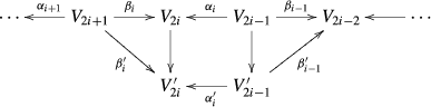
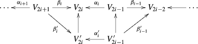
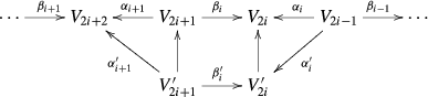
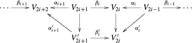
Let \(G_{2m}\) be a directed graph with \(2m\) vertices, \(x_1, x_1, \ldots , x_{2m}\). Its underlying undirected graph is a simple cycle. The directed edges in \(G_{2m}\) are of two types: forward \(a_i: x_{2i-1}\rightarrow x_{2i}\), \(1\le i\le m\), and backward \(b_i: x_{2i+1}\rightarrow x_{2i}\), \(1\le i\le m-1\), \(b_m:x_1\rightarrow x_{2m}\).
We think of this graph as being located on the unit circle centered at the origin o in the plane.
A representation \(\rho \) on \(G_{2m}\) is an assignment of a vector space \(V_x\) to each vertex x and a linear map \(\ell _e: V_{x}\rightarrow V_{y}\) for each oriented edge \(e=\{x,y\}\). Two representations \(\rho \) and \(\rho ^{\prime }\) are isomorphic if for each vertex x there exists an isomorphism from the vector space \(V_x\) of \(\rho \) to the vector space \(V^{\prime }_x\) of \(\rho ^{\prime }\), and these isomorphisms commute with the linear maps \(V_{x}\rightarrow V_{y}\) and \(V^{\prime }_{x}\rightarrow V^{\prime }_{y}\). A non-trivial representation assigns at least one vector space which is not zero-dimensional. A representation is indecomposable if it is not isomorphic to the sum of two non-trivial representations.
Given two representations \(\rho \) and \(\rho ^{\prime }\), their sum \(\rho \oplus \rho ^{\prime }\) is a representation whose vector spaces are the direct sums \(V_x\oplus V^{\prime }_x\) related by linear maps that are the direct sums \(\ell _e\oplus \ell ^{\prime }_e.\) It is not hard to observe that each representation has a decomposition as a sum of indecomposable representations unique up to isomorphisms.
We provide a description of indecomposable representations of the quiver \(G_{2m}.\) For any triple of integers \(\{i,j,k\}\), \(1 \le i,j \le m,\) \(k\ge 0\), one may have any of the four representations, \(\rho ^I([i, j];k), \ \rho ^I((i,j];k), \rho ^I([i,j);k) \), and \(\rho ^I((i,j);k) \) defined below. For any Jordan cell \((\lambda , k)\) one has the representation \(\rho ^J(\lambda , k)\) defined below. The exponents I and J indicate that these representations are associated with a bar code (interval) or a Jordan cell respectively and hence we call them bar code and Jordan cell representations.
-
Bar code representation \(\rho ^I(\{i, j\};k)\): Suppose that the evenly indexed vertices \(\{x_2, x_4, \ldots , x_{2m}\}\) of \(G_{2m}\) which are the targets of the directed arrows correspond to the angles \(0< s_1< s_2 <\cdots <s_{m} \le 2\pi .\) Draw the spiral curve given by (1) for the interval \(\{s_{i}, s_{j}+2k\pi \}\); refer to Fig. 3. For each \(x_i\), let \(\{e_i^1,e_i^2,\ldots \}\) denote the ordered set (possibly empty) of intersection points of the ray \(ox_i\) with the spiral. While considering these intersections, it is important to realize that the point \((x(s_i), y(s_i))\) (resp. \((x(s_j+2k\pi ), y(s_j+2k\pi ))\)) does not belong to the spiral (1) if \(\{i,j\}\) is open at \(i\) (resp. \(j\)). For example, in Fig. 3, the last circle on the ray \(ox_{2j}\) is not on the spiral since \([i,j)\) in \(\rho ^I([i,j);2)\) is open at right. Let \(V_{x_i}\) denote the vector space generated by the base \(\{e_i^1,e_i^2,\ldots \}\). Furthermore, let \(\alpha _i: V_{x_{2i-1}}\rightarrow V_{x_{2i}}\) and \(\beta _i: V_{x_{2i+1}}\rightarrow V_{x_{2i}}\) be the linear maps defined on bases and extended by linearity as follows: assign the vector \(e^h_{2i}\in V_{x_i}\) to \(e^{\ell }_{2i\pm 1}\) if \(e^h_{2i}\) is an adjacent intersection point to the points \(e^{\ell }_{2i\pm 1}\) on the spiral. If \(e^h_{2i}\) does not exist, assign zero to \(e^{\ell }_{2i\pm 1}\). If \(e^{\ell }_{2i\pm 1}\) does not go to zero, \(h\) has to be \(l\), \(l-1\), or \(l+1\). The construction above provides a representation on \(G_{2m}\) which is indecomposable. Once the angles \(s_i\) are associated to the vertices \(x_{2i}\) one can also think of these representations \(\rho ^I(\{i,j\};k)\) as the bar codes \([s_{i}, s_{j}+2k\pi ]\), \((s_{i}, s_{j}+2k\pi ], [s_{i}, s_{j}+2k\pi )\), and \((s_{i}, s_{j}+2k\pi )\).
-
Jordan cell representation \(\rho ^J(\lambda ,k)\): Assign the vector space with the base \(\{e_1,e_2,\ldots ,e_k\}\) to each \(x_i\) and take all linear maps \(\alpha _i\) but one (say \(\alpha _1\)) and \(\beta _i\) the identity. The linear map \(\alpha _1\) is given by the Jordan matrix defined by \((\lambda ,k)\) in (2). Again this representation is indecomposable.

The spiral for \([s_i,s_j+4\pi )\)
It follows from the work of [11, 18] that when \(\kappa \) is algebraically closed,Footnote 5 the bar code and Jordan cell representations are all and only indecomposable representations of the quiver \(G_{2m}.\) The collection of all bar code and Jordan cell representations of a representation \(\rho \) constitutes its invariants.
Now, consider the representation \(\rho \) on the graph \(G_{2m}\) given by the vector spaces \(V_{2i-1}:=V_{x_{2i- 1}}, V_{2i}:=V_{x_{2i}}\) and the linear maps \(\alpha _i\) and \(\beta _i.\) To such a representation \(\rho \), we associate a map \(M_\rho : \bigoplus _{1\le i\le m} V_{2i- 1} \rightarrow \bigoplus _{1\le i\le m}V_{2i}\) which is represented by a block matrix also denoted as \(M_{\rho }\):
For this representation we define its dimension characteristic as the \(2m\)-tuple of positive integers
with \(n_i= \dim V_{x_{2i-1}}\) and \(r_i=\dim V_{x_{2i}}\) and denote by \(\ker \rho := \ker M_\rho \) and \(\mathrm coker\ \rho = \mathrm coker\ M_\rho .\) For the sum of two such representations \(\rho = \rho _1 \oplus \rho _2\) we have:
Proposition 4.1
-
1.
\(\dim (\rho _1\oplus \rho _2)= \dim \rho _1 + \dim \rho _2 \),
-
2.
\(\dim \ker (\rho _1\oplus \rho _2)=\dim \ker \rho _1 + \dim \ker \rho _2\),
-
3.
\(\dim \mathrm coker\ (\rho _1\oplus \rho _2)= \dim \mathrm coker\ \rho _1 + \dim \mathrm coker\ \rho _2\).
The description of a bar code representation permits explicit calculations.
Proposition 4.2
-
1.
If \(i\le j\) then
-
(a)
\(\dim \rho ^I([i,j]; k)\) is given by: \(n_l=k+1\) if \((i+1)\le l\le j\) and k otherwise, \( r_l= k+1\) if \(i\le l\le j\) and k otherwise
-
(b)
\(\dim \rho ^I((i,j]; k)\) is given by: \(n_l=k+1\) if \((i+1)\le l\le j\) and k otherwise, \(r_l= k+1\) if \((i +1)\le l\le j\) and k otherwise,
-
(c)
\(\dim \rho ^I([i,j); k)\) is given by: \(n_l=k+1\) if \((i+1)\le l\le j\) and k otherwise, \( r_l= k+1\) if \(i\le l\le (j-1)\) and k otherwise,
-
(d)
\(\dim \rho ^I((i,j); k)\) is given by: \(n_l=k+1\) if \((i+1)\le l\le j\) and k otherwise, \(r_l= k+1\) if \((i +1)\le l\le ( j-1)\) and k otherwise
-
(a)
-
2.
If \(i> j\) then similar statements hold.
-
(a)
\(\dim \rho ^I([i,j]; k)\) is given by: \(n_l=k\) if \((j+1)\le l\le i\) and \(k+1\) otherwise; \(r_l=k\) if \((j+1)\le l\le (i-1)j\) and \(k+1\) otherwise
-
(b)
\(\dim \rho ^I((i,j]; k)\) is given by: \(n_l=k\) if \((j+1)\le l\le i\) and \(k+1 \) otherwise. \(r_l=k\) if \((j+1)\le l\le i\) and \(k +1\) otherwise,
-
(c)
\(\dim \rho ^I([i,j); k)\) is given by: \(n_l=k\) if \((j+1)\le l\le i\) and \(k+1\) otherwise; \(r_l=k\) if \( j\le l \le (i-1)\) and \(k+1 \) otherwise,
-
(d)
\(\dim \rho ^I((i,j); k)\) is given by: \(n_l=k\) if \((j+1)\le l\le i\) and \(k+1\) otherwise; \(r_l=k\) if \(j\le l\le i\) and \(k+1\) otherwise.
-
(a)
-
3.
\(\dim \rho ^J(\lambda ,k)\) is given by \(n_i=r_i=k\)
Proposition 4.3
-
1.
\(\dim \ker \rho ^I([i,j]; k)=0\), \(\dim \mathrm coker\ \rho ^I([i,j]; k)=1\),
-
2.
\(\dim \ker \rho ^I([i,j); k)=0\), \(\dim \mathrm coker\ \rho ^I([i,j); k)=0\),
-
3.
\(\dim \ker \rho ^I ((i,j]; k)=0\), \(\dim \mathrm coker\ \rho ^I((i,j]; k)=0\),
-
4.
\(\dim \ker \rho ^I((i,j); k)=1\), \(\dim \mathrm coker\ \rho ^I((i,j); k)=0\),
-
5.
\(\dim \ker \rho ^{J}(\lambda ,k) =0\) (resp. 1) if \(\lambda {\ne 1}\) (resp. 1),
-
6.
\(\dim \mathrm coker\ \rho ^{J}(\lambda ,k)=0\) (resp. 1) if \(\lambda {\ne 1}\) (resp. 1).
Observation 4.4
A representation \(\rho \) has no indecomposable components of type \(\rho ^I\) in its decomposition iff all linear maps \(\alpha _i^{\prime }\)s and \(\beta _i^{\prime }\)s are isomorphisms. For such a representation, starting with an index \(i,\) consider the linear isomorphism
The Jordan canonical form [12] of the isomorphism \(T_i\) is independent of \(i\) and is a block diagonal matrix with the diagonal consisting of Jordan cells \((\lambda , k)\)s. Clearly, \(\rho \) is the direct sum of \(\rho ^J(\lambda ,k)\)s, the Jordan cell representations of \(\rho \).
Definition 4.5
(\(r\)-Invariants.) Let f be a circle-valued tame map defined on a topological space X. For f with m critical angles \(0< s_1< s_2,\ldots , s_m\le 2\pi \), consider the quiver \(G_{2m}\) with the vertices \(x_{2i}\) identified with the angles \( s_i\) and the vertices \(x_{2i-1}\) identified with the angles \(t_i\) that satisfy \(0<t_1<s_1<t_2 < s_2, \ldots , t_m<s_m.\)
For any \(r\), consider the representation \(\rho _r\) of \(G_{2m}\) with \(V_{x_i}=H_r(X_{x_i})\) and the linear maps \(\alpha _i\)s and \(\beta _i\)s induced in the \(r\)-homology by maps \(a_i: X_{x_{2i-1}} \rightarrow X_{x_{2i}}\) and \(b_i: X_{x_{2i+1}} \rightarrow X_{x_{2i}}\) described in Sect. 2. The bar code and Jordan cell representations of \(\rho _r\) are independent of the choice of \(t_i\)s and are collectively referred as the r-invariants of \(f.\)
5 Proof of the Main Results
Figure 2 and the bar codes listed below suggest why a semi-closed (one end open and the other closed) bar code does not contribute to the homology of the total space X and why a closed bar code (both ends closed) in \(\mathcal{B}_r\) contributes one unit while an open (both ends open) bar code in \(\mathcal{B}_{r-1}\) contributes one unit to the \(H_r(X)\). Indeed, in our example, a semi-closed bar code in \(\mathcal{B}_1\) adds to the total space a cone over \(\mathbb{S }^1,\) which is a contractible space. It gets glued to the total space along a generator of the cone (a segment connecting the apex to \(\mathbb{S }^1\)), again a contractible space. A closed bar code in \(\mathcal{B}_1\) adds a cylinder of \(\mathbb{S }^1\) whose \(H_1\) has dimension \(1\). It gets glued to the total space along a generator of the cylinder (a segment connecting the same point on the two copies of \(\mathbb{S }^1\)), again a contractible space. An open bar code in \(\mathcal{B}_1\) adds the suspension over \(\mathbb{S }^1\), topologically a \(2\)-sphere which gets glued along a meridian, a contractible space. This contributes a dimension to \(H_2\).
The lack of contribution of a Jordan cell with \(\lambda \ne 1\) as well as the contribution of one unit of a Jordan cell in \(\mathcal{J}_r\) with \(\lambda =1\) to both \(r\) and \(r+1\) dimensional homology of the total space should not be a surprise for the reader familiar with the calculation of the homology of mapping torus.
Below we explain rigorously but schematically the arguments for the proof of Theorems 3.1, 3.2, and Corollary 3.4.
The proof of Theorem 3.1 is a consequence of Propositions 4.1 and 4.2. The proof of Theorem 3.2 proceeds along the following lines.
First observe that, up to homotopy, the space X can be regarded as the iterated mapping torus \(\mathcal T \) described below. Consider the collection of spaces and continuous maps:
with \(R_i:=X_{t_i}\) and \(X_i:= X_{s_i}\) and denote by \(\mathcal T =T(\alpha _1 \cdots \alpha _m; \beta _1\cdots \beta _m)\) the space obtained from the disjoint union
by identifying \(R_i\times \{1\}\) to \(X_i\) by \(\alpha _i\) and \(R_i\times \{0\}\) to \(X_{i-1}\) by \(\beta _{i-1}.\) Denote by \(f^\mathcal{T }:\mathcal T \rightarrow [0,m]\) where \(f^\mathcal{T }: R_i\times [0,1]\rightarrow [i-1,i]\) is the projection on \([0,1]\) followed by the translation of \([0,1]\) to \([i-1,i]\). This map is a homotopical reconstruction of \(f: X \rightarrow \mathbb{S }^1\) provided that, with the choice of angles \(t_i, s_i\) and maps \(a_i\) \(b_i\) described in Sect. 2, \(X_i:= f^{-1}(s_i), R_i:= f^{-1}(t_i)\).
Let \(\mathcal P ^{\prime }\) denote the space obtained from the disjoint union
by identifying \(R_i\times \{1\}\) to \(X_i\) by \(\alpha _i,\) and \(\mathcal P ^{\prime \prime }\) denote the space obtained from the disjoint union
by identifying \(R_i\times \{0\}\) to \(X_{i-1}\) by \(\beta _{i-1}.\)
Let \(\mathcal R = \bigsqcup _{1\le i\le m} R_i\) and \(\mathcal X = \bigsqcup _{1\le i\le m} X_i.\) Then, one has:
-
1.
\(\mathcal T = \mathcal P ^{\prime } \cup \mathcal P ^{\prime \prime }\),
-
2.
\(\mathcal P ^{\prime } \cap \mathcal P ^{\prime \prime }= (\bigsqcup _{1\le i\le m} R_i\times (\varepsilon ,1-\varepsilon ))\sqcup \mathcal X \), and
-
3.
the inclusions \((\bigsqcup _{1\le i\le m} R_i\times \{ 1/2 \})\sqcup \mathcal X \subset \mathcal P ^{\prime }\cap \mathcal P ^{\prime \prime }\) as well as the obvious inclusions \(\mathcal X \subset \mathcal P ^{\prime }\mathrm{and} \mathcal X \subset \mathcal P ^{\prime \prime }\) are homotopy equivalences.
The Mayer–Vietoris long exact sequence leads to the diagram

Here \(\Delta \) denotes the diagonal, \(in_2\) the inclusion on the second component, \(pr_1\) the projection on the first component, \(i^r\) the linear map induced in homology by the inclusion \(\mathcal X \subset \mathcal T \), and \(M_{\rho _r}\) the map given by the matrix
with \(\alpha ^r_i : H_r(R_i)\rightarrow H_r(X_i)\) and \(\beta ^r_i: H_r(R_{i+1})\rightarrow H_r(X_i)\) induced by the maps \(\alpha _i\) and \(\beta _i,\) and N defined by
where \(\alpha ^r\) and \(\beta ^r\) are the matrices
From the diagram above we retain only the long exact sequence
from which we derive the short exact sequence
and then
Theorem 3.2 follows from Propositions 4.1, 4.3 and Eqs. (6) above. A specified decomposition of \(\rho _r\) and \(\rho _{r-1}\) into indecomposable representations and a splitting in the sequence (5) provide specified elements in \(H_r(X_\theta )\) and \(H_r(\mathcal T )\) which can be compared. This leads to the verification of Proposition 3.3.
6 Algorithm
Given a circle-valued tame map \(f:X\rightarrow \mathbb S ^1\), we now present an algorithm to compute the bar codes and the Jordan cells when X is a finite simplicial complex, and f is generic and linear. This makes the map tame. Genericity means that f is injective on vertices. To explain linearity we recall that, for any simplex \(\sigma \in X\), the restriction \(f|_{\sigma }\) admits liftings \(\hat{f}:\sigma \rightarrow \mathbb R \), i.e. \(\hat{f}\) is a continuous map which satisfies \(p\cdot \hat{f}= f|_\sigma .\) The map \(f: X\rightarrow \mathbb S ^1\) is called linear if for any simplex \(\sigma \), at least one of the liftings (and then any other) is linear.
Our algorithm takes the simplicial complex X equipped with the map f as input and, for any \(r\), computes the matrix \(M_{\rho _r}\) of the representation \(\rho _r\) for f. This requires recognizing the critical values \(s_1, s_2, \ldots , s_{m}\in \mathbb S ^1\) of f, and for conveniently chosen regular values \(t_1, t_2, \ldots , t_{m}\in \mathbb S ^1\), determining the vector spaces \(V_{2i-1}=H_r(X_{t_i}), V_{2i}=H_r(X_{s_i})\) with the linear maps \(\alpha _i\) and \(\beta _i\) as matrices. We consider the block matrix \(M_{\rho _r}: \bigoplus _{1\le i\le m} V_{2i-1} \rightarrow \bigoplus _{1\le i\le m}V_{2i}\) described in the previous section.
We compute the bar codes from the block matrix \(M_{\rho _r}\) first, and then the Jordan cells. The algorithm consists of three steps. We describe the first and second steps in sufficient details. The third step is a routine application of Observation 4.1 and is accomplished by standard algorithms in linear algebra (reduction of the matrix to the canonical Jordan form).
-
Step 1. Compute the matrices \(\alpha _i\), \(\beta _i\) that constitute the matrix \(M_{\rho _r}\) of the representation \(\rho _r\).
-
Step 2. Process the matrix of \(M_{\rho _r}\) to derive the bar codes ending up with a representation \(\rho ^{\prime }_r\) whose all \(\alpha _i^{\prime }\)s and \(\beta _i^{\prime }\)s are invertible matrices.
-
Step 3. Compute the Jordan cells of \(\rho _r\) from the representation \(\rho _r^{\prime }.\)
Step 1. In Step 1 we begin with the incidence matrix of the input simplicial complex X equipped with the map \(f:X\rightarrow \mathbb{S }^1.\) Let the angles \(0\le s_1 < s_2\cdots s_m \le 2\pi \) be the critical values of f. Choose a collection of regular angles \(0 <t_1<t_2\cdots t_m <2\pi \) with \(t_{i}< s_{i} <t_{i+1} < s_{i+1}\). Consider a canonical subdivision of X into a cell complex so that \(X_{[t_{i}, t_{i+1}]}\), and \(X_{t_i}\) are subdivided into subcomplexes \(R_i\) and \(X_i\) as follows. For any open simplex \(\sigma \) we associate the open cells:
-
1.
\(\sigma (i):=\sigma \cap X_{t_i}\) with \(\dim (\sigma (i))= \dim \sigma -1\) if the intersection is nonempty
-
2.
\(\sigma \langle i\rangle := \sigma \cap X_{(t_i, t_{i+1})}\) with \(\dim \sigma \langle i \rangle = \dim \sigma \) if the intersection is nonempty.
The cells of \(X_i\) are exactly of the form \(\sigma (i)\) and their incidences are given as \(I(\sigma (i), \tau (i))= I(\sigma , \tau )\) where \(I(\sigma ,\tau )=0, +1, {\mathrm{{or}}}-1\) depending on whether \(\tau \) is a coface of \(\sigma \) and whether their orientations match or not. The cells of \(R_i\) consist of cells of \(X_{i}\), \(X_{i+1}\), and all cells of the form \(\sigma \langle i\rangle \). The incidences are given as \(I(\sigma \langle i \rangle , \tau \langle i \rangle )= I(\sigma , \tau )\), \(I(\sigma (i),\sigma \langle i\rangle )=1\), and \(I(\sigma (i+1), \sigma \langle i\rangle )=-1\). All other incidences are zero. Assume that we are given a total order for the simplices of X that is compatible with f and also the incidence relations. This induces a total order for the cells in \(X_i\) and \(X_{i+1}\) and also the cells in \(R_i^{\prime }=R_i\setminus X_{i}\sqcup X_{i+1}\) for any \(1\le i\le m\) with \(X_{m+1}:=X_1\). Impose a total order on \(R_i\) by juxtaposing the total orders of \(X_{i}\), \(X_{i+1}\), and \(R_i^{\prime }\) in this sequence. Clearly, the incidence matrix for \(R_i\) can be derived from the incidence matrix of X.
The incidence matrix of \(A=X_i\sqcup X_{i+1}\) appears in the upper left corner of the matrix for \(R:=R_i\). We obtain the matrices for the linear maps \(\alpha _i:H_r(X_{t_{i}})\rightarrow H_r(X_{s_i})\) and \(\beta _i: H_r(X_{t_{i+1}})\rightarrow H_r(X_{s_{i}})\) by using the persistence algorithm [5, 22] on \(R\) and \(A\) as follows. First, we run the persistence algorithm on the incidence matrix for \(A\) to compute a base of the homology group \(H_r(A)\). We continue the procedure by adding the columns and rows of the matrix for \(R\) to obtain a base of \(H_r(R)\). It is straightforward to compute a matrix representation of the inclusion induced linear map \(H_r(A)\rightarrow H_r(R)\) with respect to the bases computed by the persistence algorithm.
Step 2. Step 2 takes the matrix representation \(M_{\rho _r}\) constructed out of matrices \(\alpha _i, \beta _i\) computed in step 1, and uses four elementary transformations \(T_1(i),T_2(i),T_3(i)\), and \(T_4(i)\) defined below to transform \(M_{\rho _r}\) to \(M_{\rho ^{\prime }_{r}}= T_{\cdots } (\cdots ) M_{\rho _r},\) whose total number of rows and columns is strictly smaller than that of \(M_{\rho _r}\). For convenience, let us write \(\rho =\rho _r\) and \(\rho ^{\prime }=\rho _r^{\prime }\). Each elementary transformation \(T\) modifies the representation \(\rho \) to the representation \(\rho ^{\prime }\) while keeping indecomposable Jordan cell representations unaffected but possibly changing the bar code representations. Some of these bar code representations remain the same, some are eliminated, and some are shortened by one unit as described below. For each elementary transformation we record the changes to reconstruct the original bar codes. The elementary transformations are applied as long as the linear maps \(\alpha _i\) or \(\beta _i\) satisfy some injectivity and surjectivity property. When no such transformation is applicable, the algorithm terminates with all \(\alpha _i\) and \(\beta _i\) being necessarily invertible matrices. At this point the bar codes can be reconstructed reading backwards the eliminations/modifications performed. The Jordan cells then can be obtained as detailed in Step 3.
The elementary transformations modify the bar codes as follows:
-
\(T_1(i)\) shortens the bar codes\((i-1, k\}\) to \((i,k\}\) if \(i\ge 2\) and shortens the bar codes \((m, k\}, m<k\), to \((1, k-m\}\) if \(i=1\).
-
\(T_2(i)\) shortens the bar codes \(\{l, i+km]\) to \(\{l, i-1+km]\) for \(k\ge 0.\)
-
\(T_3(i)\) shortens the bar codes \([i, k\}\) to \([i+1,k\}\) for \(i< m\) and to \([1, k-m\}\) if \(i=m\).
-
\(T_4(i)\) shortens the bar codes \(\{l, (i+1)+km )\) to \(\{l, i+km)\) for \(k\ge 0.\)
It is understood that if an elementary transformation applied to a bar code provides an interval which is not a bar code, then the bar code is eliminated. Consequently \(T_1(i)\) eliminates the bar codes \((i-1, i), (i-1, i]\),Footnote 6 \(T_2(i)\) eliminates the bar codes \([i,i], (i-1,i],\) \(T_3(i)\) eliminates the bar codes \([i,i+1), [i, i] \), and \(T_4(i)\) eliminates the bar codes \((i, i+1), [i, i+1).\)
To decide how many bar codes are eliminated one uses Proposition 6.1 below. Let \(\#\{i,j\}_\rho \) denote the number of bar codes of type \(\{i, j\}.\)
Proposition 6.1
-
1.
\(\# (i,i+1)_\rho = \dim (\ker \beta _i\cap \ker \alpha _{i+1})\)
-
2.
\(\# [i,i]_\rho = \dim (V_{2i}/((\beta _i (V_{2i+1}) + \alpha _i (V_{2i-1}))\)
-
3.
\(\# (i,i+1]_\rho = \dim (\beta _i(V_{2i+1}) +\alpha _i(\ker \beta _{i-1})) - \dim (\beta _i(V_{2i+1}))\)
-
4.
\(\# [i, i+1)_\rho = \dim (\alpha _i(V_{2i-1}) +\beta _i(\ker \alpha _{i+1}))-\dim (\alpha _i(V_{2i-1}))\)
The following diagrams define the elementary transformations and indicate the relation between the representation \(\rho = \{V_i, \alpha _i, \beta _i\}\) and the representation \(\rho ^{\prime } = \{V^{\prime }_i, \alpha ^{\prime }_i, \beta ^{\prime }_i\}\) obtained after applying an elementary transformation.
-
Transformation \(T_1(i)\): \(V^{\prime }_{2i-1}= V_{2i-1}/ \ker \beta _{i-1}, \quad V^{\prime }_{2i}= V_{2i}/ \alpha _{i}(\ker \beta _{i-1} ),\quad V^{\prime }_k= V_k, k= 2i, 2i-1\)
-
Transformation \(T_2(i)\): \(V^{\prime }_{2i}= \beta _i(V_{2i+1}), \quad V^{\prime }_{2i-1}= \alpha ^{-1}_{i}(\beta _i(V_{2i+1})), \quad V^{\prime }_k= V_k, k\ne 2i-1, 2i\)
-
Transformation \(T_3(i)\): \(V^{\prime }_{2i}= \alpha _{i}(V_{2i-1}), \quad V^{\prime }_{2i+1}= \beta _i^{-1}(\alpha _i(V_{2i-1})), \quad V^{\prime }_k= V_k, k\ne 2i, 2i+1\)
-
Transformation \(T_4(i)\): \(V^{\prime }_{2i+1}= V_{2i+1}/ \ker \alpha _{i+1}, \quad V^{\prime }_{2i}= V_{2i}/ \beta _i(\ker \alpha _{i+1} ), \quad V^{\prime }_k= V_k, k\ne 2i, 2i+1.\)


The verification of the properties stated above and the proof of Proposition 6.1 are straightforward for indecomposable representations described in Sect. 4 and therefore for arbitrary representations.
As one can see from the diagrams above, when \(\beta _{i-1}\) is injective, the representations \(\rho \) and \(\rho ^{\prime }\) are the same and we say that \(T_1(i)\) is not applicable. Similarly, when \(\beta _{i}\) is surjective, \(T_2(i)\) is not applicable, when \(\alpha _{i}\) is surjective, \(T_3(i)\) is not applicable, and when \(\alpha _{i+1}\) is injective, \(T_4(i)\) is not applicable. When all \(\alpha _i, \beta _i\) are invertible, no elementary transformation is applicable and at this stage the algorithm (Step 2) terminates.
To explain how the algorithm works, it is convenient to consider the following block matrices \(B_{2i-1}\) and \(B_{2i}\), \(i=1,\ldots ,m\), which become the sub-matrices of \(M_{\rho _r}\) in (3) when the entries \(\beta _i\) are replaced with \(-\beta _i\). Let
for \(i= 1,2,\ldots , (m-1)\) and
We modify \(M_\rho \) by modifying successively each block \(B_k.\) When \(m>1\) the algorithm iterates over the blocks in multiple passes. In a single pass, it processes the blocks \(B_1, B_2,\ldots ,B_{2m}\) in this order.
When
is processed then:
-
1.
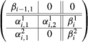
If \(\beta _{i-1}\) is not injective, we apply \(T_1(i).\) This boils down to changing the bases of \(V_{2i-1}\) and \(V_{2i}\) so that the matrix \(B_{2(i-1)}\) becomes
with (\(\beta _{i-1,1} \, 0\)) in column echelon form and
$$\begin{aligned} \left( \begin{array}{c}\alpha ^1_{i,2}\\ 0\end{array}\right) \end{aligned}$$in row echelon form. In this block matrix the first and third columns correspond to \(V^{\prime }_{2i-1}\) and \(V_{2i+1}\) respectively, and the first and third rows to \(V_{2(i-1)}\) and \(V^{\prime }_{2i}\) respectively. The second column and row become “irrelevant” as a result of which the modified block matrix \(B_{2(i-1)}\) becomes
$$\begin{aligned} \left( \begin{array}{cc}\beta ^{\prime }_{i-1}&{}\quad 0\\ \alpha ^{\prime }_i&{}\beta ^{\prime }_i\end{array}\right) = \left( \begin{array}{cc}\beta _{i-1,1}&{}\quad 0\\ \alpha ^2_{i,1}&{} \quad \beta ^2_{i} \end{array}\right) . \end{aligned}$$ -
2.
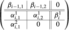
If \(\beta _{i}\) is not surjective, we apply \(T_2(i).\) This boils down to changing the bases of \(V_{2i-1}\) and \(V_{2i}\) so that the matrix \(B_{2(i-1)}\) becomes
with
$$\begin{aligned} \left( \begin{array}{c}\beta ^1_{i}\\ 0 \end{array}\right) \end{aligned}$$in row echelon form and (\(\alpha ^2_{i,1}\, 0\)) in column echelon form. In this block matrix the second and third columns correspond to \(V^{\prime }_{2i-1}\) and \(V_{2i+1}\) respectively, and the first and second rows to \(V_{2(i-1)}\) and \(V^{\prime }_{2i}\) respectively. We make the first column and third row “irrelevant” as a result of which the modified block matrix \(B_{2(i-1)}\) becomes
$$\begin{aligned} \left( \begin{array}{cc}\beta ^{\prime }_{i-1}&{}\quad 0\\ \alpha ^{\prime }_i&{}\quad \beta ^{\prime }_i\end{array}\right) = \left( \begin{array}{cc}\beta _{i-1,2}&{}\quad 0\\ \alpha ^1_{i,2}&{} \quad \beta ^1_{i}\end{array}\right) . \end{aligned}$$When \(B_{2i-1}\) is processed then:
-
3.
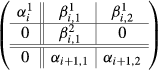
If \(\alpha _i\) is not surjective, we apply \(T_3(i).\) This boils down to changing the bases of \(V_{2i+1}\) and \(V_{2i}\) so that the matrix \(B_{2i-1}\) becomes
with
$$\begin{aligned} \left( \begin{array}{c}\alpha ^1_{i}\\ 0\end{array}\right) \end{aligned}$$in row echelon form and \(\beta ^2_{i,1}\, 0\) in column echelon form. In this block matrix the first and third columns correspond to \(V_{2i-1}\) and \(V^{\prime }_{2i+1}\) respectively, and the first and third rows to \(V^{\prime }_{2i}\) and \(V_{2i+2}\) respectively. We make the second column and second row “irrelevant” as a result of which the modified block matrix \(B_{2i-1}\) becomes
$$\begin{aligned} \left( \begin{array}{cc}\alpha ^{\prime }_{i}&{}\quad \beta ^{\prime }_i\\ 0&{}\quad \alpha ^{\prime }_{i+1}\end{array}\right) = \left( \begin{array}{cc}\alpha ^1_{i}&{}\quad \beta ^1_{i,2}\\ 0 &{}\quad \alpha _{i+1,2}\end{array}\right) . \end{aligned}$$ -
4.
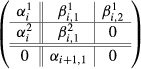
If \(\alpha _{i+1}\) is not injective, we apply \(T_4(i).\) This boils down to changing the bases of \(V_{2i+1}\) and \(V_{2i}\) so that the matrix \(B_{2i-1}\) becomes
with (\(\alpha _{i+1,1}\,0 \)) in column echelon form and
$$\begin{aligned} \left( \begin{array}{c}\beta ^1_{i,2}\\ 0\end{array}\right) \end{aligned}$$in row echelon form. In this block matrix first and second columns correspond to \(V_{2i-1}\) and \(\ V^{\prime }_{2i+1}\) respectively, and second and third rows to \(V_{2i}^{\prime }\) and \(V_{2(i+1)}\) respectively. We make the third column and first row “irrelevant” as a result of which the modified block matrix \(B_{2i-1}\) becomes
$$\begin{aligned} \left( \begin{array}{cc}\alpha ^{\prime }_{i}&{}\quad \beta ^{\prime }_i\\ 0&{}\quad \alpha ^{\prime }_{i+1}\end{array}\right) = \left( \begin{array}{cc}\alpha ^2_{i}&{}\quad \beta ^2_{i,1}\\ 0&{}\quad \alpha _{i+1,1}\end{array}\right) . \end{aligned}$$


Explicit formulae for \(\alpha ^{\prime }\)s and \(\beta ^{\prime }\)s are given at the end of this section. At each pass the algorithm may eliminate or change bar codes, and if this happens, the matrix has less columns or rows. If this does not happen, the algorithm terminates, and indicates that there is no more bar code left. At termination, all \(\alpha _i\) and \(\beta _i\) become isomorphisms. The bar codes can be recovered by keeping track of all eliminations of the bar codes after each elementary transformation. A bar code which is not eliminated in a pass gets shrunk by exactly two units, during that pass, that is, a bar code \(\{i,j\}\) shrinks to \(\{i+1, j-1\}\) by exactly two distinct elementary transformations. by elementary transformations. For example if \(m=5 \) the bar code \((1,5]\) during the pass became \((2,4]\) as result of applying \(T_1(1)\) when inspecting \(B_1\) and \(T_2(5)\) when inspecting \(B_9.\)
When a bar code \([i,i]\) is eliminated, say, in the kth pass, we know that it corresponds to a bar code \([i-k+1, i+k-1]\) in the original representation. Similarly, other bar codes of type \(\{i,i+1\}\) eliminated at the kth pass correspond to the bar code \(\{i-k+1,i+k\}\). In both cases, the multiplicity of the bar codes can be determined from the multiplicity of the eliminated bar codes thanks to Proposition 6.1.
When \(m=1\), the operations on above minors are not well defined. In this case we extend the quiver \(G_2\) to \(G_4\) (\(m=2\)) by adding fake levels \(t_2, s_2\) where \(H_r(X_{t_2})=H_r(X_{s_2})=H_r(X_{s_1})\) and \(\alpha _2,\beta _2\) are identities.Footnote 7
A high level pseudocode for the Step 2 can be written as follows:

Example.
To illustrate how step 2 works, we consider a representation given by
The reader can notice that this is the representation \(\rho _1\) for a simplified version of the example provided in Fig. 2 with the cylinder between the critical values \(\theta _2\) and \(\theta _3\) removed.
-
Inspect \(B_1\) and \(B_2.\) No changes are necessary.
-
Inspect \(B_3\). Since \(\alpha _3\) is not injective, one modifies the block by applying \(T_4(2)\) which makes both \(\alpha _3\) and \(\beta _2\) equal to
$$\begin{aligned} \left( \begin{array}{cc}1 &{}\quad 0\\ 0 &{}\quad 1\end{array}\right) . \end{aligned}$$ -
Inspect the blocks \(B_4, B_5, B_6, B_7.\) No changes are necessary.
-
Inspect \(B_8\). Since \(\beta _4\) is not injective, one modifies the block by applying \(T_1(1)\) which leads to
$$\begin{aligned} \alpha _1=\left( \begin{array}{cc}-4 &{}\quad 3\\ -3 &{}\quad 0 \end{array}\right) \quad {\mathrm{{and}}}\quad \beta _1=\left( \begin{array}{cc}-1 &{}\quad 1\\ -1 &{}\quad 0\end{array}\right) . \end{aligned}$$
Indeed the block \(B_8\) is given by

Since \(\beta _4\) is already in column echelon form one only has to change the base of \(V_2\) to bring the last column of \(\alpha _1\) in row echelon form which ends up with

Therefore
The algorithm stops as all \(\alpha _i^{\prime }\)s and \(\beta _i^{\prime }\)s are at this time invertible. The last transformation \(T_1(1)\) has eliminated only the bar code \((4,5]\), and the previous, which was the first transformation, \(T_4(2),\) has eliminated only the bar code \((2, 3).\) This can be concluded from Proposition 6.1. In view of the properties of these two transformations, one concludes that these were the only two bar codes.
Step 3. At termination, all \(\alpha _i\) and \(\beta _i\) become isomorphisms because otherwise one of the transformations would be applicable. The Jordan cells can be recovered from the Jordan decomposition of the matrix
Standard linear algebra routines permit the calculation of the Jordan cells for familiar algebraic closed fields. Note that if \(\kappa \) is not algebraically closed, Step 1 and Step 2 can still be performed and the matrix \(T\) can be obtained. In this case it may not be possible to decompose the matrix \(T\) in Jordan cells unless we consider the algebraic closure of \(\kappa \). It is however possible to decompose the matrix \(T\) up to conjugacy as a sum of indecomposable invertible matrices while remaining in the class of matrices with coefficients in the field \(\kappa \). This is the case for the field \(\kappa = \mathbb Z _2\).
In the example above
provides the Jordan cell \((\lambda =3, k=2).\)
6.1 Implementation of \(T_1(i), T_2(i), T_3(i)\) and \(T_4(i).\)
-
1.
\(T_1 (i)\) acts on the block matrix
$$\begin{aligned} B_{2(i-1)}=\left( \begin{array}{cc}\beta _{i-1}&{}\quad 0\\ \alpha _i&{}\quad \beta _i \end{array}\right) . \end{aligned}$$First we modify \(B_{2(i-1)}\) to the block matrix
$$\begin{aligned} \left( \begin{array}{ccc}\beta _{i-1,1}&{}\quad 0&{}\quad 0\\ \alpha _{i,2}&{}\quad \alpha _{i,2}&{} \quad \beta _i \end{array}\right) \end{aligned}$$where \(\begin{array}{cc}\beta _{i-1,1}&\quad 0 \end{array}= \beta _{i-1}\cdot R(\beta _{i-1}) \quad {\mathrm{{and}}}\,\,\begin{array}{cc} \alpha _{i,1}&\quad \alpha _{i,2} \end{array}= \alpha _i\cdot R(\beta _{i-1}).\) Recall the definition of \(R(\cdot )\) and \(L(\cdot )\) given under notations in the introduction. Then, one passes to the block matrix
$$\begin{aligned} \left( \begin{array}{ccc} \beta _{i-1,1}&{}\quad 0&{}\quad 0\\ \alpha ^1_{i,2}&{}\quad \alpha ^1_{i,2}&{}\quad \beta ^1_i\\ \alpha ^2_{i,2}&{}\quad 0&{}\quad \beta ^2_i\end{array}\right) \end{aligned}$$with
$$\begin{aligned} \left( \begin{array}{c}\alpha ^1_{i,2}\\ 0 \end{array}\right) =L(\alpha _{i,2})\cdot \alpha _{i,2}, \left( \begin{array}{c}\alpha ^1_{i,1}\\ \alpha ^2_{i,2} \end{array}\right) =L(\alpha _{i,2}) \cdot \alpha _{i,1} \quad {\mathrm{{and}}}\quad \left( \begin{array}{c}\beta ^1_{i}\\ \beta ^2_i \end{array}\right) =L(\alpha _{i,2})\beta _{i}. \end{aligned}$$The modified block matrix is
$$\begin{aligned} \left( \begin{array}{cc}\beta _{i-1,1}&{}\quad 0\\ \alpha ^2_{i,1}&{}\quad \beta ^2_i \end{array}\right) . \end{aligned}$$ -
2.
\(T_2 (i)\) acts on the block matrix
$$\begin{aligned} B_{2(i-1)}= \left( \begin{array}{cc}\beta _{i-1}&{}\quad 0\\ \alpha _i&{}\quad \beta _i \end{array}\right) . \end{aligned}$$First we modify \(B_{2(i-1)}\) to the block matrix
$$\begin{aligned} \left( \begin{array}{cc} \beta _{i-1}&{}\quad 0\\ \alpha ^1_{i}&{}\quad \beta ^1_i\\ \alpha ^2_i&{}\quad 0 \end{array}\right) \end{aligned}$$where
$$\begin{aligned} \left( \begin{array}{c}\beta ^1_{i}\\ 0\end{array}\right) =L(\beta _i)\cdot \beta _i \quad {\mathrm{{and}}} \,\, \left( \begin{array}{c}\alpha ^1_{i}\\ \alpha ^2_i\end{array}\right) =L(\beta _i)\cdot \alpha _i. \end{aligned}$$Then, one passes to the block matrix
$$\begin{aligned} \left( \begin{array}{ccc}\beta _{i-1,1}&{}\quad \beta _{i-1,2}&{}\quad 0\\ \alpha ^1_{i,1}&{}\quad \alpha ^1_{i,2}&{}\quad \beta ^1_i\\ \alpha ^2_{i,1}&{}\quad 0&{}\quad 0\end{array}\right) \end{aligned}$$with
$$\begin{aligned} \left( \begin{array}{c}\alpha ^2_{i,1}\\ 0 \end{array}\right) \!=\! \alpha ^2_{i,1}\cdot R(\alpha ^2_{i,1}), \left( \begin{array}{c}\alpha ^1_{i,1}\\ \alpha ^1_{i,2} \end{array}\right) \!=\! \alpha _{i,1}R(\alpha ^2_{i,1}), \quad {\mathrm{{and}}} \,\, \left( \begin{array}{c} \beta _{i-1,1}\\ \beta _{i-1,2} \end{array}\right) = \beta _{i-1}R(\alpha _{i,1}). \end{aligned}$$The modified block matrix is
$$\begin{aligned} \left( \begin{array}{cc}\beta _{i-1,2}&{}\quad 0\\ \alpha ^1_{i,2} &{}\quad \beta ^1_i \end{array}\right) . \end{aligned}$$ -
3.
\(T_3 (i)\) acts on the block matrix
$$\begin{aligned} B_{2i-1}= \left( \begin{array}{cc} \alpha _{i}&{}\quad \beta _i\\ 0 &{}\quad \alpha _{i+1} \end{array}\right) . \end{aligned}$$First we modify \(B_{2i-1}\) to the block matrix
$$\begin{aligned} \left( \begin{array}{cc} \alpha ^1_i&{}\quad \beta ^1_i\\ 0 &{}\quad \beta ^2_i\\ 0&{}\quad \alpha _{i+1} \end{array}\right) \end{aligned}$$where
$$\begin{aligned} \left( \begin{array}{c}\alpha ^1_{i}\\ 0\end{array}\right) =\alpha _i\cdot R(\alpha _i) \,\, {\mathrm{{and}}} \left( \begin{array}{c}\beta ^1_{i}\\ \beta ^2_i\end{array}\right) =\beta _i\cdot R(\alpha _i). \end{aligned}$$Then, one passes to the block matrix
$$\begin{aligned} \left( \begin{array}{ccc} \alpha ^1_i&{}\quad \beta ^1_{i,1}&{}\quad \beta ^1_{i,2}\\ 0 &{}\quad \beta ^2_{i,1}&{}\quad 0\\ 0&{}\quad \alpha _{i+1,1}&{}\quad \alpha _{i+1,2}\end{array}\right) \end{aligned}$$with
$$\begin{aligned} \left( \begin{array}{cc}\beta ^2_{i,1}&\quad 0\end{array}\right) = \beta ^2_{i}\cdot R( \beta ^2_{i}), \left( \begin{array}{cc}\beta ^1_{i,1}&\quad \beta ^1_{i,2} \end{array}\right) = \beta ^1_i\cdot R( \beta ^2_{i}) \end{aligned}$$and \(\begin{pmatrix}\alpha _{i+1,1}&\alpha _{i+1,2} \end{pmatrix} = \alpha _{i+1}\cdot R( \beta ^2_{i}).\) The modified block matrix is
$$\begin{aligned} \left( \begin{array}{cc}\alpha ^1_{i}&{}\quad \beta ^1_{i,2}\\ 0 &{}\quad \alpha _{i+1,2}\end{array}\right) . \end{aligned}$$ -
4.
\(T_4 (i)\) acts on the block matrix
$$\begin{aligned} B_{2i-1}=\left( \begin{array}{cc} \alpha _{i}&{}\quad \beta _i\\ 0 &{}\quad \alpha _{i_1} \end{array}\right) . \end{aligned}$$First one modifies \(B_{2i-1}\) to the block matrix
$$\begin{aligned} \left( \begin{array}{ccc} \alpha _i&{}\quad \beta _{i,1}&{}\quad \beta _{i,2} \\ 0&{}\quad \alpha _{i+1,1}&{}\quad 0 \end{array}\right) \end{aligned}$$where
$$\begin{aligned} \left( \begin{array}{cc}\alpha _{i+1,1}&\quad 0\end{array}\right) =\alpha _{i+1}\cdot R(\alpha _{i+1}) \quad {\mathrm{{and}}}\,\, \left( \begin{array}{cc}\beta _{i,1}&\quad \beta _{i,2} \end{array}\right) =\beta _i\cdot R(\alpha _{i+1}). \end{aligned}$$Then, one passes to the block matrix
$$\begin{aligned} \left( \begin{array}{ccc} \alpha ^1_i&{}\quad \beta ^1_{i,1}&{}\quad \beta ^1_{i,2} \\ \alpha ^2_i&{} \beta ^2_{i,1}&{}\quad 0\\ 0 &{}\quad \alpha ^2_{i+1,1}&{}\quad 0\end{array}\right) \end{aligned}$$with
$$\begin{aligned} \left( \begin{array}{c}\beta ^1_{i,2}\\ 0 \end{array}\right) = L(\beta _{i,2})\cdot \beta _{i,2}, \left( \begin{array}{c}\beta ^1_{i,1}\\ \beta ^2_{i,1} \end{array}\right) =L(\beta _{i,2})\cdot \beta _{i,1} \quad {\mathrm{{and }}}\,\, \left( \begin{array}{c}\alpha ^1_{i}\\ \alpha ^2_{i} \end{array}\right) = L(\beta _{i,2})\cdot \alpha _{i}. \end{aligned}$$The modified block matrix is
$$\begin{aligned} \left( \begin{array}{cc}\alpha ^2_i&{}\quad \beta ^2_{i,1}\\ 0&{}\quad \alpha _{i+1,1}\end{array}\right) . \end{aligned}$$
6.2 Time Complexity
Let the input complex X have n simplices in total on which the circle-valued map f is defined which has m critical values.
Then, step 1 takes \(O(nd)\) time to detect all the critical values where \(d\le n\) is the maximum degree of any vertex. The critical values can be computed by looking at the simplices adjacent to each of the vertices. To compute the matrices \(\alpha _i\) and \(\beta _i\), we set up the matrices of size \(O(n)\times O(n)\) and run persistence on them. Using the algorithm of [17], this can be achieved in \(O(M(n))\) time where \(M(n)\) is the time complexity of multiplying two \(n\times n\) matrices.Footnote 8 Since we perform this operations for each of the critical levels and the spaces between them, we have \(O(m M(n))\) total time complexity for step 1.
In step 2, we process the matrix \(M_{\rho _r}\) iteratively until all bar code representations are removed. In each pass except the last one, we are guaranteed to shrink a bar code by at least one unit. Therefore, the total number of passes is bounded from above by the total length of all bar codes. Theorem 3.1 implies that a bar code cannot come back to the same level more than \(\max _{s_i} \dim H_r(X_{s_i})\) times which can be at most \(O(n)\). Therefore, any bar code has a length of at most \(O(nm)\) giving a total length of \(O(n^2m)\) over all bar codes. Hence, the repeat loop in the algorithm BarCode cannot have more that \(O(n^2m)\) iterations. In each iteration, we reduce the block matrices each of which can be done with \(O(M(n))\) matrix multiplication time [16]. Since there are at most \(O(m)\) block matrices to be considered, we have \(O(m M(n))\) time per iteration giving a total of \(O(n^2m^2 M(n))\) time for step 2.
Step 3 is performed on the resulting matrix from step 2 which has \(O(mn)\times O(mn)\) size. This can again be performed by matrix multiplication which takes \(O(M(mn))\) time.
Therefore, the entire algorithm has time complexity of \(O(m^2n^2 M(n)+ M(mn))\).
7 Conclusions
We have analyzed circle-valued maps from the perspective of topological persistence. We show that the notion of persistence for such maps incorporate an invariant that is not encountered in persistence studied erstwhile. Our results also shed lights on computing homology vector spaces and other topological invariants from bar codes and Jordan cells (Theorems 3.1 and 3.2). We have given an algorithm to compute the bar codes and the Jordan cells; the algorithms can also be adapted to compute zig-zag persistence. In a subsequent work, Burghelea and Haller have derived more subtle topological invariants like Novikov homology, monodromy [2], Reidemeister torsion, and others from bar codes and Jordan cells confirming their mathematical relevance. We have not treated in this paper the stability of the invariants; see [2] for partial answer.
The standard persistence is related to Morse theory. In a similar vein, the persistence for circle-valued map is related to Morse Novikov theory [19]. The work of Burghelea and Haller applies Morse Novikov theory to instantons and closed trajectories for vector field with Lyapunov closed one form [1]. The results in this paper will very likely provide additional insight on the dynamics of these vector fields and have implications in computational topology in particular and algebraic topology in general.
Notes
It was brought to our attention by David Cohen-Steiner that the extended persistence proposed in [7] allows similar connections between homology of source spaces and persistence.
Since the map f is proper and \(\mathbb S ^1\) compact, so is X.
The white circles indicate open ends and the dark circles indicate closed ends.
Each circle is oriented counterclockwise and represents a 1-dimensional homology class; “k times (\(-k\) times) around the circle” means “going around k times counter clockwise (clockwise respectively)”.
Fig. 2 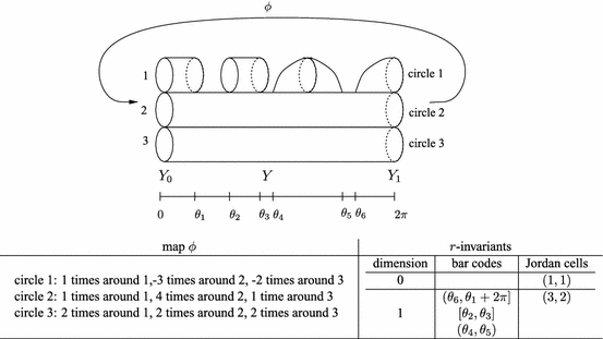
Example of r-invariants for a circle-valued map
When \(\kappa \) is not algebraically closed Jordan cells have to be replaced by conjugate classes of indecomposable (not conjugated to a direct sum of matrices) matrices with entries in \(\kappa \).
If \(i=1\) eliminates the bar codes \((m,m+1)\) and \((m,m+1]\).
Other easier methods can also be used in this case.
We have \(M(n)=O(n^{\omega })\) where \(\omega < 2.376\) [8].

References
Burghelea, D., Haller, S.: Laplace transform and spectral geometry. J. Topol. Dyn. 1, 115–151 (2008)
Burghelea, D., Haller, S.: Graph representations and topology of real and angle valued maps. http://arXiv/abs/1202.1208 (2012)
Burghelea, D., Dey, T.K., Dong, D.: Defining and computing topological persistence for 1-cocycles. http://arXiv/abs/1012.3763 (2010)
Carlsson, G., de Silva, V., Morozov, D.: Zigzag persistent homology and real-valued functions. In: Proceedings of the 25th Annual Symposium on Computational Geometry, pp. 247–256. ACM, New York (2009)
Cohen-Steiner, D., Edelsbrunner, H., Morozov, D.: Vines and vineyards by updating persistence in linear time. In: Proceedings of the 22th Annual Symposium on Computational Geometry, pp. 119–134. ACM, New York (2006)
Cohen-Steiner, D., Edelsbrunner, H., Harer, J.L.: Stability of persistence diagrams. Discrete Comput. Geom. 37, 103–120 (2007)
Cohen-Steiner, D., Edelsbrunner, H., Harer, J.: Extending persistence using Poincaré and Lefschetz duality. Found. Comput. Math. 9(1), 79–103 (2009)
Coppersmith, D., Winograd, S.: Matrix multiplication via arithmetic progressions. J. Symb. Comput. 9(3), 251–280 (1990)
de Silva, V., Vejdemo-Johansson, M.: Persistent cohomology and circular coordinates. In: Proceedings of the 25th Annual Symposium on Computational Geometry, pp. 227–236. ACM, New York (2009)
Dey, T.K., Wenger, R.: Stability of critical points with interval persistence. Discrete Comput. Geom. 38, 479–512 (2007)
Donovan, P., Freislich, M.R.: Representation theory of finite graphs and associated algebras. Carleton Mathematical Lecture Notes No. 5, Carleton University, Ottawa (1973)
Dunford, N., Schwartz, J.T.: Linear Operators, Part I: General Theory. Wiley-Interscience, New York (1958)
Edelsbrunner, H., Harer, J.L.: Computational Topology: An Introduction. American Mathematical Society, Providence, RI (2009)
Edelsbrunner, H., Letscher, D., Zomorodian, A.: Topological persistence and simplification. Discrete Comput. Geom. 28, 511–533 (2002)
Gabriel, P.: Unzerlegbare Darstellungen I. Manuscr. Math. 6, 71–103 (1972)
Jeannerod, C.: LSP matrix decomposition revisited. http://www.ens-lyon.fr/LIP/Pub/Rapports/RR/RR2006/RR2006-28.pdf (2006)
Milosavljević, N., Morozov, D., Škraba P.: Zigzag persistent homology in matrix multiplication time. In: Proceedings of the 27th Annual Symposium on Computational Geometry, pp. 216–225. ACM, New York (2011)
Nazarova, L.A.: Representations of quivers of infinite type (Russian). IZV. Akad. Nauk SSSR Ser. Mat. 37, 752–791 (1973)
Novikov, S.P.: Quasiperiodic structures in topology. In: Goldberg L.R., Phillips A.V. (eds.), Topological Methods in Modern Mathematics. Proceedings of the Symposium in Honor of John Milnor’s Sixtieth Birthday, Stony Brook, NY (1991). Publish or Perish, Houston, TX, pp. 223–233 (1993)
Xiaoye, J., Lek-Heng, L., Yuan, Y., Yinyu, Y.: Statistical ranking and combinatorial Hodge theory. http://arxiv/abs/0811.1067 (2008)
Yuan, Y.: Combinatorial laplacians and rank aggregation. In: The 6th International Congress of Industrial and Applied Mathematics (ICIAM), Mini Symposium: Novel Matrix Methods for Internet Data Mining, Zurich, 16–20 July, 2007
Zomorodian, A., Carlsson, G.: Computing persistent homology. Discrete Comput. Geom. 33, 249–274 (2005)
Acknowledgments
We acknowledge the support of the NSF Grant CCF-0915996 which made this research possible. We also thank all the referees whose comments were helpful in improving the presentation of the paper.
Author information
Authors and Affiliations
Corresponding author
Appendix
Appendix
In this appendix we explain the calculation of the \(r\)-invariants for the example depicted in Fig. 2. The representation \(\rho _0\) has vector spaces that are all one dimensional and maps \(\alpha _i= \beta _i\) that are all identity. Hence, there is no bar code, but one Jordan cell \(\lambda =1, k=1.\)
It is not hard to recognize from Fig. 2 that the maps for the representation \(\rho _1\) are given by:
We proceed with the step 2 of the algorithm.
-
inspect \(B_1\)—no change for \(\rho = \rho _1\); inspect \(B_2\)—no change.
-
inspect \(B_3\)—since \(\alpha _2\) is not surjective apply \(T_3(2).\) This changes \(\alpha _2, \beta _2, \alpha _3\) into
$$\begin{aligned} \alpha ^{\prime }_2= \left( \begin{array}{cc}1&{}\quad 0\\ 0&{}\quad 1\end{array}\right) , \beta ^{\prime }_2= \left( \begin{array}{cc}1&{}\quad 0\\ 0&{}\quad 1\end{array}\right) , \alpha ^{\prime }_3= \left( \begin{array}{cc}1&{}\quad 0\\ 0&{}\quad 1\\ 0&{}\quad 0\end{array}\right) . \end{aligned}$$Update and continue.
-
inspect \(B_4\)—no changes.
-
inspect \(B_5\)—since \(\alpha _3\) is not surjective, apply \(T_3(3).\) This changes \(\alpha _3\) and \(\beta _3\) into
$$\begin{aligned} \alpha ^{\prime }_3= \left( \begin{array}{cc}1&{}\quad 0\\ 0&{}\quad 1\end{array}\right) \quad {\mathrm{{and}}}\,\, \beta ^{\prime }_3= \left( \begin{array}{cc}1&{}\quad 0\\ 0&{}\quad 1 \end{array}\right) . \end{aligned}$$Update and continue.
-
inspect \(B_6\)—no changes.
-
inspect \(B_7\)—since \(\alpha _5\) is not injective, apply \(T_4(4).\) This changes \(\beta _4\) and \(\alpha _5\) into
$$\begin{aligned} \alpha ^{\prime }_5= \left( \begin{array}{cc}1&{}\quad 0\\ 0&{}\quad 1\end{array}\right) \,\, {\mathrm{{and}}}\,\, \beta ^{\prime }_4= \left( \begin{array}{cc}1&{}\quad 0\\ 0&{}\quad 1\end{array}\right) . \end{aligned}$$Update and continue.
-
inspect \(B_8\)—no change; inspect \(B_9\)—no change; inspect \(B_{10}\)—no change; inspect \(B_{11}\)—no change.
-
inspect \(B_{12}\)—since \(\beta _6\) is not injective, apply \(T_1(1).\) This changes \(\beta _6\), \(\alpha _1,\) \(\beta _1\) to
$$\begin{aligned} \beta ^{\prime }_6= \left( \begin{array}{cc}1&{}\quad 0\\ 0&{}\quad 1\end{array}\right) , \alpha ^{\prime }_1= \left( \begin{array}{cc}-4&{}\quad 3\\ -3&{}\quad 0\end{array}\right) , \,\, {\mathrm{{and}}} \,\,\beta ^{\prime }_1= \left( \begin{array}{cc}-1&{}\quad 1\\ -1&{}\quad 0 \end{array}\right) . \end{aligned}$$Update.
Since at this time all \(\alpha _i^{\prime }\)s and \(\beta _i^{\prime }\)s are invertible, step 2 terminates.
Book keeping. The last transformation \(T_1(1)\) has eliminated the bar code \((\theta _6, \theta _1+2\pi ]\) (by Proposition 6.1) and nothing else. This bar code was not the modification of any other bar code by the previous elementary transformations. The previous transformation \(T_4(4)\) has eliminated the bar code \((\theta _4, \theta _5)\) and nothing else (by Proposition 6.1). This bar code was not the modification of any other bar code by the previous transformations. The transformation \(T_3(3)\) has eliminated the bar code \([\theta _3, \theta _3]\) (by Proposition 6.1) which was the modification of \([\theta _2, \theta _3]\) by \(T_3(2).\) These are all bar codes as listed in the table in Sect. 3. To calculate the Jordan cells we use step 3. We calculate the Jordan cells of
which is \((\lambda =3, k=2)\) as listed in the table in Sect. 3.
Rights and permissions
About this article
Cite this article
Burghelea, D., Dey, T.K. Topological Persistence for Circle-Valued Maps. Discrete Comput Geom 50, 69–98 (2013). https://doi.org/10.1007/s00454-013-9497-x
Received:
Revised:
Accepted:
Published:
Issue Date:
DOI: https://doi.org/10.1007/s00454-013-9497-x