A geometric approach to nonlinear dissipative balanced reduction II: internal isometries

Abstract

This Part II provides structural aspects of the internal signals and operators used in the unified geometric theory for nonlinear dissipative and Hankel balanced reduction using the differential-geometric framework based on dissipativity theory, Lie-semigroups and submanifold Hilbert theory. In particular, a novel characterization of the nonlinear Gramians is presented along with an alternative view of some concepts of the theory of nonlinear balanced reduction and the Hankel operator, namely eigenvalue problems and eigenfunction decomposition, etc.

Appendix

Proof of Proposition 3.1

The smooth vector field $\nabla S_a$ (dual to $dS_a$) points to the direction of fastest increase of $S_a$. Let $\{ \Phi ^t(x)\}$ denote the maximal flow generated by $\xi ^{+}(x)=- \nabla S_a(x)$, then we may write $\frac{{\text{ d}}}{{\text{ d}}t} \Phi ^t(x)=\xi ^{+} (\Phi ^t(x))=-\nabla S_a(\Phi ^t(x))$ and therefore $\frac{{\text{ d}}}{{\text{ d}}t} S_a(\Phi ^t(x))= \nabla S_a (-\nabla S_a(\Phi ^t(x)))=-\Vert \nabla S_a(\Phi ^t(x)) \Vert ^2$. Thus, $S_a(x)$ is monotonically decreasing along the forward-time evolution of $\Phi ^t(x)$. Since $S_a(x)$ exists, it is finite and then $S_a(\Phi ^t(x))$ has a limit as $t \rightarrow T_f$, $0 \le t \le T_f$. Since a smooth vector field $\xi$ on $\mathcal M$ of bounded length $\Vert \xi \Vert \le m < \infty$, generates a one-parameter group of diffeomorphisms on $\mathcal M$, see Corollary 9.1.5 in [23]. In particular, let $q(t)=S(\Phi ^t(x))$ and since $B_a \le q(T)=q(0)+\int _{0} ^{T} \dot{q}(t) {\text{ d}}t=q(0)-\int _{0} ^T \Vert \nabla S_a(\Phi ^t(x)) \Vert ^2 {\text{ d}}t$. Since this holds in $t \le T$, for a finite time interval such integral is finite, since using Schwarz inequality,

$$\begin{aligned} \int \limits _0 ^{T} \Vert \nabla S_a(\Phi ^t(x)) \Vert {\text{ d}}t \le \sqrt{T} \left(\int \limits _0 ^T \Vert \nabla S_a(\Phi ^t(x)) \Vert ^2{\text{ d}}t \right)^\frac{1}{2} \le \sqrt{T}(q(0)-B_a)^\frac{1}{2}\qquad \end{aligned}$$

(73)

and therefore is finite as long as $T < \infty$. Since we assumed that $\mathcal M$ is compact, then any sequence in $\mathcal M$ s.t. $|S(x_k)|$ is bounded and $\Vert {\text{ d}}S(x_k) \Vert \rightarrow 0$ then $\{x_k\}$ has a convergent subsequence $x_k \rightarrow p$, implying the existence of a critical point $p$ as $t \rightarrow \infty$. $\square$

 

Proof of Proposition 3.2

Notice that similarly to Remark 2.8 (Part I), $S_r(x,r_r)$ in Eq. (11) can be expressed on $\varvec{\tau } \times \mathcal M ^*$ by $S_r ^*(\hat{x},r_r)$. Thus the proof is quite similar to the proof of Proposition 3.1 and just dissimilar points are shown. Since for $\tau =-t \in \varvec{\tau }$, and $\{ \Theta ^\tau ( \hat{x})\}$ as the maximal flow generated by $\alpha _{-}(\hat{x})=- \nabla S_r(\hat{x})$, $\frac{{\text{ d}}}{{\text{ d}}\tau } \Theta ^\tau (\hat{x})=\alpha _{-} (\Theta ^\tau (\hat{x}))=-\nabla S_r(\Theta ^\tau (\hat{x}))$ implying that $\frac{{\text{ d}}}{{\text{ d}}\tau } S_r(\Theta ^\tau (\hat{x}))= \nabla S_r (-\nabla S_r(\Theta ^\tau (\hat{x})))=-\Vert \nabla S_r(\Theta ^\tau (\hat{x})) \Vert ^2$. Thus, $S_r ^*(\hat{x})$ is monotonically decreasing along the (backward $t$-time) evolution of $\Theta ^\tau (\hat{x})$. Since $S_r ^*(\hat{x})$ exists, it is bounded from below by $B_r > -\infty$, then $S_r(\Theta ^\tau (\hat{x}))$ has a limit as $\tau \rightarrow -T$, $-T \le \tau \le 0$. Let $p(\tau )=S(\Theta ^\tau (\hat{x}))$, since $B_r \le p(-T)=p(0)+\int _{0} ^{-T} \dot{p}(\tau ) {\text{ d}}\tau =p(0)-\int _{-T} ^0 \Vert \nabla S_r(\Theta ^\tau (\hat{x})) \Vert ^2 {\text{ d}}\tau$. With similar arguments to the proof of Proposition  3.1 the proof is completed. $\square$

 

Proof of Proposition 3.3

For appropriate definitions of isometry and duality pairing, see Part I. Since an abstract dual pairing $\langle \cdot , \cdot \rangle _{T^* \mathcal M _{-} ^{\varvec{\tau }} \times T\mathcal M _{+} ^\mathbf{t }}$ must be such that for each continuous linear functional $\alpha _{-} \in T^* \mathcal M _{-} ^{\varvec{\tau }}$ there is a unique element $\hat{\alpha }^{+} \in T\mathcal M _{+} ^\mathbf{t }$ satisfying $\Vert \hat{\alpha }^{+} \Vert _{T\mathcal M _{+} ^\mathbf{t }}=\Vert \alpha _{-} \Vert _{T^* \mathcal M _{-} ^{\varvec{\tau }}}$ (by Riesz representation theorem).

• 1. In particular duality of $\alpha _{-}$ with $\hat{\alpha }^{+}$ implies that

  $$\begin{aligned} \langle \alpha _{-}, \alpha _{-} \rangle _{T^* \mathcal M _{-} ^{\varvec{\tau }}}=\langle \hat{\alpha }^{+},\alpha _{-} \rangle _{T^* \mathcal M _{-} ^{\varvec{\tau }} \times T\mathcal M _{+} ^\mathbf{t }}=\langle \hat{\alpha }^{+}, \mathbb P \, \alpha _{-} \rangle _{T\mathcal M _{+} ^\mathbf{t }} \end{aligned}$$

  (74)

  for some $P^\tau : \mathcal M _{-} ^{*\varvec{\tau }} \rightarrow \mathcal M _{+} ^\mathbf{t }$ s.t. $\hat{\alpha }^{+}=\mathbb P \alpha _{-}$.

• 2. With a similar reasoning, duality of $\xi ^{+}$ with $\hat{\xi }_{-}$ implies

  $$\begin{aligned} \langle \xi ^{+} ,\xi ^{+} \rangle _{T\mathcal M _{+} ^\mathbf{t }}=\langle \hat{\xi }_{-}, \xi ^{+} \rangle _{T\mathcal M _{+} ^\mathbf{t }\times T^* \mathcal M _{-} ^{\varvec{\tau }}}=\langle \hat{\xi }_{-}, \mathbb Q \,\xi ^{+}\rangle _{T^* \mathcal M _{-} ^{\varvec{\tau }}}, \end{aligned}$$

  (75)

  for some $Q^t: \mathcal M _{+} ^\mathbf{t } \rightarrow \mathcal M _{-} ^{*\varvec{\tau }}$ s.t. $\hat{\xi }_{-}=\mathbb Q \xi ^{+}$.

• 3. The duality pairs in Table 2 are not necessarily equivalent: arbitrary values of unique $\alpha _{-}$ and $\xi ^{+}$ yields different values in Eqs. (74) and (75). Now assume the balancing condition (20) is satisfied. From Eqs. (17) and (16), we get $\xi ^{+} \mathop {=}\limits ^\mathrm{{def}}\hat{\alpha }^{+}=\mathbb P \,\alpha _{-}$ and $\hat{\xi }_{-} \mathop {=}\limits ^\mathrm{{def}}\alpha _{-}=\mathbb Q \,\xi ^{+}$. In such conditions Eqs. (74) and (75) have the same value since substitution of $\xi ^{+}=[\mathbb Q ] ^{-1}\,\alpha _{-}$ yields relation (23) verified, implying that the duality pairs in Table 2 are equivalent. By Definition 2.11 (Part I) relation (23) implies adjointness of the past Gramian $P^{\tau }$ to the future Gramian $Q^{t}$.

• 4. From relation (23) let $\alpha _{-} \mathop {=}\limits ^\mathrm{{def}}\mathbb Q \,\zeta ^{+}$ implying on the right side $[P^\tau \circ Q^t]_*\, \xi ^{+} \mathop {=}\limits ^\mathrm{{def}}\Upsilon _*\, \xi ^{+}$. Observe that $\langle \alpha _{-}, \mathbb Q \,\xi ^{+} \rangle _{T\mathcal M _{-} ^{\varvec{\tau }}}=\langle \mathbb P \alpha _{-}, \mathbb P \,\hat{\xi }_{-} \rangle _{T\mathcal M _{+} ^\mathbf{t }}$ with $\hat{\xi }_{-} \mathop {=}\limits ^\mathrm{{def}}\mathbb Q \, \xi ^{+}$ and condition (20) yielding $\langle \zeta ^{+}, \Upsilon _* \,\xi ^{+} \rangle _{T\mathcal M _{+} ^\mathbf{t }}$ i.e., the left hand side of Eq. (24) and selfadjointness in the sense of Definition 2.11 (Part I). An equivalent argument for $[Q^t \circ P^\tau ]_* \beta _{-} \mathop {=}\limits ^\mathrm{{def}}\Upsilon _* ^{\dagger } \,\beta _{-}$ leads to satisfaction of (25).

• 5. Consider the inner products defined for the Hilbert manifold structure of Proposition 2.1, in Table  1. The integrand in $\langle \mathbb P \alpha , \xi \rangle _{T\mathcal M }$ given by $\sum _{j=1} ^{n} \sum _{i=1} ^{n} \xi _{j} \mathbb P _{ij} \alpha ^{i}$ is equal (by dualization) to $\sum _{j=1} ^{n} \sum _{i=1} ^{n} \hat{\alpha }_{j} \mathbb P ^{ij} \hat{\xi }^{i}$, with $[\mathbb P _{ij}]=[\mathbb P ^{ij}]^{-1}$ implying after dualization of $\hat{\alpha }$ and $\hat{\xi }$ that $\langle \alpha , [\mathbb P ] ^{-1} \xi \rangle _{T^*\mathcal M }=\langle \alpha , \mathbb Q \xi \rangle _{T^*\mathcal M }$ [by condition (20)] resulting in Eq. (26). Similarly, the integrand of $\left< \xi , \Upsilon _* \zeta \right>_{T^{*}M_0}$ can be written as $\sum _{j=1} ^{n} \sum _{i=1} ^{n} \xi _{j} \mathbb U _{j} ^i \zeta _{i}$ with $\mathbb U _{j} ^i=\sum _{\ell } \mathbb P _{\ell j}\,\mathbb Q ^{i \ell }=\sum _{\ell } \mathbb Q _{\ell j}\,\mathbb P ^{i \ell }$ and by symmetry of the metric tensors $\mathbb U _{j} ^i=\mathbb U _{i} ^j$, Eq. (27) is satisfied. With similar arguments relations Eq. (28) is shown to be true. $\square$

 

 

Proof of Theorem 3.1

1. Consider a system trajectory $x=\hat{x}^{-}(\tau ) \wedge x^{+}(t)$ with tangent vector fields $\alpha _{-} \in T_p \mathcal M _{-} ^{\varvec{\tau }}$ and $\hat{\alpha }^{+} \in T_p \mathcal M _{+} ^\mathbf{t }$. Since by adjointness of the Gramians in Proposition  3.3 (3), $\langle \alpha _{-}, \mathbb Q \,\hat{\alpha }^{+} \rangle _{T^* \mathcal M _{-} ^{\varvec{\tau }}}=\langle \mathbb P \alpha _{-},\hat{\alpha }^{+} \rangle _{T\mathcal M _{+} ^\mathbf{t }}$, i.e., Eq. (23), the future metric $\mathfrak g _\mathcal{M } ^{+}(x^{+},0)=\langle \hat{\alpha }^{+},\hat{\alpha }^{+} \rangle _{T\mathcal M _{+} ^\mathbf{t }}$ can be induced to the past from substitution of $\hat{\alpha }^{+}=\mathbb P \alpha _{-}$, i.e., $\langle \alpha _{-}, \mathbb Q \mathbb P \alpha _{-} \rangle _{T^* \mathcal M _{-} ^{\varvec{\tau }}}=\langle \hat{\alpha }^{+},\hat{\alpha }^{+} \rangle _{T\mathcal M _{+} ^\mathbf{t }}$. Dividing this latter result by the past metric $\mathfrak g _\mathcal{M ^*} ^{-}(\hat{x}^{-},0)\mathop {=}\limits ^\mathrm{{def}}I_\mathcal{M }(\alpha _{-} ,\alpha _{-} )$ yields the quotient (29) with the Shape operator indicated.

2., 3., 4. and 6. These results can be proved mutatis mutandis from the proofs in the theory developed in Part I (Theorem 3.3).

5. Similar to Part I (Proposition 3.1).

7. From Theorem 3.1 (6) $\Upsilon _* \xi ^{+}=\sum _{i=1} ^{n} \langle \Upsilon _* \xi ^{+},\zeta _i ^{+} \rangle _{T\mathcal M _{+} ^\mathbf{t }} \zeta _i ^{+}$ and $\Upsilon ^{\dagger *} \alpha _{-}=\sum _{i=1} ^{n} \langle \Upsilon ^{\dagger *} \alpha _{-},\beta _{-} ^{i} \rangle _{T_p \mathcal M _{-} ^{\varvec{\tau }}} \beta _{-} ^{i}$ which [(using (57) at the tangent space] may be written otherwise as Eqs. (32)–(33). $\square$

 

Proof of Proposition 3.4

 

• 1. This eigenproblem is well posed in differential-geometric terms due to the following: Support $S_a, S_r ^*$ by $(\mathcal M , \mathfrak g _\mathcal M )$ and $(\mathcal M ^*, \mathfrak g _\mathcal{M ^*})$ on the Hilbert manifold structure defined by Proposition  2.2. Let $c$ be a regular value of $S_r ^*$, i.e., s.t. ${\text{ d}}\,S_{r} ^*|_c\ne 0$ defined by the $c$-level $\mathcal{N }=\{\eta | S_r ^*(\eta )=c,\, \eta \in \mathcal M \}$ the sub manifold $\mathcal{N }\subset \mathcal M$. Since ${\text{ d}}\,S_{r} ^*|_x$ is orthogonal to $\nabla _x S_r ^*$, this implies that $T_x \mathcal{N }=\ker ({\text{ d}}\,S_{r} ^*|_x)=[\nabla _x S_r ^*]^\perp$, implying that $\nabla _x S_r ^*$ spans $T_x \mathcal{N }^\perp$. On the other side, express the restriction of $S_a$ to $\mathcal{N }$ by $S_a ^{\mathcal{N }}=S_a|_\mathcal{N }$, then $\nabla _x S_a ^{\mathcal{N }}$ is the orthogonal projection onto $T_x \mathcal{N }$ of $\nabla _x S_a$ (since ${\text{ d}}S_a ^{\mathcal{N }}|_x={\text{ d}}\, S_a|_{T\mathcal{N }}$ and it is orthogonal to $\nabla _x S_a ^{\mathcal{N }}$). Thus, a critical point $p$ of $S_a ^{\mathcal{N }}$ (i.e., s.t. ${\text{ d}}S_a ^{\mathcal{N }}|_p= 0$) must be such that $\nabla _p S_a ^{\mathcal{N }}$ is orthogonal to $T_p\mathcal{N }$. Therefore at $p$ we may express $\nabla _p S_a ^{\mathcal{N }}$ in terms of the space $T_x \mathcal{N }^\perp$ spanned by $\nabla _x S_r ^*$, otherwise said, $\nabla S_a(p)=\lambda \nabla S_r ^*(p)$ for a real scalar $\lambda \in \mathbb R ^1$.

• 2. Consider an eigentrajectory $\rho (x^0)=\hat{x}^{-}(\tau ) \wedge x^{+}(t)$ where $x^{+}(t) \in \mathcal M _{+} ^\mathbf{t }$ and $\hat{x}^{-}(\tau ) \in \mathcal M _{-} ^{\varvec{\tau }}$ are semi-trajectories generated by the semigroups $\{\Phi ^t\}_{t \ge 0}$ and $\{\Theta ^\tau \}_{\tau \ge 0}$ in Eqs. (14) and (15) whose generating tangent vector fields by Props. 3.1 and 3.2 are given by $\xi ^{+}=\left. \frac{{\text{ d}} \Phi (t,x)}{{\text{ d}}t} \right|_{t=0}$ and $\alpha _{-}=\left. \frac{{\text{ d}}\Theta (\tau ,\hat{x})}{{\text{ d}}\tau } \right|_{\tau =0}$. By Assumption 2.1 the past and future metrics are $\left< \alpha _{-}, \alpha _{-} \right>_{T\mathcal M _{-} ^{\varvec{\tau }}}=S_{r} ^{*}(\hat{x}(\tau ))$ and $\left< \xi ^{+}, \xi ^{+} \right>_{T\mathcal M _{+} ^\mathbf{t }}=S_{a}(x(t))$. Since the system is dissipative, it satisfies $S_{a}(x(t))= \lambda S_{r} ^{*}(\hat{x}(\tau ))$ for some $\lambda \le 1$. Such $\lambda$ attains stationary values (is constant) only along the eigentrajectory $\rho (x^0)$ implying that $\nabla _{x} S_{a}(x(t))= \lambda \nabla _{\hat{x}} S_{r} ^{*}(\hat{x}(\tau ))$ is constant along $\rho (x^0)$.

  $\square$

 

Proof of Proposition 3.5

 

• 1. Coordinate independence of (35) is inherited by the dual pairing in the Hilbert manifold structure of Table 1.

• 2. Since $L(x,\hat{x})$ is invariant then $\nabla L(x,\hat{x})=0$, i.e.,

  $$\begin{aligned} \frac{\partial L(x(t),\hat{x}(\tau ))}{\partial [x(t),\hat{x}(\tau )]}=\left. \frac{\partial L(x(t),\hat{x}(\tau ))}{\partial x(t)} \right|_{\hat{x}(\tau )=\hat{x}^0}+ \left. \frac{\partial L(x(t),\hat{x}(\tau ))}{\partial \hat{x}(\tau )}\right|_{x(t)=x^0}=0, \end{aligned}$$

  then using $\left< \cdot , \cdot \right>_{T^*\mathcal M \times T\mathcal M }$ in Table 1, clearly $\frac{\partial }{\partial x} \left< \xi ^{+}(x), \alpha _{-}(\hat{x}) \right>_{T^*\mathcal M \times T\mathcal M }=\hat{x}$ and $\frac{\partial }{\partial \hat{x}} \left< \xi ^{+}(x), \alpha _{-}(\hat{x}) \right>_{T^*\mathcal M \times T\mathcal M }= x$ then $\nabla _x ^T L(x,\hat{x})=\nabla ^T S_a(x,r)- \hat{x}(\tau )=0$ and $\nabla _{\hat{x}} ^T L(x,\hat{x})=\nabla ^T S_r ^\star (\hat{x},r)-x(t)=0$, which are precisely Eqs. (36) and (37).

• 3. Equation (38) asserts in fact that Eq. (36) is the inverse map of Eq. (37) and vice versa, therefore we proceed to prove this by verifying Eq. (37) using the inverse operation: Since at the right side of Eq. (37) ${\text{ d}}S_r^\star (\hat{x},r)=\sum _{i=1}^n \partial _{i} S_r ^\star (\hat{x},r){\text{ d}}\hat{x}^i$ using the transform (35) we get ${\text{ d}}S_r^\star (\hat{x},r)={\text{ d}}[\left< x,\hat{x} \right> -S_ax,r)]$. Since ${\text{ d}}S_a(x,r)=\sum _{i=1} ^n \partial _{i} S_a(x,r){\text{ d}}x^i$ we obtain ${\text{ d}}S_r^\star (\hat{x},r)=\sum _{i=1} ^n \left[ x^i {\text{ d}}\hat{x}^i +\hat{x}^i {\text{ d}}x^i - \partial _{i}S_a(x,r){\text{ d}}x^i \right]$ and this last result by Eq. (36) yields precisely ${\text{ d}}S_r ^\star (\hat{x},r)=\sum _i^n x^i {\text{ d}} \hat{x}^i$, verifying Eq. (37). An analog procedure verifies Eq. (36). Conclude that one transformation is the inverse of the other and thus (38) is obtained. $\square$

 

 

Proof of Proposition 3.6

 

• 1. By condition (42) $S_r ^* (\hat{x}^0,r_r)$ and $S_a (x^0,r_a)$ are orthogonally separated on their respective spaces. Hence, associated to each integral invariant function $S_r ^i$ is an (exact) differential one-form $\zeta _i ^{+}$ defining a distribution $\Delta _i$ with annihilator $\Delta _i ^{\perp }\mathop {=}\limits ^\mathrm{{def}}\{\alpha _{-} \in T_p \mathcal M _{-}^{\varvec{\tau }} \,|\, \langle \alpha _{-}, \zeta _i ^{+} \rangle _{T\mathcal M _{-}^{\varvec{\tau }} \times T\mathcal M _{+}^\mathbf{t }}=0,\, \zeta _i ^{+} \in \Delta _i \}$ [dual to the distribution obtained in Proposition  3.1(3)]. From Definition 3.4, the set of annihilators $\{ \Delta _1 ^{\perp } ,\ldots ,\Delta _n ^{\perp } \}$ is an orthogonal web. Similarly, associated to each integral invariant function $S_a ^{i}$ is an exact differential one-form $\beta _{-} ^i$ and the family of annihilators $\{ \Omega _1 ^{\perp }, \ldots , \Omega _n ^{\perp } \}$, defined by $\Omega _i ^{\perp }\mathop {=}\limits ^\mathrm{{def}}\{\xi ^{+} \in T_p \mathcal M _{+}^\mathbf{t } \,|\, \langle \beta _{-} ^i, \xi ^{+} \rangle _{T\mathcal M _{-}^{\varvec{\tau }} \times T\mathcal M _{+}^\mathbf{t }}=0,\, \beta _{-} ^i \in \Omega _i \}$ defining the orthogonal web for $S_a (x^0,r_a)$.

• 2. Since by virtue of Theorem 3.1 each element in the set of orthogonal differential one-forms $\{\beta _{-} ^{i}\} \in T^*\mathcal M _{-}^{\varvec{\tau }}$ has an associated integral functional $\hat{S}_i \in \mathcal M$, from the proof of Theorem 3.1(2), each principal direction $\beta _{-} ^{i}$ is normal to an orthogonal hypersurface ${\hat{\mathcal{N }}}_{i}$ defined by a (locally) integrable distribution (i.e., its annihilator) whose integral invariant function is precisely $S_i \in \mathcal M$. By duality, the set of tangent vector fields $\{\zeta _{i} ^{+}\} \in T\mathcal M _{+}^\mathbf{t }$ is normal to an orthogonal hypersurface $\mathcal{N }_i$ defined by a (locally) integrable codistribution (i.e., its annihilator) whose integral invariant function is precisely $S_i \in \mathcal M$. $\square$

 

 

Proof of Proposition 3.7

 

• 1. By Proposition 3.2, along the forward-time evolution of $\Sigma _{+} ^{\dagger }$, the storage function $S_r(x(t), r_r)$ decreases monotonically and with the equivalent reasoning in the backward-time evolution, Proposition  3.1 states that $S_a (\hat{x}(\tau ), r_a)$ decreases monotonically either.

• 2. Since the orthonormal base $\mathrm{span} \{ \beta _{-} ^{1}(x), \ldots ,\beta _{-} ^{\omega (x)}\}=T_x \mathcal M _{-} ^{\varvec{\tau }}$ is independent of the direction of evolution, the orthogonal projection is given by Eq. (31). $\square$

 

 

Proof of Theorem 3.2

The eigenvalue problem of the behavioral operator can be stated as finding the eigenvalue $\lambda \ne 0$ and the eigenvector $0 \ne u(t) \in \mathcal{U }$ such that $\Gamma ^\dagger \circ \Gamma \circ u(t)=\lambda u(t)$. Express such eigenvalue problem by

$$\begin{aligned} \Gamma ^\dagger \circ \Gamma \circ u(t)=\Psi ^\dagger _p \circ \Psi ^\dagger _f \circ \Psi _f \circ \Psi _p \circ u(t)=\lambda u(t) \end{aligned}$$

(76)

which after being mapped by the nonlinear map $\Psi _p: \mathcal{U }\rightarrow \mathcal M$, $\varrho (t)=\Psi _p (u)$ for some state trajectory $\varrho (t) \in \mathcal M$, yields

$$\begin{aligned} \Gamma ^\dagger \circ \Gamma \circ u(t)=\Psi _p \circ \Psi ^\dagger _p \circ \Psi ^\dagger _f \circ \Psi _f \circ \Psi _p \circ u(t)= P^\tau \circ Q^t (\varrho (t))=\lambda \varrho (t) \end{aligned}$$

(77)

where $P^\tau (\varrho (t))$ and $Q^t (\varrho (t))$ are defined from (54) and (55) yielding $P^\tau \circ Q^t (\varrho (t))-\lambda \varrho (t)=0$.

Assume now the eigenvalue $\lambda \ne 0$ and the state trajectory (eigenvector) $0 \ne \varrho (t) \in \mathcal M$ are solution of $P^\tau \circ Q^t(\varrho (t))-\lambda \varrho (t)=0$. Map the latter equation by $\Psi ^\dagger _p \circ Q^t: \mathcal M \rightarrow \mathcal{U }$, $u:=\Psi ^\dagger _p \circ Q^t(\varrho (t))$, yielding $\Gamma ^\dagger \circ \Gamma \circ u(t)-\lambda u(t)=0$. $\square$

 

Proof of Proposition 3.8

 

• 1. Consider the maps (48)–(51) expressed in the commutative diagram 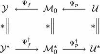(78).

  

  (78)

  It can be discerned that duality of $\mathcal M _0$ with $\mathcal M _0 ^*$ can be attained by the alternative maps presented.

• 2. From (56a), $\hat{x}_i ^{-}(\tau )=\frac{1}{\sigma _i}Q^t\circ x_i ^{+}(t)$, thus $P^\tau \circ Q^t\circ x_i ^{+}(t)=\sigma _i^2 \,x_i ^{+}(t)$, i.e., (57a). Take (56b), $x_i ^{+}(t)=\frac{1}{\sigma _i}P^\tau \circ \hat{x}_i ^{-}(\tau )$, thus $Q^t\circ P^\tau \circ \hat{x}_i ^{-}(\tau )=\sigma _i^2 \,\hat{x}_i ^{-}(\tau )$, i.e., (57b).

• 3. From (56a) $x_i ^{+}(t)=\sigma _i Q^\tau \circ \hat{x}_i ^{-}(\tau )$ in (56b) yields (58b). From (56b) $\hat{x}_i ^{-}(\tau )=\sigma _i P^t\circ x_i ^{+}(t)$ in (56a) yields (58a). $\square$

 

 

Proof of Theorem 4.3

 

• 1. $(\Rightarrow )$: Let us verify the conditions in Theorem 4.2 after [29]: Since $\Sigma ^{+}$ in (1) is dissipative by assumption, the optimal control problems implied in (11)–(12) exist with state $x_{-} ^\star$ and co-state $\hat{x}_{-} ^\star$ trajectories for each $x^0 \in \mathcal M$, in the notation of Definition  2.5. Since the collection of all $\mathcal A (x^0,T)$ defines the reachable set, then $Int(\mathcal A (x^0,T)) \ne \emptyset , \forall x^0 \in \mathcal M$ (possibly zero though) and after Definition 4.1, we may assert that the system is weakly controllable and the support of $S_r(x^0,r)$ is the reachable set. Since after the assumption that the balancing condition (20) is satisfied, as justified in Remark 3.1, each edge point of $x_{-} ^\star$ is connected to a dual edge point of $x_{+} ^\star$ by $x_{-} ^\star (0)=x_{+} ^\star (0)=x^0 \in \mathcal M _0$, then every trajectory $x_{+} ^\star$ begins from the $r$-reachable set. Now, in the notation of Definition 2.6, consider two system trajectories $\varrho (x ^0)_1 , \varrho (x^0)_2$. Assume that $\varrho (x ^0)_1$ is state indistinguishable from $\varrho (x^0)_2$, i.e., $\varrho (x^0)_1 \, I \, \varrho (x^0)_2$. Since, due to duality, each $\varrho (x ^0)_1$ is solution of one optimal control problem, $\varrho (x^0)_1 \, I \, \varrho (x^0)_2$ implies that this is only possible if $\varrho (x ^0)_1=\varrho (x^0)_2$. Though, from Definition 4.2 indistinguishability of the input-output map implies that $h(\varrho (x^0)_1) \, I \, h(\varrho (x^0)_2)$. Since from Definition  3.6 given an output $y$ we assumed that $h: \mathcal M \rightarrow \mathcal{Y }$ provides, over all the state trajectories $x(t)$ that define the output $y$, the only one that minimizes the squared norm $\Vert x(t) \Vert _{T\mathcal M } ^2 \mathop {=}\limits ^\mathrm{{def}}S_a(x^0,r_a)$. Thus the system is observable in the sense of Definition 4.2, verifying Theorem 4.2, and then $\Sigma ^{+}$ is minimal. Consider now $\Sigma _{+} ^{\dagger }$ in (44). Since for every input trajectory $\hat{y}(t) \in \mathcal{Y }^*$ after $h^{-1}: \mathcal{Y }^* \rightarrow \mathcal M ^*$ from Definition 3.6, there is only one co-state trajectory $\hat{x}(t) \in \mathcal M ^*$ for some $\hat{x}^{0}\in \mathcal M ^*$. The set denoted by $\hat{ \mathcal A }(\hat{x}^{0},T)$ defines the reachable set and for every $\hat{x}(t)$ in the set $\{g^{-1} | \hat{u}(t)=g^{-1}(\hat{x}(t)), \hat{u}(t) \in [\hat{u}(t)] \}$ there is only one output trajectory $\hat{u}(t) \in \mathcal{U }^*$ minimizing the squared norm $\Vert \hat{x}(t) \Vert _{T^* \mathcal M } ^2 \mathop {=}\limits ^\mathrm{{def}}S_r ^*(\hat{x}^0,r_r)$. Thus, any assertion for minimality of $\Sigma ^{+}$ has a dual assertion of minimality of $\Sigma _{+} ^{\dagger }$. This part of the proof is concluded by observing that the vector fields and the systems itself are by construction symmetric, see Definition  2.3, thus there is no need of assuming analyticity. Since the group property is coordinate invariant, there exist a class of diffeomorphisms, that allow for different realizations of a unique system. Conclude then that such realizations are minimal in the sense of [12]. $(\Leftarrow ):$ By contradiction, now assume $\Sigma ^{+}$ and $\Sigma _{+} ^{\dagger }$ are not minimal and not balanced. Without assuming duality in the metric spaces defined by the Hilbert manifold structure of Proposition  2.2, still any point $\hat{x}^{0}\in \mathcal M ^*$ must have a metric defined by optimal control problem (8) for $S_r ^*(\hat{x}^0,r_r)$ (and some trajectory $x_{-}^\star$), and any point $x^0 \in \mathcal M$ must have a metric defined by optimal control problem (10) for $S_a(x^0,r_a)$ (and some trajectory $x^\star _{+}$). Any other set of points are automatically discarded since they fall outside the support of such storage functions. Nevertheless, there is no way to relate both initial conditions $x^0$ and $\hat{x}^{0}$ and thus, there may exist incomplete semi trajectories $x_{-} ^\star$ and $x_{+} ^\star$ since there is no duality to observe in Remark 3.1.

• 2. $(\Rightarrow )$: By duality in Remark 3.1, every semi trajectory $x_{+} ^* \in \mathcal M$ solution of the system $\Sigma ^{+}$ has an associated dual semi trajectory $\hat{x}_{-} ^* \in \mathcal M ^*$ solution of the adjoint system $\Sigma _{+}^{\dagger }$ and moreover every weak controllable semi trajectory $x_{-} ^*$ of $\Sigma$ is an observable semi trajectory $x_{-} ^*$ of $\Sigma ^{\dagger }$ and vice versa. Therefore the adjoint realization $\Sigma _{+}^{\dagger }$ must preserve in dual form the weak controllability and observability properties of $\Sigma ^+$. $(\Leftarrow ):$ By contradiction, assuming Eq. (20) or equivalently duality in Remark 3.1 is not satisfied, then there may exist incomplete semi trajectories $x_{-} ^\star$ and $x_{+} ^\star$ with arbitrary initial conditions $x^0$ and $\hat{x}^{0}$, and no assessment can be made on the properties of system $\Sigma ^{+}$ and $\Sigma _{+}^{\dagger }$. $\square$

References

Benenti S (1992) Orthogonal separable dynamical systems. In: Proceedings of the conference on differential geometry and its applications, pp 163–184, Opava, Czechoslovakia
Benenti S (2004) Separability on Riemannian manifolds. http://www2.dm.unito.it/simbenenti/ (unpublished)
Browder FE (1967) Nonlinear eigenvalue problems and Galerkin approximations. Bull. Am. Math Soc. 74:651–656
Clément Ph, Heijmans HJAM (1987) One-parameter semigroups. CWI Monographs 5. North Holland, Amsterdam
Curtain RF, Zwart HJ (1995) An introduction to infinite-dimensional linear systems theory. In: Texts in applied mathematics, vol 21. Springer, USA
Delaleau E, Respondek W (1995) Lowering the orders of derivatives of controls in generalized state space systems. J Math Syst Estim Control 5(3):375–378
Elkin VI (1999) Reduction of nonlinear control systems: a differential geometric approach. In: Mathematics and its applications, vol 472. Kluwer Academic, Dordrecht
Fujimoto K, Scherpen JMA (Jan. 2005) Nonlinear input-normal realizations based on the differential eigenstructure of Hankel operators. IEEE Trans Autom Control 50(1):2–18
Fujimoto K, Scherpen JMA, Gray WS (2002) Hamiltonian realizations of nonlinear adjoint operators. Automatica 38:1769–1775
Graham GE (1983) Differentiable semigroups. In: Hofmann KH, Jürgensen H, Weinert HJ (eds) Recent developments in the algebraic, analytical and topological theory of semigroups. Lecture notes in mathematics, vol 998. Springer, Berlin, pp 57–127
Gray WS, Scherpen JMA (2005) Hankel singular value functions from Schmidt pairs for nonlinear input–output systems. Syst Control Lett 54:135–144
Hermann R, Krener AJ (1977) Nonlinear controllability and observability. IEEE Trans Autom Control 22(5):728–740
Hofmann KH, Lawson JD (1983) Foundations of Lie semigroups. In: Hofmann KH, Jürgensen H, Weinert HJ (eds) Recent developments in the algebraic, analytical and topological theory of semigroups. Lecture notes in mathematics, vol 998. Springer, Berlin, pp 128–201
Hilgert J, Neeb KH (1993) Basic theory of Lie-semigroups and applications. In: Lecture notes in mathematics, vol 1552. Springer, Berlin
Jurdjevic V, Sussmann HJ (1972) Control systems on Lie groups. J Differ Equ 12:313–329
Jurdjevic V (1997) Geometric control theory. In: Studies in advanced mathematics, vol 51. Cambridge University Press, Cambridge
Lopezlena R, Scherpen JMA (2006) Energy functions for dissipativity-based balancing of discrete-time nonlinear systems. Math Control Signs Syst 18:345–368
Lopezlena R, Scherpen JMA (2006) Nonlinear behavioral balancing by extension of Lie semigroups. In: Proceedings of the 3rd IFAC workshop on Lagrangian and Hamiltonian methods for nonlinear control, Nagoya, Japan
Mirotin A (2001) On the extension of finite-dimensional representations of Lie-semigroups. Vestsi Nats Akad Navuk Belarusi Ser Fiz-Mat Navuk 140(1):18–21
Moore BC (1981) Principal components analysis in linear systems: controllability, observability, and model reduction. IEEE Trans Autom Control AC 26(1):17–32
Nijmeijer H, van der Schaft AJ (1990) Nonlinear dynamical control systems. Springer, USA
Olver PJ (1993) Applications of Lie groups to differential equations. In: Graduate texts in mathematics, 2nd edn, vol 107. Springer, USA
Palais RS, Terng C (1988) Critical point theory and submanifold geometry. In: Lecture notes in mathematics, vol 1353. Springer, USA
Polderman JW, Willems JC (1998) Introduction to mathematical systems theory: a behavioral approach. In: Texts in applied mathematics, vol 26. Springer, USA
Scherpen JMA (1993) Balancing for nonlinear systems. Syst Control Lett 21:143–153
Scherpen JMA, Gray WS (2000) Minimality and local state decompositions of a nonlinear state space realization using energy functions. IEEE Trans Autom Control AC 45(11):2079–2086
Sontag ED (1998) Mathematical control theory: deterministic finite dimensional systems. In: Texts in applied mathematics, 2nd edn, vol 6. Springer, USA
Sussmann HJ (1972) Controllability of nonlinear systems. J Differ Equ 12:95–116
Sussmann HJ (1977) Existence and uniqueness of minimal realization of nonlinear systems. Math Syst Theory 10:263–284
Weiland S (1994) A behavioral approach to balanced representations of dynamical systems. Lin Algebr Appl 205–206:1227–1252
Willems JC (1972) Dissipative dynamical systems, part 1: general theory. Arch Ration Mech Anal 45:321–351
Wonham WM (1985) Linear multivariable control: a geometric approach, 3rd edn. Springer, New York
Acknowledgments
The author gratefully acknowledges his Ph.D. advisor Prof. Dr. Ir. J.M.A. Scherpen at RUG, for her kind permission to publish the author’s research presented in this two-parts paper.
Author information
Authors and Affiliations
Corresponding author
Additional information
Enrolled as promovendus at the Delft Center for Systems and Control, Delft University of Technology, Mekelweg 2, 2628 CD Delft, The Netherlands.