A Baby Step–Giant Step Roadmap Algorithm for General Algebraic Sets

Abstract

Let $\mathrm {R}$ be a real closed field and $\mathrm{D}\subset \mathrm {R}$ an ordered domain. We present an algorithm that takes as input a polynomial $Q \in \mathrm{D}[X_{1},\ldots ,X_{k}]$ and computes a description of a roadmap of the set of zeros, $\mathrm{Zer}(Q,\,\mathrm {R}^{k}),$ of Q in $\mathrm {R}^{k}.$ The complexity of the algorithm, measured by the number of arithmetic operations in the ordered domain $\mathrm{D},$ is bounded by $d^{O(k \sqrt{k})},$ where $d = \deg (Q)\ge 2.$ As a consequence, there exist algorithms for computing the number of semialgebraically connected components of a real algebraic set, $\mathrm{Zer}(Q,\,\mathrm {R}^{k}),$ whose complexity is also bounded by $d^{O(k \sqrt{k})},$ where $d = \deg (Q)\ge 2.$ The best previously known algorithm for constructing a roadmap of a real algebraic subset of $\mathrm {R}^{k}$ defined by a polynomial of degree d has complexity $d^{O(k^{2})}.$

Appendix: Computing the Limit of Bounded Points and Curve Segments

1.1 Limit of a Bounded Point

Before computing the limit of a bounded point we need to explain how to perform some useful computations modulo a quasi-monic triangular Thom encoding $\mathcal {F},\,\sigma$ representing a point $t\in \mathrm {R}^{m}.$

We associate to $t\in \mathrm {R}^{m}$ specified by a triangular Thom encoding $\mathcal {F},\,\sigma ,$

$$\begin{aligned} {\mathcal {F}}=\left( f_{[1]},\ldots ,f_{[m]}\right) ,\quad f_{[i]}\in \mathrm{D}\left[ T_{1},\ldots ,T_{i}\right] , \end{aligned}$$

the ordered domain $\mathrm{D}[t]$ contained in $\mathrm {R}$ and generated by t.

We now aim at describing the pseudo-inverse of a nonzero element in the domain $\mathrm{D}[t]$ specified by $\mathcal {F},\,\sigma .$

Definition 8.1

A pseudo-inverse of $f\in \mathrm{D}[t]$ is an element $g\in \mathrm{D}[t]$ such that $f g\in \mathrm{D}$ is strictly positive.

This notion is delicate because the computation of the pseudo-inverse sometimes requires us to update the quasi-monic triangular Thom encoding specifying t, in the spirit of dynamical methods in algebra (e.g., [7]). We start with a motivating example.

Example 8.2

We consider t, specified as the root of

$$\begin{aligned} f(T)=T^{4}-T^{2}-2, \end{aligned}$$

giving signs $(+,\,+,\,+,\,+)$ to the set $\mathrm{Der}(f)$ of derivatives of f.

Consider $T^{2}+1.$ It is easy to see, using, for example, [2], Algorithm 10.13 (Sign Determination Algorithm)] applied to f and the list $\mathrm{Der}(f),\,T^{2}+1,$ that the sign of $T^{2}+1$ at t is positive. To compute its pseudo-inverse, we perform [2], Algorithm 8.22 (Extended Signed Subresultant)] of f and $T^{2}+1.$ If $f(T)$ and $T^{2}+1$ were coprime, we would obtain the pseudo-inverse of $T^{2}+1$ modulo $f(T)$ since the last subresultant would be a nonzero constant in $\mathrm{D}.$ But $f(T)$ and $T^{2}+1$ are not coprime and their greatest common divisor (gcd) is $T^{2}+1.$ So we divide $f(T)$ by $T^{2}+1,$ obtain a new polynomial $g(T)=T^{2}-2$, and check that the root t of $f(T)$ giving signs $(+,\,+,\,+,\,+)$ to the set $\mathrm{Der}(f)$ coincides with $\sqrt{2}$, which is the root of $T^{2}-2$, making the derivative $g^{\prime }(T)=2T$ positive, using again, for example, [2], Algorithm 10.13 (Sign Determination Algorithm)]. It is now possible to compute a pseudoreduction of $T^{2}+1$ modulo $g(T),$ which gives 3.

In other words, during the process of computing the pseudo-inverse of $T^{2}+1$, we discovered the factor $g(T)$ of $f(T)$ having t as a root and coprime with $T^{2}+1.$ Using this new description of t we were able to compute a pseudo-inverse of $T^{2}+1.$

We can now describe the computation of the pseudo-inverse in general.

Description 8.3

Given $t=(t_{1},\ldots ,t_{m}) \in \mathrm {R}^{m}$ specified by the quasi-monic triangular Thom encoding $\mathcal {F}=(f_{[1]},\ldots ,f_{[m]}),\,\sigma =(\sigma _{1},\ldots ,\sigma _{m}),$ we describe how to compute a pseudo-inverse of a nonzero element of $\mathrm{D}[t].$

We proceed by induction on the number $m$ of variables of $\mathcal {F}.$

If $m=0,$ there is nothing to do since $\mathrm{D}$ is an ordered domain.

If $m\not = 0,$ then let $t^{\prime }=(t_{1},\ldots ,t_{m-1})$ specified by $\mathcal {F}^{\prime }=(f_{[1]},\ldots ,f_{[m-1]}),\,\sigma =(\sigma _{1},\ldots ,\sigma _{m-1}).$

We consider f a polynomial in $T_{m}$ whose coefficients, which are elements of

$$\begin{aligned} \left\{ h\in \mathrm{D}\left[ T_{1},\ldots ,T_{m-1}\right] \mid \deg _{T_{i}}(h)<\deg _{T_{i}}\left( f_{[i]}\right) ,\, i=1,\ldots ,m-1\right\} , \end{aligned}$$

represent elements of $\mathrm{D}[t^{\prime }].$

We first decide the sign of f at t, which is done by [2], Algorithm 12.19 (Triangular Sign Determination Algorithm)].

If $f(t)\not =0,$ then we try to pseudo-invert f modulo $\mathcal {F}.$ We perform [2], Algorithm 8.22 (Extended Signed Subresultant)] for f and $f_{[m]},$ with respect to the variable $T_{m}$, and compute a $\gcd (f,\,f_{[m]})\in \mathrm{D}[t^{\prime }]$ (the last nonzero subresultant polynomial) as well as the cofactors $u,\,v\in \mathrm{D}[t^{\prime }]$ with $uf+vf_{[m]}=\gcd (f,\,f_{[m]}).$

• (1) If $\gcd (f,\,f_{[m]})$ is of degree 0 in $T_{m}$, then $u$ is a quasi-inverse of f.

• (2) If $\gcd (f,\,f_{[m]})$ is of degree $>$0 in $T_{m}$, then we have discovered a factor of $f_{[m]}.$ We define h as the quasi-monic polynomial proportional to $f_{[m]}/\gcd (f,\,f_{[m]})$ obtained by [2], Algorithm 8.22 (Extended Signed Subresultant)] (see [2], Algorithm 10.1 (Gcd and Gcd-free part)]). We perform [2], Algorithm 12.19 (Triangular Sign Determination)] applied to $f_{[m]}$ and $\mathrm{Der}(f_{[m]}),\,\mathrm{Der}(h)$ to identify the Thom encoding $\tau$ of $t_{[m]}$ as a root of h. We replace $f_{[m]}$ with h and $\sigma _{[m]}$ with $\tau$ in $\mathcal {F}.$ Now f and the new $f_{[m]},$ considered as polynomials in $T_{[m]}$, are coprime, and we can invert f modulo $f_{[m]}.$

Proposition 8.4

Let $\mathrm{D}$ be an ordered domain contained in a real closed field $\mathrm {R},$ and let $t=(t_{1},\ldots ,t_{m})\in \mathrm {R}^{m}$ be specified by a quasi-monic triangular Thom encoding $\mathcal {F},\,\sigma ,$

$$\begin{aligned} \mathcal {F}=\left( f_{[1]},\ldots ,f_{[m]}\right) ,\quad f_{[i]}\in \mathrm{D}\left[ T_{1},\ldots ,T_{i}\right] . \end{aligned}$$

Let d be a bound of the degree of $f_{[i]}$ with respect to each $T_{j},\,1\le j\le i,\,1\le i\le m.$

• (a) If $g\in \mathrm{D}[T_{1},\ldots ,T_{m}]$ is a polynomial of degree $D,$ then the complexity of computing a pseudoreduction $(c,\,\bar{g})$ of g modulo $\mathcal {F}$ is $(D d)^{O(m)}$ arithmetic operations in $\mathrm{D}.$

• (b) The complexity of the computation of the pseudo-inverse of an element of $\mathrm{D}[t]$ is $d^{O(m)}$ arithmetic operations in $\mathrm{D}.$

Proof

(a) Suppose that $C_{g}\in \mathrm{D}$ is such that $C_{g} T_{1}^{i_1}\cdots T_{m}^{i_{m}} g$ has a reduction in $\mathrm{D}$ modulo $\mathcal {F}$ for every $(i_{1}, \ldots i_{m})$, with $i_{j}<\mathrm{deg}(f_{[j]},\,T_{j}),\,1\le j\le m.$ We denote by $\mathrm{Mat}(C_{g} g)$ the matrix of multiplication by $C_{g} g$ modulo $(\mathcal {F})$ with respect to monomial bases. The entries of $\mathrm{Mat}(C_{g} g)$ are in $\mathrm{D}.$ Its rows and columns are indexed by $(i_{1}, \ldots , i_{m}),\,i_{j}<\mathrm{deg}(f_{[j]},\,T_{j}),\,1\le j\le m$, and the $(j_{1},\ldots ,j_{m})$th entry of the column indexed by $(i_{1},\ldots ,i_{m})$ is the coefficient of $T_{1}^{j_{1}}\cdots T_{m}^{j_{m}}$ in the reduction of $C_{g} T_{1}^{i_{1}}\cdots T_{m}^{i_{m}} g$ modulo $\mathcal {F}.$ Note that $\mathrm{Mat}(C_{g} C_{h} gh)=\mathrm{Mat}(C_{g} g)\mathrm{Mat}(C_{h} h).$ Note also that the entries of the first column of $\mathrm{Mat}(C_{g} g)$ [indexed by $(0,\ldots ,0)$] are the coefficients of the reduction of $C_{g} g$ modulo $\mathcal {F}.$

We first compute $C_{T_{j}}$ such that $C_{T_{j}} T_{1}^{i_{1}}\cdots T_{m}^{i_{m}} T_{j}$ has a reduction in $\mathrm{D}$ modulo $\mathcal {F}$ for every $(i_{1}, \ldots i_{m}),\,i_{h}<\mathrm{deg}(f_{[h]},\,T_{h}),\,1\le h\le m.$ The algorithm proceeds by induction on j.

For $j=1,$ let $c_{1}\in \mathrm{D}$ be the leading coefficient of $f_{[1]}\in \mathrm{D}[T_{1}],\,d_{1}=\mathrm{deg}(f_{[1]},\,T_1),$ and let $C_{T_1}=c_{1}.$ The matrix $\mathrm{Mat}(c_{1} T_{1})$ is simply obtained by replacing each occurrence of $c_{1} T_{1}^{d_{1}}$ by $f_{[1]}-c_{1}T_{1}^{d_{1}}$ in

$$\begin{aligned} c_1 T_1^{d_1-1} T_{2}^{i_2}\cdots T_{m}^{i_m} T_1, \end{aligned}$$

with $i_h<d_h,\,2\le h\le m$ and writing the result as a linear combination of the monomials $T_{1}^{j_1}\cdots T_{m}^{j_m},\,j_i<d_i,\,1\le i \le m.$ Compute $\mathrm{Mat}(C_{T_1}^{h} T_1^{h})=\mathrm{Mat}(c_1 T_1)^{h},\,h<2d,$ and define $C_1=c_1^{2d-1}.$

Suppose by induction that for every monomial M in $T_1,\ldots , T_j$ of degree $<$2d, $C_M T_1^{i_1}\cdots T_m^{i_m} M$ has a reduction in $\mathrm{D}$ modulo $\mathcal {F}$ for every $(i_1, \ldots , i_m),\,i_j<\mathrm{deg}(f_{[j]},\,T_j),\,1\le j \le m.$ Also, suppose that $\mathrm{Mat}( C_{M} M)$ has been computed. Denote by $C_{j}\in \mathrm{D}$ the product of $C_M$ for all the monomials M of degree $<$2d in the j variables $T_1,\ldots ,T_j.$

Let $c_{j+1}\in \mathrm{D}$ be the leading coefficient of $f_{[j+1]}\in \mathrm{D}[T_1,\ldots ,T_{j+1}]$ with respect to $T_{j+1}$ and $d_{j+1}=\mathrm{deg}(f_{[j+1]},\,T_{j+1}),$ and take $C_{T_{j+1}}=c_{j+1} C_{j}.$ The matrix $\mathrm{Mat}(C_{T_{j+1}} T_{j+1})$ is obtained by replacing each occurrence of $C_{T_{j+1}} T_{j+1}^{d_{j+1}}$ by $C_{j}f_{[j+1]}-C_{T_{j+1}} T_{j+1}^{d_{j+1}}$ in

$$\begin{aligned} C_{T_{j+1}} T_{1}^{i_1}\cdots T_{j}^{i_j}T_{j+1}^{d_{j+1}-1}T_{j+2}^{i_{j+2}}\cdots T_{m}^{i_m} T_{j+1}, \end{aligned}$$

with $i_\ell <d_\ell .$

Notice that the polynomials obtained in this way have degrees at most $2d$ in $T_1,\ldots ,T_j$ and degrees $<d_h$ in $T_h$ for $h > j.$ Reduce all such monomials using the matrices of multiplication computed previously.

Finally, compute for every monomial M of degree $\le D$, in $T_1,\ldots ,T_m,\,C_M$ and $\mathrm{Mat}(C_{M} M)$ by taking products of the $C_{T_i}$ and the matrices $\mathrm{Mat}(C_{T_i} T_i)$ (respectively), and let $C_g$ be the product of the $C_M$ for all monomials M of degree $\le D.$ Now determine $\mathrm{Mat}(C_{g} g)$ by taking an appropriate linear combination of $\mathrm{Mat}(C_{M} M)$ and in that way obtain the reduction of $C_g g$ modulo $\mathcal {F}.$

Notice that the complexity of computing the $C_{T_{j+1}}$ and $\mathrm{Mat}(C_{T_{j+1}} T_{j+1})$ is bounded by $d^{O(m)}.$ In the last step, there are $O(D)^m$ monomials of degree at most D, and hence at most $O(D)^m$ matrix multiplications to perform, and the sizes of the matrices are $d_1\cdots d_m \le d^m.$ Thus, the complexity is $(Dd)^{O(m)}.$

(b) The proof proceeds by induction on the number of variables m of ${\mathcal {F}}.$

If $m=1,$ then the computation of a gcd takes $(d+1)^{c}$ operations in the domain $\mathrm{D},$ for some universal constant $c > 0,$ using the complexity analysis of [2], Algorithm 8.22 (Extended Signed Subresultant)] and [2], Algorithm 10.13 (Sign Determination)].

If $m>1$, let $t=(t^{\prime },\,u),$ and we suppose by the induction hypothesis that the complexity of arithmetic operations including pseudo-inverse in $\mathrm{D}[t^{\prime }]$ is $(d+1)^{c(m-1)}$ arithmetic operations in the ordered domain $\mathrm{D}.$ The claim is clear since the arithmetic operations in the domain $\mathrm{D}[t]$ use $(d+1)^{c}$ operations in the domain $\mathrm{D}[t^{\prime }]$ using the complexity analysis of [2], Algorithm 8.22 (Extended Signed Subresultant)] and [2], Algorithm 10.13 (Sign Determination)]. $\square$

We can now give the description of Algorithm 3 (Limit of a Bounded Point).

Description of Algorithm 3 (Limit of a Bounded Point)

The precise input and output of this algorithm appear in Sect. 6.2.

Procedure Remove from $g(\varepsilon )(T_1,\ldots ,T_m,\,U)$ the coefficients vanishing at the point $(t_1,\ldots ,t_m)$ using [2], Algorithm 12.19 (Triangular Sign Determination)]. Supposing without loss of generality that not all the coefficients of

$$\begin{aligned} g(\varepsilon )\left( t_1,\ldots ,t_m,\,U\right) \end{aligned}$$

are multiples of $\varepsilon ,$ denote by $g(T_1,\ldots ,T_m,\,U)$ the polynomial obtained by substituting $0$ for $\varepsilon$ in $g(\varepsilon )(T_1,\ldots ,T_m,\,U).$

Similarly, denote by $G(T_1,\ldots ,T_m,\,U)$ the polynomials obtained by substituting $0$ for $\varepsilon$ in $G(\varepsilon )(T_1,\ldots ,T_m,\,U).$

Compute the set $\varSigma$ of Thom encodings of roots of $g(t,\,U)$ using [2], Algorithm 12.19 (Triangular Sign Determination)]. Denoting by $\mu _\sigma$ the multiplicity of the root of $g(t,\,U)$ with Thom encoding $\sigma ,$ define $G_\sigma$ as the $(\mu _\sigma -1)$th derivative of G with respect to U.

Identify the Thom encoding $\sigma$ and $G_\sigma$ representing z, using [2], Algorithm 12.19 (Triangular Sign Determination)], by checking whether a ball of infinitesimal radius $\delta$ ($1\gg \delta \gg \varepsilon >0$) around the point x represented by the real univariate representation $g,\,\sigma ,\,G_\sigma$ contains $z(\varepsilon ).$

Pseudo-invert the leading coefficient of the univariate representation, denote by $\mathcal {F}^{\prime },\,\sigma ^{\prime }$ the new triangular Thom encoding describing $t$, and compute a pseudoreduction of the output modulo $\mathcal {F}^{\prime }.$

Complexity analysis follows from the complexity of [2], Algorithm 12.19 (Triangular Sign Determination)].

1.2 Limit of a Curve

Computing the limit of a curve is not immediate when some part of the curve has a vertical limit, as seen in the following example.

Example 8.5

Consider the s-a curve $\gamma :\,[0,\,\varepsilon ]\rightarrow \mathrm {R}\langle \varepsilon \rangle ^3,$ parametrized by the $X_1$-coordinate defined by

$$\begin{aligned} \gamma \left( x_1\right) = \left( x_1,\,\gamma _2\left( x_1\right) ,\,\gamma _3\left( x_1\right) \right) ,\quad x_1 \in [0,\,\varepsilon ], \end{aligned}$$

where $(\gamma _2(x_1),\,\gamma _3(x_1))$ is the solution of the triangular system

$$\begin{aligned} X_2 - x_1/\varepsilon = 0, \\ X_2^2 + X_3^2 - 1 = 0, \end{aligned}$$

with Thom encoding $(0,\,+),\,(0,\,+,\,+).$

Notice that the image of $\gamma$ is contained in the cylinder of unit radius, with the $X_1$-axis as the axis, and is bounded over $\mathrm {R}.$ The image of $\gamma$ under the $\lim _\varepsilon$ map is contained in a circle in the plane $X_1=0$ and can no longer be described as a curve parametrized by the $X_1$-coordinate.

However, it is possible to reparametrize $\gamma$ by the $X_2$-coordinate. In doing so we obtain another s-a curve $\varphi :\,[0,\,1] \rightarrow \mathrm {R}\langle \varepsilon \rangle ^3$ (having the same image as $\gamma$) defined by

$$\begin{aligned} \varphi \left( x_2\right) = \left( \varphi _1\left( x_2\right) ,\,x_2,\,\varphi _3\left( x_2\right) \right) ,\quad x_2 \in [0,\,1], \end{aligned}$$

where $(\varphi _1(x_2),\,\varphi _3(x_2))$ is the real solution of the triangular system

$$\begin{aligned} X_1-\varepsilon x_2 = 0, \\ X_3^2 + x_2^2 - 1 = 0, \end{aligned}$$

with Thom encoding $(0,\,-),\,(0,\,+,\,+).$ Notice that the image under $\lim _\varepsilon$ of the curve that is the graph of $\varphi$ can be easily described as the curve represented by the following triangular system parametrized by $x_2 \in [0,\,1]$:

$$\begin{aligned} X_1 = 0, \\ X_3^2 + x_2^2 - 1 = 0, \end{aligned}$$

and Thom encoding $(0,\,-1),\,(0,\,+,\,+).$

This is why some kind of reparametrization is necessary before computing the limit.

1.2.1 Reparametrization of Curve Segments

We define the notion of a well-parametrized curve and prove that the limit of a well-parametrized curve is easy to describe.

Definition 8.6

A differentiable s-a curve

$$\begin{aligned} \gamma = \left( \gamma _1,\ldots ,\gamma _k\right) :\,(a,\,b)\rightarrow \mathrm {R}^k, \end{aligned}$$

parametrized by $X_1$ [i.e., $\gamma _1(x_1)=x_1$] is well parametrized if for every $x_1 \in (a,\,b)$

$$\begin{aligned} \sum _{i=1}^k \left( \frac{\partial \gamma _i}{\partial X_1}\right) ^2 \le k. \end{aligned}$$

Let $t\in \mathrm {R}^m$ be represented by a triangular Thom encoding $\mathcal {F},\,\sigma$, and let

$$\begin{aligned} f_1,\,\sigma _1,\, f_2,\, \sigma _2,\,g,\, \tau ,\,G \end{aligned}$$

be a curve segment with parameter $X_j$ over t on $(\alpha _1,\,\alpha _2)$, where $\alpha _1$ and $\alpha _2$ are the elements of $\mathrm {R}$ represented by the Thom encodings $f_1,\,\sigma _1$ and $f_2,\,\sigma _2.$

The curve segment

$$\begin{aligned} f_1,\,\sigma _1,\, f_2,\, \sigma _2,\,g,\, \tau ,\,G \end{aligned}$$

is well parametrized if the s-a curve $\gamma :\,(\alpha _1,\,\alpha _2)\rightarrow \mathrm {R}\langle \varepsilon \rangle ^k$ defined by

$$\begin{aligned} \gamma \left( x_j\right) = \left( \frac{g_{1} (t,\,x_j,\, u(x_j))}{g_0 (t,\,x_j,\,u(x_j))}, \ldots , \frac{g_k (t,\,x_j,\, u(x_j))}{g_0 (t,\,x_j,\, u(x_j))} \right) , \end{aligned}$$

is well parametrized, where $u:\,(\alpha _1,\,\alpha _2) \rightarrow \mathrm {R}$ maps each $x_j \in (\alpha _1,\,\alpha _2)$ to the root of $g(t,\,x_j,\,U)$ with Thom encoding $\tau .$ This means that

$$\begin{aligned} \sum _{i=1}^k\left( \left( \frac{g_i (t,\,x_j,\,u(x_j))}{g_0 (t,\,x_j,\,u(x_j))} \right) ^{\prime }\right) ^2 \le k, \end{aligned}$$

where the derivative is taken with respect to $x_j.$

Example 8.5 is not a well-parametrized curve segment.

If a curve segment defined over $\mathrm {R}\langle \varepsilon \rangle$ is well parametrized and represents a curve bounded over $\mathrm {R},$ then the image of the curve under the $\lim _\varepsilon$ map can be easily described. The following proposition explains why this is true.

Proposition 8.7

Let $(a(\varepsilon ),\,b(\varepsilon ))\subset \mathrm {R}\langle \varepsilon \rangle ,\,a(\varepsilon ),\,b(\varepsilon )$ be bounded over $\mathrm {R},\,r < j \le k,\,z(\varepsilon ) \in \mathrm {R}\langle \varepsilon \rangle ^{r},$ and let

$$\begin{aligned} \gamma (\varepsilon ) =:(a(\varepsilon ),\,b(\varepsilon ))\rightarrow \{z(\varepsilon )\} \times \mathrm {R}\langle \varepsilon \rangle ^{k - r} \end{aligned}$$

be a s-a differentiable curve parametrized by $X_j$ and bounded over $\mathrm {R}.$ If $\gamma (\varepsilon )$ is well parametrized, then:

• (1) There exists a continuous extension of $\gamma (\varepsilon )$ to a continuous s-a curve,

  $$\begin{aligned} \gamma (\varepsilon ) = :[a(\varepsilon ),\,b(\varepsilon )] \rightarrow \{z(\varepsilon )\} \times \mathrm {R}\langle \varepsilon \rangle ^{k - r}, \end{aligned}$$

  defined over the closed interval $[a(\varepsilon ),\,b(\varepsilon )]$;

• (2) For each $x \in [\lim _\varepsilon ( a(\varepsilon )),\,\lim _\varepsilon (b(\varepsilon ))]$ and any $x(\varepsilon ) \in [a(\varepsilon ),\,b(\varepsilon )]$, with $\lim _\varepsilon (x(\varepsilon )) = x,\,\gamma (x):=\lim _\varepsilon (\gamma (\varepsilon )(x)) = \lim _\varepsilon (\gamma (\varepsilon )(x(\varepsilon )))$;

• (3) $\lim _\varepsilon (\gamma (\varepsilon )([a(\varepsilon ),\,b(\varepsilon )])) = \gamma ([\lim _\varepsilon (a(\varepsilon )),\,\lim _\varepsilon (b(\varepsilon ))]).$

In other words, the graph of the s-a function $\gamma (-):= \lim _\varepsilon (\gamma (\varepsilon )(-))$ is the image under $\lim _\varepsilon$ of the graph of $\gamma (\varepsilon ).$

Proof

Since $\gamma (\varepsilon )$ is bounded, it follows that there exists a continuous extension of $\gamma (\varepsilon )$ to the endpoints of the interval $(a(\varepsilon ),\,b(\varepsilon )).$ It also follows from the definition of being well parametrized that $||\gamma (\varepsilon )^{\prime }(x)|| \le \sqrt{k}$ for all $x\in (a(\varepsilon ),\,b(\varepsilon )).$ By the s-a mean value theorem [2], Exercice 3.4], we have that for each $x \in (a(\varepsilon ),\,b(\varepsilon ))\cap \mathrm {R}$ and any $x(\varepsilon ) \in (a(\varepsilon ),\,b(\varepsilon ))$, with $\lim _\varepsilon ( x(\varepsilon )) = x,$

$$\begin{aligned} ||\gamma (\varepsilon )(x) - \gamma (\varepsilon )(x(\varepsilon ))|| =||\gamma (\varepsilon )^{\prime }(w(\varepsilon ))|||x-x(\varepsilon )| \end{aligned}$$

for some $w \in (x,\,x(\varepsilon ))$ [assuming without loss of generality that $x < x(\varepsilon )$]. Taking the image under $\lim _\varepsilon$ and noticing that $||\gamma (\varepsilon )^{\prime }(w(\varepsilon ))||$ is bounded over $\mathrm {R}$ by the previous observation, we obtain that

$$\begin{aligned} \lim _\varepsilon (\gamma (\varepsilon )(x)) = \lim _\varepsilon (\gamma (\varepsilon )(x(\varepsilon ))), \end{aligned}$$

proving (1). This implies that the function $\gamma :\,(\lim _\varepsilon (a(\varepsilon )),\,\lim _\varepsilon (b(\varepsilon ))) \rightarrow \mathrm {R}^k$ defined by $\gamma (x) = \lim _\varepsilon (\gamma (\varepsilon )(x))$ is a continuous, bounded [since $\gamma (\varepsilon )$ is bounded over $\mathrm {R}$] s-a function and, hence, can be extended to a continuous, bounded s-a function on the closed interval $[\lim _\varepsilon ( a(\varepsilon )),\,\lim _\varepsilon (b(\varepsilon ))].$ Moreover, it is clear that $\gamma (\lim _\varepsilon (a(\varepsilon ))) = \lim _\varepsilon (\gamma (\varepsilon )(a(\varepsilon )))$ and $\gamma (\lim _\varepsilon (b(\varepsilon ))) = \lim _\varepsilon (\gamma (\varepsilon )(b(\varepsilon )))$ since

$$\begin{aligned} \gamma (\lim _\varepsilon (a(\varepsilon ))),\,\gamma (\lim _\varepsilon (b(\varepsilon ))) \in \overline{\gamma ((\lim _\varepsilon (a(\varepsilon )),\,\lim _\varepsilon (b(\varepsilon ))))}=\lim _\varepsilon (\gamma (\varepsilon )([a(\varepsilon ),\,b(\varepsilon )])). \end{aligned}$$

It is then clear that (2) follows.

A s-a curve is in general not well parametrized. However, subdividing if necessary the curve into several pieces, it is possible to choose for each such piece a parametrizing coordinate that makes the piece well parametrized. This is what we do in Algorithm 8 (Reparametrization of a Curve).

Proof of correctness. Let

$$\begin{aligned} \left( f_1,\,\sigma _1,\,f_2,\,\sigma _2,\,g,\, \tau ,\,G\right) \end{aligned}$$

be a curve segment parametrized by $X_1$ over t representing the curve $\gamma :\,(a,\,b) \rightarrow \mathrm {R}^k.$

Let $(c,\,d)$ be a subinterval of $(a,\,b)$ such that for every $x_1\in (a,\,b)$

$$\begin{aligned} G_\ell \left( t,\,x_1,\,u\left( x_1\right) \right) = k F_\ell ^2\left( t,\,x_1,\,u\left( x_1\right) \right) - \sum _{j=1}^{k}F_j^2\left( t,\,x_1,\,u\left( x_1\right) \right) \ge 0 \end{aligned}$$

(8.1)

(using the notation of Steps 1 and 2).

This implies

$$\begin{aligned} \left| \frac{\partial \gamma _\ell }{\partial X_1} \right| \ge \frac{1}{\sqrt{k}}, \end{aligned}$$

and hence the mapping $\gamma _\ell$ from $(c,\,d)$ to $(c^{\prime },\,d^{\prime })$, with $c^{\prime }=\gamma _\ell (c),\,d^{\prime }=\gamma _\ell (d)$, is invertible. Defining $\bar{\gamma }(x_\ell )=\gamma (\gamma _\ell ^{-1}(x_\ell )),\,\bar{\gamma }((c^{\prime },\,d^{\prime }))=\gamma ((c,\,d))$ is well parametrized by $X_\ell .$

Moreover, at each point $x_1 \in (a,\,b)$ such a choice of $\ell$ exists since there must exist an $\ell ,\, 1 \le \ell \le k$ such that $\displaystyle {\left( \frac{\partial \gamma _\ell }{\partial X_1}\right) ^2}$ is at least the average value $\displaystyle {\frac{1}{k}\sum \nolimits _{i=1}^k \left( \frac{\partial \gamma _i}{\partial X_1}\right) ^2}.$ Notice also that for such a choice of $\ell$ we have, by the chain rule,

$$\begin{aligned} \sum _{i=1}^k \left( \frac{\partial \gamma _i}{\partial X_\ell }\right) ^2 = \frac{\sum _{i=1}^k \left( \frac{\partial \gamma _i}{\partial X_1}\right) ^2}{\left( \frac{\partial \gamma _\ell }{\partial X_1}\right) ^2}\le k. \end{aligned}$$

(8.2)

In Step 2 of the algorithm we obtain a partition of the interval $(a,\,b)$ into points and open intervals such that over each subinterval $(c_{j-1},\,c_j)$ of the partition there exists an index $\ell = \ell (j)$ such that (8.1) is satisfied at each point $v \in (c_{j-1},\,c_j),$ and the curve segment over this interval is well parametrized by $X_\ell$ by (8.2).

Each curve segment corresponding to elements of $\mathcal {V}$ output by the algorithm is thus well parametrized. The remaining property of the output is a consequence of the correctness of Algorithm 1 (Curve Segments) and [2], Algorithm 12.19 (Triangular Sign Determination)]. $\square$

Complexity analysis. Let $\mathrm{D}$ be a bound on the degrees of the polynomials in the input. The complexity of Steps 1 and 2 is bounded by $k^{O(1)} \mathrm{D}^{O(m)}$ from the complexity of [2], Algorithm 11.19 (Restricted Elimination)] and [2], Algorithm 12.23 (Triangular Sample Points)], noting that the number of polynomials in $\mathcal {L}$ is bounded by $k^{O(1)} \mathrm{D}^{O(m)}.$

In Steps 3 and 4 Algorithm 1 (Curve Segments) and [2], Algorithm 12.19 (Triangular Sign Determination)] are both called with a constant number of variables in the input. Using the complexity analysis of these algorithms, the total complexity is bounded by $k^{O(1)} D^{O(m)}.$ $\square$

1.2.2 Limit of a Curve

We are now ready to describe Algorithm 4 (Limit of a Curve).

Description of Algorithm 4 (Limit of a Curve)

The algorithm proceeds by reparametrizing the curve and computing the limit of the well-parametrized curve segments thus obtained, as explained in what follows. Its precise input and output appear in Sect. 6.2.

Procedure.

Step 1. :

Let $T=(T_1,\ldots ,T_m),\,X^{\prime }=(X_{1},\ldots ,X_{r}).$ Call a slight variant of [2], Algorithm 12.18 (Parametrized Bounded Algebraic Sampling)], computing pseudoreductions of the intermediate computations modulo $\mathcal {F}$ (using Proposition 8.4), with input

$$\begin{aligned} \sum _{A\in \mathcal {H}(\varepsilon )}A^2\in \mathrm{D}[\varepsilon ,\,T,\,X^{\prime }] \end{aligned}$$

and parameters $\varepsilon ,\,T,$ and output the set $\mathcal {U}_{\varepsilon }$ of parametrized univariate representations with variable U. For every $(h(\varepsilon ),\,H(\varepsilon )) \in \mathcal {U}(\varepsilon ),$ use [2], Algorithm 12.20 (Triangular Thom Encoding)], with the triangular system $(\mathcal {F},\,h(\varepsilon ))$ as input, to compute the Thom encodings of the real roots of $h(\varepsilon )(y,\,U).$ If

$$\begin{aligned} \mathcal {H}(\varepsilon )=\left( h_{[1]},\ldots ,h_{[r]}\right) , \end{aligned}$$

with $h_{[i]}\in \mathrm{D}[T,\,X_1,\ldots ,X_i]$, substitute the variables $X^{\prime }$ into

$$\begin{aligned} \bigcup _{0,\ldots ,r} \mathrm{Der}_{X_i}\left( h_{[i]}\right) , \end{aligned}$$

using $H(\varepsilon )$ by Notation 4.5, and define a family $\mathcal {A}$ of polynomials in $\varepsilon ,\,T,\,U.$ Using [2], Algorithm 12 (Triangular Sign Determination)], compute the signs of the polynomials of $\mathcal {A}$ at the roots of $h(\varepsilon )(y,\,U).$ Comparing the Thom encodings, identify a specific $(h(\varepsilon ),\,\tau (\varepsilon ),\,H(\varepsilon ))$ representing $z(\varepsilon )$ over t. Then apply Algorithm 3 (Limit of a Bounded Point) with input

$$\begin{aligned} (h(\varepsilon ),\,\tau (\varepsilon ),\,H(\varepsilon )), \end{aligned}$$

representing $z(\varepsilon )$ over t, to obtain a real univariate representation $p_z,\,\rho _z,\,P_z$ representing z over t.

Step 2. :

Using Algorithm 8 (Reparametrization of a Curve), reparametrize the input curve segment.

Step 3. :

For every well-parametrized curve segment $S(\varepsilon )$ computed in Step 2 and represented by

$$\begin{aligned} \left( f(\varepsilon )_{1},\,\sigma (\varepsilon )_{1},\,f(\varepsilon )_{2},\,\sigma (\varepsilon )_{2},\,g(\varepsilon ),\,\tau (\varepsilon ),\,G(\varepsilon )\right) , \end{aligned}$$

do the following. First reorder the variables to ensure that the parameter of $S(\varepsilon )$ is $X_{r+1}.$ Then compute a description of $\lim _\varepsilon (S(\varepsilon )).$ This process will generate a finite list of open intervals and points above which the representation of the restriction of the curve $\lim _\varepsilon (S(\varepsilon ))$ by a curve segment is fixed. This is done as follows.

Step 3(a). :

Denote by $\alpha (\varepsilon )_{1}$ the element of $\mathrm {R}\langle \varepsilon \rangle$ represented by

$$\begin{aligned} f(\varepsilon )_{1}\left( T,\,X^{\prime },\,X_{r+1}\right) ,\,\sigma (\varepsilon )_{1} \end{aligned}$$

over $(t,\,z(\varepsilon )).$ Call a slight variant of [2], Algorithm 12.18 (Parametrized Bounded Algebraic Sampling)], computing a pseudoreduction of the intermediate computations modulo $\mathcal {F}$ of the output modulo $\mathcal {F}$ (using Proposition 8.4), with input

$$\begin{aligned} \sum _{A\in \mathcal {H}(\varepsilon )}A^2+f(\varepsilon )_{1}\left( T,\,X^{\prime },\,X_{r+1}\right) ^2 \in \mathrm{D}\left[ \varepsilon ,\,T,\,X^{\prime },\,X_{r+1}\right] \end{aligned}$$

and parameters $\varepsilon ,\,T,$ and output a set $\mathcal {U}^{\prime }_{\varepsilon }$ of parametrized univariate representations with variable U. For every $(h(\varepsilon ),\,H(\varepsilon )) \in \mathcal {U}^{\prime }_{\varepsilon },$ use [2], Algorithm 12.20 (Triangular Thom Encoding)], with the triangular system $(\mathcal {F},\,h(\varepsilon ))$ as input, to compute the Thom encodings of the real roots of $h(\varepsilon )(y,\,U).$ If

$$\begin{aligned} \mathcal {H}(\varepsilon )=\left( h_{[1]},\ldots ,h_{[r]}\right) , \end{aligned}$$

with $h_{[i]}\in \mathrm{D}[T,\,X_1,\ldots ,X_i],$ substitute the variables $X^{\prime },\,X_{r+1}$ into

$$\begin{aligned} \mathrm{Der}_{X_{r+1}}f(\varepsilon )_{1}\left( T,\,X^{\prime },\,X_{r+1}\right) ,\,X_{r+1}\cup \bigcup _{1,\ldots ,r} \mathrm{Der}_{X_i}\left( h_{[i]}\right) \end{aligned}$$

using Notation 4.5, and define a family $\mathcal {B}$ of polynomials in $\varepsilon ,\,T,\,U.$ Using [2], Algorithm 12 (Triangular Sign Determination)], compute the signs of the polynomials of $\mathcal {B}$ at the roots of $h(\varepsilon )(y,\,U).$ Comparing the Thom encodings, identify a specific $(h(\varepsilon ),\,\tau (\varepsilon ),\,H(\varepsilon ))$ representing $(z(\varepsilon ),\,\alpha (\varepsilon )_{1})$ over t. Then apply Algorithm 3 (Limit of a Bounded Point) with input

$$\begin{aligned} (h(\varepsilon ),\,\tau (\varepsilon ),\,H(\varepsilon )) \end{aligned}$$

representing $(z(\varepsilon ),\,\alpha (\varepsilon )_{1})$ over t to obtain a quasi-monic real univariate representation $p_{z,\alpha _1},\,\rho _{z,\alpha _1},\,P_{z,\alpha _1}$ representing $(z,\,\alpha _1)$ over t, with $\alpha _1=\lim _\varepsilon (\alpha (\varepsilon )_{1}).$ Obtain a Thom encoding over t of $\alpha _1$ using [2], Algorithm 15.1 (Projection)]. Similarly, for $\alpha (\varepsilon )_{2}$ the element of $\mathrm {R}\langle \varepsilon \rangle$ represented by

$$\begin{aligned} f(\varepsilon )_{2}\left( T,\,X^{\prime },\,X_{r+1}\right) ,\,\sigma (\varepsilon )_{2}, \end{aligned}$$

over $(t,\,z(\varepsilon )),$ compute a Thom encoding over t of $\alpha _2=\lim _\varepsilon (\alpha (\varepsilon )_{2}).$

Step 3(b). :

Perform a slight variant of [2], Algorithm 12.18 (Parametrized Bounded Algebraic Sampling)], computing pseudoreductions of intermediate computations modulo $\mathcal {F}$ of the output modulo $\mathcal {F}$ (using Proposition 8.4), with input

$$\begin{aligned} \sum _{A\in \mathcal {H}(\varepsilon )}A^2+g(\varepsilon )\left( T,\,X^{\prime },\,X_{r+1},\,V\right) ^2 \in \mathrm{D}\left[ \varepsilon ,\,T,\,X^{\prime },\,X_{r+1},\,U\right] \end{aligned}$$

and parameters $\varepsilon ,\,T,\,X_{r+1}$, and output a set $\mathcal {V}(\varepsilon )$ of parametrized univariate representations with parameter $\varepsilon ,\,T,\,X_{r+1}$ and variable V. Denote by $\mathbf {\varTheta }(\varepsilon )$ the set of polynomials $\theta (\varepsilon )$ such that there exists $\varTheta (\varepsilon )$, with $(\theta (\varepsilon ),\,\varTheta (\varepsilon ))\in \mathcal {V}(\varepsilon ).$ Note that $\theta (\varepsilon ) \in \mathrm{D}[\varepsilon ,\,T,\,X_{r+1},\,V].$

Step 3(c). :

Compute the family of coefficients $\mathcal {C}\subset \mathrm{D}[T,\,X_{r+1}]$ of the polynomials $\theta (\varepsilon ) \in \mathbf {\varTheta }(\varepsilon )$ considered as elements of $\mathrm{D}[T,\,X_{r+1}][\varepsilon ,\,V]$ and the list $\mathcal {L} \subset \{=0,\,\ne 0\}^{\mathcal {C}}$ of nonempty conditions $=0,\,\not = 0$ satisfied by $\mathcal {C}$ in $\mathrm {R}$ using [2], Algorithm 12.23 (Triangular Sample Points)]. Note that for every $x_{r+1}$ in the realization of $\tau \in \mathcal {L},$ the orders in $\varepsilon$ of the coefficients of the polynomials in $\mathbf {\Theta }(\varepsilon )(t,\,x_{r+1})\subset \mathrm{D}[\varepsilon ,\,V]$ are fixed. For every $\theta (\varepsilon ) \in \mathbf {\varTheta }(\varepsilon )$ we denote by $o(\theta (\varepsilon ),\,\tau )$ the minimal order in $\varepsilon$ of the coefficients of $\theta (\varepsilon )(t,\,x_{r+1})$ on the realization of $\tau$ and by $\mathbf {\varTheta }_\tau \subset \mathrm{D}[T,\,X_{r+1},\,V]$ the set of polynomials obtained by substituting $0$ for $\varepsilon$ in $\varepsilon ^{-o(\theta (\varepsilon ),\tau )}\theta (\varepsilon ).$

Step 3(d). :

Define

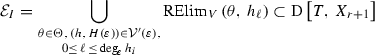
$$\begin{aligned} \mathbf {\Theta }=\bigcup _{\tau \in \mathcal {L}} \mathbf {\Theta }_\tau \subset \mathrm{D}\left[ T,\,X_{r+1},\,V\right] . \end{aligned}$$

Compute

$$\begin{aligned} \mathcal {E}=\mathcal {C} \cup \bigcup _{\theta \in \mathbf {\Theta }} \mathrm{RElim}_V(\theta ,\,\mathrm{Der}(\theta ))\subset \mathrm{D}\left[ T,\,X_{r+1}\right] , \end{aligned}$$

using [2], Algorithm 11.19 (Restricted Elimination)], so that the Thom encodings of the real roots of $\theta (t,\,x_{r+1},\,V)$ are fixed when $x_{r+1}$ varies in an open interval defined by the roots of the polynomials $\mathcal {E}(t).$

Step 3(e). :

Compute using [2], Algorithm 12.19 (Triangular Sign Determination)] the Thom encodings of the real roots of the polynomials in $\mathcal {E}(t)$ and the ordered list $c_1<\cdots < c_{h-1}$ of the roots of the polynomials in $\mathcal {E}(t)$ in the interval $(c_0,\,c_h),$ with $c_0=\alpha _1,\,c_h=\alpha _2.$ Denote by $C_j,\,\rho _j$ a polynomial in $\mathcal {E}(t)$ and a Thom encoding representing $c_j.$

Step 3(f). :

For every j from 1 to $h-1,$ and for every $\theta \in \mathbf {\Theta },$ determine, using [2], Algorithm 12.19 (Triangular Sign Determination)], the Thom encoding

$$\begin{aligned} \theta \left( t,\,c_j,\,V\right) ,\,\tau _j \end{aligned}$$

of a root $v_j$ such that $v_j=\lim _\varepsilon (v(\varepsilon )),$ where $v(\varepsilon )$ is the root of $\theta (\varepsilon )(t,\,c_j,\,V)$, with Thom encoding $\tau (\varepsilon ).$ The multiplicity $\mu _j$ of the root $v_j$ is determined by $\tau _j.$

Step 3(g). :

For every j from 1 to h, define $I=(c_{j-1},\,c_j).$ For every $\theta \in \mathbf {\Theta }$ determine, using [2], Algorithm 12.19 (Triangular Sign Determination)], the Thom encoding $\theta _{I}(t,\,x_{r+1},\,V),\,\tau _{I}$ of a root $v_{I}(x_{r+1})$ of multiplicity $\mu _I$ such that for every $x_{r+1}\in I,\,v_{I}(x_{r+1})=\lim _\varepsilon (v(\varepsilon ))$, where $v(\varepsilon )$ is the root of $\theta (\varepsilon )(t,\,x_{r+1},\,V)$ with Thom encoding $\tau (\varepsilon ).$ The multiplicity $\mu _I$ of the root $v_{I}(x_{r+1})$ is determined by $\tau _{I}.$

Step 3(h). :

Given $(\theta (\varepsilon ),\,\Theta (\varepsilon ))$ in $\mathcal {U}(\varepsilon )$, denote by $(g_{\Theta (\varepsilon )},\,G_{\Theta (\varepsilon )})$ the $k-r+1$-tuple of polynomials obtained by substituting into $(g(\varepsilon ),\,G(\varepsilon ))$ the variables $X^{\prime },\,U$ by $F(\varepsilon )$ (Notation 4.5). Denote by $\mathcal {V}^{\prime }(\varepsilon )\subset \mathrm{D}[\varepsilon ,\,T,\,X_j,\,V]$ the set of $k-r+1$-tuples of polynomials $(g_{\Theta (\varepsilon )},\,G_{\Theta (\varepsilon )}).$

Step 3(i). :

For every j from 1 to $h-1$ and every $(h(\varepsilon ),\,H(\varepsilon ))\in \mathcal {V}^{\prime }(\varepsilon ),$ with $H(\varepsilon )=(h(\varepsilon )_{0},\,h(\varepsilon )_{r+2},\ldots , h(\varepsilon )_{k})$, determine the order in $\varepsilon$ of

$$\begin{aligned} h_{\varepsilon }(t,\,c_j,\,v_j),\,h(\varepsilon )_{i}(t,\,c_j,\,v_j). \end{aligned}$$

This is done by determining the signs of the coefficient $h_{\ell },\,h_{i,\ell }$ of $\varepsilon ^\ell$ in $h(t,\,c_j,\,v_j),\,h_i(t,\,c_j,\,v_j)$ using [2], Algorithm 12.19 (Triangular Sign Determination)]. Retain those $(h(\varepsilon ),\,H(\varepsilon ))$ such that $o(h(\varepsilon )_{0})\le o(h(\varepsilon )_{i})$ for all i from $r+2$ to k, and replace $\varepsilon$ with $0$ in

$$\begin{aligned} (\varepsilon ^{-o(h_{\varepsilon })}h(\varepsilon ),\,\varepsilon ^{-o(h(\varepsilon )_{0})}H(\varepsilon )), \end{aligned}$$

which defines a set $\mathcal {H}_j.$ Inspecting every $(h,\,H)\in \mathcal {H}_j,$ determine, using [2], Algorithm 12.19 (Triangular Sign Determination)], a $k-r+1$-tuple $(h_j,\,H_j)$ with the following property. Let $d_j$ be the point represented by the real univariate representation

$$\begin{aligned} \left( h_j\left( T,\,X_{r+1},\,V\right) ,\,\tau _j,\,H_j^{(\mu _j-1)}\left( T,\,X_{r+1},\,V\right) \right) \end{aligned}$$

over $t,\,u.$ The image under $\lim _\varepsilon$ of the point of $S(\varepsilon )$ with the $X_{r+1}$-coordinate $(c_j)$ is $(z,\,c_j,\,d_j).$

Step 3(j). :

For every j from 1 to h, define $I=(c_{j-1},\,c_j).$ For every $(h(\varepsilon ),\,H(\varepsilon ))\in \mathcal {V}^{\prime }(\varepsilon ),$ with $H(\varepsilon )=(h(\varepsilon )_{0},\,h(\varepsilon )_{r+2},\ldots , h(\varepsilon )_{k})$, subdivide I so that the order in $\varepsilon$ of $h(\varepsilon )(t,\,c_j,\,v_j)$ and $h_i(\varepsilon )(t,\,x_{r+1},\,v_{I}(x_{r+1}))$ is fixed. This is done by computing

and

using [2], Algorithm 11.19 (Restricted Elimination)]. Defining

$$\begin{aligned} \mathcal {E}^{\prime }_I=\mathcal {E}_I\cup \bigcup _{i\in {0,r+2,\ldots ,k}} \mathcal {E}_{I,i}, \end{aligned}$$

compute the Thom encodings of the roots of the polynomials in $\mathcal {E}^{\prime }_{I}(t)$ using [2], Algorithm 12.19 (Triangular Sign Determination)]. On each open interval J between two successive roots, the order in $\varepsilon ,$ denoted by $o(h_{\varepsilon }),\,o(h(\varepsilon )_{i})$ of the polynomials

$$\begin{aligned} h(\varepsilon )\left( t,\,x_{r+1},\,v_{J}\left( x_{r+1}\right) \right) ,\,h_i(\varepsilon )\left( t,\,x_{r+1},\,v_{J}\left( x_{r+1}\right) \right) , \end{aligned}$$

remains fixed. Retain those $(h(\varepsilon ),\,H(\varepsilon ))$ such that $o(h(\varepsilon )_{0})\le o(h(\varepsilon )_{i})$ for all i from $r+2$ to k, and replace $\varepsilon$ with $0$ in $\varepsilon ^{-o(h(\varepsilon )_{0})}(h,\,H(\varepsilon )),$ which defines a set $\mathcal {H}_J.$ Inspecting every $(h,\,H)\in \mathcal {H}_J,$ determine, using [2], Algorithm 12.19 (Triangular Sign Determination)], a $k-r+1$-tuple $(h_J,\,H_J)$ such that the point represented by

$$\begin{aligned} \left( h_J\left( t,\,x_{r+1},\,v_{I}\right) ,\,H_J^{(\mu _J-1)}\left( t,\,x_{r+1},\,v_{I}\right) \right) \end{aligned}$$

is the image under $\lim _\varepsilon$ of the point of $S(\varepsilon )$ with the $X_{r+1}$-coordinate $x_{r+1},$ where $\mu _J$ is the multiplicity of $u_{J}(x_{r+1})$ as a root of $h_{J}(x_{r+1},\,V).$ Let $w_J$ be the curve represented by the curve segment representation

$$\begin{aligned} h_{I}\left( T,\,X_{r+1},\,U\right) ,\,\tau _j,\,H_J^{(\mu _J-1)}\left( T,\,X_{r+1},\,U\right) , \end{aligned}$$

with parameter $X_{r+1}$ over $t,\,u.$

Step 3(k). :

Let $c_1< \cdots < c_{N-1}$ denote the set of all elements of $\mathrm {R}$ computed earlier in Steps 2(d) and (i), and $c_N=c.$ Reindex each $v_j$ computed in Step 3(h) such that $d_j$ lies above $c_j.$ Similarly, reindex each $w_I$ computed in Step 3(i) by some $j,\,1 \le j \le N,$ so that $w_j$ lies above the interval $(c_{j-1},\,c_j).$ Output the lists consisting of $d_1,\ldots ,d_{N-1}$ and $w_1,\ldots ,w_N.$

Proof of correctness. Let $\gamma (\varepsilon ):\,(\alpha (\varepsilon )_{1},\,\alpha (\varepsilon )_{2}) \rightarrow \mathrm {R}\langle \varepsilon \rangle ^k$ be the curve represented by a well-parametrized curve segment

$$\begin{aligned} f(\varepsilon )_{1},\,\sigma (\varepsilon )_{1},\,f(\varepsilon )_{2},\,\sigma (\varepsilon )_{2},\,g(\varepsilon ),\,\tau (\varepsilon ),\,G(\varepsilon ) \end{aligned}$$

computed in Step 2.

Let $G:\,(\alpha _1,\,\alpha _2) \rightarrow \mathrm {R}^k$ be a curve whose image equals the image of $\gamma (\varepsilon )$ under $\lim _\varepsilon .$ Since the input curve segment is well parametrized, it follows from Proposition 8.7 that in order to compute for any $x_1 \in (c_0,\,c_N),\,G(x_1)$, it suffices to compute $\lim _\varepsilon \gamma (\varepsilon )(x_1).$ The proof of correctness of the algorithm is then similar to the proof of correctness of Algorithm 3 (Limit of a Bounded Point). $\square$

Complexity analysis. Let $\mathrm{D}$ be a bound on the degrees of all polynomials appearing in the input. We first bound the degrees in the various variables, $\varepsilon ,\,T,\,X^{\prime },\,X_{r+1},\,U,\,V$, of the polynomials computed in various steps of the algorithm. In Step 1, the degrees of the polynomials in $\mathcal {U}(\varepsilon )$ are bounded as follows. The degrees in $\varepsilon ,\,U$ are bounded by $D^{O(r)}$ by the complexity analysis of [2], Algorithm 12.18 (Parametrized Bounded Algebraic Sampling)], and the degrees in the $T_i$ are bounded by $\mathrm{D}$ because of the pseudoreduction. Moreover, the complexity of this step is bounded by $\mathrm{D}^{O(m+r)}$ from the complexity of [2], Algorithm 12.18 (Parametrized Bounded Algebraic Sampling)] and the complexity of pseudoreduction (Definition 4.2).

The degrees in $\varepsilon ,\,T_i,\,X^{\prime },\,U$ in the output of Step 2 are all bounded by $D^{O(1)}$, and the complexity of Step 2 is bounded by

$$\begin{aligned} (k-r)^{O(1)} \mathrm{D}^{O(m+r)} = k^{O(1)}\mathrm{D}^{O(m+r)} \end{aligned}$$

using the complexity analysis of Algorithm 8 (Reparametrization of a Curve).

The degrees of the polynomials in Step 3(a) are bounded as follows. In the output of the call to [2], Algorithm 12.18 (Parametrized Bounded Algebraic Sampling)], the degrees in $\varepsilon ,\,U$ are bounded by $\mathrm{D}^{O(r)},$ and the degrees in the $T_i$ are bounded by $\mathrm{D}.$ Now, from the complexity analysis of Algorithm 3 (Limit of a Bounded Point) it follows that the degrees in the $T_i$ of the polynomials output are bounded by $\mathrm{D}$, and those in $\varepsilon ,\,U$ are bounded by $\mathrm{D}^{O(r)}.$ Moreover, the complexity of Step 3(a) is bounded by $D^{O(m+r)}$ from the complexity of [2], Algorithm 12.18 (Parametrized Bounded Algebraic Sampling)], the complexity of Algorithm 3 (Limit of a Bounded Point), and the complexity of the pseudoreduction (Proposition 8.4).

The degrees of the polynomials in Step 3(b) are bounded as follows. In the output of the call to [2], Algorithm 12.18 (Parametrized Bounded Algebraic Sampling)], the degrees in $\varepsilon ,\,X_{r+1},\,V$ are bounded by $D^{O(r)},$ and the degrees in the $T_i$ are bounded by $\mathrm{D}.$ The complexity of Step 3(b) is bounded by $D^{O(m+r)}$ from the complexity of [2], Algorithm 12.18 (Parametrized Bounded Algebraic Sampling)] and the complexity of pseudoreduction (Definition 4.2).

The complexity of Step 3(c) is bounded by $D^{O(m+r)}$ using the degree bounds from the complexity analysis of the previous steps and the complexity of [2], Algorithm 12.23 (Triangular Sample Points)].

It now follows from the complexity analysis of [2], Algorithm 12.19 (Triangular Sign Determination)], [2], Algorithm 11.19 (Restricted Elimination)], and the degree estimates proved previously that the complexity of the remaining steps are all bounded by $k^{O(1)} \mathrm{D}^{O(m+r)}.$ Thus, the complexity of the algorithm is bounded by $k^{O(1)} \mathrm{D}^{O(m+r)}.$

References

S. Basu, R. Pollack and M.-F. Roy: Computing roadmaps of semi-algebraic sets on a variety. J. Amer. Math. Soc. 13(1), pages 55–82, 2000.
S. Basu, R. Pollack and M.-F. Roy: Algorithms in Real Algebraic Geometry, volume 10 of Algorithms and Computation in Mathematics, Second edition, Springer, Berlin, 2006.
S. Basu, R. Pollack and M.-F. Roy: Algorithms in Real Algebraic Geometry, volume 10 of Algorithms and Computation in Mathematics. Springer, Berlin, 2011, online version posted on 3 August 2011, available at http://perso.univ-rennes1.fr/marie-francoise.roy/.
J. Bochnak, M. Coste and M.-F. Roy: Géométrie algébrique réelle, Second edition in English: Real Algebraic Geometry), volume 12(36) of Ergebnisse der Mathematik und ihrer Grenzge- biete [Results in Mathematics and Related Areas], Springer, Berlin, 1987 (1998).
J. Canny: The Complexity of Robot Motion Planning, MIT Press, Cambridge, 1987.
G. E. Collins: Quantifier elimination for real closed fields by cylindric algebraic decomposition, Second GI Conference on Automata Theory and Formal Languages, volume 33 of Lecture Notes in Computer Science, pages 134–183, Springer, Berlin, 1975.
M. Coste, H. Lombardi and M.-F. Roy: Dynamical method in algebra: effective Nullstellensätze, Ann. Pure Appl. Logic, 111(3), pages 203–256, 2001.
M. S. el Din and E. Schost: A baby steps/giant steps probabilistic algorithm for computing roadmaps in smooth bounded real hypersurface, Discret. Comput. Geom. 45(1), pages 181–220, 2011.
L. Gournay and J. J. Risler: Construction of roadmaps of semi-algebraic sets, Appl. Algebra Eng. Commun. Comput. 4(4), pages 239–252, 1993.
D. Grigoriev and N. Vorobjov: Counting connected components of a semi-algebraic set in subexponential time, Comput. Complex. 2(2), pages 133–186, 1992.
D. Yu. Grigoriev, J. Heintz, M.-F. Roy, P. Solernó and N. N. Vorobjov Jr.: Comptage des composantes connexes d’un ensemble semi-algébrique en temps simplement exponentiel, C. R. Acad. Sci. Paris I 311(13), pages 879–882, 1990.
J. Heintz, M.-F. Roy, and P. Solernò. Single exponential path finding in semi-algebraic sets ii: The general case. In Chandrajit L. Bajaj, editor, Algebraic geometry and its applications, pages 449–465. Springer-Verlag, 1994. Shreeram S. Abhyankar’s 60th birthday conference, 1990.
J. Heintz, M.-F. Roy and P. Solernó: Single exponential path finding in semialgebraic sets. I. The case of a regular bounded hypersurface. In Applied Algebra, Algebraic Algorithms and Error-Correcting Codes (Tokyo, 1990), volume 508 of Lecture Notes in Computer Sciences, Springer, Berlin, 1991, pages 180–196.
J. Schwartz and M. Sharir: On the piano movers’ problem. II. General techniques for computing topological properties of real algebraic manifolds, Adv. Appl. Math. 4, pages 298–351, 1983.
N. N. Vorobjov Jr. and D. Yu. Grigoriev: Determination of the number of connected components of a semi-algebraic set in subexponential time, Dokl. Akad. Nauk SSSR 314(5), pages 1040–1043, 1990.
Acknowledgments
We are very grateful to the anonymous referees of the paper for their numerous suggestions. We are particularly grateful to one of them for pointing out an error in a preliminary version. The first author was supported in part by National Science Foundation Grants CCF-0915954, CCF-1319080, and DMS-1161629. The first and second authors did part of the work during a research stay in Oberwolfach as part of the Research in Pairs Programme. The third author is a member of Institut Universitaire de France and supported by a French National Research Agency EXACTA grant (ANR-09-BLAN-0371-01) and a GeoLMI grant (ANR-2011-BS03-011-06). The fourth author was supported by an NSERC Discovery Grant and by the Canada Research Chairs Program.
Author information
Authors and Affiliations
Corresponding author
Additional information
Communicated by Teresa Krick.