
Abstract
The paper adopts a single-country regional panel dataset to analyse the long-term relationship between agricultural greenhouse gases (GHG) emissions and productivity growth and, consequently, to assess emissions sustainability. The hypothesis of emission sustainability is assessed by estimating alternative panel model specifications with conventional and GMM estimators applied to the highly heterogeneous Italian regional agriculture, whose methane and nitrous oxide emissions are properly reconstructed for the periods 1951–2008 and 1980–2008. The modelling approach and the empirical specification include the environmental Kuznets curve (EKC) as one of the possible outcomes. Results suggest that, when a significant relationship between agricultural GHG emissions and productivity growth occurs, it is often monotonic and, though sustainability is accepted for some GHG, no univocal robust evidence of the EKC emerges across the different specifications, estimators and periods. Policy implications of this empirical evidence are finally drawn.


Notes
Compared to other studies, these estimates are even optimistic. For example, using different methodologies, the Worldwatch Institute (Goodland and Anhang 2009) estimates that the contribution of agriculture to GHG global emissions may currently exceed 50 %. FAO (2006) states that the livestock sector alone is responsible for 18 % of all GHG production.
Though it might be insufficient to achieve the global emission targets established at the international level where, in fact, a substantial reduction of GHG emissions is required over the next decades (OECD 2008), this definition of sustainability remains an interesting benchmark especially if this condition is met, on a global scale, with a growing level of agricultural production.
The IPCC actually includes six sources but one of them, source 4E-Prescribed burning of Savannas, is not relevant in Italy, therefore it will not be considered here.
This is the case of the Implied Emission Factor, IEF; see Sect. 4 for clarifications.
The relevance of the intra-sectoral composition effect is emphasised in a recent study for the EU Commission on climate change mitigation options focusing on the food sector (Faber et al. 2012). The difference in emission per unit of agricultural product is used to identify changes in dietary choices that could contribute to reduce emissions from agriculture and food production.
This different behaviour of \(VA_{t}/L_{t}\) and TFP over time is reflected in their respective stochastic properties. As will be shown in Sect. 7.1, while \(VA_{t}/L_{t}\) is stationary within the panel, the agricultural TFP shows a unit root.
Assuming stationarity around the mean of \(g_{Lt}\) and \(g_{Pt}\) does not imply stationarity around the mean of \(p_{t}\) and \(\ln L_{t}\). However, if \(p_{t}\) and \(\ln L_{t}\) are stationary around a deterministic trend or are I(1) processes, it follows that \(g_{Lt}\) and \(g_{Pt}\) are stationary around the mean. These stochastic properties will be confirmed, for the case under analysis, in Sects. 5.3 and 7.1.
In the specific case under investigation here (Italian regions over period 1951–2008 or 1980–2008), the assumptions \(g_{Pt} >0\) and \(g_{Lt} <0\) are fully consistent with observed data (see Sect. 5).
Conditions \(h\le \frac{\lambda }{\gamma }- 1\) and \(h\le \frac{\lambda }{\gamma }\) can be empirically assessed by taking the average \(\lambda \) and \(\gamma \) observed within the sample under investigation (see next sections).
In the present application \(\hbox {N}=20\) and \(\hbox {T}= 29\) and 58 for the short and long time series, respectively (see below).
In performing model estimation, the one-lag specification has been chosen among alternative AR(p) specifications according to the AIC (Akaike Information Criterion).
For the sake of simplicity, in the case of \(\hbox {CH}_{4}\), “short series” here identifies the 1980–2008 period, “long series” the 1951–2008 period (see Sect. 5 for details). By aggregating the emission series of \(\hbox {CH}_{4}\) and \(\hbox {N}_{2}\hbox {O}\) on the basis of their Global Warming Potential (GWP), it is also possible to reconstruct the whole agricultural GHG emission expressed in terms \(\hbox {CO}_{2}\)eq. for the period 1980–2008. All the analysis and estimates here proposed have been also performed for this aggregate \(\hbox {CO}_{2}\)eq. series. As they simply combine what separately obtained for \(\hbox {CH}_{4}\) and \(\hbox {N}_{2}\hbox {O}\), these results are not reported here but available upon request.
This range of variation of the Italian regional sample is delimited by the lower bounds Umbria-1951 (for \(p_t\)) and Liguria-2008 (for \(e_{kit}^{V}\)) and the upper bounds Toscana-2008 (for \(p_{t}\)) and Valle d’Aosta-1951 (for \(e_{kit}^{V}\)). The same behaviour of \(e_{kit}^{V}\) can be observed for \(e_{kit}^{L}\); for space limitation this latter case is not reported here but can be obtained upon request.
Fig. 2 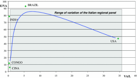
Range of variation of yearly E/VA (g per 1995 US $) and VA/L (thousand 1995 US $ per labour unit) in the Italian regional panel 1951–2008 (grey area) and in selected countries in the last decade (2000–2005). Source: Elaborations on FAO, IPCC and Agrefit (Rizzi and Pierani 2006) data
For \({VA_t}/{L_t}\), country data are taken from FAO and are expressed in 1995 US $ per unit of agricultural population. To make data comparable in Fig. 2, also Italian regional data for \(VA_{t}\) have been expressed in 1995 US $. Data on country–level \(E_{t}\) come from UNFCCC submissions. While agricultural emission data are regularly collected and released for Appendix countries (Kyoto Protocol) following the IPCC guidelines, for non-Appendix countries (therefore, less developed, developing and emerging countries) comparable emission data are infrequent. However, some of these updated and comparable data are provided by the voluntary national communications to the UNFCCC. Besides USA (2005), these data concern China (2005), Brazil, India and Congo (2000). Therefore, these are the countries here considered.
Although field burning of crop residues (4F) is forbidden in Europe, Italy is one of few countries that still reports figures from this minor source category.
\(\hbox {CO}_{2 }\)and fluorine gas emissions from these sources are negligible and \(\hbox {CO}_{2}\) emissions and removals from land use, land-use change and forestry, are reported under another Category (LULUCF) and estimated with a different methodology.
More details on this top–down methodology can be found in De Lauretis et al. (2009).
Agrefit database is freely available at www.agriregionieuropa.it.
In Italy, area cultivated adopting single aeration is a very little share of the total rice area, and this practice has been mainly used since 1990.
It is worth noticing that the IEFs used in both the top–down and the bottom–up reconstruction are not available at regional level. The national IEFs are applied to the respective regional activity data to obtain all regional emission series. It follows that it is not possible to distinguish at the regional level the variation of GHG emissions coming from intra-sectoral composition and that generated by technological change, this latter being mostly expressed by a variation of the IEF associated to a given activity.
VA is expressed in million € at 1995 constant prices, while \(L\) is expressed in thousand units.
It is also worth reminding that the adopted panel test (CIPS) is not simply the combination of individual ADF tests as it includes the cross-sectional dependence (therefore, the individual CADF tests) (Pesaran 2007).
Due to space limitations, these regional test results cannot be reported here for all variables. They are available upon request.
The Augmented Dickey-Fuller (ADF)-GLS test is a modified ADF test with significantly greater power than the conventional ADF test, especially under near unit-root processes and small sample size. Unlike the ADF test, in the Kwiatkowski-Phillips-Schmidt-Shin (KPSS) test the null hypothesis is that the series is I(0), while in the alternative hypothesis, is I(1). Therefore, the KPSS test is expected to reveal those series that the conventional ADF test tends to accept as I(1) while, in fact, they are only near unit-root processes.
GMM estimation has been obtained using all admitted lags as instruments. To maintain consistency and robustness of the estimated standard errors, only the one-step GMM estimation is here performed (Arellano 2003).
In all GMM estimations the Hansen–Sargan test confirms that the selection of instruments is appropriate, while the Arellano-Bond autocorrelation test accepts the adopted dynamic specification as first order correlation is observed but no second order correlation. The results of all these tests are available upon request. In the case of \(\hbox {CH}_{4}\) (long series), for instance, test results are the following (\(p\) value in parenthesis). For specification (5a), the Sargan test is 892.12 (0.79), the Arellano-Bond test is -2.25 (0.02) for the first order autorcorrelation and 1.36 (0.17) for the second order autorcorrelation. For specification (5b), the Sargan test is 827.25 (0.98), the Arellano-Bond test is \(-\)1.696 (0.09) for the first order autorcorrelation and 1.026 (0.30) for the second order autorcorrelation.

References
Arellano M (2003) Panel-data econometrics. Oxford University Press, Oxford
Baldock D, Bartley J, Framer M, Hart K, Lucchesi V, Silcock P, Zobbe H, Pointereau P (2007) Evaluation of the environmental impacts of CAP (Common Agricultural Policy) measures related to the beef and veal sector and the milk sector. Alliance Environ
Baltagi BH (2005) Econometric analysis of panel data. Wiley, New York
Beck N (2001) Time-series-cross-section data: what have we learned in the past few years. Annu Rev Political Sci 4:271–293
Bellarby J, Tirado R, Leip A, Weiss F, Leeschen JP, Smith P (2013) Livestock greenhouse gas emissions and mitigation potential in Europe. Glob Change Biol 19(1):3–18
Borghesi S, Vercelli A (2009) Greenhouse gas emissions and the energy system: are current trends sustainable? Int J Glob Energy Issues 32:160–174
Brock WA, Taylor MS (2005) Economic growth and the environment: a review of theory and empirics. In: Aghion P, Durlauf S (eds) Handbook of economic growth, Ch. 28, vol 1. Elsevier, Amsterdam, pp 1749–1821
Chimeli AB, Braden JB (2005) Total factor productivity and the environmental Kuznets curve. J Environ Econ Manag 49:366–380
Coderoni S (2010) I principali effetti della Politica Agricola Comune sui dati di attività utilizzati per stimare le emissioni di gas serra del settore agricolo italiano dal 1990 al 2007. Institute for Environmental Protection and Research—ISPRA, Internship Thesis, Rome
Coderoni S, Esposti R (2013) Emissioni di metano e crescita della produttività nell’agricoltura italiana. Tendenze di lungo periodo e scenari futuri. Questione Agraria—Rivista dell’Associazione Rossi-Doria, n. 3/2013 (in press)
Costantini V, Martini C (2010) A modified environmental Kuznets curve for sustainable development assessment using panel data. Int J Glob Environ Issues 10(1–2):84–122
De cara S, Houzé M, Jayet P-A (2005) Methane and nitrous oxide emissions from agriculture in the EU: a spatial assessment of sources and abatement costs. Environ Resour Econ 32:551–583
De Lauretis R, Caputo A, Cóndor R D, Di Cristofaro E, Gagna A, Gonella B, Lena F, Liburdi R, Romano D, Taurino E, Vitullo M (2009) La disaggregazione a livello provinciale dell’inventario nazionale delle emissioni. Institute for Environmental Protection and Research—ISPRA, Technical report 92/2009, Rome
Dick J, Smith P, Smith R, Lilly A, Moxey A, Booth J, Campbell C, Coulter D (2008) Calculating farm scale greenhouse gas emissions. University of Aberdeen, Carbon Plan, the Macaulay Institute, Pareto consulting, SAOS Ltd, Scotland
Elliott G, Rothenberg TJ, Stock JH (1996) Efficient tests for an autoregressive unit root. Econometrica 64:813–836
EMEP/EEA (2009) Air pollutant emission inventory guidebook 2009. Technical guidance to prepare national emission inventories, Technical report No 9/2009, EEA- European Environment Agency, Copenhagen (http://www.eea.europa.eu/publications/emep-eea-emission-inventory-guidebook-2009/#)
Enders W (1995) Applied econometric time series. Wiley, NY
Esposti R (2000) Stochastic technical change and procyclical TFP: the Italian agriculture case. J Prod Anal 14(2):117–139
Esposti R (2007a) Regional growth and policies in the European Union: does the common agricultural policy have a counter-treatment effect? Am J Agric Econ 89:116–134
Esposti R (2007b) On the decline of agriculture. Evidence from Italian Regions in the Post-WWII Period. Working Paper Series n. 300, Department of Economics and Social Sciences, Università Politecnica delle Marche, Ancona (Italy)
Esposti R (2010) On why and how agriculture declines. Evidence from Italian regions in the post-WWII period. In: Boccaletti S (ed) Cambiamenti nel sistema alimentare: nuovi problemi, strategie, politiche, Atti del XLVI Convegno SIDEA, 16–19 Settembre, Franco Angeli, pp 341–360
Esposti R (2011) Convergence and divergence in regional agricultural productivity growth. Evidence from Italian regions, 1951–2002. Agric Econ 42(2):153–169
Esposti R (2012) The driving forces of agricultural decline: a panel-data approach to the Italian regional growth. Can J Agric Econ 60(3):377–405
European Commission (2009) A reform agenda for a global Europe (reforming the budget, changing Europe), The 2008/2009 EU budget review. DRAFT 6-10-09, European Commission, Brussels
European Commission (2012) Proposal for a decision of the European parliament and of the council on accounting rules and action plans on greenhouse gas emissions and removals resulting from activities related to land use, land use change and forestry, COM(2012) 93 final, Brussels
European Environment Agency (2008) Report greenhouse gas emission trends and projections in Europe 2008. Tracking progress towards Kyoto targets, EEA-European Environment Agency, Copenhagen
European Environment Agency (2012) Annual European Union greenhouse gas inventory 1990–2010 and inventory report 2012 Submission to the UNFCCC Secretariat, ISSN 1725–2237 EEA-European Environment Agency, Copenhagen
Faber J, Sevenster M, Markowska A, Smit M, Zimmermann K, Soboh R, van ‘t Riet J (2012) Behavioural climate change mitigation options. Domain Report Food, CE Delft, Delft
FAO (2003) World agriculture: towards 2015/2030. An FAO perspective. FAO, Rome
FAO (2006) Livestock long shadow. Environmental issues and options. FAO, Rome
Galeotti M, Manera M, Lanza A (2009) On the robustness of robustness checks of the environmental Kuznets curve hypothesis. Environ Resour Econ 42:551–574
Garnett T (2011) Where are the best opportunities for reducing greenhouse gas emissions in the food system (including the food chain)? Food Policy 36(S1):S23–S32
Goodland R, Anhang A (2009) Livestock and Climate Change. What if the key actors in climate change are ...cows, pigs, and chickens? World Watch, November/December. World/Watch Institute, Washington, DC, USA, pp 10–19
Granger CWJ, Hallman JJ (1988) The algebra of I(1). Finance and economics discussion series. Board of Governors of the Federal Reserve System, Washington, DC
Holdren JP, Ehrlich PR (1974) Human population and the global environment. Am Sci 62:282–292
Hong SH, Wagner M (2008) Nonlinear cointegration analysis and the environmental Kuznets curve. Economics Series n. 224, Institute for Advanced Studies, Wien
Im KS, Pesaran MH, Shin Y (2003) Testing for unit roots in heterogeneous panels. J Econom 115:53–74
ISPRA (2010) Italian greenhouse gas inventory 1990–2008. National Inventory Report 2010. Institute for Environmental Protection and Research—ISPRA, Report 113/2010, Rome
Istat (1980–1984) Annuario di statistica agraria. Istat, Rome.
ISTAT (1985–1993) Statistiche dell’agricoltura, zootecnia e mezzi di produzione. ISTAT, Rome
ISTAT (1994–2008) Statistiche dell’agricoltura. ISTAT, Rome
Karlsson S, Lothgren M (2000) On the power and interpretation of panel unit root tests. Econ Lett 66(3):249–255
Kaya Y (1990) Impact of carbon dioxide emission control on GNP growth: interpretation of proposed scenarios. Paper presented to IPCC Energy and Indusry Sub-Group, Response Strategies Working Group, Paris
Khanna N, Plassmann F (2007) Total factor productivity and the environmental Kuznets curve: a comment and some intuition. Ecol Econ 63:54–58
Kijima M, Nishide K, Ohyama A (2010) Economic models for the environmental Kuznets curve: a survey. J Econ Dyn Control 34:1187–1201
Kiviet JF (1995) On bias. Inconsistency and efficiency of various estimators in dynamic panel data models. J Econom 68:53–78
Lewandowski P (2007) PESCADF: Stata module to perform Pesaran’s CADF panel unit root test in presence of cross section dependence. Statistical Software Component, No. S456732, Boston College Department of Economics
Liu G, Skjerpen T, Swensen A R, Telle R (2006) Unit roots, polynomial transformations and the environmental Kuznets curve. Discussion Papers No. 443, Statistics Norway, Research Department, Oslo
MacKinnon JG (1996) Numerical distribution functions for unit root and cointegration tests. J Appl Econom 11:601–618
Maddison D (2006) Environmental Kuznets curves: a spatial econometric approach. J Environ Econ Manag 51:218–230
Maddison D, Rehdanz K (2008) Carbon emissions and economic growth: homogeneous causality in heterogeneous panels. Kiel Working Papers1437, Kiel Institute for the World Economy
Mazzanti M, Montini A, Zoboli R (2008) Environmental Kuznets curve for air pollutant emissions in Italy: evidence from environmental accounts NAMEA panel data. Econ Syst Res 20(3):279–305
Metz B, Davidson OR, Bosch PR, Dave R, Meyer LA (eds) (2007) Climate change 2007: mitigation. Cambridge University Press, Contribution of Working Group III to the Fourth Assessment Report of the Intergovernmental Panel on Climate Change, Cambridge
OECD (2008) Environmental outlook to 2030. OECD, Paris
Pesaran MH (2007) A simple panel unit test in the presence of cross section dependence. J Appl Econom 22:265–312
Rizzi PL, Pierani P (2006) Agrefit. Ricavi, costi e produttività dei fattori nell’agricoltura delle regioni italiane 1951–2002. Associazione Alessandro Bartola, Franco Angeli Editore, Milan
Smith P, Fang C, Dawson JJC, Moncreiff JB (2008a) Impact of global warming on soil organic carbon. Adv Agron 97:1–43
Smith P, Martino D, Cai Z, Gwary D, Janzen H, Kumar P, McCarl B, Ogle S, O’Mara F, Rice C, Scholes B, Sirotenko O, Howden M, McAllister T, Pan G, Romanenkov V, Schneider U, Towprayoon S, Wattenbach M, Smith J (2008b) Greenhouse gas mitigation in agriculture. Philos Trans R Soc B 363:789–813
Stephenson J (2010) Livestock and climate policy: less meat or less carbon? Round table on sustainable development (SG/SD/RT(2010) 1). OECD, Paris
Stern DI (2004) The rise and fall of the environmental Kuznets curve. World Dev 32(8):1419–1439
Syrquin M (1988) Patterns of structural change. In: Chener H, Srinivasan TN (eds) Handbook of development economics, vol I. Elsevier, Amsterdam, pp 203–273
Timmer CP (1988) The agricultural transformation. In: Chener H, Srinivasan TN (eds) Handbook of development economics, vol I. Elsevier, Amsterdam, pp 275–331
Timmer CP (2002) Agriculture and economic development. In: Gardner B, Rausser G (eds) Handbook of agricultural economics, vol 2A. Elsevier, Amsterdam, pp 1487–1546
Author information
Authors and Affiliations
Corresponding author
Appendix
Appendix
See Tables 8, 9, 10, 11 and Fig. 2.
Rights and permissions
About this article
Cite this article
Coderoni, S., Esposti, R. Is There a Long-Term Relationship Between Agricultural GHG Emissions and Productivity Growth? A Dynamic Panel Data Approach. Environ Resource Econ 58, 273–302 (2014). https://doi.org/10.1007/s10640-013-9703-6
Accepted:
Published:
Issue Date:
DOI: https://doi.org/10.1007/s10640-013-9703-6