Learning from multiple annotators with varying expertise

Abstract

Learning from multiple annotators or knowledge sources has become an important problem in machine learning and data mining. This is in part due to the ease with which data can now be shared/collected among entities sharing a common goal, task, or data source; and additionally the need to aggregate and make inferences about the collected information. This paper focuses on the development of probabilistic approaches for statistical learning in this setting. It specially considers the case when annotators may be unreliable, but also when their expertise vary depending on the data they observe. That is, annotators may have better knowledge about different parts of the input space and therefore be inconsistently accurate across the task domain. The models developed address both the supervised and the semi-supervised settings and produce classification and annotator models that allow us to provide estimates of the true labels and annotator expertise when no ground-truth is available. In addition, we provide an analysis of the proposed models, tasks, and related practical problems under various scenarios. In particular, we address how to evaluate annotators and how to consider cases where some ground-truth may be available. We show experimentally that annotator expertise can indeed vary in real tasks and that the presented approaches provide clear advantages over previously introduced multi-annotator methods, which only consider input-independent annotator characteristics, and over alternative approaches that do not model multiple annotators.

1 Introduction

The ease with which data can be shared, organized, and processed by an increasingly larger number of entities is creating a number of interesting problems and opportunities for machine learning and data modeling in general. One of the main ramifications is that the knowledge from these different entities, in particular people, can now be easily collected and compounded in a distributed fashion. There are numerous examples of this effect, the classical instances being open source (e.g., Linux) and more recently Wikipedia, but this includes most forms of expert (and non-expert) group opinions or ratings, and on-line user behavior in general. However, combining or aggregating the knowledge from different sources is far from being a solved problem. In this paper, we concentrate on efficiently utilizing the type of knowledge provided by different human annotators, also referred to as labelers, sources, or experts. This setting also applies to other forms of data aggregation; for example, from different sensors or knowledge sources in general.

Supervised learning traditionally relies on a domain expert playing the role of a teacher providing the necessary supervision. The most common case is that of an expert providing annotations that serve as data point labels in classification problems. The above crowdsourcing effect (Howe 2008) motivates a natural shift from the traditional reliance on a single domain expert to several domain experts or even many more non-experts who contribute to a specific (learning) task. In supervised learning, more labeled data for training normally translates, under some assumptions and data size conditions, to higher test accuracy. What do more labelers/annotators translate to and how can their knowledge be efficiently utilized? Now the learning algorithm can have access to a labeler (pseudo) identity in addition to the usual label values. How can this information help? This paper tackles these problems in the context of learning from multiple annotators.

The availability of more annotators is not the only motivation for learning from multiple labelers. The multi-labeler setting is important to address real problems for which supervised learning is not suitable. In many application areas, there are problems for which obtaining the ground-truth labels is simply impossible or very costly. For example, in cancer detection from medical images (e.g., computer tomography, magnetic resonance imaging), an image region or volume associated to a body tissue can often be tested for the actual presence of cancer only by performing a biopsy; this is clearly a costly, risky procedure. In addition, many other annotation tasks are subjective by nature and thus there is no clear correct label. Almost any subjective opinion task falls in this category, from on-line product ratings to medical imaging diagnosis based on multi-expert opinions.

In multi-labeler problems, building a classifier in the traditional single expert manner, without regard for the label source (annotator) properties may not be effective in general. The reasons for this include: some annotators may be more reliable than others, some may be malicious, some may be correlated with others, there may exist different prior knowledge about annotators, and in particular annotator effectiveness may vary depending on the data instance presented. We believe this last element is of great importance and has not been clearly considered in previous approaches.

This paper also addresses a different facet of this problem. Even when multiple annotators are available, labels still have a cost. It is very generally the case that obtaining labels for data points can be expensive and time-consuming. We draw some parallel with semi-supervised learning and explore the question of how we can exploit data that has not been annotated by any labeler or that has only been annotated by some labelers. One natural approach would consist of ignoring any unlabeled data point. While this is valid and appropriate under some models, it is not very data efficient. As will be seen, our initial model (and all multi-labeler models proposed so far) would treat the unlabeled data in this manner. In this paper we propose a different strategy for this new problem based on using the properties of the unlabeled data distribution. This approach provides clear advantages when compared to multi-annotator methods that do not use the unlabeled data and over semi-supervised methods that do not use multi-labeler information.

Parts of this paper were published in Yan et al. (2010a, 2010b). This paper offers a more complete view of the problem and a unified treatment of two learning settings initially approached separately. The key differences are the inclusion of a more thorough literature review (Sect. 2), the addition of a few more details in the formulation and on the derivations of the parameter update equations utilized by the algorithms (Sects. 3 and 5). Most of the new work was directed towards an extended experimental evaluation for both the supervised and semi-supervised settings and the development of the proposed annotator evaluation strategy. Specifically, a new set of experiments related to the supervised setting with different amounts of ground-truth was conducted and is part of this paper (Sect. 7.2). This required a modification of the initially proposed learning algorithm. The proposed evaluation strategy (Sect. 4), was thoroughly developed and tested (Sect. 7.3). New data sets are included in the semi-supervised learning experiments (Sect. 7.4), in particular one with a large number of annotators (IMDB) and another data set designed/collected specifically for this paper (AF).

We believe this paper advances the field by bringing together a quite complete set of modeling tools, experiments, and insights to address the multi-labeler machine learning problem from a common probabilistic viewpoint. We have not seen this collection of topics addressed together and extensively tested in the variety of tasks presented in this paper.

2 Related work

The problem of modeling data that has been processed by multiple annotators has been receiving increasing attention. However, similar problems have been studied for quite some time. For example, in clinical statistics, Dawid and Skeene (1979) studied the problem of error rate estimation given repeated but conflicting responses (labels) of patients to various medical questions. In this work, a point estimate of individual error rates was identified using latent variable models. Later, Spiegelhalter and Stovin (1983) used this model to quantify residual uncertainty of the label value.

We can divide the related work in multi-labeler classification in various sub-areas. One area of work consists on the estimation of error rates for the labelers independently from building a classifier. Both early works above (Dawid and Skeene 1979; Spiegelhalter and Stovin 1983) and others such as Hui and Zhou (1998), fall in this area, while more recently Snow et al. (2008) showed that employing multiple non-expert annotators can be as effective as employing one expert annotator when building a classifier.

Very recently, the interest has shifted towards more directly building classifiers from multi-labeler data. In this area, we can subdivide the approaches into those attempting to use repeated labeling or prior knowledge about labeler similarities. Repeated labeling (Smyth et al. 1994; Donmez and Carbonell 2008; Sheng et al. 2008) relies on the identification of what labels should be reacquired in order to improve classification performance or data quality. This form of active learning can be well suited when we can control assignments of data points to labelers. However, Dekel and Shamir (2009) provided arguments indicating that this approach is wasteful and negatively impacts the relative size of the training set. Approaches based on prior knowledge rely on the existence of some way to measure labeler relationships. These include the work of Crammer et al. (2008), where labeler similarities and their labels are used to identify what samples should be used to estimate classification models for each labeler, and Blitzer et al. (2008) where the multiple labels are obtained by labeling data drawn from multiple underlying domains (in the context of domain adaptation).

Application areas for multi-labeler learning vary widely. These include natural language processing (Snow et al. 2008), computer-aided diagnosis/radiology (Raykar et al. 2009; Spiegelhalter and Stovin 1983), clinical data integration (Dawid and Skeene 1979), and computer vision (Sorokin and Forsyth 2008).

The base multi-labeler approach proposed in this paper differs from the related work in various axes. Unlike Dawid and Skeene (1979) and Spiegelhalter and Stovin (1983), we produce labeler error estimates and simultaneously build a classifier in a combined process. In contrast to Smyth et al. (1994) and Sheng et al. (2008), we do not assume that labels can be reacquired and thus a different setting is addressed. Also, we do not assume the existence of any prior information relating the different labelers or the domains from where the data is drawn, such as Crammer et al. (2008) or Blitzer et al. (2008).

The supervised multi-labeler setting addressed in this paper is more related to that provided in Raykar et al. (2009), Jin and Ghahramani (2003), and Welinder et al. (2011), but the approach differs as follows. Like the approaches presented by Raykar et al. (2009) and Welinder et al. (2011) and to some extent that by Jin and Ghahramani (2003), this paper estimates the error rates and the classifier simultaneously; however, unlike these approaches this paper models the error rates of the labelers as dependent on the data points.

An interesting derived problem we study in this paper is the automatic determination of annotator reliability or adversarial nature. The approach proposed by Raykar and Yu (2011) has a similar goal. However, the proposed spammer score is based on the annotator specificity and sensitivity (which is constant across the data). The approach presented in this paper is different in two ways: (1) the annotator reliability is a function of the input observed and (2) it is defined using a different motivation, in terms of how surprising the labels provided by the annotator are conditioned on labels by other annotators and the learned model.

Outside of the area of supervised learning, multi-labeler learning is also related to problems of knowledge corroboration (Kasneci et al. 2011) and annotator selection. The latter includes repeated labeling (Smyth et al. 1994; Donmez and Carbonell 2008; Sheng et al. 2008), the process of identifying labels that should be revised in order to improve classification performance, and more recently (Paquet et al. 2010), a manner of learning where annotators are chosen randomly and then their responses corroborated using a separate model.

In the semi-supervised learning domain, with the exception of our recent work (Yan et al. 2010b), we are not aware of previous approaches for solving multi-labeler classification problem in this scenario (that is, combining multiply-labeled data with unlabeled data). However, in recent years many semi-supervised learning methods for classification have been introduced (see Zhu 2006 for a survey). Two main scenarios have been commonly considered when training a semi-supervised model: the transductive and inductive scenarios. In the transductive setting, the learner needs to observe the unlabeled testing data while training; and therefore, although accurate, these transductive models need to be retrained (or updated) every time a test sample is to be classified. As a result, transductive algorithms may not satisfy the run-time requirements for many real-world applications, including medical diagnosis applications where new patient cases need to be classified in real-time as part of the physician’s workflow. In the inductive setting, testing data is not assumed to be present at the time of model training. The semi-supervised, multi-labeler approach proposed in this paper is in the inductive category.

Most state-of-the art approaches for semi-supervised learning are based on a weighted graph (e.g., the graph Laplacian) (Belkin et al. 2004; Blum and Chawla 2001; Corduneanu and Jaakkola 2005; Krishnapuram et al. 2005; Zhou et al. 2004) where labeled and unlabeled points constitute the vertices of a graph and the similarities between the data point pairs are represented by its edge weights. Given this graph that contains information about the spatial proximity of the training data (labeled and unlabeled), the main idea behind these methods is the notion that the classification function to be learned should give similar values for neighboring points. In other words, the value of the separator function should change smoothly over neighboring data points. Our approach borrows from this fundamental idea from the semi-supervised scenario and studies whether it can be useful in the multiple annotator setting. Various possibilities are considered in this paper.

A distinguishing factor throughout this paper is that, unlike any approaches above, it is not assumed that expert reliability or error rate is consistent across all the input data even for one task. This is a flawed assumption in many cases since annotator knowledge can fluctuate considerably depending on the input instance. In this paper, the classifiers are built so that they take into account that some labelers are better at labeling some types of points (compared with other data points).

3 A general approach for modeling annotator expertise

Throughout this paper we consider a set of N data points X={x ₁,…,x _N } drawn independently from an input distribution and each labeled by at most T labelers/annotators. Let us denote $Y=\{y_{i}^{(t)}\}_{it}$ with $y_{i}^{(t)}$ the label for the i-th data point given by annotator t. In the setting addressed in this paper the labels from individual labelers might be incorrect, missing, or inconsistent with respect to each other. We introduce additional variables Z={z ₁,…,z _N } to represent the true but usually unknown label for the corresponding data point.

We let x _i and z _i for i∈{1,…,N} be random variables in the input space ${{{\mathcal{X}}}}$ and output space ${{{\mathcal{Z}}}}$ respectively. Similarly, we let $y_{i}^{(t)}$ be random variables over the space of labels ${{{\mathcal{Y}}}}$, where t∈{1,…,T}. If we do not have access to the ground-truth (or this does not exist), all of the variables z _i are unobserved. We concentrate on this more general case; however, in some problem instances partial ground-truth may be available. Some labels $y_{i}^{(t)}$ might be unknown as well, depending on the problem setting presented.

Given training data, X and Y, our goals are to produce: an estimate for the ground-truth Z=[z ₁,…,z _N ]′, a classifier for predicting the label z for new instances x, and a model of the annotators’ expertise as a function of the input x.

3.1 Base probabilistic model

Various elements need to be considered to appropriately model data that has been annotated by multiple sources. The key considerations are how to model annotator-specific characteristics, what should these depend on, and what influence these have in the labels they provide.

In modeling multiple annotators, we consider the annotation provided by labeler t to depend on the true (but usually unknown) label z and the input data point x. Our motivation for this is that annotators may label certain data points with better accuracy than other data points and that this accuracy may depend on the properties of the data point itself. That is, their accuracy depend on the input being presented. In addition, labelers are assumed independent given the input data point and the true point label.

In other words, we do not assume that annotators are equally good (or bad) at labeling all the data, but it depends on what input they observe.

These considerations have been made explicit in the probabilistic model over random variables x, y, and z with a graphical model as shown in Fig. 1. The joint conditional distribution can be expressed as:

$$\begin{aligned} p(Y,Z|X) =\prod_i p(z_i| \mathbf{x}_i) \prod_t p \bigl(y^{(t)}_i|\mathbf {x}_i, z_i \bigr). \end{aligned}$$

Fig. 1

Graphical model for x, y, and z respectively inputs, annotator-specific labels, and ground-truth label (for simplicity α,β,{γ _t }, and {w _t }, with t∈{1,…,T}, are excluded)

As can be seen from the model, we make the assumption that the labelers t={1,…,T} are independent given the input and the true label. In order to further specify our model we need to define the form of the conditional probabilities. In this paper, we explored several variations. Let us consider each conditional distribution in turn.

$p(y^{(t)}_{i}|\mathbf{x}_{i}, z_{i})$::

Our simplest model assumes that each annotator t provides a noisy version of the true label z:

$$\begin{aligned} p\bigl(y^{(t)}_i|\mathbf{x}_i, z_i\bigr) = p\bigl(y^{(t)}_i|z_i \bigr)={\bigl(1-\eta^{(t)}\bigr)}^{|y^{(t)}_i-z_i|}{\eta ^{(t)}}^{1-|y^{(t)}_i-z_i|} \end{aligned}$$

(1)

with $\mathcal{ Z} \equiv\mathcal{ Y}=\{0,1\}$. In this Bernoulli model, the parameter η ^(t) is the probability that labeler t is correct (i.e., y _i =z _i ). Another option we consider is the Gaussian model, where every labeler is expected to provide a distorted version of the true continuous output z:

$$\begin{aligned} p\bigl(y^{(t)}_i|z_i\bigr) = \mathcal{ N} \bigl(y^{(t)}_i;z_i,\sigma^{(t)}\bigr). \end{aligned}$$

(2)

This Gaussian distribution associates a lower variance σ ^(t) to more consistently correct labelers compared to inconsistent labelers. Note that we employ a distribution for continuous random variables, which is more natural for regression rather than classification models (for y continuous). In these models, where we assume that $p(y_{i}^{(t)}|\mathbf{x}_{i},z_{i})=p(y_{i}^{(t)}|z_{i})$, the additional independence assumptions mean that the graphical model is Markov-equivalent to the model x→z→{y ^(t)}. This is comparable to the models proposed by Raykar et al. (2009) and Jin and Ghahramani (2003), albeit with different parameterizations.

We use these models as a base for considering more general cases, where we will allow p(y|x,z)≠p(y|z). In our experience with real applications, we noticed that the quality of labels by annotators is not only a function of their expert level, but also of the type of data presented to them as well. For example, radiologists will have difficulty providing quality labels on blurry images. Additionally, some labelers will be more affected by blurry images than others and moreover some labelers are more knowledgeable for some input types than others. In general, annotators will exhibit varying levels of expertise in different types of data. We believe this is particularly true for non-expert annotators, albeit not necessary in all cases.¹

In order to model this input-dependent variability, we replace the previously described Gaussian model with the following:

$$\begin{aligned} p\bigl(y^{(t)}_i|\mathbf{x}_i,z_i \bigr) = & \mathcal{ N}\bigl(y^{(t)}_i;z_i, \sigma _{t}(\mathbf{x}_i)\bigr), \end{aligned}$$

(3)

where the variance now depends on the input x and is also specific to each annotator t.

The above conditional assumes y ^(t) is a continuous random variable. Thus, it is really suited for regression. In case we need to use this model for classification we would need to constrain σ _t (x). Since for classification y ^(t) can only take the binary values 0/1, we constrain σ _t (x) to be in the range between (0,1] by letting σ _t (x) be a logistic function of x _i and t:

$$\begin{aligned} \sigma_t(\mathbf{x}) = & \bigl(1+\exp\bigl(- \mathbf{w}_{t}^T \mathbf{x}_i - \gamma_t\bigr)\bigr)^{-1}, \end{aligned}$$

(4)

where a small constant can be added to σ _t (x) to prevent it to take the zero value in practice, particularly when data is scarce.

Similarly, we modify our Bernoulli model by setting η _t (x) to be also now a function of both x _i and t:

$$ p\bigl(y^{(t)}_i|\mathbf{x}_i,z_i \bigr) = {\bigl(1-\eta_t(\mathbf {x})\bigr)}^{|y^{(t)}_i-z_i|}{ \eta_t(\mathbf{x})}^{1-|y^{(t)}_i-z_i|}, $$

(5)

and similarly set η _t (x) to be a logistic function

$$\begin{aligned} \eta_t(\mathbf{x}) = & \bigl(1+\exp\bigl(-\mathbf{w}_{t}^T \mathbf{x}_i - \gamma_t\bigr)\bigr)^{-1}. \end{aligned}$$

(6)

Other unexplored choices for σ _t (x) and η _t (x) include more localized models such as radial basis functions in place of the logistic function.

p(z _i |x _i )::

One can set p(z _i |x _i ) to be any distribution or in our case classifier $g:{{{\mathcal{X}}}} \rightarrow{{{\mathcal{Z}}}}$, which maps x to z. In this paper we do not intend to demonstrate the advantages of different choices for p(z _i |x _i ), and thus for simplicity, we set p(z _i |x _i ) to be the logistic regression model:

$$\begin{aligned} p(z_i=1|\mathbf{x}_i) = \bigl(1+ \exp{\bigl(-\boldsymbol {\alpha}^T \mathbf{x}_i - \beta\bigr)} \bigr)^{-1}. \end{aligned}$$

(7)

In the above case, the classification problem is assumed binary, but one can easily extend this to multiple classes, e.g., using multinomial logistic regression.

3.2 Maximum likelihood estimation

Given our model, we estimate the set of all parameters, θ={α,β,{w _t },{γ _t }}, by maximizing the likelihood function. Equivalently,

$$\begin{aligned} \arg\max_\theta\prod_t\prod _i p\bigl(y^{(t)}_i| \mathbf{x}_i; \theta\bigr), \end{aligned}$$

(8)

which becomes the following problem after taking the logarithm and including the ground-truth variable z:

$$\begin{aligned} \arg\max_\theta\sum_t\sum _i\log\sum_{z_i}p \bigl(y^{(t)}_i, z_i|\mathbf{x}_i; \theta\bigr) \end{aligned}$$

(9)

Since we have missing variables z, a standard approach to solve our maximum likelihood problem is by employing the expectation maximization (EM) (Dempster et al. 1977) algorithm. We provide the specifics for our problem of interest below.

3.3 Algorithm

E-step::

Compute $\tilde{p}(z_{i}) \triangleq p(z_{i}|\mathbf{x}_{i},y_{i})$.

$$\begin{aligned} \tilde{p}(z_i) \propto p(z_i,y_i| \mathbf{x}_i)\stackrel{\mathtt{i.d.}}{=} \prod _t p\bigl(y^{(t)}_i| \mathbf{x}_i,z_i\bigr)p(z_i| \mathbf{x}_i) \end{aligned}$$

(10)

M-step::

Maximize $\sum_{t}\sum_{i} E_{\tilde{p}(z_{i})}[\log p( y^{(t)}_{i}, z_{i}|\mathbf{x}_{i})]$. The difficulty of this optimization depends on the specific form of the conditional probabilities. In the formulations that follow, we show the update equations for the more general case where σ _t (x) and η _t (x) are both functions of the data x _i and labeler t. Since, there is no closed-form solution for maximizing $\sum_{t}\sum_{i} E_{\tilde{p}(z_{i})}[\log p(y^{(t)}_{i}, z_{i}|\mathbf{x}_{i})]$ with respect to the parameters, we apply the LBFGS quasi-Newton method (Nocedal and Wright 2003) (that does not require second order information) to solve the following optimization problem:

$$\begin{aligned} &\max_{\boldsymbol {\alpha},\beta,\{\gamma_t\},\{\mathbf{w}_t\}} f_\mathtt{opt}\bigl(\alpha,\beta,\{ \gamma_t\},\{\mathbf{w}_t\}\bigr) \\ &\quad{}= \max_{\alpha,\beta,\{\gamma_t\},\{\mathbf{w}_t\}}\sum_{i,t} E_{\tilde{p}(z_i)}\bigl[\log p\bigl(y^{(t)}_i| \mathbf{x}_i, z_i\bigr) +\log p(z_i| \mathbf{x}_i)\bigr] \end{aligned}$$

For convenience, we provide the gradients with respect to the different parameters for the two candidate models (Gaussian or Bernoulli) here:

$$\begin{aligned} \frac{\partial f_\mathtt{opt}}{\partial\boldsymbol {\alpha}} =& \sum_{i} \frac{ \Delta\tilde{p}_i \exp(-\boldsymbol {\alpha}^T \mathbf {x}_i-\beta)\mathbf{x}_i}{(1+\exp(-\boldsymbol {\alpha}^T \mathbf {x}_i-\beta))^2} \\ \frac{\partial f_\mathtt{opt}}{\partial\beta} =& \sum _{i} \frac{\Delta\tilde{p}_i\exp(-\boldsymbol {\alpha}^T \mathbf {x}_i-\beta)}{(1+\exp(-\boldsymbol {\alpha}^T \mathbf{x}_i-\beta))^2}, \end{aligned}$$

where $\Delta\tilde{p}_{i}=\tilde{p}(z_{i}=1)-\tilde{p}(z_{i}=0)$.

When a Gaussian model is used for $p(y^{(t)}_{i}|\mathbf{x}_{i}, z_{i})$:

$$\begin{aligned} \frac{\partial f_\mathtt{opt}}{\partial\sigma_t(\mathbf{x}_i)} = \frac{[{y_i^{(t)}}^2-\tilde{p}(z_i=1)(2y_i^{(t)}-1)]}{\sigma _t^3(\mathbf{x}_i)}-\frac{1}{\sigma_t(\mathbf{x}_i)} \end{aligned}$$

When a Bernoulli model is used for $p(y^{(t)}_{i}|\mathbf{x}_{i}, z_{i})$:

$$\begin{aligned} \frac{\partial f_\mathtt{opt}}{\partial\eta_t(\mathbf{x}_i)}= (-1)^{y^{(t)}_i} \quad \bigl(\tilde{p}(z_i=0)- \tilde{p}(z_i=1)\bigr) \end{aligned}$$

Similarly, the gradient with respect to the annotator weights w _t become:

$$\begin{aligned} \frac{\partial\eta_t(\mathbf{x}_i)}{\partial\mathbf{w}_t}=\frac {\partial\sigma_t(\mathbf{x}_i)}{\partial\mathbf{w}_t} = \frac {\exp(-\mathbf{w}_{t}^T\mathbf{x}_i-\gamma_t)\mathbf{x}_i}{(1+\exp (-\mathbf{w}_{t}^T\mathbf{x}_i-\gamma_t))^2}. \end{aligned}$$

Leading to:

$$\begin{aligned} \frac{\partial\eta_t(\mathbf{x}_i)}{\partial\mathbf{w}_t}=\frac {\partial\sigma_t(\mathbf{x}_i)}{\partial\mathbf{w}_t} = \frac {\exp(-\mathbf{w}_{t}^T\mathbf{x}_i-\gamma_t)\mathbf{x}_i}{(1+\exp (-\mathbf{w}_{t}^T\mathbf{x}_i-\gamma_t))^2}; \end{aligned}$$

(11)

$$\begin{aligned} \frac{\partial\eta_t(\mathbf{x}_i)}{\partial\gamma_t}=\frac {\partial\sigma_t(\mathbf{x}_i)}{\partial\gamma_t} = \frac{\exp (-\mathbf{w}_{t}^T\mathbf{x}_i-\gamma_t)}{(1+\exp(-\mathbf {w}_{t}^T\mathbf{x}_i-\gamma_t))^2}. \end{aligned}$$

(12)

To learn the parameters α,β,{γ _t },{w _t }, and obtain a distribution over the missing variables z _i , we iterate between the E and M steps until convergence. We summarize our method in Algorithm 1.

Algorithm 1

Probabilistic multiple labeler algorithm

3.4 Classification

Once the parameters α,β have been estimated in the learning stage, a new data point x can be classified by simply letting p(z=1|x)=(1+exp(−α ^T x−β))⁻¹, where z=1 is the class label of interest. One can show that this is equivalent to problem of inferring z given a new data point x not in the training set (i.e., for which the annotators did not provide any label).

4 Analysis of the base model

In this section, we analyze the resulting classification model derived in Sect. 3. In order to simplify the presentation, we use the set notation {y ^(t)} as a shorthand for $\{y^{(t)}\}_{t=1}^{T}\triangleq\{y^{(1)},\ldots,y^{(T)}\}$ and {y ^(t∖k)} as a shorthand for $\{y^{(t)}\}_{t=1,t\neq k}^{T}$.

It may be interesting to ask what the model is actually doing in order to estimate the ground truth from the information provided by all the labelers. One way to answer this question is by analyzing the posterior distribution p(z|{y ^(t)},x), which is given by:

$$\begin{aligned} p\bigl(z|\bigl\{ y^{(t)}\bigr\} ,\mathbf{x}\bigr) =&p \bigl(\bigl\{ y^{(t)}\bigr\} |z,\mathbf{x}\bigr)p(z|\mathbf {x})/p\bigl( \bigl\{ y^{(t)}\bigr\} |\mathbf{x}\bigr) \\ =&\frac{\prod_t p(y^{(t)}|z,\mathbf{x})p(z|\mathbf{x})}{\sum_z \prod_t p(y^{(t)}|z,\mathbf{x})p(z|\mathbf{x})}. \end{aligned}$$

(13)

If we consider the log-likelihood ratio ${\rm LLR}(\{y^{(t)}\},\mathbf {x})=\log\frac{p(z=1|\{y^{(t)}\},\mathbf{x})}{p(z=0|\{y^{(t)}\} ,\mathbf{x})}$ for the Bernoulli case, we obtain:

$$\begin{aligned} {\rm LLR} =& {\rm logit} \bigl[p(z=1|\mathbf{x})\bigr]+ \sum_t (-1)^{(1-y^{(t)})} {\rm logit} \bigl[ \eta_t(\mathbf{x})\bigr] \\ =& \alpha^T \mathbf{x} +\beta+ \sum_t (-1)^{(1-y^{(t)})}\mathbf {w}_t^T \mathbf{x} + \gamma_t, \end{aligned}$$

(14)

where ${\rm logit}(p)=\log\frac{p}{1-p}$. This provides the insight that the classification boundary depends on a linear combination of a score provided by the learned model with parameters (α,β) and the signed contributions from the T individual annotators. The annotator contributions are given by the annotator specific (linear) model of expertise, weighted positively or negatively depending on the label provided (1 or 0 respectively). Note that with a few notation changes this final form can be written as a logistic regression classifier as well.

For the Gaussian case, the ratio becomes:

$$\begin{aligned} {\rm LLR} =&{\rm logit} \bigl[p(z=1|\mathbf{x})\bigr]+ \sum _t (-1)^{(1-y^{(t)})}\frac{1}{\sigma_t(\mathbf{x})} \\ =&\alpha^T \mathbf{x} +\beta+ T^+ - T^-+\sum _t (-1)^{(1-y^{(t)})} \exp\bigl(-\mathbf{w}_t^T \mathbf{x} - \gamma_t\bigr), \end{aligned}$$

where T ⁺ and T ⁻ are the counts of positive and negative labels respectively. Similarly to the case above, the solution involves a linear combination of scores given by each labeler. In this case the score is calculated using the exponential function.

5 Dealing with missing annotations—the semi-supervised scenario

Now consider a variation of the problem, where all the data points X are given, but some labels are missing for some annotators (the matrix Y is incomplete). This is the semi-supervised scenario, but in the context of multiple labelers. Like in Sect. 3, our primary goals are still to produce an estimate for the ground-truth Z=[z ₁,…,z _N ]′, a classifier for predicting z from new instances x, and a model for the expertise of each annotator as a function of the input x. However, we would like to make efficient use of unlabeled data points.

For our first alternative, given a data point x _i , we posit that there is an unknown distribution p(z _i |x _i ) that relates a point with its true label. This is basically our classification (or regression) function. Since this will imply that the labels are independently distributed given the observations, we call this the ID model.

The probability model just described is the same represented by the graphical model depicted in Fig. 2 and can be written as (conditioned on the data points X):

$$\begin{aligned} p_\mathtt{ID}(Y,Z|X) =\prod_i p(z_i|\mathbf{x}_i) \prod_t p\bigl(y^{(t)}_i|\mathbf{x}_i, z_i \bigr). \end{aligned}$$

(15)

Fig. 2

Factor graph for semi-supervised multi-labeler model GP with variables X, Y, and Z (for simplicity, parameters are not represented in the graph)

While this model is the basis of our initial multi-labeler formulation, we note that when only some data points have been annotated, with labels denoted by $Y_{\mathcal{ L}}$, the model (marginal) distribution becomes:

$$\begin{aligned} p_\mathtt{ID}(Y_{\mathcal{ L}},Z|X) =\prod _i p(z_i|\mathbf{x}_i) \prod _{t|t \in\mathcal{ T}_i} p\bigl(y^{(t)}_i| \mathbf{x}_i, z_i\bigr), \end{aligned}$$

(16)

where $\mathcal{ T}_{i}$ is the set of annotators that provided a label for the i-th data point. Basically, points not labeled by any annotator will be technically ignored.

Another way to see this is by noticing that the probability of the observed labels (conditioned on the data points) does not depend on the label z _k when $\mathcal{ T}_{k}=\emptyset$:

$$\begin{aligned} p_\mathtt{ID}(Y_{\mathcal{ L}}|X) =&\biggl[\prod _{i \backslash k} \sum_{z_i} p(z_i|\mathbf{x}_i) \prod_{t \in\mathcal{ T}_i} p\bigl(y^{(t)}_i|\mathbf{x}_i, z_i \bigr)\biggr]\sum_{z_k} p(z_k| \mathbf{x}_k) \\ =&\prod_{i \backslash k} \sum_{z_i} p(z_i|\mathbf{x}_i) \prod_{t \in \mathcal{ T}_i} p\bigl(y^{(t)}_i| \mathbf{x}_i, z_i\bigr) \end{aligned}$$

due to the model’s conditional independence assumptions. The notation i∖k is employed to denote set difference, in this case: i∈{1,2,…,N}−{k}.

5.1 Graph-prior (GP) alternative

Given this limitation and our interest on efficiently utilizing the (potentially large number of) unlabeled data points, we consider an alternative choice for the conditional distribution Z|X. This is based on incorporating a graph-based prior. For this, we consider the graph G=(V,E) and associate each data point x _i to a node v _i ∈V and a weight ϕ _ij to an edge e _ij ∈E. We let $z_{i} \in\mathbb{R}$ and in particular consider the prior given by the graph Laplacian:

$$\begin{aligned} p(Z|X) \varpropto& \exp\biggl\{ -\frac{Z^T\Delta Z}{2\lambda}\biggr\} , \end{aligned}$$

(17)

where Δ=D−Φ, D=diag(d _k ), and $d_{k} = \sum_{j=1}^{N} \phi_{kj}$, for k∈{1,…,N}. Thus, $\Delta \in \mathbb{R}^{N \times N}$. $\phi_{ij} \in\mathbb{R}$ is a similarity weight between data points i and j. Intuitively, Φ=[ϕ _ij ] is a way to represent the manifold structure of the data. As an example, the Gaussian kernel can be used to define similarity weights:

$$\begin{aligned} \phi_{ij} \propto\exp\bigl\{ -(\mathbf{x}_i- \mathbf{x}_j)^T \varSigma (\mathbf{x}_i- \mathbf{x}_j)\bigr\} , \end{aligned}$$

(18)

where Σ is a positive definite matrix representing a valid distance measure. This could, for example, relate points that are closer to each other more heavily than those that are farther apart. The graph Laplacian has been extensively used in semi-supervised learning approaches (Zhu 2006). In this paper, we borrow from this concept and adapt it to the multi-labeler scenario proposed.

Using this definition we have the model likelihood:

$$\begin{aligned} p_\mathtt{GP}(Y_{\mathcal{ L}},Z|X;\boldsymbol{ \theta})=p(Z|X)\prod_{i}\prod _{t} p\bigl(y^{(t)}_i| \mathbf{x}_i,z_i;\boldsymbol{\theta}\bigr), \end{aligned}$$

(19)

whose factor graph is shown in Fig. 2. Again, we use θ to denote all the model parameters.

5.1.1 Algorithms for learning

For model ID

Using the maximum likelihood criterion, our goal is to maximize the log likelihood:

$$\begin{aligned} \log p_\mathtt{ID}(Y_{\mathcal{ L}}|X) = \sum_{i} \log\sum _{z_i} p(z_i|\mathbf{x}_i) \prod _{t \in \mathcal{ T}_i} p\bigl(y^{(t)}_i| \mathbf{x}_i, z_i\bigr) \end{aligned}$$

(20)

which does not directly lend itself to an efficient algorithm because of the log sum operation. Using Jensen’s inequality and the concavity of the logarithm function we have the lower bound (Cover and Thomas 1991):

$$\begin{aligned} \log p_\mathtt{ID}(Y_{\mathcal{ L}}|X) \geq\sum_{i,z_i} \biggl[ \log p(z_i|\mathbf{x}_i)+\sum _{t \in\mathcal{ T}_i}\log p\bigl(y^{(t)}_i| \mathbf{x}_i, z_i\bigr)\biggr], \end{aligned}$$

which could be used as a surrogate function for maximization or as the basis for the more commonly employed expectation maximization (EM) algorithm, which is derived next.

There are multiple ways to develop an EM-type algorithm since both z _i and $y_{i}^{(t)}$ could be missing (for any value of i or t). The general recipe for the EM algorithm prescribes computing expectations for all missing random variables as part of the E-step.

The form of the likelihood (Eq. (20)) makes it natural to just consider the expectations for latent variables {z _i } and then compute exact marginals for the remaining variables (which is tractable in this case). This leads to E and M steps almost identical to those in Sect. 3:

E-Step::

Compute expectations

$$\begin{aligned} \tilde{p}(z_i) \triangleq p(z_i|Y,X)\propto p(z_i,y_i|\mathbf{x}_i) = \prod _{t \in\mathcal{ T}_i} p\bigl(y^{(t)}_i|\mathbf {x}_i,z_i\bigr)p(z_i|\mathbf{x}_i) \end{aligned}$$

(21)

M-Step::

Maximize f _ID

$$\begin{aligned} f_\mathtt{ID}= \sum_{i}\sum _{t \in\mathcal{ T}_i} E_{\tilde {p}(z_i)}\bigl[\log p\bigl(y^{(t)}_i| \mathbf{x}_i, z_i\bigr)+\log p(z_i| \mathbf{x}_i)\bigr], \end{aligned}$$

(22)

where the only difference stems from the (un)availability of certain annotator labels, which are basically ignored in the product/summation across labelers.

For model GP

The distribution does not factorize in a simple manner. The equivalent bound:

$$\begin{aligned} \log p_\mathtt{GP}(Y_{\mathcal{ L}}|X) \geq& \sum _{Z} \biggl[\log p(Z|X)+ \sum_{i} \sum_{t}\log p\bigl(y^{(t)}_i| \mathbf{x}_i, z_i\bigr)\biggr], \end{aligned}$$

is also not factorizable.

In general both E and M steps cannot be computed efficiently due to the large number of dependencies implied by the graphical model, which translates into a summation over all possible combinations of values for Z (this grows exponentially with the number of data points).

Practical alternatives for learning this model are possible, in particular to reduce the complexity of estimating $\tilde{p}(z_{i})$ (using approximations). For example, one could consider the m neighbors of each data point, or more generally those that have the largest (direct) influence on the calculation and approximate the posterior (required in the E-step of EM) as p(z _i |X)≈p(z _i |x _i ,x _η(i)), where η(i) is the index set for the neighbors of the i-th data point x _i using a metric of choice. While this is possible in practice, our numerical experiments suggested that the alternative described in the following section is more appropriate.

5.2 A logistic + graph-prior model (LGP)

This variation on the graph-prior model of Sect. 5.1 addresses two potential issues: (1) the posterior p(z _i |X) required an approximation; this can be a limitation (we are not aware of any practical approximation guarantees for the true posterior). A more important limitation is given by the fact that (2) the prior distribution p(Z|X) (Eq. (17)) is technically fixed beforehand (albeit the scaling parameter λ could be adjusted; for example, via cross-validation); thus, limiting the model flexibility.

In this model, let us introduce a new parameter $\xi\in\mathbb{R}^{D}$ that will allow us to provide a more flexible prior. First, consider the following logistic model for the true label z _i :

$$\begin{aligned} p(z_i=1|\xi,\mathbf{x}_i) = & \bigl(1+\exp\bigl(- \xi^T\mathbf{x}_i\bigr)\bigr)^{-1}. \end{aligned}$$

(23)

This has the advantage that z _i depends only on x _i ; however as we have seen, this assumption will not allow our model to take advantage of all the unlabeled data. This situation can be remedied by placing a graph prior for the new parameter ξ:

$$\begin{aligned} p(\boldsymbol{\xi}|X) \propto\exp\bigl\{ -\boldsymbol{\xi}^TX^T \Delta X\boldsymbol{\xi}\bigr\} =\exp\bigl\{ -\boldsymbol{\xi}^TA \boldsymbol{\xi}\bigr\} , \end{aligned}$$

(24)

where A≜X ^TΔX and Δ is the graph Laplacian defined in Sect. 5.1. Combining these definitions we have

$$\begin{aligned} p(Z,\boldsymbol{\xi}|X) = & \prod_{i=1}^N p(z_i|\boldsymbol{\xi },\mathbf{x}_i)p(\boldsymbol{ \xi}|X), \end{aligned}$$

(25)

leading us to a new model that can be written as:

$$\begin{aligned} p_\mathtt{LGP}(Y_{\mathcal{ L}},\xi|X) =&\sum _{Z}p(Z,\xi |X)p(Y_{\mathcal{ L}}|Z,X) \\ = &p(\boldsymbol{\xi}|X)\prod_{i}\sum _{z_i}\biggl[p(z_i|\xi,\mathbf {x}_i) \prod_{t \in\mathcal{ T}_i} p\bigl(y^{(t)}_i| \mathbf{x}_i,z_i\bigr)\biggr], \end{aligned}$$

(26)

and is therefore called logistic-GP (LGP).

5.2.1 Algorithms for learning

For LGP

Using the maximum likelihood criterion and the EM algorithm we have:

E-step::

Compute expectations

$$\begin{aligned} \tilde{p}(z_i) \triangleq& p(z_i|X,Y_{\mathcal{ L}}, \xi ;\boldsymbol{\theta}) \\ \varpropto& p(\xi|X)p(z_i|{\mathbf{x}}_i,\xi) \prod _{t \in \mathcal{ T}_i} p\bigl(y_i^{(t)}| \mathbf{x}_i,z_i;\boldsymbol{\theta}\bigr) . \end{aligned}$$

(27)

M-step::

Maximize f _LGP

$$\begin{aligned} f_\mathtt{LGP} =&E_{\tilde{p}(\mathbf{z})}\bigl[\log p(\mathbf {z},Y_{\mathcal{ L}}|X,\xi;\boldsymbol{\theta})\bigr] \\ =&\sum_{i}\sum_{t \in\mathcal{ T}_i}E_{\tilde{p}(z_i)} \bigl[\log p\bigl(y_i^{(t)}|\mathbf{x}_i,z_i; \boldsymbol{\theta}\bigr)+\log p(z_i|\xi ,\mathbf{x}_i)+ \log p(\xi|X)\bigr], \end{aligned}$$

(28)

where the graph prior p(ξ|X) depends on the data, but remains the same once X has been observed. The overall MAP estimate for ξ conditioned on all the observed variables is updated iteratively as shown in Algorithm 2. Thus, for the M-step we optimize f _LGP with respect to θ and ξ.

Algorithm 2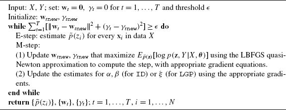

Multi-annotator semi-supervised learning

In order to fully define our model and the specifics of the learning algorithm we did not change the fundamental multi-labeler conditional distribution from that given in Sect. 3.

The gradient with respect to the new parameter ξ is given by:

$$\begin{aligned} \frac{\partial f_\mathtt{LGP}}{\partial\xi} =& \frac{1}{p(\xi |X)}\cdot\frac{\partial p(\xi|X)}{\partial\xi} \sum_i \frac{\sum_{z_i}[\partial p(z_i|\xi,\mathbf{x}_i)/\partial\xi]\prod_t \alpha (y^{(t)}_i;\theta_{t})}{\sum_{z_i}p(z_i|\xi,\mathbf{x}_i)\prod_t \alpha(y^{(t)}_i;\theta_{t})} \\ \frac{\partial f_\mathtt{LGP}}{\partial\theta_{s}} =& \sum _i\frac{\sum_{z_i}p(z_i|\boldsymbol{\xi},\mathbf {x}_i)\prod_{t\backslash s}\alpha(y_i^{(t)};\theta_{t}) \frac{\partial\alpha(y_i^{(s)};\theta_{s})}{\partial\theta _{s}}}{\sum_{z_i}p(z_i|\boldsymbol{\xi},\mathbf{x}_i)\prod_t \alpha(y_i^{(t)};\theta_{t})}, \end{aligned}$$

where we have used $\alpha (y_{i}^{(t)};\theta_{t})=p(y^{(t)}_{i}|\mathbf{x}_{i},z_{i};\theta_{t})$ to simplify the notation. The parameter θ is composed of $\{ {\mathbf{w}}_{t}\}_{t=1}^{T}$ and $\{\gamma_{t}\}_{t=1}^{T}$.

The general learning approach can be summarized in Algorithm 2. The same algorithm can be used for any of the discussed model by replacing the appropriate gradients.

5.3 Prediction

Given a learned model, there exist multiple ways to interpret the problem of making a label prediction given a new data point. Here we focus on inferring the ground-truth for a new data point that was not known during training time (the usual inductive scenario). Specifically, we would like to estimate $p(z_{\mathtt{test}}|X,Y_{\mathcal{ L}};\boldsymbol{\theta})$. This is basically equivalent to performing the E-step as described before and computing $\tilde{p}(z_{\mathtt{test}})$ as in the model-specific E-step.

6 Related problems

The models proposed so far are sufficiently general to tackle problems beyond learning and inferring class labels (along with annotator expertise) in the classical supervised and semi-supervised scenarios. In particular, we briefly describe how the proposed model can be utilized to (1) infer a class label when a new data point is presented and some annotators provide labels for it, (2) how to estimate ground-truth given labels provided by various annotators (no input features), and (3) how to evaluate annotators.

6.1 Including annotator labels at test time

From Eq. (13) we can derive the posterior when not all the annotators provided a label for a data point by computing the appropriate marginal distributions. If annotator k was missing, one can show that the model provides a simple solution:

$$\begin{aligned} p\bigl(z|\bigl\{ y^{t \backslash k}\bigr\} ,\mathbf{x}\bigr)= \frac{\prod_{t \backslash k} p(y^{(t)}|z,\mathbf{x})p(z|\mathbf{x})}{\sum_z \prod_{t \backslash k} p(y^{(t)}|z,\mathbf{x})p(z|\mathbf{x})}, \end{aligned}$$

(29)

which basically ignores the missing annotator. This implies the natural result that if all annotators are missing, we obtain Eq. (7).

6.2 Estimating the ground-truth without observing input data (x)

The presented model provides an expression for estimating the ground-truth even purely from the observed annotations (when the input data has not been observed).

$$\begin{aligned} p\bigl(z|\bigl\{ y^{(t)}\bigr\} \bigr)= \int\prod _t p\bigl(y^{(t)}|z,\mathbf{x}\bigr)p(z|\mathbf {x})dp(\mathbf{x}) \end{aligned}$$

(30)

Since we do have a direct prior p(x), we can rely on sampling. One proposal is to use the previously seen cases (training data) as a good sample for X. Let $\mathcal{ X}_{S}=\{\mathbf{x}_{1},\mathbf{x}_{2},\ldots,\mathbf {x}_{S} \}$, a sample from the random variable X. We can use this sample to compute the posterior by:

$$\begin{aligned} p\bigl(z|\bigl\{ y^{(t)}\bigr\} \bigr)\approx\frac{1}{S}\sum _{s=1}^S p(z|\mathbf {x}_s) \prod_t p\bigl(y^{(t)}|z, \mathbf{x}_s\bigr), \end{aligned}$$

(31)

which can be done easily given a learned model.

6.3 Evaluating annotators

If we knew the ground-truth (for a particular data point), we can straightforwardly evaluate the annotator accuracy. However, this is not the usual case. What if we do not have the ground-truth (it does not exist or is expensive to obtain)? The proposed approach provides a way to evaluate an annotator even without reliance on ground-truth. We can do this by evaluating the following conditional distribution:

$$\begin{aligned} p\bigl(y^{(k)}|\bigl\{ y^{(t \backslash k)}\bigr\} ,\mathbf{x}\bigr)=\frac{p(\{y^{(t)}\} |\mathbf{x})}{p(\{y^{(t \backslash k)}\}|\mathbf{x})} =\frac{\sum_z p(\{y^{(t)}\}|z,\mathbf{x})p(z|\mathbf{x})}{\sum_z p(\{y^{(t \backslash k)}\}|z,\mathbf{x})p(z|\mathbf{x})} \end{aligned}$$

(32)

Note that if the ground-truth is given (along with the input data), the annotators are mutually independent and p(y ^(k)|{y ^(t∖k)},x)=p(y ^(k)|x), as expected.

7 Experimental results

7.1 Supervised setting

In this section, we used several simulated and real data sets to compare the performance of our proposed supervised approach to other baseline and state-of-the-art methods. Our experiments were divided in three parts:

• (I) Performance simulations on UCI data: We tested our algorithm on four publicly available data sets from the UCI Machine Learning Repository (Asuncion and Newman 2007): ionosphere, Cleveland heart, glass, and housing. Since there are no multiple annotations (labels) for these data sets, we artificially generated 5 simulated labelers with different labeler expertise and considered the provided labels as golden ground-truth.

• (II) Modeling labeler’s expertise on a heart motion abnormality detection problem: In this case we perform experiments based on real cardiac data. This data is related to automatic assessment of heart wall motion abnormalities (Qazi et al. 2007). The purpose of this experiment is to measure how well our model learns the labeler’s expertise based on the particular case characteristics (data point features).

• (III) Performance on the breast cancer data set: analogous to (I) but with a real data set extracted for MR digital mammographies and used for classifying regions of interest in the breast into benign and malignant. The cases are labeled by three expert radiologists based on visual inspection of the images. The golden ground-truth was obtained by performing a biopsy in each case. This is quite a rare opportunity where ground-truth actually exists, in particular in the medical domain.

For our proposed multiple labelers method (M.L.), in our comparisons, we considered three different variations that depend on the modeling of p(y|x,z) as described in Sect. 4. M.L.-Gaussian(x) and M.L.-Bernoulli(x) will refer to the models that explicitly depend on x. We will refer as M.L.-Original the original formulation that estimates a parameter σ per labeler in the spirit of Raykar et al. (2009) and Jin and Ghahramani (2003). For further comparisons, we also learn two additional logistic regression classifiers, one using the labelers majority vote as target labels for training (Majority), and the other one concatenates all the labelers’ information by repeating training data points as many times as needed to represent all the labelers (Concatenation).

For both (I) and (II) in Sects. 7.1.1 and 7.1.2 respectively, we randomly divided the data into five equally sized folds (20 % of the data each). For each data set, we repeated the model training five times where we used four of the folds (80 % of the data) for training and one fold for testing. For (III) in Sect. 7.1.3 we used 40 % for training and the remaining 60 % for testing.

7.1.1 Performance simulations on UCI data

We performed experiments on four data sets from the UCI Irvine machine learning data repository (Asuncion and Newman 2007): ionosphere (351,34), Cleveland heart (297,13), glass (214,9), and housing (506,13) (with (number of points, number of features) for each). Since multiple labels for any of these UCI data sets are not available, we need to simulate several labelers with different labeler expertise or accuracy. In order to simulate the labelers, for each data set, we proceeded as follows: first, we clustered the data into five subsets using k-means (Berkhin 2002). Then, we assume that each one of the five simulated labelers i={1,…,5} is an expert on cases belonging to cluster i, where their labeling coincides with the ground-truth; for the rest of the cases (cases belonging to the other four clusters), labeler i makes a mistake 35 % of the times (we randomly switch labels for 35 % of the points). Figures 3 and 4 show the ROC comparisons for different multi-labeler models and baseline logistic regression models for the four data sets. The experimental results demonstrate the power of the proposed approach. We can see that even when the labelers have only slightly better performance than random (around 60 % AUC), our probabilistic models can achieve significantly better performance (around 90 % AUC). These appear to be successfully modeling who is a good labeler for different subsets of training data. Our approaches significantly outperform baseline methods where information from all the labelers is not exploited as appropriately.

Fig. 3

ROC comparison of multi-labeler methods for the UCI data sets glass and Cleveland heart

Fig. 4

ROC comparison of multi-labeler methods for UCI data sets ionosphere and housing

7.1.2 Modeling labeler’s expertise on the AWMA heart data

The automated heart wall motion abnormality (AWMA) detection data consists of 220 clinical cases for which we have ultrasound image sequences (video) of the patient’s heart generated under pharmacological stress (Qazi et al. 2007). All the cases have been labeled at the heart wall segment level by a group of five trained cardiologists indicating whether an abnormal motion is present in the ultrasound video. According to standard protocol, there are 16 LV heart wall segments. Each of the segments were ranked from 1 to 5 according to its movement. For simplicity, we converted the labels to a binary (1 = normal, 2 to 5 = abnormal). For our experiments, we used 24 global and local image features for each node calculated from tracked contours.

Since we have 5 doctor labels but no golden ground-truth (biopsy), we will assume that the majority vote of the 5 doctors are a fair approximation to the true labels. For this experiment we proceeded as follows: after training, we used our model to pick the best labeler for each training data point. Then, we trained a simple logistic regression model using the suggested label. We compared our two proposed models (M.L.-Gaussian(x) and M.L.-Bernoulli(x)) against a baseline model where for each training data point the corresponding labeler is picked randomly among the five available labelers (Random selection).

Figure 5 shows the corresponding ROCs for this experiment. Note that when using the annotator’s labels suggested by our model, a simple logistic regression method clearly outperforms a model trained using labels coming from a labeler picked at random among the five labels available form the annotators. This model has an interesting potential in a medical setting where annotating cases is expensive. The proposed model can rank experts by case and can help decide which annotator is more appropriate to label a given new case.

Fig. 5

ROCs of the three logistic regression models for the cardiac data: M.L.-Gaussian(x), M.L.-Bernoulli(x) and random selection

7.1.3 Performance on the breast cancer data set

Computer-aided detection (CAD) algorithms for mammography are designed to detect suspicious findings in a digitized mammographic image with a high sensitivity. Given a set of descriptive morphological features for a region in an image, the task is to predict whether it is potentially malignant or not. We use a set of mammograms collected from hospitals that generate a biopsy-proven (which provides the golden ground-truth) data set containing 28 positive and 47 negative examples. Each instance is described by a set of 8 morphological features and labeled independently by three doctors. Results are presented in Fig. 6. Note that the results are similar to the ones obtained in Sect. 7.1.1. Our proposed M.L. methods again significantly outperform the baseline methods and each individual annotator even when using a reduced set of training data (only 40 % in this case).

Fig. 6

ROCs for various methods utilized to predict malignancy in the breast cancer data set

7.2 Supervised setting. When some ground-truth is available

In this experiment we try to understand to what extent knowledge of the ground-truth for some of the points can improve the overall model performance. A key motivation for this experiment is that this will allow us to gauge the extent to which the multi-labeler annotator model proposed is optimal (with respect to a model that has access to some or all of the training data ground-truth). For comparison, we utilize the same data sets employed in the previous section, with the exception of the AWMA data for which there was no practical way to collect the ground-truth.

The training algorithm is very similar to that provided in Sect. 3.1, but required a minor change to Eq. (10) to take into account the knowledge of the ground-truth as follows:

$$\begin{aligned} \tilde{p}(z_i) \propto= \mathbf{I}(z_i== \breve{z_i}) \prod_t p \bigl(y^{(t)}_i|\mathbf{x}_i,z_i \bigr)p(z_i|\mathbf{x}_i), \end{aligned}$$

(33)

where $\breve{z_{i}}$ is the ground-truth label for the i-th data point and I is the indicator function returning a value one if the argument is true and 0 otherwise. In order to answer the above questions. We run the modified training algorithm and provided it with various amounts of ground-truth using the Bernoulli conditional distribution case.

7.2.1 UCI Benchmark

Figures 7 and 8 show the algorithm performance for the Bernoulli model (M.L.-Bernoulli) in terms of the AUC when knowledge of (20 %, 40 %, 60 %, 80 %, 100 %) of the ground-truth is available. As a reference point, from the previous section, the performance on the four data sets was (0.83, 0.91, 0.93, and 0.91) for Glass, Cleveland Heart, housing, and ionosphere respectively when no ground-truth is provided. The performance with 20 % ground-truth for the same data sets was (0.83, 0.915, 0.93, 0.88), while for 100 % ground-truth it was (0.92, 0.927, 0.95, 0.90) respectively.

Fig. 7

AUC analysis based on partially known ground-truth for the UCI data sets glass and Cleveland heart

Fig. 8

AUC analysis based on partially known ground-truth for the UCI data sets housing and ionosphere

We can observe that in general, the performance of the multi-labeler model with no ground-truth is very similar to the performance of the model with various amounts of ground-truth. The largest difference was a roughly 10 % performance gain on the glass data when all ground-truth was known. For the rest of the data sets, the difference was around 2 %.

This is to some extent surprising. However, even though 4/5 annotators make mistakes 35 % of the time (for each data point), the annotators are independent of each other² and their combined labels appear to provide sufficient information. This information is efficiently exploited by the multi-labeler model. Independently from the model employed, these results indicate that the information provided by multiple labels about the ground-truth labels is close to maximal.

A secondary observation is the diminishing increase in the AUC as more ground-truth is provided. This is a common property of learning algorithms as most performance improvements normally occur with the first data points (assuming data is presented uniformly at random).

The larger increase in the glass data can be attributed to its size. As the smallest of the data sets, the information per ground-truth label is likely larger than for the rest of the data sets. However, this is by no means the only possible explanation and other factors such as the properties of the data set themselves are likely to play an important role. The performance of M.L.-Gaussian and M.L-Bernoulli were qualitatively similar, as in previous experiments.

These experiments are useful for showing that the model can be adjusted appropriately and is flexible enough to take advantage of existing ground-truth labels. While they elucidate the general benefits expected from injecting ground-truth into the model, we must also remark that the true benefit derived from accuracy gains relative to the ground-truth acquisition effort (cost) is in general application dependent. For example, we expect small gains in accuracy in the medical diagnosis domain to be more valuable to justify larger investment efforts.

7.2.2 Breast cancer data set

The results for the breast cancer data set for varying knowledge of ground-truth is shown in Fig. 9. The results are similar to that of the glass data and consistent with the rest of the data set. The improvement from an AUC of 0.82 (previous section result) to an AUC of 0.88 with 20 % of the ground-truth is considerable and illustrates the ability of the algorithm to work with partial ground-truth. This relatively large increase may be attributed to the small data set size and possibly to the accuracy of the radiologists (although their accuracy has not been estimated). The AUC increase as more ground-truth is provided is smaller but still quite large relative to the previous experiments. One could hypothesize that this result maybe evidence of unreliable annotators, but this verification goes beyond this experimental setup.

Fig. 9

ROC analysis based on partially known ground-truth for breast cancer

7.3 Spammers and adversarial annotators

In the next set of experiments we explore (1) whether the proposed model allows for detecting spammers and adversarial annotators; and (2) how sensitive the proposed model is with respect to spammers and adversarial annotators. The definition of a spammer or alternatively an adversarial annotator can vary. In the context of this paper, we let spammers be those annotators that assign labels to data points with little regard to the input (similar to assigning labels uniformly at random), while adversarial annotators are those annotators that tend to assign the incorrect label to the data with high probability. It is possible to come up with more sophisticated annotator behaviors (including collusion behavior), but this will not be considered as part of the paper’s scope.

There are many reasons for trying to achieve this. These annotators could potentially impact negatively the learning process. In practice, a motivation for attempting to identify these annotators is to exclude them from the learning process early on or treat them differently than the rest (potentially to uncover their true nature or for analysis purposes). Further, in order to understand the limits of the model, we also explore how the model performs with respect to increasing spammer and adversarial influence.

7.3.1 Experimental setup

We used the Breast Cancer, Atrial Fibrillation (see Sect. 7.4.3 for a description), Glass, ionosphere, and housing data sets to evaluate the spammer adversarial annotators. We employ the strategy proposed in Sect. 6.3 which utilizes the conditional distribution of an annotator label given other annotator labels as formalized in Eq. (32). This takes into consideration that the ground-truth is not known, as studied in our general setting (clearly, if the ground truth were known, this task would be straightforward).

This conditional probability can be seen a measure of how much an annotator’s label, for a given data-point, can be correctly inferred from that of other annotators. Since Eq. (32) is defined for a single data point, we utilize a spammer score that involves computing the negative sum of logs of the above measure across all data-points:

$$ S_{k} = -\sum_i \log p \bigl(y_i^{(k)}|\bigl\{ y_i^{(t \backslash k)}\bigr\} ,\mathbf{x}_i\bigr) $$

(34)

This is comparable with the negative log-likelihood measure frequently utilized in other learning tasks. Thus, if an annotator’s labels are difficult to infer based on the labels from the rest of the annotator, then the conditional probabilities above will be generally low. The lower these probabilities the larger the score; thus, a large spammer score is indicative of an annotator that is less predictable. However, note that an annotator that is consistently contradicting other annotators would, in general, be quite predictable. In fact, his/her labels could provide valuable information about the task. These aspects are experimentally considered in the next sections.

While we use a global score to help determine whether an annotator is e.g., a spammer and to measure model sensitivity, alternatively we could use a spammer probability (i.e., Eq. (32)) on a point-by-point basis. We use the former strategy since it is more appropriate/fundamental for a first experimental investigation. The latter option is plausible because in the proposed model the annotator effectiveness is dependent on the input data point observed. That is, for some data points one annotator may be considered more reliable than another while for other data points this situation could be reversed. A more sophisticated experimental setup is necessary to evaluate model sensitivity in the second setting where annotator spammer/adversarial tendencies vary.

In our experiments we utilized the same annotators and their corresponding labels as in the supervised setting above. In addition, we add annotators with various levels of adversarial strength p _a . In order to evaluate our approach in a controlled manner, we define these annotators as perfect annotators (as given by the ground-truth) with a stochastic component consisting of a label-flip with probability p _a . Thus, an adversarial annotator with p _a =α correspond to an annotator that has knowledge of the correct label but flips it with probability α independently for each data point presented. In order to address the input-specific spammer/adversarial behavior we could look at the point-by-point values (Eq. 32) necessary to calculate the spammer score, but this was not our intended scope.

In terms of our definitions of spammer and adversarial annotators above, a perfect spammer will have p _a =0.5, while an adversary will have p _a =1.

7.3.2 Experiments and discussion

In order to illustrate the approach, we first use the Breast Cancer data set. Consider Fig. 10, where various data points are plotted against the value of the conditional probability used for evaluation (Eq. (32)) for each annotator. In the first graph (left), all the annotators remain the same, and a fourth annotator with p _a =0.4 is introduced in the data set. We can observe that the new annotator generally obtains a lower conditional probability value compared with the rest, indicating that it is relatively more difficult to predict the label of this annotator. In the second graph (right), we use the three original annotators but flip the label of the first annotator with p _a =0.4. Note that its conditional probability value decreased noticeably relative to the previous graph. The impact of spammer annotators is clear in both cases, partly because of the large value of p _a utilized. We can also observe the larger score assigned to those annotators that have altered their labels.

Fig. 10

Probability corresponding to Eq. (32) for evaluating annotators for each data point: (left) one adversary introduced with corresponding labels randomly flipped with probability p _a =0.4, (right) annotator 1 labels randomly flipped with probability p _a =0.4

This illustrates the effect of this type of label changes on the proposed conditional probability in Eq. (32). In the rest of the experiments we utilize this basic concept in order to evaluate spammer and adversarial annotators and their effect in various manners.

In the next experiment we measure the combined impact of the number of spammer and adversarial annotator and the strength of p _a in their spammer score and the score of various non-spammer/non-adversarial annotators (the original data set annotators). In Fig. 11 we plot the score of all the annotators while varying p _a . This is done for the case of one and three spammer/adversarial annotators (top) and nine spammer/adversarial annotators (bottom-left).

Fig. 11

Breast cancer data set. Scores for each annotator when 1 (top-left), 3 (top-right) and 9 (bottom-left) adversaries are introduced. AUC for various levels of p _a and different numbers of adversarial annotators (bottom-right)

In this graph we can observe various properties of the approach. Spammers are in the center of the graph around p _a =0.5, while the adversaries (as defined above) are on the right of the graph around p _a =1. The scores for the non-adversarial/non-spammer annotators are fairly constant across all values of p _a . This indicates that the scoring scheme is robust to the number of adversaries and the strength of p _a .

It can also be noted that the score curves for the spammers/adversarial annotators (red bars) are symmetric about p _a =0.5, where the maximum occurs. This is consistent with the notion that a completely random annotator provides the least amount of information to the model. That is, the score predicts that spammers are expected to be the least helpful to the model in the settings considered above.

On the other hand, a perfect annotator would have a very low spammer score (as expected), but an annotator that provides labels perfectly opposite to the ground-truth would also have a very low spammer score. This agrees with the notion that effective models can learn to flip the training/predicted labels based on enough evidence from the training data. Clearly, a perfectly opposite annotator provides a lot of information about the true label. We defined an adversarial annotator as one that provides labels perfectly opposite to the ground-truth. These results clearly suggest that the spammer score can capture the idea that these annotators can indeed be helpful for learning.

In order to further validate the above, we conducted experiments to measure performance under all of the previous experimental conditions. In Fig. 11 (bottom) we measure how the AUC is affected for varying levels of p _a and for various numbers of spammer and adversarial annotators. We can see how the AUC can remain at the highest level under a varied amount of spammer and adversarial influence. Interestingly, there appears to be a value for p _a where the AUC starts to degrade quickly. The speed of the degradation is larger when more adversarial annotators are present. The number of adversarial annotators also influences the critical value of p _a where the AUC degradation starts to occur in a significant manner.

These experiments were re-run for the other data sets. The equivalent graphs are shown in Figs. 12, 13, 14 and 15. While we utilized a different number of spammer/adversarial annotators, the results are consistent throughout and strengthen the validity of the approach for evaluating annotators. In particular, the interaction between p _a , the number of spammer/adversarial annotators, and the way in which the AUC suffers is remarkably consistent across data sets.

Fig. 12

Atrial fibrillation data set. Scores for each annotator when 1 (left) and 3 (right) adversaries are introduced. AUC for various levels of p _a and different numbers of adversarial annotators (bottom-center)

Fig. 13

Glass data set. Clockwise from top-left corner, scores for each annotator when 1, 4, and 10 adversaries are introduced. AUC for various levels of p _a and different numbers of spammer and adversarial annotators (bottom-right)

Fig. 14

Ionosphere data set. Scores for each annotator when 1, 3, and 9 adversaries are introduced. AUC for various levels of p _a and different numbers of spammer and adversarial annotators (bottom-right)

Fig. 15

Housing data set. Scores for each annotator when 1, 3, and 9 adversaries are introduced. AUC for various levels of p _a and different numbers of spammer and adversarial annotators (bottom-right)

Regarding the spammer score, we observed a consistent ability of the approach to distinguish spammers from clearly accurate and adversarial annotators. Uniformly unreliable annotators can be confused with a spammer as expected. On the other hand, the approach cannot accurately distinguish between a consistently good annotator and an adversarial annotator that consistently labels opposite to the ground-truth. This is not surprising, as the spammer scores measures how predictable annotator labels are relative to known labels for the same data points. Clearly an annotator that consistently labels opposite to ground truth is predictable from other sufficiently consistent annotators.

Note also that the score is dependent on w _t and γ _t . Thus, alternatively we can use these parameters to calculate the annotator uncertainty quantities σ _t (x) or η _t (x). However, these quantities do not take into account the potentially known labels given by other annotators to evaluate one given annotator (for a specific data point). Equation (32) does address this; as an example, if annotators provided an unexpected label for a data point, then the probability that the evaluated annotator will provide a surprising label is reduced.

Regarding the AUC experiments, we observed a clear difference in the effect of spammers vs. the effect of adversarial annotators on the test AUC. While the model can consistently withstand the effect of spammers even when they triple the number of non-spammers, the model is less resistant to adversarial annotators. From all the results above, we observed that N perfectly adversarial annotators are generally sufficient to decrease the AUC to 0.5, where N is the number of reasonably accurate annotators. This is not surprising, and is quite likely to occur due that, without additional information, a large enough number of annotators consistently labeling each data point with the opposite label will make learning models predict the incorrect label. In all our tasks, the regular annotators are clearly not perfect and sometimes provide an incorrect label.

7.4 Semi-supervised setting

In this section, we compare our semi-supervised multi-annotator model, the logistic graph Laplacian prior (logistic-GP), against baseline methods on a number of UCI Machine Learning Repository (Frank and Asuncion 2010) benchmark data with simulated labelers, and real data sets. In our experiments we show the results for our logistic + graph prior (LGP). Compared to the ID model, this has the clear advantage of being able to make use of the unlabeled data.

We compare our method against the following baselines, testing different aspects of our model: (1) standard logistic regression classifier trained on labels from the annotators’ majority vote (we call this majority vote), (2) standard logistic regression classifiers trained on labels from each annotator (annotator t), (3) a supervised multi-labeler logistic regression model version of our approach with the variance not a function of the input x (ML original), which is similar in spirit to that of Jin and Ghahramani (2003), Raykar et al. (2009), and (4) a semi-supervised support vector machine (SVM) classifier with a linear kernel from SVM-light³ (SVM-light) trained on labels from the annotators’ majority vote. The parameters in SVM were tuned on a validation set using grid search. We compare against methods (1), (2) and (3) to test the advantage of learning from unlabeled data. In addition, by comparing with (1), (2) and (4), we also test whether or not learning from multi-labelers is better than just from one labeler alone. Against method (3), we also test the effect of taking the variance of an annotator’s accuracy σ(x) (in labeling across different observations) into account for classification performance.

7.4.1 UCI Benchmark data

Again, we first performed experiments on various data sets from the UCI machine learning data repository (Frank and Asuncion 2010): ionosphere (351,34), dim (4192,14, housing (506,13), Pima (768,8), BUPA (345,6), Wisconsin breast cancer 24 (155,32), and Wisconsin breast cancer 60 (110,32). Since multiple annotations for any of these UCI data sets are not available, we needed to simulate several labelers with different labeler expertise or accuracy.

In order to simulate the labelers, for each data set, we proceeded as follows: first, we clustered the data into five subsets using k-means (Berkhin 2002). As before, we assume that each one of the five simulated labelers i,i=1,…,5, is an expert on cases belonging to cluster i, where their labeling coincides with the ground-truth; for the rest of the cases (cases belonging to the other four clusters), labeler i makes a mistake 35 % of the time (we randomly switch labels for 35 % of the data samples). Figure 16 displays plots of the stratified five-fold cross-validated accuracies of the different methods on these UCI data sets as the proportion of the training data that is labeled is increased. These results show that our semi-supervised multi-labeler based on the logistic and Laplacian prior (logistic-GP) has the best accuracies in almost all proportions of labeled training data cases for the data sets.

Fig. 16

Accuracies for the various UCI data sets for different proportion of labels (in the range [0.1,1]) in the training data. Results show averages for five randomized splits of training (labeled and unlabeled) and test sets, with cross-validation

Logistic-GP is designed to handle label scarcity and this provided a clear advantage when few labels were given. These experiments in general confirm these advantages. Logistic-GP can also model input-dependent annotator specific expertise and this allowed it to keep performing well even when more labels were given and the prior was not as important.

More specifically, we believe that the proposed logistic-GP approach performed better than SVM-Light because it was able to take into account multiple labelers’ expertise. It outperformed the fully supervised methods because it was able to learn from unlabeled data as well. We believe it performed better than M.L.-Original because the method is semi-supervised and also because it can take advantage of modeling the variance of an annotator’s accuracy (σ(x)) in labeling across different observations. Finally, logistic-GP also performed better than M.L.-Gaussian, which like logistic-GP can take advantage of modeling input-dependent annotator reliability. Particularly, when the training data portion was small the difference was more pronounced since logistic-GP benefited from the proposed graph prior to more efficiently utilize the available data when labels were scarce. This gap was reduced when more labels were available since the prior becomes less relevant.

We conclude with one additional observation. M.L.-Original often performs reasonably well, but in very few experiments it performed poorly. Even though this experiment was not primarily intended to test M.L.-Original, Fig. 16(d) provides a clear instance of this situation. From inspecting the estimated parameters, we realized that the learning algorithm for this model is consistently converging to a solution where almost equal trust is placed on each labeler. Basically M.L.-Original could not effectively learn the input-specific reliability for each annotator. Recall that M.L.-Original estimates individual annotator accuracy but, unlike the proposed approaches, this accuracy is not input-dependent. For the Pima data set, this was a very poor solution, worse than trusting a single annotator and ignoring the rest, as the graph also shows.

7.4.2 AWMA cardiac data

Again we used the Automatic Wall Motion Abnormality Detection (AWMA) data. Similarly, only for evaluation purposes, since we have five doctor labels but no ground truth we will assume that the majority vote of the five doctors are a fair approximation to the true labels. We applied stratified five-fold cross-validation to evaluate our results.

Figure 17 shows the average five-fold cross-validated accuracies of our method against the different baselines as we increase the proportion of training data labeled by annotators. Since this data is actually comprised of several classification problems (one for each segment), we report the average (top) and the standard deviation results (bottom). We observe that our model outperforms all the baseline methods for this data in terms of average accuracies. This is because we have extra unlabeled information helping us improve our performance and we take multiple annotator labels into account in learning our classifier.

Fig. 17

Accuracies for the AWMA cardiac data with different percentage of the training data labeled, averaged over five randomized train/test set selections

Accuracies do not reveal the trade-off between the true positive rate and false alarm rate. Here, we also show the average ROC results for our model compared to the different baselines. Different from the experiments with supervised cases, here we set the proportion of training points to 20 %, 50 % and 100 %. The results are shown in Fig. 18. The logistic-GP (LGP) model outperforms the others when there are only few labeled points (at 20 % of the training data). Logistic-GP is slightly better than semi-supervised SVM (SVM-light) and almost equal in performance to ML original when using all 100 % labeled (i.e. no extra unlabeled information). SVM-light performed reasonably well and close to our method when there are a few labels because the ground-truth for this data is based on the majority vote of the annotators which is what SVM-light uses as labels for training. Interestingly, even though logistic-GP does not have this ground-truth label, but labels from all five labelers, it outperformed SVM-light. Note, that when all labels are available, logistic-GP together with ML original, both of which learn from multiple labelers, outperformed the others which are simply based on the majority label (ground-truth) or labels from single annotators.

Fig. 18

ROC comparison with (a) 20 %, (b) 50 % and (c) 100 % of the training data labeled for the AWMA data using multi-label semi-supervised learning and competing methods. The curves show averages over five randomized runs

7.4.3 Atrial fibrillation medical text understanding data

We additionally tested the different methods on medical text data related to automatic detection of Atrial Fibrillation (cardiac arrhythmia of abnormal heart rhythm) from unstructured medical text. This is a representative example of a common and very relevant area in medical text analysis. The goal is to ascertain or infer that a piece of text (a sentence, passage, or document) refers to a particular topic or concept, in this case atrial fibrillation (AF).

The AF data consists of valid electronic medical records (EMR) from various medium/large-size hospitals. The data points from this data set are divided at the passage level. A passage is a sequence of word/tokens extracted from a document. Thus, each training point represents a passage-based observation.

The AF data set consists of a set of 1057 passages from a medical database containing a variety of different medical records: discharge notes, visit notes, bills, etc. The passages have been annotated by an expert labeler (nurse abstractor) and four non-expert labelers. Each passage is labeled into one of two categories: whether the passage is relevant in determining (or providing clear evidence) that the patient has a history of AF or not. The text to be analyzed is represented based on a combination of the document meta-data (document type, date, formatting information) and contextual information. For a passage of interest, the context is defined as the section the passage is in, the distribution of words in the passage, and the relationships between these words. When a document is analyzed, two main elements are identified: (1) document meta-data and (2) the actual text in the document (the content). These are represented as a vector of real numbers. In this data set, 741 out of 1057 are annotated by 5 doctors and each sample has 323 features. We set 741 data points as training samples, and 316 data points for testing.

The experiments, summarized in Fig. 19, show that when 20 % of the annotator labels are available most approaches perform poorly. However, the two types of multi-labeler models introduced in this paper were able to use the available labels better compared to SVM-Light and majority voting. The performance of models trained on individual labels was close to random. Majority also performed quite poorly in these experiments. We have not fully characterized the behavior of majority voting with respect to the performance of individual annotators. We believe this can happen when the most common label (from the model’s viewpoint) is not consistent across data points. Across all our experiments we observe that majority voting often performs reasonably well. However, there is no guarantee that majority voting is always better than individual annotators on the test set.

Fig. 19

ROC comparison with (a) 20 %, (b) 50 % and (c) 100 % of the training data labeled for the Atrial Fibrillation data using multi-label semi-supervised learning and competing methods. The curves show averages over five randomized runs

At 50 % logistic-GP clearly excels compared to the other models including the other multi-labeler model (but which does not take into account the semi-supervised nature of the problem). The difference between logistic-GP and the rest is noticeable.

When 100 % of the available labels are used, M.L.-Original’s performance was closer to that of logistic-GP, but still the models are a significant distance apart. This was a surprise at first, as in the previous data sets the performance between these two models, at the 100 % level, was much closer. A reason for this difference is likely because this data set fits the semi-supervised setting better than the previous data sets since a larger proportion of data points are labeled only by some annotators. SVM-light made major gains, but its performance was still not comparable with the multi-labeler models, while majority voting suffered a large performance degradation which we did not investigate further.

7.4.4 IMDB rating data

To conclude the semi-supervised experiments we utilized the Internet Movie Database (IMDB) Rating data. This is a subset of the IMDB data.⁴ The input representation consists of identifier features for actors, directors, languages, and genres. Since many movies do not have all the information necessary to build these features, we considered the 3189 movies with the features most commonly present and rated by the 200 most common on-line raters. Each movie in the generated subset was represented by 789 features. We divided this data set into 900 samples for training and 2289 samples for testing. From the data we used the top-10 critical rating information, basically an equivalent to expert rating labels, to establish our ground-truth labels (using the majority rating for simplicity).

Figure 20 shows our results. Since for this data set the labeling is very sparse and the annotators labeled a clearly non-overlapping set of movies, we did not simulate the amount of annotator labels as we did for the other data sets, instead we used all the labels provided by the 200 annotators. Also, since we have this many annotators, it is not practical to show all the classifiers trained by every individual; thus, we provide the best and worst individual classifiers.

Fig. 20

ROC curve for the IMDB data set comparing logistic-GP with competing methods

Logistic-GP and ML-original were, as expected, the best performers, with the first clearly improving upon the second. As in the previous experiments SVM-light was superior than majority voting but its performance was still far from that of the multi-labeler models. The best and worst annotators were markedly different in their performances, and majority voting was slightly better than the best annotator.

The sparsity of the annotator labels makes this data set a great fit for the semi-supervised approach presented in this paper as there are a considerable number of cases for which the annotators did not label the movies and annotator similarities were likely exploited to produce such an performance increase with respect to the supervised multi-labeler model.

8 Conclusion

Traditionally, supervised learning relies on a single labeler playing the role of a teacher providing the necessary supervision. However, the increasing availability of more annotators for certain domains, the difficulty of obtaining ground truth (such as in cancer detection in medical images), and/or the subjectivity of labeling (such as product ratings), lead to the growing importance of studying supervised learning when there are multiple annotators whose labels may be unreliable. A distinguishing factor in this paper, in contrast to previous approaches, is that we do not assume that the reliability of annotators is the same across all data. In many cases, annotator knowledge can fluctuate considerably depending on the specific input instance observed. This is the common case when everyone knows something about the problem domain, but everyone may know different aspects of the same problem (rarely does someone know everything).

In this paper, we developed a probabilistic model for learning a classifier from multiple annotators, where the reliability of the annotators vary on the annotator and the data that they observe. Our approach allows us to provide estimates for the true labels given new instances and also provide the expertise variability for each annotator across the domain task. Our experiments on real and simulated multi-labeler data show that the expertise of annotators do vary across data and that our model provides better classification performance over various forms of data preprocessing (majority vote or concatenation of the labels provided by all the annotators), and more importantly improves the results over the model that ignores the effect of variable expertise across instances.

In addition to learning from multiple annotator information, we also allow our model to learn from unlabeled data in a semi-supervised learning scenario. This ability is important in many common domains where there exist large amounts of unlabeled data. In addition to utilizing the topology of the input space, like it is often done by semi-supervised learning algorithms (Belkin et al. 2004; Blum and Chawla 2001; Corduneanu and Jaakkola 2005; Krishnapuram et al. 2005), the proposed model can also learn from the implicit relationships between different annotators, based on their labeling patterns. We are not aware of other models that can take advantage of these aspects. Experiments show that our model, taking advantage of the extra information from the unlabeled data, outperforms approaches that only learn from labeled data. Moreover, learning from multiple annotators improves classification performance over standard single annotator supervised and semi-supervised classifiers.

We have further provided an analysis of the proposed approach in terms of the resulting decision boundary properties for a Bernoulli and for a Gaussian conditional annotator model. We showed how the model is suitable for handling missing annotators, for estimating the ground-truth, and for evaluating annotators when the ground-truth is not available. This was done in the formal context of probabilistic inference once the correct conditional distribution of interest were learned.

References

Asuncion, A., & Newman, D. (2007). UCI machine learning repository. URL http://www.ics.uci.edu/~mlearn/MLRepository.html.
Belkin, M., Matveeva, I., & Niyogi, P. (2004). Regularization and semi-supervised learning on large graphs. In Proceedings of the workshop on computational learning theory (pp. 624–638). San Mateo: Morgan Kaufmann.
Berkhin, P. (2002). Survey of clustering data mining techniques (on-line). URL http://www.ee.ucr.edu/~barth/EE242/clustering-survey.pdf.
Blitzer, J., Crammer, K., Kulesza, A., Pereira, F., & Wortman, J. (2008). Learning bounds for domain adaptation. In Advances in neural information processing systems (Vol. 20, pp. 129–136). Cambridge: MIT Press.
Blum, A., & Chawla, S. (2001). Learning from labeled and unlabeled data using graph mincuts. In International conference on machine learning (pp. 19–26). San Mateo: Morgan Kaufmann.
Corduneanu, A., & Jaakkola, T. S. (2005). Distributed information regularization on graphs. In Advances in neural information processing systems (Vol. 17, pp. 297–304). Cambridge: MIT Press.
Cover, T., & Thomas, J. (1991). Elements of information theory. New York: Wiley Interscience.
Crammer, K., Kearns, M., & Wortman, J. (2008). Learning from multiple sources. Journal of Machine Learning Research, 9, 1757–1774.
Dawid, A. P., & Skeene, A. M. (1979). Maximum likelihood estimation of observed error-rates using the EM algorithm. Applied Statistics, 28, 20–28.
Dekel, O., & Shamir, O. (2009). Good learners for evil teachers. In Proceedings of the 26th annual international conference on machine learning (pp. 233–240). New York: ACM.
Dempster, A., Laird, N., & Rubin, D. (1977). Maximum likelihood estimation from incomplete data. Journal of the Royal Statistical Society B 39(1).
Donmez, P., & Carbonell, J. G. (2008). Proactive learning: cost-sensitive active learning with multiple imperfect oracles. In Conference on information and knowledge management (pp. 619–628). New York: ACM.
Frank, A., & Asuncion, A. (2010). UCI machine learning repository. University of California, Irvine, School of Information and Computer Sciences. URL http://archive.ics.uci.edu/ml.
Howe, J. (2008). Crowdsourcing: why the power of the crowd is driving the future of business, 1st edn. New York: Crown Publishing Group.
Hui, S. L., & Zhou, X. H. (1998). Evaluation of diagnostic tests without a gold standard. Statistical Methods in Medical Research, 7, 354–370.
Jin, R., & Ghahramani, Z. (2003). Learning with multiple labels. In Advances in neural information processing systems (pp. 897–904).
Kasneci, G., Gael, J. V., Stern, D., & Graepel, T. (2011). CoBayes: Bayesian knowledge corroboration with assessors of unknown areas of expertise. In Conference on web search and data mining (pp. 465–474).
Krishnapuram, B., Williams, D., Xue, Y., Hartemink, A., Carin, L., & Figueiredo, M. (2005). On semi-supervised classification. In Advances in neural information processing systems (pp. 721–728). Cambridge: MIT Press.
Nocedal, J., & Wright, S. (2003). Numerical optimization (2nd ed.). Berlin: Springer.
Paquet, U., Van Gael, J., Stern, D., Kasneci, G., Herbrich, R., & Graepel, T. (2010). Vuvuzelas and active learning for online classification. In NIPS workshop on computational social sciences and the wisdom of crowds.
Qazi, M., Fung, G., Krishnan, S., Rosales, R., Steck, H., Rao, B., Poldermans, D. D., & Chandrasekaran, D. (2007). Automated heart wall motion abnormality detection from ultrasound images using Bayesian networks. In Proceedings of the 20th international joint conference on artificial intelligence (pp. 519–525).
Raykar, V. C., & Yu, S. (2011). Ranking annotators for crowdsourced labeling tasks. In Advances in neural information processing systems (pp. 1809–1817). Cambridge: MIT Press.
Raykar, V. C., Yu, S., Zhao, L. H., Jerebko, A., Florin, C., Valadez, G. H., Bogoni, L., & Moy, L. (2009). Supervised learning from multiple experts: whom to trust when everyone lies a bit. In Proceedings of the 26th annual international conference on machine learning (pp. 889–896).
Sheng, V. S., Provost, F., & Ipeirotis, P. G. (2008). Get another label? Improving data quality and data mining using multiple, noisy labelers. In Proceedings of the 14th ACM SIGKDD international conference on knowledge discovery and data mining (pp. 614–622). New York: ACM.
Smyth, P., Fayyad, U., Burl, M., Perona, P., & Baldi, P. (1994). Inferring ground truth from subjective labeling of Venus images. In Advances in neural information processing systems (pp. 1085–1092).
Snow, R., O’Connor, B., Jurafsky, D., & Ng, A. Y. (2008). Cheap and fast—but is it good?: evaluating non-expert annotations for natural language tasks. In Proceedings of the conference on empirical methods in natural language processing, association for computational linguistics, EMNLP ’08, Stroudsburg, PA, USA (pp. 254–263).
Sorokin, A., & Forsyth, D. (2008). Utility data annotation with Amazon Mechanical Turk. In CVPR workshop on Internet vision (pp. 1–8).
Spiegelhalter, D. J., & Stovin, P. (1983). An analysis of repeated biopsies following cardiac transplantation. Statistics in Medicine, 2(1), 33–40.
Welinder, P., Branson, S., Belongie, S., & Perona, P. (2011). The multidimensional wisdom of crowds. In Advances in neural information processing systems.
Yan, Y., Rosales, R., Fung, G., & Dy, J. (2010a). Modeling annotator expertise: learning when everybody knows a bit of something. In International conference on artificial intelligence and statistics (pp. 932–939).
Yan, Y., Rosales, R., Fung, G., & Dy, J. (2010b). Modeling multiple annotator expertise in the semi-supervised learning scenario. In Conference on uncertainty in artificial intelligence (pp. 674–682).
Zhou, D., Bousquet, O., Lal, T. N., Weston, J., & Schölkopf, B. (2004). Learning with local and global consistency. In Advances in neural information processing systems (Vol. 16, pp. 321–328). Cambridge: MIT Press.
Zhu, X. (2006). Semi-supervised learning literature survey (Technical Report TR-1530). Computer Sciences Department, University of Wisconsin Madison. URL http://www.cs.wisc.edu/~jerryzhu/pub/ssl_survey.pdf
Author information
Authors and Affiliations
Corresponding author
Additional information
Editors: Winter Mason, Jennifer Wortman Vaughan, and Hanna Wallach.
Rights and permissions
About this article
Cite this article
Yan, Y., Rosales, R., Fung, G. et al. Learning from multiple annotators with varying expertise. Mach Learn 95, 291–327 (2014). https://doi.org/10.1007/s10994-013-5412-1
Received:
Accepted:
Published:
Issue Date:
DOI: https://doi.org/10.1007/s10994-013-5412-1