On the Methodological Framework of Composite Indices: A Review of the Issues of Weighting, Aggregation, and Robustness

Abstract

In recent times, composite indicators have gained astounding popularity in a wide variety of research areas. Their adoption by global institutions has further captured the attention of the media and policymakers around the globe, and their number of applications has surged ever since. This increase in their popularity has solicited a plethora of methodological contributions in response to the substantial criticism surrounding their underlying framework. In this paper, we put composite indicators under the spotlight, examining the wide variety of methodological approaches in existence. In this way, we offer a more recent outlook on the advances made in this field over the past years. Despite the large sequence of steps required in the construction of composite indicators, we focus particularly on two of them, namely weighting and aggregation. We find that these are where the paramount criticism appears and where a promising future lies. Finally, we review the last step of the robustness analysis that follows their construction, to which less attention has been paid despite its importance. Overall, this study aims to provide both academics and practitioners in the field of composite indices with a synopsis of the choices available alongside their recent advances.

1 Introduction

In the past decades, we have witnessed an enormous upsurge in available information, the extent and use of which are characterised by the founder of the World Economic Forum as the ‘Fourth Industrial Revolution’ (Schwab 2016, para. 2). While Schwab focuses on the use and future impact of these data—ranging from policy and business analysis to artificial intelligence—one of the key underlying points is that this enormous and exponential increase in available information hides another issue: the need for its interpretation and consolidation. Indeed, an ever-increasing variety of information, broadly speaking in the form of indicators, increases the difficulty involved in interpreting a complex system. To illustrate this, consider for example a phenomenon like well-being. In principle, it is a very complex concept that is particularly difficult to capture with only a single indicator (Decancq and Lugo 2013; Decancq and Schokkaert 2016; Patrizii et al. 2017). Hence, one should enlarge the range of indicators to encompass all the necessary information on a matter that is generally multidimensional in nature (Greco et al. 2016). However, in such a case, it would be very difficult for the public to understand ‘well-being’ by, say, identifying common trends among several individual indices. They would understand a complex concept more easily in the form of a sole number that encompasses this plethora of indicators (Saltelli 2007). Reasonably, this argument may raise more questions than it might answer. For instance, how would this number be produced? Which aspects of a concept would it encompass? How would they be aggregated into the form of a simple interpretation for the public and so on? This issue, and the questions that it raises, introduce the concept of ‘composite indicators’.

Defining ‘composite’ (sometimes also encountered as ‘synthetic’) indicators should be a straightforward task given their widespread use nowadays. Even though it appears that there is no single official definition to explain this concept, the literature provides a wide variety of definitions. According to the European Commission’s first state-of-the-art report (Saisana and Tarantola 2002, p. 5), composite indicators are ‘[…] based on sub-indicators that have no common meaningful unit of measurement and there is no obvious way of weighting these sub-indicators’. Freudenberg (2003, p. 5) identifies composite indicators as ‘synthetic indices of multiple individual indicators’. Another potential definition provided by the OECD’s first handbook for constructing composite indicators (Nardo et al. 2005, p. 8) is that a composite indicator ‘[…] is formed when individual indicators are compiled into a single index, on the basis of an underlying model of the multi-dimensional concept that is being measured’. This list of definitions could continue indefinitely. By pooling them together, a common pattern emerges and relates to the central idea of the landmark work of Rosen (1991). Essentially, a composite indicator might reflect a ‘complex system’ that consists of numerous ‘components’, making it easier to understand in full rather than reducing it back to its ‘spare parts’. Although this ‘complexity’, from a biologist’s viewpoint, refers to the causal impact that organisations exert on the system as a whole, the intended meaning here is astonishingly appropriate for the aim of composite indicators. After all, Rosen asserts that this ‘complexity’ is a universal and interdisciplinary feature.

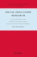
Despite their vague definition, composite indicators have gained astounding popularity in all areas of research. From social aspects to governance and the environment, the number of their applications is constantly growing at a rapid pace (Bandura 2005, 2008, 2011). For instance, Bandura (2011) identifies over 400 official composite indices that rank or assess a country according to some economic, political, social, or environmental measures. In a complementary report by the United Nations’ Development Programme, Yang (2014) documents over 100 composite measures of human progress. While these inventories are far from being exhaustive—compared with the actual number of applications in existence—they give us a good understanding of the popularity of composite indicators. Moreover, a search for ‘composite indicators’ in SCOPUS, conducted in January 2017, shows this trend (see Fig. 1). The increase over the past 20 years is exponential, and the number of yearly publications shows no sign of a decline. Moreover, their widespread adoption by global institutions (e.g. the OECD, World Bank, EU, etc.) has gradually captured the attention of the media and policymakers around the globe (Saltelli 2007), while their simplicity has further strengthened the case for their adoption in several practices.

Fig. 1

Results for ‘composite indicators’ on SCOPUS for the period 1997–2016

Nevertheless, composite indicators have not always been so popular, and there was a time when considerable criticism surrounded their use (Sharpe 2004). In fact, according to the author, their very existence was responsible for the creation of two camps in the literature: aggregators versus non-aggregators. In brief,¹ the first group supports the construction of synthetic indices to describe an overall complex phenomenon, while the latter opposes it, claiming that the final product is statistically meaningless. While it seems idealistic to assume that this debate will ever be resolved (Saisana et al. 2005), it quickly drew the attention of policymakers and the public. Sharpe (2004) describes the example of the Human Development Index (HDI), which has received a vast amount of criticism since its creation due to the arbitrariness of its methodological framework (Ray 2008). However, it is the most well-known composite index to date. Moreover, it led the 1998 Nobel Prize-winning economist A. K. Sen, once one of the main critics of aggregators, to change his position due to the attention that the HDI attracted and the debate that it fostered afterwards (Saltelli 2007). He characterised it as a ‘success’ that would not have happened in the case of non-aggregation (Sharpe 2004, p. 11). Seemingly, this might be considered as the first win for the camp of aggregators. Nevertheless, the truth is that we are still far from settling the disputes and the criticism concerning the stages of the construction process (Saltelli 2007).

This is natural, as there are many stages in the construction process of a composite index and criticism could grow simultaneously regarding each of them (Booysen 2002). Moreover, if the procedure followed is not clear and reasonably justified to everyone, there is considerable room for manipulation of the outcome (Grupp and Mogee 2004; Grupp and Schubert 2010). Working towards a solution to this problem, the OECD (2008, p. 15) identifies a ten-step process, namely a ‘checklist’. Its aim is to establish a common guideline as a basis for the development of composite indices and to enhance the transparency and the soundness of the process. Undeniably, this checklist aids the developer in gaining a better understanding of the benefits and drawbacks of each choice and overall in achieving the kind of coherency required in the steps of constructing a composite index. In practice, though, this hardly reduces the criticism that an index might receive. This is because, even if one does indeed achieve perfect coherency (from choosing the theoretical framework to developing the final composite index), there might still be certain drawbacks in the methodological framework itself.

The purpose of this study is to review the literature with respect to the methodological framework used to construct a composite index. While the existing literature contains a number of reviews of composite indicators, the vast majority particularly focuses on covering the applications for a specific discipline. To be more precise, several reviews of composite indicators’ applications exist in the fields of sustainability (Bohringer and Jochem 2007; Singh et al. 2009, 2012; Pissourios 2013; Huang et al. 2015), the environment (Juwana et al. 2012; Wirehn et al. 2015), innovation (Grupp and Mogee 2004; Grupp and Schubert 2010), and tourism (Mendola and Volo 2017). However, the concept of composite indicators is interdisciplinary in nature, and it is applied to practically every area of research (Saisana and Tarantola 2002). Since the latest reviews on the methodological framework of composite indices were published a decade ago (Booysen 2002; Saisana and Tarantola 2002; Freudenberg 2003; Sharpe 2004; Nardo et al. 2005; OECD 2008) and a great number of new publications have appeared since then (see Fig. 1), we re-examine the literature focusing on the methodological framework of composite indicators and more specifically on the weighting, aggregation, and robustness steps. These steps are the focus of the paramount criticism as well as the recent development. In the following, Sect. 2 describes the weighting schemes found in the literature and Sect. 3 covers the step of aggregation. Section 4 provides an overview of the methods used for robustness checks following the construction of an index, and Sect. 5 contains a discussion and concluding remarks.

2 On the Weighting of Composite Indicators

The meaning of weighting in the construction of composite indicators is twofold (OECD 2008, pp. 31–33). First, it refers to the ‘explicit importance’ that is attributed to every criterion in a composite index. More specifically, a weight may be considered as a kind of coefficient that is attached to a criterion, exhibiting its importance relative to the rest of the criteria. Second, it relates to the implicit importance of the attributes, as this is shown by the ‘trade-off’ between the pairs of criteria in an aggregation process. A more detailed description of the latter and the difference between these two meanings is presented in Sect. 3, in which we describe the stage of aggregation and explain the distinction between ‘compensatory’ and ‘non-compensatory’ approaches.

Undeniably, the selection of weights might have a significant effect on the units ranked. For instance, Saisana et al. (2005) show that, in the case of the Technology Achievement Index, changing the weights of certain indicators seems to affect several of the units evaluated, especially those that are ranked in middle positions.² Grupp and Mogee (2004) and Grupp and Schubert (2010, p. 69) present two further cases of science and technology indicators, for which the country rankings could significantly change or otherwise be ‘manipulated’ in the case of different weighting schemes. This is a huge challenge in the construction of a composite indicator, often referred to as the ‘index problem’ (Rawls 1971). Basically, even if we reach an agreement about the indicators that are to be used, the question that follows—and the most ‘pernicious’ one (Freudenberg 2003)—is how a weighting scheme might be achieved. Although far from reaching a consensus (Cox et al. 1992), the literature tries to solve this puzzle in several ways. Before we venture further to analyse the weighting approaches in existence, we should first note that no weighting system is above criticism. Each approach has its benefits and drawbacks, and there is no ultimate case of a clear winner or a kind of ‘one-size-fits-all’ solution. On the contrary, it is up to the index developer to choose a weighting system that is best fitted to the purpose of the construction, as disclosed in the theoretical framework (see OECD 2008, p. 22).

2.1 No or Equal Weights

As simple as it sounds, the first option is not to distribute any weights to the indicators, otherwise called an ‘attributes-based weighting system’ (see e.g. Slottje 1991, pp. 686–688). This system may have two consequences. First, the overall score (index) could simply be the non-weighted arithmetic average of the normalised indicators (Booysen 2002; Singh et al. 2009; Karagiannis 2017). A common problem that appears here, though, is that of ‘double counting’³ (Freudenberg 2003; OECD 2008). Of course, this issue might partially be moderated by averaging the collinear indicators as well prior to their aggregation into a composite (Kao et al. 2008). The second alternative in the absence of weights is that the composite index is equal to the sum of the individual rankings that each unit obtains in each of the sub-indicators (e.g. see the Information and Communication Technologies Index in Saisana and Tarantola 2002, p. 9). By relying solely on aggregating rankings, this approach fails to achieve the purpose of vastly improving the statistical information, as it does not benefit from the absolute level of information of the indicators (Saisana and Tarantola 2002).

Equal weighting is the most common scheme appearing in the development of composite indicators (Bandura 2008; OECD 2008). It is important to note here that the difference between distributing equal weights and not distributing weights at all (e.g. the ‘non-weighted arithmetic average’ discussed above) is that equal weighting schemes could be applied hierarchically. More specifically, if the indicators are grouped into a higher order (e.g. a dimension) and the weighting is distributed equally dimension-wise, then it does not necessarily mean that the individual indicators will have equal weights (OECD 2008). For instance, ISTAT (2015) provides the ‘BES’, a broad data set of 134 socio-economic indicators for the 20 Italian regions. These are unevenly grouped into 12 dimensions. If equal weights are applied to the highest hierarchy level (e.g. dimensions) a priori, then the sub-indicators are not weighted equally due to the different number of indices in each dimension. In general, there are various justifications for most applications choosing equal weights a priori. These include: (1) simplicity of construction, (2) a lack of theoretical structure to justify a differential weighting scheme, (3) no agreement between decision makers, (4) inadequate statistical and/or empirical knowledge, and, finally, (5) alleged objectivity (see Freudenberg 2003; OECD 2008; Maggino and Ruviglioni 2009; Decancq and Lugo 2013). Nevertheless, it is often found that equal weighting is not adequately justified (Greco et al. 2017). For instance, choosing equal weights due to the ‘simplicity of the construction’,⁴ instead of an alternative scheme that is based on a proper theoretical and methodological framework, bears a huge oversimplification cost, especially in certain aggregation schemes (Paruolo et al. 2013). Furthermore, we could argue that, conceptually, equal weights miss the point of differentiating between essential and less important indicators by treating them all equally. In any case, the co-operation of experts and the public in an open debate might resolve the majority of the aforementioned justifications (Freudenberg 2003). Finally, considering equal weights as an ‘objective’ technique (relative to the ‘subjective’ exercise of a developer who sets the weights arbitrarily) is far from being undisputable. Quoting Chowdhury and Squire (2006, p. 762), setting weights to be equal ‘[seems] obviously convenient, but also universally considered to be wrong’. Ray (2008, p. 5) and Mikulić et al. (2015) claim that equal weighting is not only wrong—as it does not convey the realistic image—but also an equally ‘subjective judgement’ to other arbitrary weighting schemes in existence. This last argument prepares the scene for the consideration of a plurality of weighting systems, mainly related to the representation of the preferences of a ‘plurality of individuals’ (see e.g. Greco et al. 2017).

2.2 Plurality of Weighting Systems

Understandably, the decision maker could choose from a range of weighting schemes, depending on the structure and quality of the data or her beliefs. More specifically, in the first case, higher weighting could be assigned to indicators with broader coverage (as opposed to those with multiple cases of treated missing data) or those taken from more trustworthy sources, as a way to account for the quality of the indicators (Freudenberg 2003). However, an issue here is that this could result in a ‘biased selection’ in favour of proxies that are not able to identify and capture properly the information desired to measure (see e.g. Custance and Hillier 1998, pp. 284–285; OECD 2008, p. 32). Moreover, indicators should be chosen carefully a priori and according to a conceptual and quality framework (OECD 2008). Otherwise, a ‘garbage in–garbage out’ outcome may be produced (Funtowicz and Ravetz 1990), which in this case is that of a composite indicator reflecting ‘insincere’ dimensions in relation to those desired (Munda 2005a). When the weighting scheme is chosen by the developer of an index, naturally this means that it is conceived as ‘subjective’, since it relies purely on the developer’s perceptions (Booysen 2002). There are several participatory approaches in the literature to make this subjective exercise as transparent as possible. These involve a single or several stakeholders deciding on the weighting scheme to be chosen. Stakeholders could be expert analysts, policymakers, or even citizens to whom policies are addressed. From a social viewpoint, the combination of all of them in an open debate could be an ideal approach theoretically (Munda 2005b, 2007),⁵ but it is only viable if a well-defined framework for a national policy exists (OECD 2008). Indeed, if one could imagine a framework on which policies will be based, enlarging the set of decision makers to include all the participants’ preferences is probably the desired outcome (Munda 2005a). However, if the objective is not well defined or the number of indicators is very large and it is probably impossible to reach a consensus about their importance, this procedure could result in an endless debate and disagreement between the participants (Saisana and Tarantola 2002). Moreover, if the objective involves an international comparison, in which no doubt the problem is significantly enlarged, common ground is even harder to achieve or simply ‘inconsistent outcomes’ may be produced (OECD 2008, p. 32). For instance, one country’s most important objective could be different from another country’s (e.g. economy vs environment). In general, participatory methods are seen as a conventional way for transparent and subjective judgements, and they could be effective and of great use when they fulfil the aforementioned requirements. However, since these techniques may yield alternative weighting schemes (Saisana et al. 2005),⁶ one should carefully choose the most suitable according to their properties, of which we provide a brief overview in the following subsections.

2.2.1 Budget Allocation Process

In the budget allocation process (BAP), a set of chosen decision makers (e.g. a panel of experts) is given ‘n’ points to distribute to the indicators, or groups of indicators (e.g. dimensions), and then an average of the experts’ choices is used (Jesinghaus 1997).⁷ Two prerequisites are the careful selection of the group of experts and the total number of indicators that will be evaluated. A rule of thumb is to have fewer than 10 indicators so that the approach is optimally executed cognitively. Otherwise, problems of inconsistency could be introduced (Saisana and Tarantola 2002). The BAP is used for estimating the weights in one of the Economic Freedom Indices (Gwartney et al. 1996) and by the European Commission (JRC) for the creation of the ‘e-Business Readiness Index’ (Pennoni et al. 2005) and the ‘Internal Market Index’ (Tarantola et al. 2004). Moreover, several studies in the literature use this method; for the most recent see, for example, Hermans et al. (2008), Couralet et al. (2011), Zhou et al. (2012), and Dur and Yigitcanlar (2015). A specific issue with the BAP arises during the process of indicator comparison. Decision makers might be led to ‘circular thinking’ (see e.g. Saisana et al. 2005, p. 314), the probability of which increases with the number of indicators to be evaluated. Circular thinking is both moderated and verifiable in the analytic hierarchy process (AHP), which is discussed in the following subsection.

2.2.2 Analytic Hierarchy Process

Originally introduced by Saaty in the 1970s (Saaty 1977, 1980), the AHP translates a complex problem into a hierarchy consisting of three levels: the ultimate goal, the criteria, and the alternatives (Ishizaka and Nemery 2013, pp. 13–14). Experts have to assign the importance of each criterion relative to the others. More specifically, pairwise comparisons among criteria are carried out by the decision makers. These are expressed on an ordinal scale with nine levels, ranging from ‘equally important’ to ‘much more important’, representing how many times more important one criterion is than another one.⁸ The weights elicited with the AHP are less prone to errors of judgement, as discussed in the previous subsection. This happens because, in addition to setting the weights relatively, a consistency measure is introduced (namely the ‘inconsistency ratio’), assessing the cognitive intuition of decision makers in the pairwise comparison setting (OECD 2008). Despite its popularity as a technique to elicit weights (Singh et al. 2007; Hermans et al. 2008), it still suffers from the same problem as the BAP (Saisana and Tarantola 2002). That is, on the occasion that the number of indicators is very large, it exerts cognitive stress on decision makers, which in the AHP is amplified due to the pairwise comparisons required (Ishizaka 2012).

2.2.3 Conjoint Analysis

Conjoint analysis (CA) is commonly encountered in consumer research and marketing (Green et al. 2001; OECD 2008; Wind and Green 2013), but applications in the field of composite indices follow suit, mainly in the case of quality-of-life indicators (Ülengin et al. 2001, 2002; Malkina-Pykh and Pykh 2008). CA is a disaggregation method. It could be seen as the exact opposite of the AHP, as it moves from the overall priority to determining the weight of the criteria. More specifically, the model first seeks the preferences of individuals (e.g. experts or the public) regarding a set of alternatives (e.g. countries, firms, or products) and then decomposes them according to the individual indicators. Theoretically, the indicators’ weights are obtained via the calculation of the marginal rates of substitution of the overall probability function.⁹ In practice we can derive the importance of a criterion by dividing the range of importance of that criterion in the respondent’s opinion by the total sum of ranges of all the criteria (Maggino and Ruviglioni 2009). While it might seem easier to obtain a preference estimation of the ultimate objective first and then search for the importance of its determinants (in contrast to the AHP), CA carries alternative limitations. Its major drawbacks are its overall complexity, the requirement of a large sample, and an overall pre-specified utility function, which is very difficult to estimate (OECD 2008; Wind and Green 2013).

What one might derive from the above section is that participatory techniques are helpful tools overall. They make the subjectivity behind the process of weighting the indicators controllable and, most importantly, transparent. In fact, this whole act of gathering a panel consisting of experts, policymakers, or even citizens, who will mutually decide on the importance of the factors at stake, is a natural and desired behaviour in a society (Munda 2005a). Nevertheless, it is rather difficult to apply in contexts in which the phenomena to be measured are not well defined and/or the number of underlying indicators is very large. These approaches then stop being consistent, and they ultimately become unmanageable and ineffective. What is more, in the case in which the participatory audience does not clearly understand a framework (e.g. to evaluate the importance of an indicator/phenomenon or what it actually represents), these methods would lead to biased results (OECD 2008).

2.3 Data-Driven Weights

In the aftermath of participatory approaches, this ‘subjectivity’ behind the arbitrariness in decision makers’ weight selection is dismissed by other statistical methods that claim to be more ‘objective’.¹⁰ This property is increasingly claimed to be desirable in the choice of weights (Ray 2008), thus stirring up interest in approaches like correlation analysis or regression analysis, principal component analysis (PCA) or factor analysis (FA), and data envelopment analysis (DEA) models and their variations. These so-called ‘data-driven techniques’ (Decancq and Lugo 2013, p. 19), as their name suggests, emerge from the data themselves under a specific mathematical function. Therefore, it is often argued that they potentially do not suffer from the aforementioned problems of ‘manipulation’ of the results (Grupp and Mogee 2004, p. 1382) and the subjective, direct weighting exercise of various decision makers (Ray 2008, p. 9). However, these approaches bear a different kind of criticism, deeply rooted in the core of their philosophy. More specifically, Decancq and Lugo (2013, p. 9) distinguish these techniques from the aforementioned ones based on the ‘is–ought’ distinction that is found in the work of a notable philosopher of the eighteenth century, David Hume. In the authors’ words: ‘it is impossible to derive a statement about values from a statement about facts’ (p. 9). In other words, they claim that one should be very cautious in deriving the importance of a concept (e.g. indicator/dimension) based on what the data ‘consider’ to be a fact, as this appears to be the ‘is’ that we observe but not the ‘ought’ that we are seeking. After all, statistical relationships between indicators—for example in the form of correlation—do not always represent the actual influence between them (Saisana and Tarantola 2002). This appears to be one side of the criticism that these approaches receive, and it is related to the philosophical aspect underlying their use. Further criticism appearing in the literature is focused on their specific properties, which we will examine individually in the following subsections.

2.3.1 Correlation Analysis

Correlation analysis is mostly used in the first steps of the construction process to examine the structure and the dynamics of the indicators in the data set (Booysen 2002; OECD 2008). For instance, it might determine a very strong correlation between two sub-indicators within a dimension, which, depending on the school of thought (e.g. see Saisana et al. 2005, p. 314), may then be moderated by accounting for it in the weighting step (OECD 2008; Maggino and Ruviglioni 2009). Nevertheless, this approach might still serve as a tool to obtain objective weights (Ray 2008). According to the author, there are two ways in which weights might be elicited using correlation analysis. The first is based on a simple correlation matrix, with the indicator weights being proportional to the sum of the absolute values of that row or column, respectively. In the second method, known as ‘capacity of information’ (Hellwig 1969; Ray 1989), first the developer chooses a distinctive variable in the data set that, according to the author, plays the role of an endogenous criterion. Then the developer computes the correlation of each indicator with that distinctive variable. These correlation coefficients are used to determine the weights of the indicators, with those having the highest correlation accordingly gaining the highest weights. More specifically, an indicator’s weight is given by the ratio of the squared correlation coefficient of that indicator with the distinctive variable to the sum of the squared correlation coefficients of the rest of the indicators with that variable (Ray 2008). One issue with both the aforementioned uses is that the correlation could be statistically insignificant. Moreover, even if statistical significance applies, it does not imply causality but rather shows a similar or opposite co-movement between indicators (Freudenberg 2003; OECD 2008).

2.3.2 Multiple Linear Regression Analysis

Multiple linear regression analysis is another approach through which weights can be elicited. By moving beyond simple statistical correlation, the decision maker is able to explore the causal link between the sub-indicators and a chosen output indicator. However, this raises two concerns that the developer must bear in mind. First, these models assume strict linearity, which is hardly the norm with composite indices (Saisana et al. 2005). Second, if there was an objective and effective output measure for the sub-indicators to be regressed on, there would not be a need for a composite index in the first place (Saisana and Tarantola 2002). With respect to the latter, according to the authors, an indicator that is generally assumed to capture the wider phenomenon to be studied might be used. For instance, in the National Innovative Capacity Index (Porter and Stern 2001), the dependent variable used in the regression analysis is the log of patents. The authors argue that this is a broadly accepted variable in the literature, as it sufficiently captures the levels of innovation in a country. In the absence of such a specific indicator, the gross national product per capita could serve as a more generalised variable (Ray 2008), as it is often linked to most socio-economic aspects that a composite index might be aiming to measure. However, that would dismiss the whole momentum that composite indicators have gained by refraining from following the common approach of solely economic output (Costanza et al. 2009; Stiglitz et al. 2009; Decancq and Schokkaert 2016; Patrizii et al. 2017). Finally, in the case in which a developer has multiple such output variables, canonical correlation analysis could be used, which is a generalisation of the previous case (see e.g. Saisana and Tarantola 2002, p. 53).

2.3.3 Principal Component Analysis and Factor Analysis

Principal component analysis (PCA; Pearson 1901) and factor analysis (FA; Spearman 1904) are statistical approaches with the aim of reductionism. More specifically, the core of their philosophy is to capture the highest variance possible in the original variables (standardised for this purpose) with as few components as possible (Ram 1982). In PCA the original data may be described by a series of equations, as many as the number of indicators. These equations essentially represent linear transformations of the original data, constructed in such a way that the maximum variance of the original variables is explained with the first equation, the second-highest variance (which is not explained by the first equation) is explained by the second equation, and so on. In FA the outcome is rather similar, but the idea is somewhat different. Here the original data supposedly depend on underlying common and specific factors, which can possibly explain the variance in the original data set. FA is slightly more complex than PCA in the sense that it involves an additional step, in which a choice has to be made by the developer (e.g. the choice of an extraction method). Finally, for both PCA and FA, certain choices must be made by the decision maker; hence, subjectivity is introduced to a certain degree. These choices involve the number of components/factors to be retained or the rotation method to be used. Nonetheless, several criteria or rules of thumb exist in the literature for each of the two approaches to facilitate the proper choice (e.g. see OECD 2008, pp. 66–67 and p. 70).

In general, there are several applications using FA or PCA to elicit the weights for the indicators, especially in the context of well-being and poverty.¹¹ One of the first applications is that of Ram (1982), using PCA in the case of a physical quality-of-life indicator, followed by Noorbakhsh (1996), who uses PCA to weigh the components of HDI. Naturally, further applications follow suit both in the literature (Klasen 2000; McGillivray 2005; Dreher 2006) and in official indicators provided by large organisations (e.g. the Internal Market Index, Science and Technology Indicator, and Business Climate Indicator, see Saisana and Tarantola 2002; the Environmental Degradation Index, see Bandura 2008). The standard procedure in using PCA as a weight elicitation technique is to use the factor loadings of the first component to serve as weights for the indicators (Greyling and Tregenna 2016). However, sometimes the first component alone is not adequate to explain a large portion of the variance of the indicators; thus, more components are needed. Nicoletti et al. (2000) develop indicators of product market regulation, illustrating how these can be accomplished using FA. The authors use PCA as the extraction method and rotate the components with the varimax technique, in this way minimising the number of indicators with high loadings on each component. By considering the factor loadings of all the retained factors (see Nicoletti et al. 2000, pp. 19–22), this allows the preservation of the largest proportion of the variation in the original data set.

This method is frequently used in composite indicators produced by large organisations (e.g. the Business Climate Indicator, Relative Intensity of Regional Problems in the Community, and General Indicator of Science and Technology, see Saisana and Tarantola 2002) and can be found in several studies in the literature (Mariano and Murasawa 2003; Gupta 2008; Hermans et al. 2008; Ediger and Berk 2011; Salvati and Carlucci 2014; Riedler et al. 2015; Li et al. 2016; Tapia et al. 2017). However, according to Saisana and Tarantola (2002), the use of these approaches is not feasible in certain cases, due to either negative weights assigned (e.g. the Environmental Sustainability Index) or a very low correlation among the indicators (e.g. synthetic environmental indices). Finally, PCA can be used for cases in which the elicitation of weights is not the main goal. For instance, Ogwang and Abdou (2003) review the use of these models in selecting the ‘principal variables’. More specifically, PCA/FA could be used to select a single or a subset of variables to include in the construction of a composite index that can explain the variation of the overall data set adequately. Thus, they could serve as an aiding tool, enabling the developer to gain a better understanding of the dimensionality in the considered phenomenon or the structure of the indicators accordingly.

Understandably, these approaches might seem popular (e.g. with respect to their use in the literature) and convenient (e.g. with respect to the objectivity and transparency in their process). Nevertheless, it is important to note a few issues relating to their use at this point. First, property-wise, the use of PCA/FA involves the assumptions of having continuous indicators and a linear relationship among them. In the case in which these assumptions do not hold, the use of non-linear PCA (or otherwise categorical PCA; CATPCA) is suggested (see e.g. Greyling and Tregenna 2016, p. 893). Second, the nature and philosophy of these approaches rely on the statistical properties of the data, which can be seen as both an advantage and a drawback. For instance, this reductionism could be proven to be very useful in some cases in which problems of ‘double counting’ exist. On the other hand, if there is no correlation between the indicators or the variation of a variable is very small, these techniques might even fail to work.¹² Furthermore, the weights that are assigned endogenously by PCA/FA do not necessarily correspond to the actual linkages among the indicators, particularly statistical ones (Saisana and Tarantola 2002). Therefore, one should be cautious about how to interpret these weights and especially about the extent to which one might use these methods, as the truth is that they do not necessarily reflect a sound theoretical framework (De Muro et al. 2011). Additionally, a general issue with both these approaches is that they are sensitive to the construction of the data. More specifically, if, in an evaluation exercise using PCA/FA, several units are added or subtracted afterwards (especially outliers), this may significantly change the weights that are used to construct the overall index (Nicoletti et al. 2000). However, this issue is addressed with robust variations of PCA (e.g. see Ruymgaart 1981; Li and Chen 1985; Hubert et al. 2005). Finally, with the obtained weights being inconsistent over time and space, the comparison might eventually prove to be very difficult (De Muro et al. 2011, p. 6).

2.3.4 Data Envelopment Analysis (DEA)

Originally developed by Charnes et al. (1978), DEA uses mathematical programming to measure the relative performance of several units (e.g. businesses, institutions, countries, etc.), and hence to evaluate them, based on a so-called ‘efficiency’ score (see Cooper et al. 2000). This score is obtained by a ratio (the weighted sum of outputs to the weighted sum of inputs) that is computed for every unit under a minimisation/maximisation function set by the developer. From this linear programming formulation, a set of weights (one for each unit) is endogenously determined in such a way as to maximise their ‘efficiency’ under some given constraints (Hermans et al. 2008). According to Mahlberg and Obersteiner (2001, in Despotis 2005a, p. 970), the first authors to propose the use of DEA in the HDI context, this approach constitutes a more realistic application, because each country is ‘benchmarked against best practice countries’. In the context of composite indicators, the classic DEA formulation is adjusted, as usually all the indicators are treated as outputs, thereby considering no inputs (see Hermans et al. 2008). Therefore, the denominator of the abovementioned ratio—that is, the weighted inputs of the units—comprises a dummy variable equal to one, whereas the nominator—that is, the weighted outputs—comprises a weighted sum of the indicators that forms the overall composite index (Yang et al. 2017). In this field, this model is mostly referred to as the classic ‘benefit-of-the-doubt’ approach (Cherchye 2001; Cherchye et al. 2004, 2007), originally introduced by Melyn and Moesen (1991) in a context of macroeconomic evaluation.

Due to the desirable properties of the endogenously calculated differential weighting, applications in the literature follow suit (e.g. Takamura and Tone 2003; Despotis 2005a; Murias et al. 2006; Zhou et al. 2007; Cherchye et al. 2008; Hermans et al. 2008; Antonio and Martin 2012; Gaaloul and Khalfallah 2014; Martin et al. 2017). Indeed, the differential weighting scheme between units (e.g. countries) is potentially a desirable property for policymakers, because each unit chooses its own weights in such a way as to maximise its performance.¹³ Thus, any potential conflicts, for example the chosen weights not favouring any unit, are in fact dismissed (Yang et al. 2017). This is a key reason for the huge success of this approach (Cherchye et al. 2007, 2008). To understand this argument better, one may consider the following example of two countries. Let us imagine that these countries have different policy goals for different areas (e.g. economy vs environment); thus, each spends its resources accordingly. Potentially, they could perform better in different areas precisely for that particular reason. Therefore, in a weighting exercise, each country would choose to weigh significantly higher those exact dimensions on which it performs better to reflect that effect. However, this argument is criticised for the following reasons. First, on a theoretical basis, this approach dismisses one of the three basic requirements in social choice theory, which acts as a response to Arrow’s theorem (Arrow 1963): ‘neutrality’. In brief, neutrality states that ‘all alternatives (e.g. countries) must be treated equally’ (OECD 2008, p. 105).¹⁴ Second, if we indeed accept that each unit could declare its own preferences in the weighting process, for example according to the different policies that they follow (Cherchye et al. 2007, 2008)—thus entirely dismissing the ‘neutrality’ principle—another problem that arises in the process is related to the calculation of these weights. More specifically, consider an example of a DEA approach, in which the desired output is the maximisation of the value of the composite index from each unit’s perspective. Executing this technique with the basic constraints (e.g. see Despotis 2005a, or Cherchye et al. 2007) will probably result in all the weighting capacity being assigned to the indicator with the highest value (e.g. see Hermans et al. 2008, pp. 1340–1341). Furthermore, since these DEA models are output-maximised, holding the unitary input constant, it often occurs that, in the absence of further constraints, after the maximisation/minimisation process, a multiplicity of equilibria is introduced (Fusco 2015, p. 622). Meanwhile, the majority of the units evaluated will be deemed to be efficient (e.g. they are assigned a value equal to ‘1’)¹⁵ (Zhou et al. 2007; Decancq and Lugo 2013; Yang et al. 2017).

A simple solution to this problem is for more constraints to be placed by the decision maker, controlling, for instance, the lower and upper bounds of the weights of each indicator or group of indicators (e.g. dimensions).¹⁶ For instance, Hermans et al. (2008) ask a panel of experts to assign weights to several indicators, using their opinions as binding constraints on the weights to be chosen by the DEA model. In the absence of information on such restrictions, the classic BoD model could be transformed into a ‘pessimistic’ one (Zhou et al. 2007; Rogge 2012). More specifically, while the classic BoD model finds the most favourable weights for each unit, the ‘pessimistic’ BoD model finds the least favourable weights. They are afterwards combined (either by a weighted or by a non-weighted average) to form a single, final index score (Zhou et al. 2007). There are several other methods in the literature¹⁷ that deal with the issue of adjusting the discrimination in BoD models, the most popular being the super-efficiency (Andersen and Petersen 1993), cross-efficiency (Sexton et al. 1986; Doyle and Green 1994; Green et al. 1996), PCA-DEA (Adler and Yazhemsky 2010), and DEA entropy (Nissi and Sarra 2016) models.

Another issue with most BoD models regards the differential weighting inherent in the process. The beneficial weights obtained by the model prove to be a challenge when comparability among the units is at stake. More specifically, each unit has a different set of weights, making it difficult to compare them by simply looking at the overall score. For this reason, a number of techniques exist in the literature that arrive at a common weighting scheme (e.g. see, among others, Despotis 2005a; Hatefi and Torabi 2010; Kao 2010; Morais and Camanho 2011; Sun et al. 2013). Of course, this rather decreases the desirability of this method—that of favourable weights in the eyes of policymakers—based on which this approach gained such momentum in the first place (Decancq and Lugo 2013).

Finally, we will discuss some recent developments in this area regarding the function or type of aggregation. More specifically, with respect to the aggregation function, while the classic BoD model is often specified as a weighted sum, recent studies present multiplicative forms merely to account for the issue of complete compensation, as it is introduced in the basic model of the weighted sum (e.g. see Blancas et al. 2013; Giambona and Vassallo 2014; Tofallis 2014; van Puyenbroeck and Rogge 2017). With respect to the type of aggregation, Rogge (2017), based on an earlier work of Färe and Zelenyuk (2003),¹⁸ puts forward the idea of aggregating individual composite indicators into groups of composite indices. According to the author, one could be interested in analysing the performance of a cluster of individual units (e.g. groups of countries) rather than simply examining the units themselves. After the individual units’ performance is determined through classic BoD, a second aggregation takes place, again through BoD, but this time the indicators are the scores of countries, obtained in the previous step, and the weights reflect the shares of units in the aggregate form.

3 On the Aggregation of Composite Indicators

Weighting the indicators naturally leads to the final step in forming a composite index: ‘aggregation’. According to the latest handbook on constructing composite indices, aggregation methods may be divided into three distinctive categories: linear, geometric, and multi-criteria (see OECD 2008, p. 31, Table 4). However, this division might send a somewhat misleading message, since all these methods are included in the multi-criteria decision analysis framework.¹⁹ Another distinctive categorisation of the aggregation methods in the literature would be that of choosing between ‘compensatory’ and ‘non-compensatory’ approaches (Munda 2005b). As we highlighted at the beginning of the previous section, the interpretation of the weights could be twofold: ‘trade-offs’ or ‘importance coefficients’.²⁰ The choice of the proper annotation, though, essentially boils down to the choice of the proper aggregation method (Munda 2005a, p. 118; OECD 2008, p. 33). Quoting the latter: ‘To ensure that weights remain a measure of importance, other aggregation methods should be used, in particular methods that do not allow compensability’. In other words, ‘compensability’ is inseparably connected with the term ‘trade-off’ (and vice versa), and, as a result, its very definition is presented as such (Bouyssou 1986). According to the author (p. 151): ‘A preference relation is non-compensatory if no trade-offs occur and is compensatory otherwise. The definition of compensation therefore boils down to that of a trade-off’. Consequently, according to the latter categorisation of aggregation approaches (i.e. that of ‘compensatory’ and ‘non-compensatory’), the linear²¹ and geometric²² aggregation schemes lie within the ‘compensatory’ aggregation scheme, while the ‘non-compensatory’ aggregation scheme contains other multi-criteria approaches, considering preferential relationships from the pairwise comparisons of the indicators (e.g. see OECD 2008, pp. 112–113). Similar to the issue of a non-existent perfect weighting scheme, there is no such thing as a ‘perfect aggregation’ scheme (Arrow 1963; Arrow and Raynaud 1986). Each approach is mostly fit for a different purpose and involves some benefits and drawbacks accordingly. In the following two subsections, we provide a brief overview of this situation by analysing the two aggregation settings and their properties, respectively.

3.1 Compensatory Aggregation

Among the compensatory aggregation approaches, the linear one is the most commonly used in composite indicators (Saisana and Tarantola 2002; Freudenberg 2003; OECD 2008; Bandura 2008, 2011). Two general issues must be considered in this additive utility-based approach. The first is that it assumes ‘preferential independence’ among indicators (OECD 2008, p. 103; Fusco 2015, p. 621), something that is conceptually considered as a very strong assumption to make (Ting 1971). Second, there is a chasm between the two perceptions of weights, translated into importance measures and trade-offs. More specifically, if one sets the weights by considering them as importance measures for the indicators, one will soon find that this is far from actually happening in this aggregation setting, and this situation is the norm rather than the exception (Anderson and Zalinski 1988; Munda and Nardo 2005; Billaut et al. 2010; Rowley et al. 2012; Paruolo et al. 2013). Quoting the latter (p. 611): ‘This gives rise to a paradox, of weights being perceived by users as reflecting the importance of a variable, where this perception can be grossly off the mark’. This happens because the weights in this setting should be perceived as trade-offs between pairs of indicators and therefore assigned as such from the very beginning. Decancq and Lugo (2013) stress this point by showing how weights in this setting express the marginal rates of substitution among pairs of indicators. Understandably, this trade-off implies constant compensability between indicators and dimensions; thus, a unit could compensate for the loss in one dimension with a gain in another (OECD 2008; Munda and Nardo 2009). This, however, is far from desirable in certain cases. For instance, Munda (2012, p. 338) considers an example of a hypothetical sustainability index, in which economic growth could compensate for a loss in the environmental dimension in the case of a compensatory approach. Of course, this argument could easily be extended to applications in other socio-economic areas,²³ albeit with the following point: constant compensation is always assumed in linear aggregation at the rate of substitution among pairs of indicators (e.g. w_a/w_b) (Decancq and Lugo 2013, p. 17). That is something that should be taken into consideration at the very beginning of the construction stage, the theoretical framework (OECD 2008).

One partial solution to that issue could be to use geometric aggregation instead. This approach is adopted when the developer of an index prefers only ‘some’ degree of compensability (OECD 2008, p. 32). While linear aggregation assumes constant trade-offs for all cases, geometric aggregation offers inferior compensability for indices with lower values (diminishing returns) (van Puyenbroeck and Rogge 2017). This makes it far more appealing in a benchmarking exercise in which, for instance, regions with lower scores in a given dimension will not be able to compensate fully in other dimensions (Greco et al. 2017). Moreover, the same regions could be even more motivated to increase their lower scores, as the marginal increase in these indicators will be much higher in contrast to regions that already achieve high scores (Munda and Nardo 2005). Therefore, under these circumstances, a switch from linear to geometric aggregation could even be considered both appealing and more realistic. One such case is that of probably the most well-known composite index to date, the Human Development Index (HDI). Having received paramount criticism (Desai 1991; Sagar and Najam 1998; Chowdhury and Squire 2006; Ray 2008; Davies 2009), the developers of the HDI switched the aggregation function from linear to geometric in 2010, addressing one of their main methodological criticisms. More specifically, in their yearly report (UNDP 2010, p. 216), they state the following: ‘It thus addresses one of the most serious criticisms of the linear aggregation formula, which allowed for perfect substitution across dimensions’. There is no doubt that, compared with the linear type of aggregation, geometric is the solid first step towards a solution to the issue of an index’s compensability. In fact, it is argued that, under such circumstances, it provides more meaningful results (see e.g. Ebert and Welsch 2004). However, this still appears to be only a partial solution or a ‘trade-off’ between compensatory and non-compensatory techniques (Zhou et al. 2010, p. 171). Therefore, if complete ‘inelasticity’ of compensation, or the meaning of weights to be interpreted solely as ‘importance coefficients’, is the actual objective of a composite index, a non-compensatory approach is ideal and strongly suggested to be reconsidered (Paruolo et al. 2013, p. 632).

3.2 Non-compensatory Aggregation

Non-compensatory aggregation techniques (Vansnick 1990; Vincke 1992; Roy 1996) are mainly based on ELECTRE methods (see e.g. Figueira et al. 2013, 2016) and PROMETHEE methods (Brans and Vincke 1985; Brans and De Smet 2016). Given the weights for each criterion (interpreted as ‘importance coefficients’ in this exercise) and some other preference parameters (e.g. indifference, preference, and veto thresholds), the mathematical aggregation is divided into the following steps: (1) ‘pair-wise comparison of units according to the whole set of indicators’ and (2) ‘ranking of units in a partial, or complete pre-order’ (Munda and Nardo 2009, p. 1516). The first step creates the ‘outranking matrix’²⁴ (Roy and Vincke 1984), which essentially discloses the pairwise comparisons of the alternatives (e.g. countries) for each criterion (Munda and Nardo 2009). Moving to the second step (i.e. the exploitation procedure of the outranking matrix), an approach must be selected regarding the proper aggregation. The exploitation procedures can mainly be divided into the Condorcet- and the Borda-type approach (Munda and Nardo 2003). These two are radically different²⁵ and as such yield different results (Fishburn 1973). Moulin (1988) argues that the Borda-type approach is ideal when just one alternative should be chosen. Otherwise, the Condorcet-type approach is the most ‘consistent’ and thus the most preferable for ranking the considered alternatives (Munda and Nardo 2003, p. 10). A big issue with the Condorcet approach, though, is that of the presence of cycles,²⁶ the probability of which increases with both the number of criteria and the number of alternatives to be evaluated (Fishburn 1973). A large amount of work has been carried out with the aim of providing solutions to this issue (Kemeny 1959; Young and Levenglick 1978; Young 1988). A ‘satisfying’ one is for the ranking of alternatives to be obtained according to the maximum likelihood principle,²⁷ which essentially chooses as the final ranking the one with the ‘maximum pair-wise support’ (Munda 2012, p. 345). While this approach enjoys ‘remarkable properties’ (Saari and Merlin 2000, p. 404), one drawback is that it is computationally costly, making it unmanageable when the number of alternatives increases considerably (Munda 2012). Nevertheless, the C–K–Y–L approach is of great use for the concept of a non-compensatory aggregation scheme, and it could be used as a solid alternative solution to the common practice of linear aggregation schemes. Munda (2012) applies this approach to the case of the Environmental Sustainability Index (ESI), produced by Yale University and Columbia University in collaboration with the World Economic Forum and the European Commission (Joint Research Centre). According to the author, there are noticeable differences in the rankings between the two approaches (linear and non-compensatory), mostly apparent in the countries ranked among the middle positions and less apparent among those ranked first or last.

Despite its desirable properties, judging from the number of applications existing in this literature, the non-compensatory multi-criteria approach (NCMCA) is not met hugely popular. This could be attributed to the simplicity of construction of other methods (e.g. linear or geometric aggregation) or the issue of being computationally costly to calculate. Furthermore, NCMCA approaches are so far used to provide the developer with a ranking of the units evaluated; thus, one can only follow the rankings through time (Saltelli et al. 2005, p. 364), swapping the absolute level of information in possession with an ordinal scale. Despite these drawbacks, Paruolo et al. (2013, p. 631) urge developers to reflect on the cost of oversimplification that other techniques bear (e.g. linear), and, whenever possible, to use NCMC approaches, in which the weights exhibit the actual importance of the criteria. Otherwise, the authors suggest that the developers of an index should inform the audience to which the index is targeted that, in the other settings (e.g. linear or geometric aggregation), weights express the relative importance of the indicators (trade-offs) and not the nominal ones that were originally assigned.

3.3 Mixed Strategies

Owing to the unresolved issues of choosing a weighting and an aggregation approach, several methodologies appear in the literature, dealing with these steps in different manners. These methodologies are hybrid in the sense that they do not particularly fit into one category or the other both weighting- and aggregation-wise. This is because they use a combination of different approaches to solving the aforementioned issues. These are discussed further below.

3.3.1 Mazziotta–Pareto Index (MPI)

The Mazziotta–Pareto Index (MPI), originally introduced in 2007 (Mazziotta and Pareto 2007), aims to produce a composite index that penalises substitutability among the indicators, as this is introduced in the case of linear aggregation. More specifically, in linear aggregation a unit that performs very well in one indicator can offset a poor performance in another, proportionally to the ratio of their weights. In the MPI this is addressed by adding (subtracting) a component to (from) a non-weighted arithmetic mean (depending on the direction of the index), designed in such a way as to penalise this unbalance between the indicators (De Muro et al. 2011). This component, usually referred to as a ‘penalty’, is equal to a multiplication term of the unit’s standard deviation and the coefficient of variation among its indicators. Essentially, what the authors aim for is a simplistic methodology calculation-wise that favours not only a high-performing unit on average (as in the linear aggregation) but also a consistent one throughout all the indicators. Due to the desirability of simplicity, the MPI’s use of the arithmetic mean still bears the cost of compensability regarding aggregation. Nevertheless, one could argue that it is fairly adjusted to account for the unbalance among the indicators with its ‘penalty’ component. A newer variant of the index allows for the ‘absolute assessment’ of the units over time (Mazziotta and Pareto 2016, p. 989). To achieve this, the authors change the normalisation method from a modified z-score to a rescaling of the original variables according to two policy ‘goalposts’. These are a minimum and a maximum value that accordingly represent the potential range to be covered by each indicator in a certain period. In this way the normalised indicators exhibit absolute changes over time instead of the relative changes that are captured by the standardisation approach used in their previous model. As an illustrative application, the authors measure the well-being of the OECD countries in 2011 and 2014.

3.3.2 Penalty for a Bottleneck

Working towards the creation of the Global Entrepreneurship and Development Index, Ács et al. (2014) present a novel methodology in the field of composite indices, known as the ‘penalty for a bottleneck’. Although different from the MPI methodologically, their approach is conceptually in line with penalising the unbalances when producing the overall index. This penalisation is achieved by ‘correcting’ the sub-indicators prior to the aggregation stage. More specifically, a component of an exponential function adjusts all the sub-indicators according to the overall weakest-performing indicator (minimum value) of that unit (otherwise described as a ‘bottleneck’). After the unbalance-adjusted indicators have been computed, a non-weighted arithmetic mean is used to construct the final index. In this way the complete compensability, as introduced in the linear aggregation setting, is significantly reduced. However, an issue raised here by the authors is that the amount of the ‘penalty’ adjustment is in fact unknown, as it depends on each data set and on the presence or otherwise of any outliers in an indicator’s value. This is something that, as they state, also implies that the solution is not always optimal. Despite the original development of this approach towards the measurement of national innovation and entrepreneurship at the country level, the authors claim that this methodology can be extended to the evaluation of any unit and for any discipline beyond innovation.

3.3.3 Mean–Min Function

The mean–min function, developed by Tarabusi and Guarini (2013), is another approach working towards the penalisation of the unbalances in the construction of a composite index. What the authors aim to achieve is an intermediate but controllable case between the zero penalisation of the arithmetic mean and the maximum penalisation of the min function.²⁸ To achieve this, they start with the non-weighted arithmetic average—as in the case of the MPI—from which they subtract a penalty component. This comprises the difference between the arithmetic average and the min function, interacted with two variables, 0 ≤ α ≤ 1 and β ≥ 0, to control the amount of penalisation intended by the developer. For α = 0, the equation is reduced back to the arithmetic average, while, for α = 1 (and β = 0), it is reduced back to the min function. Therefore, ‘β’ can be seen as a coefficient that determines the compensability between the arithmetic mean and the min function. One issue that is potentially encountered here, though, is that of the subjectivity, or even ignorance, behind the control of penalisation. In other words, what should the values of ‘α’ and ‘β’ be to determine the proper penalisation intended? The authors suggest that, in the case of standardised variables, a reasonable value could be that of α = β = 1, as this introduces progressive compensability.

3.3.4 ZD Model

The ZD model is developed by Yang et al. (2017) for an ongoing project of the Taiwan Institute of Economic Research. The core idea behind it is inspired by the well-known Z-score, in which the mean stands as a reference point, with values lower (higher) than it exhibiting worse (better) performance. Similarly, a virtual unit (e.g. country, region, or firm) is constructed in such a way as to perform equally to the average of each indicator to be used as such a reference point. The evaluation of the units is attained by a DEA-like model and thus presented in the form of an ‘efficiency’ score. More specifically, this score is obtained by minimising the sum of the differences between the units that are above average and those that are below average. In this way a common set of weights is achieved for all the units, which exhibits the smallest total difference between the relative performance of the unit evaluated and that of the average. The limitations of this approach are the same as those appearing in the rest of the DEA-like models in the literature, as described in Sect. 2.3.4.

3.3.5 Directional Benefit-of-the-Doubt (BoD)

Directional BoD, introduced by Fusco (2015), is another approach using a DEA-like model for the construction of composite indicators. According to the author, one of the main drawbacks of the classic BoD model (see Sect. 2.3.4) is that it still assumes complete compensability among the indicators. This is attributed to the nature of the linear aggregation setting. To overcome this issue, Fusco (2015) suggests including a ‘directional penalty’ in the classic BoD model by using the directional distance function introduced by Chambers et al. (1998). To obtain the direction, ‘g’, the slope of the first principal component is used. The output’s (viz. the overall index) distance to the frontier is then evaluated, and the directional BoD estimator is obtained by solving a simple linear problem. According to the author, there is one limitation to this approach regarding the methodological framework. The overall index scores obtained with this approach are sensitive to outliers, as both the DEA and the PCA approach that are used suffer from this drawback. To moderate this issue, robust frontier and PCA techniques could be used instead (see Fusco 2015, p. 629).

4 On the Robustness of Composite Indicators

Composite indicators involve a long sequence of steps that need to be followed meticulously. There is no doubt that ‘incompatible’ or ‘naive’ choices (i.e. without knowing the actual consequences) in the steps of weighting and aggregation may result in a ‘meaningless’ synthetic measure. However, in such a case, the developer is inevitably compelled to draw wrong conclusions from it. This is one of the indicators’ main drawbacks and needs extreme caution (Saisana and Tarantola 2002), especially when indices are used in policy practices (Saltelli 2007). One example of such a case is presented by Billaut et al. (2010). The authors examine the ‘Shanghai Ranking’, a composite index used to rank the best 500 universities in the world. They claim that, despite the paramount criticism that this index receives in the literature (regarding both its theoretical and its methodological framework), it attracts such interest in the academic and policymaking communities that policies are designed on behalf of the latter, heavily influenced by the ranking of the index. However, if the construction of an index fully neglects the aggregation techniques’ properties, it ‘vitiates’ the whole purpose of evaluation and eventually shows a distorted picture of reality (Billaut et al. 2010, p. 260). Indeed, a misspecified aggregate measure may radically alter the results, and drawing conclusions from it is inadvisable in policy practices (Saltelli 2007; OECD 2008).

Regardless of the composite’s objective (e.g. serving as a tool for policymakers or otherwise), these aggregate measures ought to be tested for their robustness as a whole (OECD 2008). This will act as a ‘quality assurance’ tool that illustrates how sensitive the index is to changes in the steps followed to construct it and will highly reduce the possibilities to convey a misleading message (Saisana et al. 2005). Despite its importance, robustness analysis is often found to be completely missing for the vast majority of the composite indices (OECD 2008), while some only partially use it (Freudenberg 2003; Dobbie and Dail 2013). To understand its importance better, we will analyse this concept further in the subsequent sections, covering all its potential forms.

4.1 Traditional Techniques: Uncertainty and Sensitivity Analyses

Robustness analysis is usually accomplished through ‘uncertainty analysis’, ‘sensitivity analysis’, or their ‘synergistic use’ (Saisana et al. 2005, p. 308). These are characterised as the ‘traditional techniques’ (Permanyer 2011, p. 308). Putting it simply, uncertainty analysis (UA) refers to the changes that are observed in the final outcome (viz. the composite index value) from a potentially different choice made in the ‘inputs’ (viz. the stages to construct the composite index). On the other hand, sensitivity analysis (SA) measures how much variance of the overall output is attributed to those uncertainties (Saisana et al. 2005). It is often seen that these two are treated separately, with UA being the most frequent kind of robustness used (Freudenberg 2003; Dobbie and Dail 2013). However, both are needed to give the developer, and the audience to which the index is referred, a better understanding.²⁹ By solely applying uncertainty analysis, the developer may observe how the performance of a unit (e.g. ranking) deviates with changes in the steps of the construction phase. This is usually illustrated in a scatter plot, with the vertical axis exhibiting the country performance (e.g. ranking) and the horizontal axis exhibiting the input source of uncertainty being tested for (e.g. alternative weighting or aggregation scheme) (OECD 2008). To gain a better understanding, however, it is also important to identify the portion of this variation in the rankings that is attributed to that particular change. For instance, is it the weighting scheme that mainly changes the rankings, is it the aggregation scheme that affects them, or is it a combination of these changes in the inputs (interactions) that has a greater effect on the final output? These questions are answered via the use of sensitivity analysis, and they are generally expressed in terms of sensitivity measures for each input tested. More specifically, they show by how much the variance would decrease in the index if that uncertainty input were removed (OECD 2008). Understandably, with the use of both, a composite index might convey a more robust picture (Saltelli et al. 2005), and it can even be proven useful in dissolving some of the criticisms surrounding composite indicators (e.g. see Saisana et al. 2005, for an example using the Environmental Sustainability Index). Having discussed the concept of robustness analysis through the use of uncertainty and sensitivity analyses, we will now briefly discuss how these are applied after the construction of a composite index.³⁰

The first step in uncertainty analysis is to choose which input factors will be tested (Saisana et al. 2005). These are essentially the choices made in each step (e.g. selection of the indicators, imputation of missing data, normalisation, and weighting and aggregation schemes) where applicable. Ideally, one should address all sources of uncertainty (OECD 2008). These inputs are translated into scalar factors, which, in a Monte Carlo simulation environment, are randomly chosen in each iteration. Then the following outputs are captured and monitored accordingly: (1) the overall index value; (2) the difference in the values of the composite index between two units of interest (e.g. countries or regions); and (3) the average shift in the rank of each unit.

Unlike UA, sensitivity is applied to only two of the above-mentioned outputs, which are relevant to the evaluation of the quality of the composite. These are (2) and (3) as mentioned in the previous paragraph (Saisana et al. 2005). According to the authors, variance-based techniques are more appropriate due to the non-linear nature of composite indices. For each input factor being tested, a sensitivity index is computed, showing the proportion of the overall variance of the composite that is explained, ceteris paribus, by changes in this output. These sensitivity indices are calculated for all the input factors via a decomposition formula (see Saisana et al. 2005, p. 311). To obtain an even better understanding, it is also important to identify the interactions between the considered inputs (e.g. how a change in an input factor interacts with a change in another). For this exercise, total sensitivity indices are produced. According to the authors, the most commonly used method is the one by Sobol (1993), in a computationally improved form given by Saltelli (2002).

4.2 Stochastic Multi-criteria Acceptability Analysis

Stochastic multi-attribute acceptability analysis (SMAA; Lahdelma et al. 1998; Lahdelma and Salminen 2001) has become popular in multiple criteria decision analysis for dealing with the issue of uncertainty in the data or the preferences required by the decision maker during the evaluation process (e.g. see Tervonen and Figueira 2008). SMAA has recently been introduced in the field of composite indicators as a technique to deal with uncertainties in the construction process. More specifically, Doumpos et al. (2016) use this approach to create a composite index that evaluates the overall financial strength of 1200 cross-country banks in different weighting scenarios.³¹ SMAA can prove to be a great tool in the hands of indices’ developers, and it can extend beyond its use as an uncertainty tool. For instance, Greco et al. (2017) propose SMAA to deal with the issue of weighting in composite indicators by taking into consideration the whole set of potential weight vectors. In this way it is possible to consider a population in which preferences (represented by each vector of weights) are distributed according to a considered probability. In a complementary interpretation, the plurality of weight vectors can be imagined as a representative of the preferences of a plurality of selves, of which each individual can be imagined to be composed (see e.g. Elster 1987). On the basis of these premises, SMAA is applied to the ‘whole space’ of weight vectors for the considered dimensions, obtaining a probabilistic ranking. Essentially, this output illustrates the probability that each considered entity (a country, a region, a city, etc.) attains the first, the second and so on position, as well as the probability that each entity is preferred to another one. Moreover, Greco et al. (2017) introduce a specific SMAA-based class of multidimensional concentration and polarisation indices (the latter extending the EGR index) (Esteban and Ray 1994; Esteban et al. 2007), measuring the concentration and the polarisation of the probability of a given entity being ranked in a given position or better/worse (e.g. the concentration and the polarisation to be ranked in the third or a better/worse position).

The use of SMAA as a tool that extends beyond its standard practice (e.g. dealing with uncertainty) is a significant first step towards a conceptual issue in the construction of composite indicators: representative weights. More specifically, constructing a composite index using a single set of weights automatically implies that they are representative of the whole population (Greco et al. 2017). Quoting the authors (p. 3): ‘[…] the usual approach considering a single vector of weights levels out all the individuals, collapsing them to an abstract and unrealistic set of ‘representative agents”’. Now one can imagine a cross-country comparison using a single set of weights that act as a representative set for all the countries involved. Understandably, it is a rather difficult assumption to make, given Arrow’s theorem (Arrow 1950). Decancq and Lugo (2013, p. 10) describe this fundamental problem with a simple example of a theoretical well-being index. According to the authors, the literature is well documented with respect to the variation of personal opinions on what a ‘good life’ is. Therefore, following the same reasoning, how can a developer assume that a set of weights acts as a representative of all this variation? Quoting the authors (p. 10): ‘Whose value judgements on the “good life” are reflected in the weights?’ This is a classic example of a conflictual situation in public policy, arising due to the existence of a plurality of social actors (see e.g. Munda 2016). This issue of the representative agent (see e.g. Hartley and Hartley 2002) has long been criticised in the economics literature, one of the most well-known criticisms being made by Kirman (1992). According to Decancq et al. (2013), inevitably there are many individuals who are ‘worse off’ when a policymaker chooses a single set of weights. On the one hand, SMAA extends above and beyond the issue of representativeness by providing the developer of an index with the option to include all possible viewpoints. However, for every viewpoint taken into account, a different ranking is produced; thus, a choice has to be made afterwards regarding how to deal with these outcomes. Usually, the mode ranking is chosen, obtained by the ranking acceptability indices (see e.g. Greco et al. 2017). Moreover, in its current form, SMAA can only provide the developer with a ranking of the units evaluated. Thus, it still suffers from the same issue as other non-compensatory techniques: swapping the available information in possession with an ordinal scale in the form of a ranking.

4.3 Other Approaches

Several other approaches appear in the literature, with which the robustness of composite indices may be evaluated or which may simply provide more robust rankings. An example of the latter is given by Cherchye et al. (2008), presenting a new approach according to which several units may be ranked ‘robustly’ (i.e. rankings are not reversed for a wide set of weighting vectors or aggregation schemes). To achieve this, they propose a generalised version of the Lorenz dominance criterion, which leaves to the user the choice of how ‘weak’ or ‘strong’ the dominance relationship will be for the ranking to be considered robust. This approach can be implemented via linear programming, an illustrative application of which is given with the well-known HDI. In regard to the robustness evaluation, Foster et al. (2012) present another approach,³² in which several other weight vectors are considered to monitor the existence of rank reversals. In essence, by changing the weights among the indicators, this approach measures how well the units’ rankings are preserved (e.g. in terms of percentage). In an illustrative application, the authors examine three well-known composite indices, namely the HDI, the Index of Economic Freedom, and the Environmental Performance Index. Similar to Foster et al. (2012), Permanyer (2011) suggests considering the whole space of weight vectors, though the objective is slightly different this time. The author proposes to find three sets of weights according to which: (1) a unit, say ‘α’, is not ranked below another unit, say ‘β’; (2) units ‘α’ and ‘β’ are equally ranked; and (3) ‘β’ dominates ‘α’. Essentially, the original intended weight vector set by the developer can fairly be considered to be ‘robust’ the further it is from the second subset (viz. the set of weights according to which ‘α’ is equal to unit ‘β’), because the closer to it that it is, the more possible it is for a rank reversal to happen. This intuitive approach is further extended to multiple examples and specifications, details of which can be found in Permanyer (2011, pp. 312–316). An illustrative example is provided using the well-known HDI, the Gender-related Development Index, and the Human Poverty Index.

While still considering the robustness evaluation, Paruolo et al. (2013) propose another approach, which is mainly concerned with the perception of weights and the actual effect that they have on the final output. More specifically, the authors stress how far off the mark a weighting scheme might be when it is assigned in comparison with the actual effect that it has on the overall index (what they call the ‘main effect’, p. 610). This effect is notably apparent in the case of linear aggregation. They propose to measure this effect via Karl Pearson’s correlation ratio, often applied in sensitivity analysis as a first-order measure. According to the authors, this measure can potentially fill a gap in the criticism regarding the difference between the stated importance (given by the weighting) and the actual importance achieved (after the aggregation has taken part) in the case of compensatory aggregation. In a recent study, Becker et al. (2017) extend this area of research by introducing three tools to aid the developers of composite indices in gaining a better insight into the effect that weights have on the final synthetic measure. The first tool is based on Paruolo et al. (2013), estimating the main effect of weights using either Gaussian processes or penalised splines, depending on the size of the considered data set and thus the computational cost. The second tool relates to the isolation of indicators’ correlation in the main effect measured by Karl Pearson’s correlation ratio. Using a regression-based approach, the correlation effect can be isolated from this first-order measure so that the developer has an insight into the pure effect of the weights on the composite index, regardless of the correlation among indicators. Finally, the authors propose a third tool allowing stated weights to be aligned perfectly with their actual importance in the final index.

Undeniably, robustness analysis in any form, ‘traditional’ or otherwise, may act as a quality assurance tool. This exhibits the strength of an index by delineating all its potential forms in the case of different choices made in the inputs. However, one of the first points stressed in the OECD’s Handbook is that one cannot interpret an assessment of robustness as the validation of a ‘sensible’ index (OECD 2008, p. 35). Rather, it is the creation of a sound theoretical framework that determines whether the index is actually sensible. Robustness might only help the developer to answer the questions related to the fit of the model and the meaning of its concept (OECD 2008). Unfortunately, but no doubt reasonably, the Handbook cannot provide any form of aid to the developer regarding which theoretical framework fits best. Quoting the authors (OECD 2008, p. 17): ‘[…] our opinion is that the peer community is ultimately the legitimate forum to judge the soundness of the framework and fitness for purpose of the derived composite’. However, they do urge developers to bear in mind that, whichever framework is used, transparency is of the utmost importance. Making an effort to reduce this uncertainty stemming from the creation of the theoretical framework, Burgass et al. (2017) suggest the following actions: first, the use of systems modelling (either quantitative or qualitative) to aid the developers of indices to make the proper choices; second, the promotion of open discussions among modellers, experts, and stakeholders to construct a sound theoretical framework that works for all.

5 Conclusions

In this paper we have put composite indicators under the spotlight, examining a wide variety of the methodological approaches in existence. We particularly focused on the issues of weighting and aggregation, the reason being that we find that these are the focus of the paramount criticism in the literature and interesting developments. Additionally, we considered the robustness section of composite indicators that follows their construction. We find that it is an area that attracts increased attention for two main reasons. First, it illustrates how ‘sound’ an index is, when changes occur in the steps leading to its construction, while at the same time further enhancing its overall transparency. This is of the utmost importance given the uncertainties introduced in the previous stages of the construction. Second, uncertainty techniques like SMAA stimulate interest in considering the preferences of different classes of individuals, as they are represented by different weighting vectors. This allows the measurement of the uncertainty (e.g. through probabilistic rankings) but most importantly overcomes the issue of the representative agent that is inherent in the single, allegedly representative, weight vector.

As previously outlined, the purpose of this review was mainly to compensate for the absence of a recent similar study. More specifically, the most recent review studies that focus on the methodological framework, irrespective of the research discipline, are now over a decade old. With the number of applications constantly growing, we took the opportunity to re-examine this topic and offer a more recent outlook. There was by no means any intention to replace any previous studies, like the Handbook on Constructing Composite Indicators. In fact, we find it to be a remarkable and indispensable manuscript for both newcomers in this field and developers who would like to base their work on it. On the contrary, this study offers some recent developments on a heated topic that continues to attract the interest of the public and remains at the forefront of upcoming developments. In the following, we offer some concluding remarks to summarise this study and our thoughts about future development.

In an era of ever-increasing availability of information, composite indicators meet the need for consolidation, aggregating a plethora of indicators into a sole number that encompasses and summarises all this information. Their success and widespread use by global organisations, academics, the media, and policymakers around the world can be attributed to this irresistible characteristic. However successful, they should be interpreted with extreme caution, especially when important conclusions are to be drawn on the basis of these measures (e.g. by policymakers, media, or even the public). This is because their validity is intrinsically linked to their construction, and, as highlighted in this paper, there is no element in their construction that is above criticism. Each approach in every single step has both its benefits and its drawbacks. More specifically, in the weighting stage, developers encounter a wide variety of approaches along a subjective to objective spectrum. Approaches falling at the former end could assign a more meaningful set of weights, according to a theoretical framework or an expert’s opinion. However, with the norm being the lack of a theoretical framework and the existence of ‘biasedness’ in each developer’s opinion, they may result in inconsistencies and broad criticism. At the other end of this spectrum (i.e. ‘objective’ approaches), these kinds of inconsistencies or subjectivity are claimed to be missing. Nonetheless, their criticism involves accusations of assigning conceptually meaningless weights that are driven by the data, while they are often considered unrealistic. What is more, irrespective of their classification (e.g. as ‘objective’ or ‘subjective’), all these methods assume that the weights are representative of the whole population associated with the evaluation. This is something that should be taken into account by the developer when interpreting the results, as it is argued that it is a rather strong hypothesis to make. With respect to the step of aggregation, developers’ choices are still burdensome. More specifically, they suffer from a trade-off between compensability and complexity or a loss of information. That is because, moving from ample compensation (e.g. linear aggregation) to a complete lack of it (e.g. NCMA), the developer soon finds that the complexity and the computational cost increase dramatically.

Understandably, each choice made for the construction of a composite index appears to be ‘between the devil and the deep blue sea’. The developer is compelled to make compromises in each stage, valiantly bearing their drawbacks at the end. Despite often being omitted, robustness analysis should follow the construction of an index. It is an excellent quality assurance tool in the hands of the developer that further enhances the overall transparency. However, it should not be misinterpreted as a guarantee of the sensibility of the composite index. This mainly lies in the evaluation of the theoretical framework, which for this reason should be completely transparent. In fact, robustness could be guaranteed when each choice concisely links back to the aim of construction. As suggested in the literature, a great way to achieve this is to hold an open discussion between the modeller and the implicated stakeholders (e.g. experts, policymakers, or even the public).

Moving forwards, we see a promising trajectory towards eliminating the main criticism surrounding composite indicators. More specifically, it is apparent from the latest publications that, after a vast amount of suggestions in the literature, there is a shift towards the spectrum of non-compensatory approaches. The newly presented methodologies act in favour of adjusting the compensability inherent in the linear aggregation setting, thereby considering one of the main key criticisms in the literature, that of aggregation. Moreover, some recent tools appearing in the sensitivity literature deal with this issue in a different manner, by trying to match the stated and the actual importance of indicators in the final index, compensation and correlation aside. Furthermore, much work has been carried out in the DEA literature to address significant issues, such as improving the discriminatory power, dealing with compensability, or classifying units’ performances into groups. Last, but not least, another interesting development in the literature is the introduction of SMAA, a tool that extends above and beyond the concept of the representative agent by considering the viewpoints of the whole population associated with the evaluation process. From the above, it is apparent that the recent literature has followed a long and interesting route, providing solutions on all fronts. Undeniably, there is still great room for improvement and a long road ahead to reach a pleasing state. However, after all, the interest in composite indicators is currently growing at an ever-increasing pace, and their future is seemingly somewhat promising.

References

Ács, Z., Autio, E., & Szerb, L. (2014). National systems of entrepreneurship: Measurement issues and policy implications. Research Policy, 43(3), 476–494.
Adler, N., Friedman, L., & Sinuany-Stern, Z. (2002). Review of ranking methods in the data envelopment analysis context. European Journal of Operational Research, 140(2), 249–265.
Adler, N., & Yazhemsky, E. (2010). Improving discrimination in data envelopment analysis: PCA–DEA or variable reduction. European Journal of Operational Research, 202(1), 273–284.
Allen, R., Athanassopoulos, A., Dyson, R., & Thanassoulis, E. (1997). Weights restrictions and value judgements in data envelopment analysis: Evolution, development and future directions. Annals of Operations Research, 73(1), 13–34.
Allen, R., & Thanassoulis, E. (2004). Improving envelopment in data envelopment analysis. European Journal of Operational Research, 154(2), 363–379.
Andersen, P., & Petersen, N. C. (1993). A procedure for ranking efficient units in data envelopment analysis. Management Science, 39(10), 1261–1264.
Anderson, N. H., & Zalinski, J. (1988). Functional measurement approach to self-estimation in multiattribute evaluation. Journal of Behavioral Decision Making, 1(4), 191–221.
Angulo-Meza, L., & Lins, M. P. E. (2002). Review of methods for increasing discrimination in data envelopment analysis. Annals of Operations Research, 116(1), 225–242.
Antonio, J., & Martin, R. (2012). An index of child health in the least developed countries (LDCs) of Africa. Social Indicators Research, 105(3), 309–322.
Arrow, K. (1950). A difficulty in the concept of social welfare. Journal of Political Economy, 58(4), 328–346.
Arrow, K. J. (1963). Social choice and individual values (2nd ed.). New York: Wiley.
Arrow, K. J., & Raynaud, H. (1986). Social choice and multicriterion decision-making. Cambridge: MIT Press.
Bandura, R. (2005). Measuring country performance and state behavior: A survey of composite indices. Technical report, Office of Development Studies, United Nations Development Programme (UNDP), New York.
Bandura, R. (2008). A survey of composite indices measuring country performance: 2008 update. Technical report, Office of Development Studies, United Nations Development Programme (UNDP), New York.
Bandura, R. (2011). Composite indicators and rankings: Inventory 2011. Technical report, Office of Development Studies, United Nations Development Programme (UNDP), New York.
Becker, W., Saisana, M., Paruolo, P., & Vandecasteele, I. (2017). Weights and importance in composite indicators: Closing the gap. Ecological Indicators, 80, 12–22.
Billaut, J. C., Bouyssou, D., & Vincke, P. (2010). Should you believe in the Shanghai Ranking? Scientometrics, 84(1), 237–263.
Blancas, F. J., Contreras, I., & Ramírez-Hurtado, J. M. (2013). Constructing a composite indicator with multiplicative aggregation under the objective of ranking alternatives. Journal of the Operational Research Society, 64(5), 668–678.
Bohringer, C., & Jochem, P. E. (2007). Measuring the immeasurable—A survey of sustainability indices. Ecological Economics, 63(1), 1–8.
Booysen, F. (2002). An overview and evaluation of composite indices of development. Social Indicators Research, 59(2), 115–151.
Bouyssou, D. (1986). Some remarks on the notion of compensation in MCDM. European Journal of Operational Research, 26(1), 150–160.
Brans, J.-P., & De Smet, Y. (2016). PROMETHEE methods. In S. Greco, M. Ehrgott, & J. Figueira (Eds.), Multiple criteria decision analysis: State of the art surveys (pp. 187–219). New York: Springer.
Brans, J. P., & Vincke, P. (1985). Note—A preference ranking organisation method. Management Science, 31(6), 647–656.
Burgass, M. J., Halpern, B. S., Nicholson, E., & Milner-Gulland, E. J. (2017). Navigating uncertainty in environmental composite indicators. Ecological Indicators, 75, 268–278.
Chambers, R. G., Chung, Y., & Fare, R. (1998). Profit, directional distance functions, and Nerlovian efficiency. Journal of Optimization Theory and Applications, 98(2), 351–364.
Charnes, A., Cooper, W. W., & Rhodes, E. (1978). Measuring the efficiency of decision making units. European Journal of Operational Research, 2(6), 429–444.
Cherchye, L. (2001). Using data envelopment analysis to assess macroeconomic policy performance. Applied Economics, 33(3), 407–416.
Cherchye, L., Moesen, W., & Puyenbroeck, T. (2004). Legitimately diverse, yet comparable: On synthesizing social inclusion performance in the EU. Journal of Common Market Studies, 42(5), 919–955.
Cherchye, L., Moesen, W., Rogge, N., & Puyenbroeck, T. V. (2007). An introduction to ‘benefit of the doubt’ composite indicators. Social Indicators Research, 82(1), 111–145.
Cherchye, L., Moesen, W., Rogge, N., Van Puyenbroeck, T., Saisana, M., Saltelli, A., et al. (2008a). Creating composite indicators with DEA and robustness analysis: The case of the Technology Achievement Index. Journal of the Operational Research Society, 59(2), 239–251.
Cherchye, L., Ooghe, E., & Van Puyenbroeck, T. (2008b). Robust human development rankings. Journal of Economic Inequality, 6(4), 287–321.
Chowdhury, S., & Squire, L. (2006). Setting weights for aggregate indices: An application to the Commitment to Development Index and Human Development Index. Journal of Development Studies, 42(5), 761–771.
Cooper, W., Seiford, L. M., & Tone, K. (2000). Data envelopment analysis: A comprehensive text with models, applications, References and DEA and DEA-solver software. Boston: Kluwer Academic.
Costanza, R., Hart, M., Posner, S., & Talberth, J. (2009). Beyond GDP: The need for new measures of progress. Boston: Pardee Center for the Study of the Longer-Range Future.
Couralet, M., Guérin, S., Le Vaillant, M., Loirat, P., & Minvielle, E. (2011). Constructing a composite quality score for the care of acute myocardial infarction patients at discharge: Impact on hospital ranking. Medical Care, 49(6), 569–576.
Cox, D. R., Fitzpatrick, R., Fletcher, A. E., Gore, S. M., Spiegelhalter, D. J., & Jones, D. R. (1992). Quality-of-life assessment: Can we keep it simple? Journal of the Royal Statistical Society Series A (Statistics in Society), 155(3), 353–393.
Custance, J., & Hillier, H. (1998). Statistical issues in developing indicators of sustainable development. Journal of the Royal Statistical Society: Series A (Statistics in Society), 161(3), 281–290.
Davies, A. (2009). Human development and the optimal size of government. Journal of Socio-Economics, 38(2), 326–330.
De Muro, P., Mazziotta, M., & Pareto, A. (2011). Composite indices of development and poverty: An application to MDGs. Social Indicators Research, 104(1), 1–18.
Decancq, K., & Lugo, M. A. (2013). Weights in multidimensional indices of wellbeing: An overview. Econometric Reviews, 32(1), 7–34.
Decancq, K., & Schokkaert, E. (2016). Beyond GDP: Using equivalent incomes to measure well-being in Europe. Social Indicators Research, 126(1), 21–55.
Decancq, K., Van Ootegem, L., & Verhofstadt, E. (2013). What if we voted on the weights of a multidimensional well-being index? An illustration with Flemish data. Fiscal Studies, 34(3), 315–332.
Desai, M. (1991). Human development. Concepts and measurement. European Economic Review, 35(2–3), 350–357.
Despotis, D. K. (2005a). A reassessment of the human development index via data envelopment analysis. Journal of the Operational Research Society, 56(8), 969–980.
Despotis, D. K. (2005b). Measuring human development via data envelopment analysis: The case of Asia and the Pacific. Omega, 33(5), 385–390.
Dobbie, M. J., & Dail, D. (2013). Robustness and sensitivity of weighting and aggregation in constructing composite indices. Ecological Indicators, 29, 270–277.
Doumpos, M., Gaganis, C., & Pasiouras, F. (2016). Bank diversification and overall financial strength: International evidence. Financial Markets, Institutions & Instruments, 25(3), 169–213.
Doumpos, M., Hasan, I., & Pasiouras, F. (2017). Bank overall financial strength: Islamic versus conventional banks. Economic Modelling, 64, 513–523.
Doyle, J., & Green, R. (1994). Efficiency and cross-efficiency in DEA: Derivations, meanings and uses. Journal of the Operational Research Society, 45(5), 567–578.
Dreher, A. (2006). Does globalization affect growth? Evidence from a new index of globalization. Applied Economics, 38(10), 1091–1110.
Dur, F., & Yigitcanlar, T. (2015). Assessing land-use and transport integration via a spatial composite indexing model. International Journal of Environmental Science and Technology, 12(3), 803–816.
Ebert, U., & Welsch, H. (2004). Meaningful environmental indices: A social choice approach. Journal of Environmental Economics and Management, 47(2), 270–283.
Ediger, V. Ş., & Berk, I. (2011). Crude oil import policy of Turkey: Historical analysis of determinants and implications since 1968. Energy Policy, 39(4), 2132–2142.
Elster, J. (1987). The multiple self. Cambridge: Cambridge University Press.
Esteban, J., Gradin, C., & Ray, D. (2007). An extension of a measure of polarization, with an application to the income distribution of five OECD countries. Journal of Economic Inequality, 5(1), 1–19.
Esteban, J. M., & Ray, D. (1994). On the measurement of polarization. Econometrica: The Journal of Econometric Society, 62(4), 819–851.
Färe, R., & Karagiannis, G. (2014). A postscript on aggregate Farrell efficiencies. European Journal of Operational Research, 233(3), 784–786.
Färe, R., & Zelenyuk, V. (2003). On aggregate Farrell efficiencies. European Journal of Operational Research, 146(3), 615–620.
Figueira, J. R., Greco, S., Roy, B., & Slowinski, R. (2013). An overview of ELECTRE methods and their recent extensions. Journal of Multi-Criteria Decision Analysis, 20(1–2), 61–85.
Figueira, J. R., Mousseau, V., & Roy, B. (2016). ELECTRE methods. In S. Greco, M. Ehrgott, & J. Figueira (Eds.), Multiple criteria decision analysis: State of the art surveys (pp. 155–185). New York: Springer.
Fishburn, P. C. (1973). The theory of social choice. Princeton: Princeton University Press.
Foster, J. E., McGillivray, M., & Seth, S. (2010). Rank robustness of composite indices: Dominance and ambiguity. Paper presented at the 31st general conference of the international association for research in income and wealth, St. Gallen, Switzerland, 22–28 August.
Foster, J., McGillivray, M., & Seth, S. (2012). Composite indices: Rank robustness, statistical association, and redundancy. Econometric Reviews, 32(1), 35–56.
Freudenberg, M. (2003). Composite indicators of country performance: A critical assessment. OECD Science, Technology and Industry Working Papers. Paris: OECD Publishing.
Funtowicz, S. O., & Ravetz, J. R. (1990). Uncertainty and quality in science for policy. London: Kluwer Academic Publishers.
Fusco, E. (2015). Enhancing non-compensatory composite indicators: A directional proposal. European Journal of Operational Research, 242(2), 620–630.
Gaaloul, H., & Khalfallah, S. (2014). Application of the ‘benefit-of-the-doubt’ approach for the construction of a digital access indicator: A revaluation of the ‘Digital Access Index’. Social Indicators Research, 118(1), 45–56.
Giambona, F., & Vassallo, E. (2014). Composite indicator of social inclusion for European countries. Social Indicators Research, 116(1), 269–293.
Greco, S., Ehrgott, M., & Figueira, J. (2016). Multiple criteria decision analysis (2nd ed.). New York: Springer.
Greco, S., Ishizaka, A., Matarazzo, B., & Torrisi, G. (2017). Stochastic multi-attribute acceptability analysis (SMAA): An application to the ranking of Italian regions. Regional Studies. https://doi.org/10.1080/00343404.2017.1347612. (advance online publication).
Green, P. E., & DeSarbo, W. S. (1978). Additive decomposition of perceptions data via conjoint analysis. Journal of Consumer Research, 5(1), 58–65.
Green, R. H., Doyle, J. R., & Cook, W. D. (1996). Preference voting and project ranking using DEA and cross-evaluation. European Journal of Operational Research, 90(3), 461–472.
Green, P. E., Krieger, A. M., & Wind, Y. (2001). Thirty years of conjoint analysis: Reflections and prospects. Interfaces, 31, 56–73.
Greyling, T., & Tregenna, F. (2016). Construction and analysis of a composite quality of life index for a region of South Africa. Social Indicators Research, 131(3), 887–930.
Grupp, H., & Mogee, M. E. (2004). Indicators for national science and technology policy: How robust are composite indicators? Research Policy, 33(9), 1373–1384.
Grupp, H., & Schubert, T. (2010). Review and new evidence on composite innovation indicators for evaluating national performance. Research Policy, 39(1), 67–78.
Gupta, E. (2008). Oil vulnerability index of oil-importing countries. Energy Policy, 36(3), 1195–1211.
Gwartney, J., Lawson, R., & Block, W. (1996). Economic freedom of the world, 1975–1995. Vancouver: Fraser Institute.
Hair, J., Anderson, R., Tatham, R., & Black, W. (1995). Multivariate data analysis: With readings (4th ed.). Englewood Cliffs, NJ: Prentice Hall.
Hartley, J. E., & Hartley, J. E. (2002). The representative agent in macroeconomics. London: Routledge.
Hatefi, S. M., & Torabi, S. A. (2010). A common weight MCDA-DEA approach to construct composite indicators. Ecological Economics, 70(1), 114–120.
Hellwig, Z. (1969). On the problem of weighting in international comparisons. In Z. Gostkowsk (Ed.), Toward a system of human resources’ indicators for less developed countries. A selection of papers prepared for a UNESCO research project. Wrocraw, Ossolineum: The Polish Academy of Sciences Press.
Hermans, E., Van den Bossche, F., & Wets, G. (2008). Combining road safety information in a performance index. Accident Analysis and Prevention, 40(4), 1337–1344.
Huang, L., Wu, J., & Yan, L. (2015). Defining and measuring urban sustainability: A review of indicators. Landscape Ecology, 30(7), 1175–1193.
Hubert, M., Rousseeuw, P. J., & Vanden Branden, K. (2005). ROBPCA: A new approach to robust principal component analysis. Technometrics, 47(1), 64–79.
Ishizaka, A. (2012). A multicriteria approach with AHP and clusters for the selection among a large number of suppliers. Pesquisa Operacional, 32(1), 1–15.
Ishizaka, A., & Nemery, P. (2013). Multi-criteria decision analysis: Methods and software. Chichester: Wiley.
ISTAT. (2015). BES 2015: The equitable and sustainable well-being. Rome: Italian National Institute of Statistics.
Jesinghaus, J. (1997). Current approaches to valuation. In B. Moldan & S. Bilharz (Eds.), Sustainability indicators: A report on the project on indicators of sustainable development (pp. 84–91). Chichester: Wiley.
Juwana, I., Muttil, N., & Perera, B. J. C. (2012). Indicator-based water sustainability assessment—A review. Science of the Total Environment, 438(1), 357–371.
Kao, C. (2010). Weight determination for consistently ranking alternatives in multiple criteria decision analysis. Applied Mathematical Modelling, 34(7), 1779–1787.
Kao, C., Wu, W. Y., Hsieh, W. J., Wang, T. Y., Lin, C., & Chen, L. H. (2008). Measuring the national competitiveness of Southeast Asian countries. European Journal of Operational Research, 187(2), 613–628.
Karagiannis, G. (2017). On aggregate composite indicators. Journal of the Operational Research Society, 68(7), 741–746.
Kemeny, J. G. (1959). Mathematics without numbers. Daedalus, 88(4), 577–591.
Kirman, A. P. (1992). Whom or what does the representative individual represent? Journal of Economic Perspectives, 6(2), 117–136.
Klasen, S. (2000). Poverty and deprivation in South-Africa. Review of Income and Wealth, 46(1), 33–58.
Krishnakumar, J., & Nagar, A. L. (2008). On exact statistical properties of multidimensional indices based on principal components, factor analysis, MIMIC and structural equation models. Social Indicators Research, 86(3), 481–496.
Lahdelma, R., Hokkanen, J., & Salminen, P. (1998). SMAA—Stochastic multiobjective acceptability analysis. European Journal of Operational Research, 106(1), 137–143.
Lahdelma, R., & Salminen, P. (2001). SMAA-2: Stochastic multicriteria acceptability analysis for group decision making. Operations Research, 49(3), 444–454.
Li, G., & Chen, Z. (1985). Projection-pursuit approach to robust dispersion matrices and principal components: Primary theory and Monte Carlo. Journal of the American Statistical Association, 80(391), 759–766.
Li, Y., Shi, X., & Yao, L. (2016). Evaluating energy security of resource-poor economies: A modified principle component analysis approach. Energy Economics, 58, 211–221.
Lovell, C. K., Pastor, J. T., & Turner, J. A. (1995). Measuring macroeconomic performance in the OECD: A comparison of European and non-European countries. European Journal of Operational Research, 87(3), 507–518.
Maggino, F., & Ruviglioni, E. (2009). Obtaining weights: From objective to subjective approaches in view of more participative methods in the construction of composite indicators. Paper presented at the session on ‘Social indicators’ organised by Heinz-Herbert Noll (GESIS-ZUMA, Mannheim) at the VII international conference on social science methodology (September 1–5, 2008, Campus di Monte Sant’Angelo, Naples). Retrieved from http://ec.europa.eu/eurostat/documents/1001617/4398464/POSTER-1A-OBTAINING-WEIGHTS-MAGGINO-RUVIGLIONI.pdf. Accessed 3 Feb 2017.
Mahlberg, B., & Obersteiner, M. (2001). Remeasuring the HDI by data envelopment analysis. International Institute for Applied Systems Analysis Interim Report, 01–069.
Malkina-Pykh, I. G., & Pykh, Y. A. (2008). Quality-of-life indicators at different scales: Theoretical background. Ecological Indicators, 8(6), 854–862.
Mariano, R. S., & Murasawa, Y. (2003). A new coincident index of business cycles based on monthly and quarterly series. Journal of Applied Econometrics, 18(4), 427–443.
Martin, J. C., Mendoza, C., & Roman, C. (2017). A DEA travel–tourism competitiveness index. Social Indicators Research, 130(3), 937–957.
Mazziotta, M., & Pareto, A. (2007). Un indicatore sintetico di dotazione infrastrutturale: il metodo delle penalità per coefficiente di variazione. In Lo sviluppo regionale nell’Unione Europea-Obiettivi, strategie, politiche. Atti della XXVIII Conferenza Italiana di Scienze Regionali. AISRe, Bolzano.
Mazziotta, M., & Pareto, A. (2016). On a generalized non-compensatory composite index for measuring socio-economic phenomena. Social Indicators Research, 127(3), 983–1003.
McGillivray, M. (2005). Measuring non-economic well-being achievement. Review of Income and Wealth, 51(2), 337–364.
Melyn, W., & Moesen, W. (1991). Towards a synthetic indicator of macroeconomic performance: Unequal weighting when limited information is available. Public Economic Working Paper 17. Katholieke Universiteit Leuven, Belgium.
Mendola, D., & Volo, S. (2017). Building composite indicators in tourism studies: Measurements and applications in tourism destination competitiveness. Tourism Management, 59, 541–553.
Mikulić, J., Kožić, I., & Krešić, D. (2015). Weighting indicators of tourism sustainability: A critical note. Ecological Indicators, 48, 312–314.
Morais, P., & Camanho, A. S. (2011). Evaluation of performance of European cities with the aim to promote quality of life improvements. Omega, 39(4), 398–409.
Moulin, H. (1988). Axioms of co-operative decision making., Econometric society monographs Cambridge: Cambridge University Press.
Munda, G. (2005a). ‘Measuring sustainability’: A multi-criterion framework. Environment, Development and Sustainability, 7(1), 117–134.
Munda, G. (2005b). Multiple criteria decision analysis and sustainable development. In S. Greco, M. Ehrgott, & J. Figueira (Eds.), Multiple criteria decision analysis: State of the art surveys (pp. 953–986). New York: Springer.
Munda, G. (2007). Social multi-criteria evaluation. Heidelberg, New York: Springer.
Munda, G. (2012). Choosing aggregation rules for composite indicators. Social Indicators Research, 109(3), 337–354.
Munda, G. (2016). Beyond welfare economics: Some methodological issues. Journal of Economic Methodology, 23(2), 185–202.
Munda, G., & Nardo, M. (2003). On the methodological foundations of composite indicators used for ranking countries. Ispra, Italy: Joint Research Centre of the European Communities.
Munda, G., & Nardo, M. (2005). Constructing consistent composite indicators: The issue of weights. Ispra, Italy: Institute for the Protection and Security of the Citizen, Joint Research Centre.
Munda, G., & Nardo, M. (2009). Noncompensatory/nonlinear composite indicators for ranking countries: A defensible setting. Applied Economics, 41(12), 1513–1523.
Murias, P., Martinez, F., & Miguel, C. (2006). An economic wellbeing index for the Spanish provinces: A data envelopment analysis approach. Social Indicators Research, 77(3), 395–417.
Nardo, M., Saisana, M., Saltelli, A., Tarantola, S., Hoffman, A., & Giovannini, E. (2005). Handbook on constructing composite indicators. Paris: OECD Publishing.
Nicoletti, G., Scarpetta, S., & Boylaud, O. (2000). Summary indicators of product market regulation with an extension to employment protection legislation. Economics Department Working Paper No. 226. OECD.
Nissi, E., & Sarra, A. (2016). A measure of well-being across the Italian urban areas: An integrated DEA-entropy approach. Social Indicators Research, 1–27. https://doi.org/10.1007/s11205-016-1535-7.
Noorbakhsh, F. (1996). The human development indices: Are they redundant? Occasional Papers No. 20. Centre for Development Studies, University of Glasgow, Glasgow.
OECD. (2008). Handbook on constructing composite indicators: Methodology and user guide. Paris: OECD Publishing.
Ogwang, T., & Abdou, A. (2003). The choice of principal variables for computing some measures of human well-being. Social Indicators Research, 64(1), 139–152.
Paruolo, P., Saisana, M., & Saltelli, A. (2013). Ratings and rankings: Voodoo or science? Journal of the Royal Statistical Society: Series A (Statistics in Society), 176(3), 609–634.
Patrizii, V., Pettini, A., & Resce, G. (2017). The cost of well-being. Social Indicators Research, 133(3), 985–1010.
Pearson, K. (1901). LIII. On lines and planes of closest fit to systems of points in space. Philosophical Magazine Series 6, 2(11), 559–572.
Pennoni, F., Tarantola, S., & Latvala, A. (2005). The European e-business readiness index. Joint Research Centre (JRC) (2003–2008). Retrieved from https://ec.europa.eu/jrc/en/publication/eur-scientific-and-technical-research-reports/2008-european-e-business-readiness-index. Accessed 27 Jan 2017.
Permanyer, I. (2011). Assessing the robustness of composite indices rankings. Review of Income and Wealth, 57(2), 306–326.
Pissourios, I. A. (2013). An interdisciplinary study on indicators: A comparative review of quality-of-life, macroeconomic, environmental, welfare and sustainability indicators. Ecological Indicators, 34, 420–427.
Podinovskii, V. V. (1994). Criteria importance theory. Mathematical Social Sciences, 27(3), 237–252.
Podinovski, V. V., & Thanassoulis, E. (2007). Improving discrimination in data envelopment analysis: Some practical suggestions. Journal of Productivity Analysis, 28(1–2), 117–126.
Porter, M. E., & Stern, S. (2001). National innovative capacity. In The global competitiveness report 2001–2002. World Economic Forum, New York: Oxford University Press.
Ram, R. (1982). Composite indices of physical quality of life, basic needs fulfilment, and income. A ‘principal component’ representation. Journal of Development Economics, 11(2), 227–247.
Ravallion, M. (1997). Good and bad growth: The human development reports. World Development, 25(5), 631–638.
Rawls, J. (1971). A theory of justice. Cambridge: Belknap Press of Harvard University Press.
Ray, A. (1989). On the measurement of certain aspects of social development. Social Indicators Research, 21(1), 35–92.
Ray, A. K. (2008). Measurement of social development: An international comparison. Social Indicators Research, 86(1), 1–46.
Riedler, B., Pernkopf, L., Strasser, T., Lang, S., & Smith, G. (2015). A composite indicator for assessing habitat quality of riparian forests derived from Earth observation data. International Journal of Applied Earth Observation and Geoinformation, 37, 114–123.
Rogge, N. (2012). Undesirable specialization in the construction of composite policy indicators: The environmental performance index. Ecological Indicators, 23, 143–154.
Rogge, N. (2017). On aggregating benefit of the doubt composite indicators. European Journal of Operational Research. https://doi.org/10.1016/j.ejor.2017.06.035. (in press).
Rosen, R. (1991). Life itself: A comprehensive inquiry into the nature, origin, and fabrication of life. New York: Columbia University Press.
Rowley, H. V., Peters, G. M., Lundie, S., & Moore, S. J. (2012). Aggregating sustainability indicators: Beyond the weighted sum. Journal of Environmental Management, 111, 24–33.
Roy, B. (1996). Multicriteria methodology for decision analysis. Dordrecht: Kluwer.
Roy, B., & Vincke, P. (1984). Relational systems of preference with one or more pseudo-criteria: Some new concepts and results. Management Science, 30(11), 1323–1335.
Ruymgaart, F. H. (1981). A robust principal component analysis. Journal of Multivariate Analysis, 11(4), 485–497.
Saari, D. G., & Merlin, V. R. (2000). A geometric examination of Kemeny’s rule. Social Choice and Welfare, 17(3), 403–438.
Saaty, T. L. (1977). A scaling method for priorities in hierarchical structures. Journal of Mathematical Psychology, 15(3), 234–281.
Saaty, T. L. (1980). The analytic hierarchy process. New York: McGraw-Hill.
Sagar, A. D., & Najam, A. (1998). The human development index: A critical review. Ecological Economics, 25(3), 249–264.
Saisana, M., Nardo, M., & Saltelli, A. (2005a). Uncertainty and sensitivity analysis of the 2005 environmental sustainability index. In D. Esty, T. Srebotnjak, & A. de Sherbinin (Eds.), Environmental sustainability index: Benchmarking national environmental stewardship (pp. 75–78). New Haven: Yale Center for Environmental Law and Policy.
Saisana, M., Saltelli, A., & Tarantola, S. (2005b). Uncertainty and sensitivity analysis techniques as tools for the quality assessment of composite indicators. Journal of the Royal Statistical Society. Series A: Statistics in Society, 168(2), 307–323.
Saisana, M., & Tarantola, S. (2002). State-of-the-art report on current methodologies and practices for composite indicator development. European Commission, Joint Research Centre, Institute for the Protection and the Security of the Citizen, Technological and Economic Risk Management Unit, Ispra, Italy.
Saltelli, A. (2002). Making best use of model evaluations to compute sensitivity indices. Computer Physics Communications, 145(2), 280–297.
Saltelli, A. (2007). Composite indicators between analysis and advocacy. Social Indicators Research, 81(1), 65–77.
Saltelli, A., Nardo, M., Saisana, M., & Tarantola, S. (2005). Composite indicators—The controversy and the way forward. In OECD (Organisation for Economic Co-operation and Development), Statistics, knowledge and policy: Key indicators to inform decision making (pp. 359–372). Organisation for Economic Co-operation and Development, Paris.
Salvati, L., & Carlucci, M. (2014). A composite index of sustainable development at the local scale: Italy as a case study. Ecological Indicators, 43, 162–171.
Schwab, K. (2016). The fourth industrial revolution: What it means and how to respond. Retrieved from https://www.weforum.org/agenda/2016/01/the-fourth-industrial-revolution-what-it-means-and-how-to-respond. Accessed 19 Jan 2017.
Sexton, T. R., Silkman, R. H., & Hogan, A. J. (1986). Data envelopment analysis: Critique and extensions. New Directions for Evaluation, 32, 73–105.
Sharpe, A. (2004). Literature review of frameworks for macro-indicators. Ottawa: Centre for the Study of Living Standards.
Singh, R. K., Murty, H. R., Gupta, S. K., & Dikshit, A. K. (2007). Development of composite sustainability performance index for steel industry. Ecological Indicators, 7(3), 565–588.
Singh, R. K., Murty, H., Gupta, S., & Dikshit, A. (2009). An overview of sustainability assessment methodologies. Ecological Indicators, 9(2), 189–212.
Singh, R. K., Murty, H. R., Gupta, S. K., & Dikshit, A. K. (2012). An overview of sustainability assessment methodologies. Ecological Indicators, 15(1), 281–299.
Slottje, D. J. (1991). Measuring the quality of life across countries. Review of Economics and Statistics, 73(4), 684–693.
Sobol, I. (1993). Sensitivity estimates for nonlinear mathematical models. Mathematical Modeling and Computational Experiment, 1(4), 407–414.
Spearman, C. (1904). ‘General intelligence’, objectively determined and measured. American Journal of Psychology, 15(2), 201–292.
Stiglitz, J., Sen, A. K., & Fitoussi, J.-P. (2009). The measurement of economic performance and social progress revisited: Reflections and overview. Paris: Commission on the Measurement of Economic Performance and Social Progress.
Sun, J., Wu, J., & Guo, D. (2013). Performance ranking of units considering ideal and anti-ideal DMU with common weights. Applied Mathematical Modelling, 37(9), 6301–6310.
Takamura, Y., & Tone, K. (2003). A comparative site evaluation study for relocating Japanese government agencies out of Tokyo. Socio-Economic Planning Sciences, 37(2), 85–102.
Tapia, C., Abajo, B., Feliu, E., Mendizabal, M., Martinez, J. A., et al. (2017). Profiling urban vulnerabilities to climate change: An indicator-based vulnerability assessment for European cities. Ecological Indicators, 78, 142–155.
Tarabusi, C., & Guarini, G. (2013). An unbalance adjustment method for development indicators. Social Indicators Research, 112(1), 19–45.
Tarantola, S., Liska, R., Saltelli, A., Leapman, N., & Grant, C. (2004). The internal market index 2004. Technical report, European Commission, JRC, Ispra, Italy.
Tervonen, T., & Figueira, J. R. (2008). A survey on stochastic multicriteria acceptability analysis methods. Journal of Multi-Criteria Decision Analysis, 15(1–2), 1–14.
Ting, H. M. (1971). Aggregation of attributes for multiattributed utility assessment. Cambridge, MA: MIT Operations Research Center.
Tofallis, C. (2014). On constructing a composite indicator with multiplicative aggregation and the avoidance of zero weights in DEA. Journal of the Operational Research Society, 65(5), 791–793.
Ülengin, B., Ülengin, F., & Güvenç, U. (2001). A multidimensional approach to urban quality of life: The case of Istanbul. European Journal of Operational Research, 130(2), 361–374.
Ülengin, B., Ülengin, F., & Güvenç, U. (2002). Living environment preferences of the inhabitants of Istanbul: A modified hierarchical information integration model. Social Indicators Research, 57(1), 13–41.
UNDP (United Nations Development Programme). (2010). Human development report (HDR) 2010: The real wealth of nations: Pathways to human development. Technical report, United Nations Development Programme (UNDP). Retrieved from http://hdr.undp.org/en/content/human-development-report-2010. Accessed 23 Feb 2017.
Van Puyenbroeck, T., & Rogge, N. (2017). Geometric mean quantity index numbers with benefit-of-the-doubt weights. European Journal of Operational Research, 256(3), 1004–1014.
Vansnick, J.-C. (1990). Measurement theory and decision aid. In C. A. Bana e Costa (Ed.), Readings in multiple criteria decision aid (pp. 81–100). Berlin: Springer.
Vincke, P. (1992). Multicriteria decision aid. New York: Wiley.
Wind, Y., & Green, P. E. (Eds.). (2013). Marketing research and modelling: progress and prospects: A tribute to Paul E. Green (Vol. 14). New York: Springer.
Wirehn, L., Danielsson, A., & Neset, T.-S. S. (2015). Assessment of composite index methods for agricultural vulnerability to climate change. Journal of Environmental Management, 156, 70–80.
Yang, L., (2014). An inventory of composite measures of human progress, Technical report, United Nations Development Programme Human Development Report Office.
Yang, F.-C., Kao, R.-H., Chen, Y.-T., Ho, Y.-F., Cho, C.-C., & Huang, S.-W. (2017). A common weight approach to construct composite indicators: The evaluation of fourteen emerging markets. Social Indicators Research. https://doi.org/10.1007/s11205-017-1603-7. (advance online publication).
Young, H. P. (1988). Condorcet’s theory of voting. American Political Science Review, 82(4), 1231–1244.
Young, H. P., & Levenglick, A. (1978). A consistent extension of Condorcet’s election principle. SIAM Journal on Applied Mathematics, 35(2), 285–300.
Zhou, P., & Ang, B. W. (2009). Comparing MCDA aggregation methods in constructing composite indicators using the Shannon–Spearman measure. Social Indicators Research, 94(1), 83–96.
Zhou, P., Ang, B., & Poh, K. (2007). A mathematical programming approach to constructing composite indicators. Ecological Economics, 62(2), 291–297.
Zhou, P., Ang, B. W., & Zhou, D. Q. (2010). Weighting and aggregation in composite indicator construction: A multiplicative optimization approach. Social Indicators Research, 96(1), 169–181.
Zhou, L., Tokos, H., Krajnc, D., & Yang, Y. (2012). Sustainability performance evaluation in industry by composite sustainability index. Clean Technologies and Environmental Policy, 14(5), 789–803.
Author information
Authors and Affiliations
Corresponding author
Rights and permissions
Open Access This article is distributed under the terms of the Creative Commons Attribution 4.0 International License (http://creativecommons.org/licenses/by/4.0/), which permits unrestricted use, distribution, and reproduction in any medium, provided you give appropriate credit to the original author(s) and the source, provide a link to the Creative Commons license, and indicate if changes were made.
About this article
Cite this article
Greco, S., Ishizaka, A., Tasiou, M. et al. On the Methodological Framework of Composite Indices: A Review of the Issues of Weighting, Aggregation, and Robustness. Soc Indic Res 141, 61–94 (2019). https://doi.org/10.1007/s11205-017-1832-9
Accepted:
Published:
Issue Date:
DOI: https://doi.org/10.1007/s11205-017-1832-9