Science Objectives and Rationale for the Radiation Belt Storm Probes Mission

Abstract

The NASA Radiation Belt Storm Probes (RBSP) mission addresses how populations of high energy charged particles are created, vary, and evolve in space environments, and specifically within Earth’s magnetically trapped radiation belts. RBSP, with a nominal launch date of August 2012, comprises two spacecraft making in situ measurements for at least 2 years in nearly the same highly elliptical, low inclination orbits (1.1×5.8 RE, 10^∘). The orbits are slightly different so that 1 spacecraft laps the other spacecraft about every 2.5 months, allowing separation of spatial from temporal effects over spatial scales ranging from ∼0.1 to 5 RE. The uniquely comprehensive suite of instruments, identical on the two spacecraft, measures all of the particle (electrons, ions, ion composition), fields (E and B), and wave distributions (d E and d B) that are needed to resolve the most critical science questions. Here we summarize the high level science objectives for the RBSP mission, provide historical background on studies of Earth and planetary radiation belts, present examples of the most compelling scientific mysteries of the radiation belts, present the mission design of the RBSP mission that targets these mysteries and objectives, present the observation and measurement requirements for the mission, and introduce the instrumentation that will deliver these measurements. This paper references and is followed by a number of companion papers that describe the details of the RBSP mission, spacecraft, and instruments.

1 Introduction

The science objectives for the Radiation Belt Storm Probes Mission (RBSP) were first articulated by the NASA-sponsored Geospace Mission Definition Team (GMDT) report published in 2002, refined within the NASA RBSP Payload Announcement of Opportunity issued in 2005, and finalized in the RBSP Program Level (Level 1) requirements document signed by NASA’s Associate Administer for Science in 2008. The fundamental objective of the RBSP mission is to:

Provide understanding, ideally to the point of predictability, of how populations of relativistic electrons and penetrating ions in space form or change in response to variable inputs of energy from the Sun.

This broad objective is parsed into three overarching science questions:

• 1. Which physical processes produce radiation belt enhancements?

• 2. What are the dominant mechanisms for relativistic electron loss?

• 3. How do ring current and other geomagnetic processes affect radiation belt behavior?

The purpose of this paper is to provide the background and context for these overarching questions and to break them down to reveal the most compelling scientific issues regarding the behavior of the radiation belts. We then describe how the characteristics and capabilities of the RBSP mission enable the resolution of these issues. This introductory paper is followed by a number of companion papers that describe the details of the mission, spacecraft, instrument investigations, and instrument hardware. Also, background on present understandings of some mathematical tools used in the study of radiation belts is provided in Ukhorskiy and Sitnov (this issue), and the importance of the RBSP science in mitigating the societal impacts of space weather is described by Kessel et al. (this issue).

2 Background and Context

It has now been over 50 years since observations from the first spacecraft in the late 1950’s were used to discover the radiation belts and reveal their basic configuration (e.g. Ludwig 2011; Zavidonov 2000). Those discoveries lead to an explosion of investigations into the nature of the belts over the next two decades, including studies of the behavior of the transient belts created artificially with nuclear explosions (Ludwig 2011; Van Allen 1983; Walt 1997). Textbooks like those written by Hess (1968), Roederer (1970) and Schulz and Lanzerotti (1974) captured the fundamental physics of the radiation belts discovered during the first decade of study, including such important breakthroughs as the initial development of the magnetospheric coordinate systems needed to understand particle behavior (e.g. McIlwain 1961). By the middle of the 1970’s, interest in studying the radiation belts had dwindled, and the focus of those who continued to work on the belts shifted to characterizing their properties for engineering and space environment applications. The proton and electron radiation belts were popularly viewed as being relatively static structures (Fig. 1). Key features of interest have always been the electron slot region centered near equatorial radial distances of ∼2–3 R _E and the electron horn structures at high latitudes (Fig. 1).

Fig. 1

Time averaged radiation belt omnidirectional fluxes for >10 MeV protons (top) and >0.5 MeV electons (bottom). See, for example, Kivelson and Russell (1995)

During the epoch described above, time averaged and modeled distributions of particle intensities were generated to estimate the long-term debilitating influences of penetrating electron and ions on spacecraft and astronauts. The examples presented in Fig. 2 shows equatorial distributions of omnidirectional particle fluxes. Modern particle spectrometers measure the directional differential particle intensities: I[E,α] with units (sec⁻¹ cm⁻² sr⁻¹ MeV⁻¹), where E is energy in MeV and α is pitch angle, the angle between the particle velocity vector V and the local magnetic field vector B. The intensity I is related to the omnidirectional flux F _Om (>E) in Fig. 2 through integration, specifically:

$$ F_{Om}[{>}E]=\int_0^{\pi}2\pi\sin[\alpha ]d\alpha \int_{E}^{\infty}I\bigl[E',\alpha \bigr]dE' $$

(1)

F _Om (>E) is most useful from the engineering perspective because for a specific level of shielding, just one of the profiles in each of Figs. 2(a) and 2(b) provides an estimate of the electron and proton radiation fluxes that penetrate into the shielded volume. For example, for 100 mils of aluminum (0.25 cm corresponding to ∼0.67 g/cm²) the relevant profiles would be the red one labeled with the electron energy 1.5 MeV in Fig. 2(b), and the red one labeled with the proton energy 20–30 MeV in Fig. 2(a).

Fig. 2

(a) Proton radiation belt distribution from Sawyer and Vette (1976). The red profile added to this display corresponds to those protons (>20 MeV) that just penetrate about 100 mils (0.25 cm) aluminum. NASA publication. (b) Electron radiation belt figure generated by combining 2 of the standard plots provided in the Handbook of Geophysics and the Space Environment (edited by Jursa 1985), the right-hand portion generated by Singley and Vette (1972). The inner electron belt fluxes are more uncertain because it is difficult to measure energetic electrons in an environment of very energetic protons. The red profile corresponds to those electrons (>1.5 MeV) that just penetrate about 100 mils (0.25 cm) aluminum. Air Force publication

In the early 1990’s, several observations revealed that the behavior of the Earth’s radiation belts were far more dynamic and interesting than previously thought. Specifically, the observations of the CRRES mission, flying in a highly elliptical geosynchronous transfer orbit, revealed the sudden creation of a brand new radiation belt that filled the electron slot region (Fig. 3; Blake et al. 1992; color figures like that shown here are reviewed by Hudson et al. 2008). Also in the early 1990’s the SAMPEX mission was launched into a low altitude polar orbit with the science goals of studying cosmic rays, radiation belts, and other energetic particles (Mason et al. 1990). The two-decade-long ongoing extended SAMPEX mission has enabled studies of the dynamics of the low altitude, high latitude extensions of the Earth’s radiation belts, the so-called radiation belt “horns” (Fig. 1, bottom). SAMPEX revealed that the radiation belts change dramatically over multiple time scales for reasons that are not always readily apparent (Fig. 4; Baker et al. 2004; Li et al. 2011).

Fig. 3

CRRES spacecraft observation of the creation of a new electron radiation belt that filled the slot region between 2 and 3 R _E (Blake et al. 1992; figure discussed by Hudson et al. 2008). The new belt (bright red) is thought to be the result of an interplanetary shock wave impinging on Earth’s magnetosphere

Fig. 4

Electron intensity (color scale) versus magnetospheric L-parameter (vertical axis) versus time (horizontal axis) for 2–6 MeV electrons as measured by the low altitude, polar orbit SAMPEX mission for over an entire ∼11-year solar cycle (Baker et al. 2004; these measurements have continued for a second solar cycle; see Li et al. 2011)

The work that was performed in conjunction with and following the CRRES and SAMPEX missions has convinced the scientific community that we are far from having a predictive understanding of the behavior of the Earth’s radiation belts, as discussed below. Present understanding of aspects of radiation belt physics is captured in several monographs and reviews. Lemaire et al. (1996) document the mid-1990’s understanding of the belts; and Hudson et al. (2008), Thorne (2010), and a series of papers in the Journal of Atmospheric and Solar-Terrestrial Physics edited by Ukhorskiy et al. (2008), review more recent understanding.

In parallel with the new findings and interest in the radiation belts of Earth, extraterrestrial planetary probes have revealed robust radiation belts at all of strongly magnetized planets, despite the huge differences between the respective planets and despite the huge differences in how the space environments of these different planets are powered (Mauk and Fox 2010, and references therein). The creation of trapped populations of relativistic and penetrating charged particles is clearly a universal characteristic of strongly magnetized space environments and not just a characteristic of the special conditions that prevail at Earth. For example, the solar wind, thought to be the overwhelming driver for energization of Earth’s radiation belts, has only a marginal influence at Jupiter on the creation of Jupiter’s dramatic, and much more energetic, radiation belts (Ibid).

3 Radiation Belt Science Mysteries

After over 50 years of study, we know a lot about the Earth’s radiation belts. Many of the fundamental processes (e.g. Fig. 5) that control radiation belt behaviors have been studied both observationally and theoretically. A good example would be the influence of strong interplanetary shock waves on the radiation belts (Fig. 5), one of which instigated the dramatic creation of a new radiation belt observed by CRRES (Fig. 3; e.g. Blake et al. 1992; Li et al. 1993). However, we are still far from having a predictive understanding of the radiation belts. Our ignorance resides both in the complexity about how the various processes combine together to produce a variety of radiation belt disturbances, and in the characteristics and complex behaviors of some of the specific mechanisms. Here we provide some illustrative examples of the most easily articulated of scientific mysteries regarding the behaviors of the Earth’s radiation belts, which we pose in the form of questions. Many other sample questions than those selected here could have been chosen, and indeed would have been chosen by other authors with different scientific perspectives.

Fig. 5

Schematic of some of the physical processes affecting the behaviors of Earth’s radiation belts

Sample Question 1

Why do the radiation belts respond so differently to different dynamic magnetic storm events?

It has long been conventional wisdom that the radiation belts dramatically intensify in association with geomagnetic storms. Such storms are often created by the impact of solar coronal mass ejections with the Earth’s magnetosphere and also the passage of high speed solar wind streams. Storms last for 1 to several days, occur roughly a dozen times a year, and cause dramatic increases in the flux of hot ion populations at geocentric distances between 2 and 6 R _E . Currents associated with these ‘ring current’ ion populations distort inner magnetospheric magnetic fields and depress equatorial magnetic fields on the surface of the Earth. The so-called storm time disturbance (Dst) index, a measure of these depressions, is generally taken to provide a direct measurement of the ring current energy content according to the Dessler-Parker-Sckopke relationship (Dessler and Parker 1959; Sckopke 1966; however, there are caveats—Liemohn 2003).

Reeves et al. (2003) published a now classic paper that showed that radiation belt responses to storms can contradict conventional wisdom. At times the Earth’s outer radiation belt populations do increase during magnetic storms (decreases in Dst), but at other times they remain largely unchanged by magnetic storms or even decrease dramatically (Fig. 6). We do not know why the outer electron belt responds so differently during individual magnetic storm events, and these results highlight our lack of predictive understanding about radiation belts.

Fig. 6

Variable responses of Earth’s outer electron belt (top of each panel) to magnetospheric storms as diagnosed with the Dst parameter (bottom). After Reeves et al. (2003). © The American Geophysical Union

Sample Question 2

Why do observed global electric field patterns behave so differently than expected?

A critical element in the control of the radiation belts is the distribution of other plasma populations relative to the radiation belt populations. Cold, warm, and hot plasma populations provide both the free energy needed for the generation and growth of various plasma waves and the media through which these waves propagate. The plasma waves can scatter and energize radiation belt particles. To a substantial degree, it is thought that large scale global electric field patterns within the inner and middle magnetosphere control the locations where the cold, warm, and hot plasma populations occur within the radiation belts. Here we are making a distinction between the quasi-steady (hours) global electric fields and the transient electric fields (minutes) associated with injections and other fast processes.

Classical models for inner and middle magnetospheric global electric fields often employ a so-called Volland-Stern type configuration (e.g. reviewed by Burke et al. 2007) with an electric potential: Φ=Φ ₀ L ^γcos[LT], where Φ ₀ is the electric potential at some outer boundary position, L is the standard magnetospheric distance parameter (equatorial radial position in R _E for a magnetic dipole field), LT is the angle that corresponds to local time, and γ is the so-called shielding parameter. The idea of this configuration is that the global electric field is applied “externally” by the interaction between the solar wind and the outer boundaries of the magnetosphere, and that the trapped inner region populations respond to partially shield out that electric field from the inner regions.

It therefore came as a shock when Rowland and Wygant (1998) published their statistical distribution of electric field measurements from the CRRES mission (Fig. 7). Inner magnetospheric electric fields increase dramatically with increasing geomagnetic activity with an L-dependence that is contrary to expectations. This result has been highly controversial. Part of the debate is stimulated by the fact that CRRES measured only the dawn-dusk component, so that different functional forms can be hidden in the missing component due to distortions in the geometry.

Fig. 7

Time averaged dawn-dusk global, non-transient electric field as a function of geomagnetic conditions (Kp=0,1,2,3,4,5,6,7) as determined by CRRES measurements (right) and compared with expectations from the standard Volland-Stern model (left). After Rowland and Wygant (1998). © The American Geophysical Union

However, the absence of any significant increase in quasi-stationary electric fields at larger radial distances (e.g. 7–8 RE in Fig. 7) as geomagnetic activity increases represents an equally significant result. Conventional wisdom proclaims that the “cross-tail” electric fields at these radial distances increase with increasing geomagnetic activity, and thereby drive the transport of magnetotail plasmasheet populations into the inner regions. Global models for ring current and radiation belt transport invariably include this effect (e.g. Fok et al. 2001a, 2001b, Khazanov et al. 2003), even when they invoke inductive electric fields to explain rapid enhancements in inner magnetospheric electron fluxes. However, the absence of any increase in the quasi-stationary cross-tail electric field that transports plasmasheet plasma into the middle and inner regions has been confirmed independently by Hori et al. (2005; see Fig. 8 and caption).

Fig. 8

(Left) Dawn-dusk electric fields from Geotail measured as a function storm-time conditions during periods that include both the main phase of the storms (first several hours during the strengthening of the ring current) and the recovery phase where the ring current is relaxing back to nominal, pre-storm levels (1–2 days). (Right) Positions where the measurements were made. After Hori et al. (2005). The key point is that during the more disturbed conditions the quasi-static field remains at the level observed during the more undisturbed conditions, while the occurrence of transient electric fields become prevalent. © The American Geophysical Union

Clearly some fundamental issues concerning the generation and configuration of the global electric field patterns remain to be solved.

Sample Question 3

How are such large intensities of radiation belt electrons energized to multi-MeV energies?

The ultimate sources of radiation belt electrons are the ionosphere and the solar wind. Ionospheric electron temperatures are less than 0.1 eV. Temperatures of the core population in the solar wind are on the order 10 eV, while temperatures of the halo (heated) population in the solar wind are on the order of 60 eV (Feldman et al. 1975; Lin 1998). Auroral and related magnetospheric interaction processes extract and energize ionospheric electrons, providing them to the outer magnetosphere (generally at distances beyond 9 R _E ) at energies ranging from 1 to 10’s of keV. Processes occurring at the Earth’s bow shock and magnetopause both energize and transport electrons into the magnetosphere. Reconnection and other processes within the Earth’s dynamic magnetotail magnetic current sheet then accelerate electrons of both ionospheric and solar wind origins still further. The resulting plasmasheet populations have temperatures of order 5 keV but often exhibit very substantial high energy tails (Christon et al. 1991).

One might then assume that Earth’s radiation belts result from the transport of these plasmasheet electrons into the inner magnetosphere in a fashion that conserves the first and possibly the second adiabatic invariants, those associated with gyration and bounce motion. Conservation of the first adiabatic invariant requires the energies of core and tail populations to increase by a factor of perhaps 40 as particles are transported Earthward from regions in the magnetotail where magnetic field strengths are on the order of 5 nT to regions of the inner magnetosphere where field strengths are on the order of 200 nT.

However, recent results indicate that adiabatic energization of plasma populations is not sufficient to account for the >1 MeV component of Earth’s outer electron radiation belt (see Fig. 9, Fox et al. 2006). We have also learned that at least some of that unaccounted-for energization occurs within the regions of the radiation belts themselves (see Fig. 10, Chen et al. 2007). And so the question is, how does that additional energization come about?

Fig. 9

Comparison between a CRRES-measured electrons spectra during a very strong magnetic storm with the maximized expectations from the most intense spectra observed within the magnetotail (R=11 R _E ) after transporting the magnetotail spectrum adiabatically to the measurement position by conserving the adiabatic invariants of gyration and bounce. The adiabatically transported spectra cannot explain the >1 MeV portion of the spectra measured within the inner magnetosphere. From Fox et al. (2006). © The American Geophysical Union

Fig. 10

Phase Space Density (PSD) of energetic electrons for a constant value of the adiabatic invariants of gyration and bounce plotted as a function of L ^∗, the L-shell value of a purely dipolar magnetic field that would contain the same magnetic flux as would the particle drift orbit within the true distorted magnetic field configuration. L ^∗ is equivalent to what is called the third adiabatic invariant (Roederer 1970). Note that for a storm-time magnetic field configuration, L ^∗=5.5 correspond to an equatorial radial position of some higher value of the standard L-parameter, perhaps 6 R _E . The key feature is the peak at L ^∗∼5.5 R _E . Under present understanding of transport processes, a peak in the PSD profile suggests that a local, invariant-violating acceleration is occurring at that position (Ukhorskiy and Sitnov this issue). This figure is from Chen et al. (2007), whose findings solidified previous indications such as those from Green and Kivelson (2004) and Iles et al. (2006). © The Nature Publishing Group

Quasi-linear interactions with whistler mode plasma waves may provide the additional energization, effectively by transferring energy from low to high energy electrons (Horne and Thorne 1998; Summers et al. 1998; Horne et al. 2005a, 2005b). The idea is illustrated in Fig. 11, showing a notional distribution of energetic electrons as a function of momentum parallel and perpendicular to the local magnetic field direction. Whistler waves that propagate parallel to the magnetic field establish a cyclotron resonance with gyrating electrons along the nearly vertical black lines (2 of a continuum of resonance curves are shown on the right side). In response to the interaction, electrons diffuse along curves like those shown in red. Diffusion down the slopes of the gradients in the blue-contoured Phase Space Density distribution take energy away from the particles for low energies (the lower portion of the plot) and add energy to the particles for high energies (the upper portion of the plot). This process represents a quasi-linear mechanism of transporting energy from low to high energy particles (Horne and Thorne, 2003). The time scale for high energy particle energization via this mechanism has been modeled and compared with observed energization time scales, and a reasonable match has been achieved (Horne et al. 2005a, 2005b). However, this and other hypotheses need further testing. In view of recent observations of very large amplitude waves like that shown in Fig. 12 (e.g., Cattell et al. 2008) and in view of recent theoretical studies (Bortnik et al. 2008; Kellogg et al. 2010), the role of large amplitude waves interacting in a highly non-linear fashion with the particles must be considered. Theoretical modeling indicates that other wave modes, for example the so-called fast magnetosonic waves (Horne et al. 2007), must also be considered. Figure 13 shows the regions in which the various proposed wave interactions are thought to occur (Thorne 2010). Understanding how and when particles are locally accelerated is very important for understanding how the radiation belts are formed.

Fig. 11

A notional distribution of energetic electrons (blue contours) as a function of momentum parallel and perpendicular to the local magnetic field direction. Whistler waves that propagate parallel to the magnetic field establish a cyclotron resonance with gyrating electrons on the nearly vertical black lines on the right side (2 of a continuum of resonance curves are shown). In response to the interaction, electrons diffuse along curves like those shown in red. The majority of particles move (diffuse) in the direction that takes them down the slope of the gradients in the blue-contoured electron phase space density distributions. On the plot, ω is wave frequency (radians/sec), Ω _e is electron cyclotron frequency, Ω _p is plasma frequency. See Horne et al. (2003) for other details. © The American Geophysical Union

Fig. 12

Very large amplitude whistler waves observed by the STEREO spacecraft in Earth’s inner magnetosphere. After Cattell et al. (2008). © The American Geophysical Union

Fig. 13

A now standard schematic of the regions of the influence of plasma waves on the radiation belts. After Thorne (2010) and references therein. © The American Geophysical Union

Sample Question 4

What causes “microbursts” and how important are they for the loss of particles from the radiation belts?

One of the most intriguing phenomena related to Earth’s radiation belts are the so-called microbursts observed at low altitudes (Nakamura et al. 2000; Lorentzen et al. 2001). In the case of the features shown in Fig. 14, these events correspond to radiation belt electron precipitation spikes with time scales less than 20 milliseconds. O’Brien et al. (2004) have combined measurements with assumptions to suggest that microbursts may represent a very significant fraction of the losses that come from the active radiation belts.

Fig. 14

SAMPEX observations of so-called microburst precipitation of relativistic electrons into the belts with transient time scales of <20 milliseconds. From O’Brien et al. (2004). © The American Geophysical Union

Since microbursts occur in the dawn-morning quadrant (O’Brien et al. 2004), where chorus/whistler waves are active (Fig. 13), it seems natural to assume that the bursts correspond to strong whistler-mode wave-particle interactions (Thorne et al. 2005). Strong wave phase trapping of the particles could be involved, again, given the now-recognized presence of very large amplitude whistler waves (Kersten et al. 2011; again see Fig. 12). We anticipate that the RBSP mission will resolve the uncertainties.

Sample Question 5

What causes the dramatic, sudden, large-scale dropout of radiation belt particles as near to Earth as L=4 R _E ?

Closely related to the issue of the variable responses of the radiation belts to magnetic storms (Question 1) are the surprising observations of very sudden dropouts of particle fluxes in the outer electron radiation belt (Fig. 15; Su et al. 2011) for L values as close to Earth as 4 R _E . Su et al. (2011) have modeled the particular dropout depicted in Fig. 15 as an amalgamation of multiple processes acting simultaneously, all making significant contributions. The processes included are Magnetopause Shadowing (MS), Adiabatic Transport (AT), Radial Diffusion (RD), and Wave-Particle scattering losses associated with the so-called plasmasheric plumes (PW, comprising losses due to electromagnetic ion cyclotron waves [EMIC] and whistler hiss waves). Multiple processes (magnetopause shadowing and wave scattering) were also invoked by Millan et al. (2010) to explain a similar depletion. For another observed depletion, Turner et al. (2012) invoked magnetopause shadowing followed by modeled outward radiation diffusion.

Fig. 15

CRRES observations of the sudden (red trace) dropout of outer zone radiation belt electrons on the time scale of a single orbit of the spacecraft. From Su et al. (2011). © The American Geophysical Union

A common element in all of the most recent proposed ideas is the robust participation of magnetopause shadowing, whereby initially closed magnetic drift paths encounter the magnetopause because of changes in the global magnetic field configuration. Ukhorskiy et al. (2006) have shown that the partial ring current can distort trajectories in the middle magnetosphere to a greater extent that previously appreciated, even to the extent of generating isolated drift path islands (Fig. 16). These strong distortions can substantially enhance the magnetopause shadowing losses. This idea remains highly controversial, and so it and other ideas need to be tested with a mission like RBSP that can separate spatial from temporal processes.

Fig. 16

A model of magnetic configurations that accompany the evacuation of the outer radiation belts based on stronger than anticipated partial ring currents. The partial ring current is strong enough to even generate topological changes in the electron drift orbits. The contours show drift orbits and the colors indicate the perturbation magnetic field strengths. After Ukhorskiy et al. (2006). © The American Geophysical Union

Sample Question 6

How important is the role of substorm injections in generating the radiation belts?

On <1 hour time scales of substorm injections themselves, injections are thought to only modestly perturb the distribution of MeV class electrons in the outer radiation belts. Their importance has traditionally been viewed as helping in the transport of the source populations, specifically by providing a “seed” population for the subsequent transport and energization that occurs during the generation of the radiation belts (Baker et al. 1979, 1981; Fok et al. 2001b). The uncertainties about the configuration of the global electric field configuration, and whether or not enhanced global electric fields move magnetotail plasma sheet particles Earthward during geomagnetic storms (Question 2) raises the importance of establishing the fundamental role that substorm injections may play in the transport of particles to the middle and inner magnetosphere. The relative importance of that role needs to be explored and resolved.

Evidence has been presented that substorms are critical to the fundamental processes that energize radiation belt electrons (Meredith et al. 2002, 2003). It is even suggested that substorms increase radiation belt intensities while storms reduce intensities (Li et al. 2009). Substorm injections disturb the structure of medium energy electron pitch angle distributions, making them highly conducive to the generation of strong whistler/chorus mode emissions. The waves in turn can accelerate the higher energy electrons in the manner described in the discussion of Question 3 (Fig. 11). The evidence in favor of this scenario is based on observed correlations between magnetic storms and substorms as diagnosed with magnetic indices, observations of whistler/chorus mode emissions, and observations of radiation belt intensities over a wide range of energies and extended periods of time. It is of interest that a similar scenario has been proposed for Jupiter’s dramatic radiation belt (Horne et al. 2007). Despite the absence of solar wind forcing, injection-like processes occur at Jupiter, associated with the shedding by Jupiter’s magnetosphere of the materials dumped into the magnetosphere by the volcanic moon Io. These Jovian injections are observed to be correlated with the generation of strong whistler mode emissions.

Because we are so uncertain as to the role of substorms in the processes of transporting particles from the magnetotail to the middle and inner magnetosphere, much work remains to be done in testing the ideas discussed above and in generally understanding the role of substorms in the generation of Earth’s radiation belts.

The sample science questions discussed in this section are intended to give a sense of the many fundamental scientific mysteries that presently pervade our understanding of the behavior of Earth’s radiation belts. Their purpose is specifically to confront the longstanding notion that developing a predictive understanding of Earth’s radiation belts is simply one of characterization or modeling, and to emphasize the need for comprehensive measurements of both particles and waves.

4 Science Implementation

There are two aspects of the RBSP Mission design that are critical to resolving the science issues illustrated above. RBSP must first deliver simultaneous multipoint sampling at various spatial and temporal scales. Secondly, RBSP must deliver very high quality, integrated in situ measurements with identical instrumentation on the multiple spacecraft.

Simultaneous multipoint sampling has become a mantra for all in situ studies of space phenomena, but it is worth presenting a specific example relevant to the Earth’s inner magnetosphere. Figure 17 (Lui et al. 1986) shows oxygen measurements from the AMPTE mission in the form of radial profiles of the particle Phase Space Density (PSD) at a given value of the first adiabatic invariant of gyration (note that PSD[p] is derived from I[E,α]/p ², where I[E,α] was defined in the Introduction, and p is particle momentum; see the paper by Ukhorskiy and Sitnov in this issue). The kind of presentation in Fig. 17 will be standard for the RBSP mission representation of energetic electron and ion data (e.g. Fig. 10). The figure shows two PSD profiles taken 31 hours apart (before and during a storm period). Two features are of particular interest. First, there is a “shoulder” on the PSD profile that appears to simply move inward from about 5.5 to 3.5 R _E . Did a global increase of inner magnetospheric electric fields drive a coherent adiabatic earthward motion of this shoulder? The other feature of interest is the “bump” centered near L=7.5 R _E . Does this bump provide evidence for local acceleration or is it the result of a structure that has propagated inward from adjacent or more distant regions? We simply cannot tell from the available single point measurements. Multipoint sampling over a wide range of time and spatial scales is needed to resolve these kinds of questions.

Fig. 17

Pre-storm and storm-time radial phase space density profiles of energetic oxygen ions showing some perhaps understandable and some possibly mysterious changes caused by the storm. The figure is intended to support the need for simultaneous multisatellite sampling over a spectrum of spatial and temporal scales. From Lui et al. (1986). © The American Geophysical Union

4.1 RBSP Mission Design

The RBSP mission design that accomplishes the needed multipoint sampling over multiple spatial and temporal scales is illustrated in Fig. 18. The RBSP mission design has the following characteristics.

• (1) It comprises two identically instrumented spacecraft.

• (2) The two spacecraft are in nearly identical orbits with perigee of ∼600 km altitude, apogee of 5.8 R _E geocentric, and inclination of 10^∘. These orbits allow RBSP to access all of the most critical regions of the radiation belts (Figs. 18 and 19).

  Fig. 18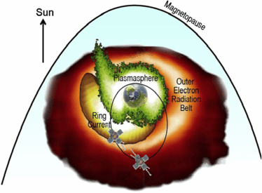

  

  A snapshot of the orbits of the 2 RBSP spacecraft in the context of structures within Earth’s inner magnetosphere

  Fig. 19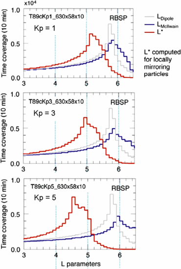

  

  Modeled, RBSP mission-summed sampling of uniform time samples (10 minutes) of various values of the radial magnetospheric L-parameter (in R _E ) for various magnetospheric dynamic conditions as characterized by the activity parameter Kp for inactive conditions (Kp=1), modestly active conditions (Kp=3) and relatively active conditions (Kp=5). The grey curve shows the Kp-independent result for sampling the McIlwain L-parameter in a purely dipole field, and the blue curves show the sampling of that same parameter for the Kp-dependent TS89 magnetic field model (Tsyganenko 1989). The red curve shows the sampling of the so-called L ^∗ parameter, which is the L-shall value of the purely dipolar magnetic field configuration that contains the same magnetic flux as would the particle drift orbit within the true distorted magnetic field configuration. L ^∗ is equivalent to the 3rd adiabatic invariant of particle motion. The McIlwain L-parameter and the L ^∗ parameter are defined, for example, by Roederer (1970); see Ukhorskiy and Sitnov (this issue). L ^∗ has become an increasingly important standard parameter for ordering radiation belt measurements (e.g. Fig. 10)

• (3) The lines of apogee for the two spacecraft precess in local time at a rate of about 210^∘ per year in the clockwise direction (looking down from the north). The 2 year nominal mission lifetime (∼4 years of expendables are available) allows all local times to be studied. By starting the mission with lines of apogee at dawn (a Program Level mission requirement), the nightside hemisphere will be accessed twice within the nominal 2 year mission lifetime.

• (4) Slightly different (∼130 km) orbital apogees cause one spacecraft to lap the other every ∼75 days, corresponding to about twice for every quadrant of the magnetosphere visited by the lines of apogee during the two year mission.

• (5) Because the spacecraft lap each other, their radial spacing varies periodically between ∼100 km and ∼5 R _E ; and resampling times for specific positions vary from minutes to 4.5 hours.

• (6) The orbital cadence (9 hour periods; an average of 4.5 hours between inbound and outbound sampling for each spacecraft) is faster than the relevant magnetic storm time scales (day).

• (7) The low inclination (10^∘) allows for the measurements of most of the magnetically trapped particles; while the precession of the line of apogee and the tilt of the Earth’s magnetic axis enables nominal sampling to magnetic latitudes of 0±21^∘ (Fig. 20).

  Fig. 20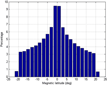

  

  RBSP mission-averaged sampling of magnetic latitude calculated using a tilted dipole magnetic field model

• (8) Spacecraft spin axes point roughly Sunward. Due to orbit precession, the spin axis must be re-aligned with respect to the sun periodically once each ∼21 days. The spin axis is always maintained to lie within 27^∘ of the sun’s direction.

• (9) The 5 RPM spin period of the spacecraft, the nominal sunward orientation of the spin axis, and the positioning of the spacecraft near the magnetic equator of the quasi-dipolar magnetic configuration, combine to enable the particle detectors to obtain fairly complete pitch angle distributions twice for every spin of the spacecraft and the electric field instrument to make excellent measurements of the crucial dawn/dusk electric field.

RBSP is expected to see perhaps 2 dozen magnetic storms during its nominal 2-year lifetime. During critical events (e.g. the several hours that comprise “main phase” periods of magnetic storms), the two spacecraft will perform radial cuts through the inner regions with separation times that vary from minutes to several hours. For each quadrant of Earth’s magnetosphere, perhaps 6 storms will be observed within the first 20 months, and again specific features will be sampled with a distribution of separation distances and times. In this way, a range of spatial and temporal scales will be examined by the RBSP mission. To the extent that features such as the “bump” displayed in Fig. 17 characterize radiation belt responses to storms and other processes, as we know they do (Fig. 10), the RBSP mission will definitively distinguish the spatial from temporal structures and establish how they are generated.

Members of the RBSP team will employ modeling and partnerships with other missions to infer details concerning some crucial processes. For example, some strong whistler mode interactions that may energize electrons can occur at relatively high magnetic latitudes, particularly on the dayside (Horne et al. 2005a, 2005b; Bortnik et al. 2008). In the absence of other assets, RBSP will infer the characteristics of such interactions by observing the low-latitude consequences of such interactions and combining those observations with the sophisticated models that are now being brought to bear on the problem (e.g. Bortnik et al. 2008). Additionally, although the RBSP instruments do not have the pitch angle resolution to measure particle fluxes within the atmospheric loss cone, such particles are precisely those that will be measured by the Mission of Opportunity BARREL mission, which focuses upon the radiation belt particles precipitating into the atmosphere (Millan et al. this issue). BARREL will launch a series of balloon-borne X-ray sensors from the Antarctic during two month-long phases of the RBSP mission. Sensors on the SAMPEX, DMSP, and POES spacecraft can also be used to address this particle population. Third, the RBSP team will work with other missions such as THEMIS and geosynchronous spacecraft capable of measuring source populations outside the 5.8 R _E apogee of the RBSP mission. Finally, ACE and other missions will supply information concerning the interplanetary drivers such as the interplanetary magnetic field, and prevailing solar wind conditions.

4.2 RBSP Observations and Instruments

The observation requirements for the RBSP mission and spacecraft payload are delineated in the Program Level (Level-1) requirements document. The verifiable requirements in that document are expressed in the form of specific parameter measurements (e.g. energy ranges, energy resolution, frequency ranges, time cadences, etc.). The “observations” from which these verifiable requirements are derived are in paragraphs that express the “intent” of the mission measurements. Those intended “observations” are paraphrased in the table provided here in Table 1. A survey of these intended observations and their purposes provides an appreciation for the comprehensive measurements provided by the RBSP payload.

Table 1 RBSP program level (Level-1) observations

The parameter measurement requirements for the RBSP payload, derived by putting the observational needs (Table 1) into the context of the characteristics of Earth’s inner and middle magnetosphere, are shown in the Level-1 document tables reproduced in Fig. 21. The instruments and instrument suites that will provide these measurements are summarized here in Table 2. This table also shows the PSBR Investigation, which includes the RPS instrument, a contributed, but not required, element that will fly as part of the RBSP payload on each spacecraft. It targets the inner proton belt by measuring proton energies up to 2 GeV. Additionally, the figure includes the BARREL Mission of Opportunity investigation (mentioned above) which involves balloon payloads flown in the Antarctic in conjunction with the RBSP mission. Each of the entries in Table 2 has one or more chapters in this special issue describing the details and capabilities of the instrumentation.

Fig. 21

RBSP measurement parameter requirements as specified in the RBSP Program Level requirements document. These measurement requirements are derived from the observation needs summarized in Table 1

Table 2 RBSP investigations

The particle energy and species coverage requirements versus payload capabilities are shown graphically in Fig. 22. Similarly, the electric and magnetic fields frequency range requirements versus payload capabilities are shown in Fig. 23. These graphical displays demonstrate the comprehensive and coordinated nature of the RBSP payload elements. As an additional requirement within the Program Level requirements document, the “fields” payload elements must be capable of taking concurrent full 3 dimensional (3D) magnetic and 3D electric waveforms with at least 20 k samples/s to determine the propagation characteristics of waves up to 10 kHz. This capability is implemented as a burst capability within the EFW and EMFISIS instruments (Table 2; see Wygant et al. this issue, and Kletzing et al. this issue). What is not apparent from Fig. 22 regarding the particle measurement is the fact that, because of the use of multi-parameter sensing techniques for both electrons and ions, the RBSP particle measurements will be, as a set, the cleanest measurements yet taken in this harsh environment relative to the contamination from penetration radiation (Baker et al. this issue; Blake et al. this issue; Funsten et al. this issue; Lanzerotti et al. this issue; Mazur et al. this issue).

Fig. 22

Comparison between the RBSP particle measurement requirements and instrument capabilities for the range of energies and species to be measured

Fig. 23

Comparison between the RBSP fields measurement requirements and instrument capabilities for the range of frequencies and fields types to be measured

5 Closing Remarks

The high level objectives of the RBSP mission are articulated in Sect. 1. To achieve those objectives it is necessary to develop science questions, like those presented in Sect. 2, that are specific enough to invite the generation of testable hypotheses. The RBSP mission design has many of the capabilities that are needed to discriminate between and test these hypotheses. Most critical is the ability of RBSP to perform simultaneous multipoint sampling over a broad spectrum of spatial and temporal scales, combined with extremely capable and highly coordinated instrumentation. These capabilities will enable researchers to discriminate between time and space variations. With such capabilities one may compare the time scales for the generation of local particle acceleration features with the theoretical expectations based on the measurements of the static and dynamic fields. With such capabilities one may measure rather than just infer the gradients that generate currents and the gradients that reveal electric potential distributions. With the capabilities of the RBSP instrumentation, one may determine the detailed characteristics of resonant interactions between particle and waves.

An important element in achieving complete science closure for some of the science objectives is the utilization of sophisticated models and simulations to place the RBSP multipoint measurements into the broader 3-dimensional picture. Strong coordination between data analysts and model builders is described in each of the investigation reports in this special issue, and specifically in the articles by Spence et al., Kletzing et al., Lanzerotti et al., Wygant et al., and Ginet et al.

A distinction is made in the structure of this special issue on the RBSP mission between the instrument investigations and the instruments themselves. The papers cited at the end of the last paragraph describe the instrument investigation for the ECT, EMFISIS, RBSPICE, EFW, and PSBR investigations (see Table 2). These papers describe in various degrees the science objectives of the individual team investigations, the science teams involved, the data processing, analysis, and archiving plans, the role of theory and modeling in resolving the targeted science issues, and the role of modeling in synthesizing the limited two point measurements that are made by the RBSP instruments. The instrumentation associated with these instrument investigations are in some cases described within the same instrument investigation papers (EMFISIS: Kletzing et al.; RBSPICE: Lanzerotti et al.; and EFW: Wygant et al.). In other cases the instrumentation is described in separate papers (ECT-HOPE: Funsten et al.; ECT-MagEIS: Blake et al.; ECT-REPT: Baker et al.; PSBR-RPS: Mazur et al.; again see Table 2).

Other papers in this special issue describe engineering details of the RBSP mission (Stratton et al.), the RBSP spacecraft (Kirby et al.), the RBSP contributions to the practical issues of space weather (Kessel et al.), the overarching RBSP data processing, analysis, dissemination, and archiving plans (Science Operations: Fox et al.), and the RBSP Education and Public Outreach plan (EPO: Fox et al.). Additionally, Ukhorskiy and Sitnov review present understanding regarding the definitions and calculations of various parameters that order the radiation belts and the mathematical tools that are used to manipulate those parameters; and Millan et al. describe the Mission of Opportunity Antarctic high-altitude balloon program called BARREL that will make measurements of precipitated electrons in coordination with the RBSP mission. Finally, Goldsten et al. describe an engineering sub-system, the Environmental Radiation Monitor that measures total radiation dose under various shielding thickness and monitors the potential for deep dielectric discharge by measuring the penetrating electron current delivered to two deeply buried conductors.

References

D.N. Baker, R.D. Belian, P.R. Higbie, E.W. Hones Jr., J. Geophys. Res. 84(A12), 7138–7154 (1979). doi:10.1029/JA084iA12p07138
D.N. Baker, E.W. Hones Jr., P.R. Higbie, R.D. Belian, P. Stauning, J. Geophys. Res. 86(A11), 8941–8956 (1981). doi:10.1029/JA086iA11p08941
D.N. Baker, S.G. Kanekal, X. Li, S.P. Monk, J. Goldstein, J.L. Burch, Nature 432, 878 (2004). doi:10.1038/nature03116
D.N. Baker et al., The relativistic electron-proton telescope (REPT/ECT) instrument on board the radiation belt storm probes (RBSP) spacecraft: characterization of Earth’s radiation belt high-energy particle populations, this issue
J.B. Blake, W.A. Kolasinski, R.W. Fillius, E.G. Mullen, Geophys. Res. Lett. 19(8), 821–824 (1992). doi:10.1029/92GL00624
J.B. Blake et al., The MagEIS/ECT instrument on the RBSP mission, this issue
J. Bortnik, R.M. Thorne, U.S. Inan, Geophys. Res. Lett. 35, L21102 (2008). doi:10.1029/2008GL035500
W.J. Burke, L.C. Gentile, C.Y. Huang, J. Geophys. Res. 112, A07208 (2007). doi:10.1029/2006JA012137
C. Cattell et al., Geophys. Res. Lett. 35, L01105 (2008). doi:10.1029/2007GL032009
Y. Chen, G.D. Reeves, R.H.W. Friedel, Nature Physics, 1 July 2007. doi:10.1038/nphys655
S.P. Christon, D.J. Williams, D.G. Mitchell, C.Y. Huang, L.A. Frank, J. Geophys. Res. 96(A1), 1–22 (1991). doi:10.1029/90JA01633
A.J. Dessler, E.N. Parker, Hydromagnetic theory of geomagnetic storms. J. Geophys. Res. 64(12), 2239–2252 (1959). doi:10.1029/JZ064i012p02239
W.C. Feldman, J.R. Asbridge, S.J. Bame, M.D. Montgomery, S.P. Gary, J. Geophys. Res. 80(31), 4181–4196 (1975). doi:10.1029/JA080i031p04181
M.-C. Fok, T.E. Moore, W.N. Spjeldvik, J. Geophys. Res. 106, 3873–3881 (2001a). doi:10.1029/2000JA000150
M.-C. Fok, R.A. Wolf, R.W. Spiro, T.E. Moore, J. Geophys. Res. 106, 8417–8424 (2001b). doi:10.1029/2000JA000235
N.J. Fox, B.H. Mauk, J.B. Blake, Geophys. Res. Lett. 33, L18108 (2006). doi:10.1029/2006GL026598
N.J. Fox, M. Weiss, R. Barnes, The RBSP science operations plans, this issue
H.O. Funsten et al., The HOPE/ECT instrument on the RBSP mission, this issue
G.P. Ginet et al., AE9/AP9/SPM: models for specifying the trapped energetic particle and space plasma environment, this issue
J.O. Goldsten, R.E.H. Maureer, P.N. Peplowski, A. Holmes-Siedle, C.C. Herrmann, B.H. Mauk, The RBSP engineering radiation monitor, this issue: doi:10.1007/s11214-012-9917-x
J.C. Green, M.G. Kivelson, J. Geophys. Res. 109, A03213 (2004). doi:10.1029/2003JA010153
W.N. Hess, The Radiation Belt and Magnetosphere (Blaisdell, Boston, 1968)
T. Hori, A.T.Y. Lui, S. Ohtani, P. Cson Brandt, B.H. Mauk, R.W. McEntire, K. Maezawa, T. Mukai, Y. Kasaba, H. Hayakawa, J. Geophys. Res. 110, A04213 (2005). doi:10.1029/2004JA010449
R.B. Horne, R.M. Thorne, Geophys. Res. Lett. 25(15), 3011–3014 (1998). doi:10.1029/98GL01002
R.B. Horne, R.M. Throne, N.P. Meredith, R.R. Anderson, J. Geophys. Res. 108(A7), 1290 (2003). doi:10.1029/2002JA009736
R.B. Horne et al., Nature 437, 227–230 (2005a). doi:10.1038/nature03939
R.B. Horne, R.M. Thorne, S.A. Glauert, J.M. Albert, N.P. Meredith, R.R. Anderson, J. Geophys. Res. 110, A03225 (2005b). doi:10.1029/2004JA010811
R.B. Horne, R.M. Thorne, S.A. Glauert, N.P. Meredith, D. Pokhotelov, O. Santolík, Geophys. Res. Lett. 34, L17107 (2007). doi:10.1029/2007GL030267
M.K. Hudson, G.T. Kress, H.-R. Mueller, J.A. Zastrow, J.B. Blake, J. Atmos. Sol.-Terr. Phys. 70, 708–729 (2008)
R.H.A. Iles, N.P. Meredith, A.N. Fazakerley, R.B. Horne, J. Geophys. Res. 111, A03204 (2006). doi:10.1029/2005JA011206
A.S. Jursa, Handbook of Geophysics and the Space Environment (Air Force Geophysics Laboratory, Hanscom, 1985)
P.J. Kellogg, C.A. Cattell, K. Goetz, S.J. Monson, L.B. Wilson III, Geophys. Res. Lett. 37, L20106 (2010). doi:10.1029/2010GL044845
K. Kersten, C.A. Cattell, A. Breneman, K. Goetz, P.J. Kellogg, J.R. Wygant, L.B. Wilson III, J.B. Blake, M.D. Looper, I. Roth, Geophys. Res. Lett. 38, L08107 (2011). doi:10.1029/2011GL046810
R.L. Kessel, N.J. Fox, M. Weiss, RBSP and space weather, this issue
G.V. Khazanov, K.V. Gamayunov, V.K. Jordanova, J. Geophys. Res. 108(A12), 1419 (2003). doi:10.1029/2003JA009856
K.W. Kirby et al., Radiation belt storm probe spacecraft and environments, this issue
M.G. Kivelson, C.T. Russell, Introduction to Space Physics (Cambridge University Press, Cambridge, 1995)
C. Kletzing et al., The electric and magnetic field instrument suite and integrated science (EMFISIS) on RBSP, this issue
L.J. Lanzerotti et al., Radiation belt storm probes ion composition experiment (RBSPICE), this issue
J.F. Lemaire, D. Heynderickx, D.N. Baker, Radiation Belts, Models and Standards, Geophysical Monograph, vol. 97 (American Geophysical Union, Washington, 1996)
X. Li, I. Roth, M. Temerin, J.R. Wygant, M.K. Hudson, J.B. Blake, Geophys. Res. Lett. 20(22), 2423–2426 (1993). doi:10.1029/93GL02701
L.Y. Li, J.B. Cao, G.C. Zhou, X. Li, J. Geophys. Res. 114, A12214 (2009). doi:10.1029/2009JA014333
X. Li, M. Temerin, D.N. Baker, G.D. Reeves, J. Geophys. Res. 116, A11207 (2011). doi:10.1029/2011JA016934
M.W. Liemohn, J. Geophys. Res. 108(A6), 1251 (2003). doi:10.1029/2003JA009839
R.P. Lin, Space Sci. Rev. 86, 61–78 (1998)
K.R. Lorentzen, M.D. Looper, J.B. Blake, Relativistic electron microbursts during the GEM storms. Geophys. Res. Lett. 28(13), 2573–2576 (2001). doi:10.1029/2001GL012926
G.H. Ludwig, Opening Space Research, Dreams, Technology, and Scientific Discovery (Geopress, American Geophysical Union, Washington, 2011)
A.T.Y. Lui, R.W. McEntire, S.M. Krimigis, E.P. Keath, in Ion Acceleration in the Magnetosphere and Ionosphere. Geophysical Monograph, vol. 38 (American Geophysical Union, Washington, 1986), pp. 149–152
G.M. Mason, D.N. Baker, J.B. Blake, L.B. Callis, D.C. Hamilton, D. Hovestadt, B. Klecker, R.A. Mewaldt, M. Scholer, E.C. Stone, T.T. von Rosenvinge, SAMPEX mission overview, in Particle Astrophysics: the NASA Cosmic Ray Program for the 1990s and Beyond. AIP Conference Proceedings, vol. 203 (American Institute of Physics, New York, 1990), pp. 44–47
B.H. Mauk, N.J. Fox, J. Geophys. Res. 115, A12220 (2010). doi:10.1029/2010JA015660
J. Mazur et al., The relativistic proton spectrometer (RPS) sensor for the radiation belt storm probes mission, this issue
C.E. McIlwain, J. Geophys. Res. 66(11), 3681–3691 (1961). doi:10.1029/JZ066i011p03681
N.P. Meredith, R.B. Horne, R.H.A. Iles, R.M. Thorne, D. Heynderickx, R.R. Anderson, J. Geophys. Res. 107(A7), 1144 (2002). doi:10.1029/2001JA900146
N.P. Meredith, M. Cain, R.B. Horne, R.M. Thorne, D. Summers, R.R. Anderson, J. Geophys. Res. 108(A6), 1248 (2003). doi:10.1029/2002JA009764
R.M. Millan, K.B. Yando, J.C. Green, A.Y. Ukhorskiy, Geophys. Res. Lett. 37, L20103 (2010). doi:10.1029/2010GL044919
R. Millan et al., The BARREL mission of opportunity investigation for the RBSP mission, this issue
R. Nakamura, M. Isowa, Y. Kamide, D.N. Baker, J.B. Blake, M. Looper, J. Geophys. Res. 105(A7), 15,875–15,885 (2000). doi:10.1029/2000JA900018
T.P. O’Brien, M.D. Looper, J.B. Blake, Geophys. Res. Lett. 31, L04802 (2004). doi:10.1029/2003GL018621
G.D. Reeves, K.L. McAdams, R.H.W. Friedel, T.P. O’Brien, Geophys. Res. Lett. 30(10), 1529 (2003). doi:10.1029/2002GL016513
J.G. Roederer, Dynamics of Geomagnetically Trapped Radiation (Springer, Berlin, 1970)
D.E. Rowland, J.R. Wygant, J. Geophys. Res. 103(A7), 14,959–14,964 (1998). doi:10.1029/97JA03524
D.M. Sawyer, J.I. Vette, AP-8 trapped proton environment for solar maximum and solar minimum, NSSDC/WDC-A-R&S 76-06, NASA-GSFC TMS-72605 (1976)
M. Schulz, L.J. Lanzerotti, Particle Diffusion in the Radiation Belts (Springer, Berlin, 1974)
N. Sckopke, J. Geophys. Res. 71, 13 (1966). doi:10.1029/JZ071i013p03125
G.W. Singley, J.I. Vette, The AE-4 model of the outer radiation zone electron environment, NSSDC 72-06 (1972)
H.E. Spence et al., The ECT investigation on the RBSP mission, this issue
J.M. Stratton, R.J. Harvey, G.A. Heyler, Mission overview for the radiation belt storm probes mission, this issue: doi:10.1007/s11214-012-9933-x
Z. Su, F. Xiao, H. Zheng, S. Wang, Geophys. Res. Lett. 38, L06106 (2011). doi:10.1029/2011GL046873
D. Summers, R.M. Thorne, F. Xiao, J. Geophys. Res. 103(A9), 20,487–20,500 (1998). doi:10.1029/98JA01740
R.M. Thorne, Geophys. Res. Lett. 37, L22107 (2010). doi:10.1029/2010GL044990
R.M. Thorne, T.P. O’Brien, Y.Y. Shprits, D. Summers, R.B. Horne, J. Geophys. Res. 110, A09202 (2005). doi:10.1029/2004JA010882
N.A. Tsyganenko, A magnetospheric magnetic field model with a warped tail current sheet. Planet. Space Sci. 37, 5 (1989)
D.L. Turner, Y. Shprits, M. Hartinger, V. Angelopoulos, Nature Phys. 8, 208 (2012). doi:10.1038/NPhysics2185
E.D. Turney, A.M. Novak, K. Beisser, N. Fox, Radiation belt storm probes (RBSP) education and public outreach program, this issue
A.Y. Ukhorskiy, M. Sitnov, Dynamics of radiation belt particles, this issue
A.Y. Ukhorskiy, B.J. Anderson, P.C. Brandt, N.A. Tsyganenko, J. Geophys. Res. 111, A11S03 (2006)
A. Ukhorskiy, P. O’Brien, D. Sibeck, Special issue: dynamic variability of Earth’s radiation belts. J. Atmos. Sol.-Terr. Phys. 70(14), 1679–1846 (2008)
J.A. Van Allen, Origins of Magnetospheric Physics (Smithsonian Inst., Washington, 1983)
M. Walt, in Discovery of the Magnetosphere, ed. by C.S. Gillmaor, J.R. Spreiter. History of Geophysics, vol. 7 (American Geophysical Union, Washington, 1997), pp. 253–264
J.R. Wygant et al., The EFW investigation and instruments on the RBSP mission, this issue
I.V. Zavidonov, Sputniks, explorers, and propaganda: the discovery of the Earth’s radiation belts. Hist. Technol. 17, 99–124 (2000)
Acknowledgements
We very much appreciate the efforts of Thomas Sotirelis, Kazue Takahashi, and Gene Heyler in generating several of the important plots and analyses for this paper, most specifically, Figs. 19 and 20.
Open Access
This article is distributed under the terms of the Creative Commons Attribution License which permits any use, distribution, and reproduction in any medium, provided the original author(s) and the source are credited.
Author information
Authors and Affiliations
Corresponding author
Rights and permissions
Open Access This article is distributed under the terms of the Creative Commons Attribution 2.0 International License (https://creativecommons.org/licenses/by/2.0), which permits unrestricted use, distribution, and reproduction in any medium, provided the original work is properly cited.
About this article
Cite this article
Mauk, B.H., Fox, N.J., Kanekal, S.G. et al. Science Objectives and Rationale for the Radiation Belt Storm Probes Mission. Space Sci Rev 179, 3–27 (2013). https://doi.org/10.1007/s11214-012-9908-y
Received:
Accepted:
Published:
Issue Date:
DOI: https://doi.org/10.1007/s11214-012-9908-y