The Neutral Mass Spectrometer on the Lunar Atmosphere and Dust Environment Explorer Mission

Abstract

The Neutral Mass Spectrometer (NMS) of the Lunar Atmosphere and Dust Environment Explorer (LADEE) Mission is designed to measure the composition and variability of the tenuous lunar atmosphere. The NMS complements two other instruments on the LADEE spacecraft designed to secure spectroscopic measurements of lunar composition and in situ measurement of lunar dust over the course of a 100-day mission in order to sample multiple lunation periods. The NMS utilizes a dual ion source designed to measure both surface reactive and inert species and a quadrupole analyzer. The NMS is expected to secure time resolved measurements of helium and argon and determine abundance or upper limits for many other species either sputtered or thermally evolved from the lunar surface.

1 Scientific Objectives of the LADEE NMS

1.1 Lunar Atmosphere

The atmosphere of the moon is so tenuous that collisional interactions between free particles are entirely negligible. Each atom travels through the atmosphere in a ballistic trajectory that begins and usually ends on the lunar surface. The exceptions are particles that are ionized by solar photons, and those that leave the surface with speeds greater than the escape speed, which is nominally 2.38 km s⁻¹ but vary with the acceleration due to radiation pressure, and with the proximity of the trajectory to the L1 or L2 Lagrangian equilibrium point.

As envisioned pre-Apollo by Hodges and Johnson (1968), there are 2 categories of atoms, those that “condense” on the cold nighttime surface of the moon, and those that do not. Gases that condense at night ride on the rotating lunar surface, as on a conveyor belt, and evaporate as the surface temperature increases following sunrise, forming a pocket of gas over the sunrise terminator. Those that do not condense tend to obey the law of exospheric equilibrium (1), which to first order is

$$ n T^{5/2} \approx \mathrm{constant} $$

(1)

where n is surface concentration and T is temperature.

With the knowledge gained from Apollo returned samples, the theory of the surface interaction process has evolved into something more complicated than condensation and evaporation. Upon striking the lunar surface, an atom finds itself in a fairy-castle-like structure of loosely packed, micron-scale grains, wherein the grain surface area is several thousands of cm² per gram. The statistics of inter-grain vertical transport is similar to a 1-dimensional random walk, that is, the mean number of encounters is about 2, but the average is infinite (Hodges 1980). Each encounter with a grain can end in 2 ways. One is elastic scattering through phonon transfer. The other is thermal accommodation, a 2-step process of adsorption, followed by desorption with a residence time determined by the temperature dependence of the Arrhenius equation. The adsorption/desorption process is analogous to condensation/evaporation in the sense that vapor pressure is derived from the former.

Elastic scatter tends to create a Maxwellian distribution of velocities, while desorbing atoms have a higher energy Knudsen (or Maxwell-Boltzman-flux) distribution. The result of multiple grain encounters is a hybrid velocity distribution and a non-barometric altitude profile.

1.2 Ground Truth

The Apollo 17 mass spectrometer established the presence of helium and argon-40 in the nighttime lunar atmosphere. Owing to operational constraints, there are no daytime data.

Black curves in Fig. 1 show the nighttime part of the diurnal variation helium at the Apollo 17 site during the first 10 lunations of 1973 (Hodges and Hoffman 1974). Overlays in red are Monte Carlo simulations derived with the aid of the LExS (Lunar Atmosphere Simulation) tool kit (Hodges 2011). On average, the nighttime maximum of helium approximates the T ^5/2 law of exospheric equilibrium. Fluctuations of the black curves with respect to the red ones reflect variations in one of the sources of helium, which are solar wind α-particles and radiogenic He escaping from the lunar interior.

Fig. 1

Helium data from the Apollo 17 mass spectrometer (black) and simulated data (red). Day of year 1973 is annotated on abscissa

The presence of ⁴⁰Ar in the lunar atmosphere was foretold by Apollo 11 soils that had apparent K/Ar ages that are older than the solar system. Yaniv et al. (1972) gave a prescient explanation of the parentless argon as re-trapped atmospheric ions. In other words, the atmosphere of the moon includes argon that is supplied by radiogenesis in the interior of the moon.

Thus it was not surprising that ⁴⁰Ar was detected by the Apollo 17 mass spectrometer. However, the diurnal behavior shown for 2 lunations in Fig. 2 (Hodges and Hoffman 1974) was unexpected. In the distinctly non-equilibrium nighttime pattern, the post-sunset decay of argon is easily associated with adsorption as the surface cools, and the pre-sunrise build-up suggests rapid desorption at sunrise. This is essentially the prediction of Hodges and Johnson (1968) for a condensable gas, like water vapor. For argon, this behavior requires pristine grain surfaces that have not been exposed to enough water vapor to form a monolayer (Hodges 2001).

Fig. 2

Apollo 17 measurements of ⁴⁰Ar from 2 lunations of 1973

A second noteworthy feature of Fig. 2 is the difference in the amplitudes of the diurnal profiles, which implies that during the March to July interval, escape exceeded supply, creating a noticeable decrease in the total abundance of argon on the moon. What is clear is that the release of radiogenic gases from the interior of the moon is episodic; the Apollo 17 data suggest a correlation with tele-seismic events. It follows that argon may disappear from the lunar atmosphere during prolonged periods of low seismic activity.

1.3 Expectations of the LADEE NMS

Simulations of expected NMS orbital data, constructed with the aid of LExS and using instrument sensitivities described in this manuscript, are shown in Fig. 3 for orbits with periapses at sunrise. In addition to helium and argon whose densities are predicted from previous observations (e.g. Hodges et al. 1974; Stern 1999), the graph includes several species that might be supplied by thermalized solar wind. Since these species have not been observed, these simulations are included primarily to illustrate the LExS predictions of their variation along a typical LADEE orbit. The abscissa is time from periapsis and the sunrise terminator. The scale of ordinates, counts per second, is chosen to emphasize the degree of statistical uncertainty in the expected data if these species are detected and the vulnerability of the data to the background artifacts. Oxygen is presumed to combine on internal NMS surfaces to form O₂ although the actual behavior of atomic oxygen in the closed source in this low density environment cannot be predicted from the available data.

Fig. 3

Simulated LADEE NMS data for 3 orbits with periapsis at sunrise. Bold lines cover power-limited measurement periods; light extensions what would be measured if additional power were available

Wide segments of the curves of Fig. 3 cover periods of operation of the NMS, while thin line extensions are what could be expected if sufficient power were available to operate throughout an orbit.

1.4 Reduction of Orbital Data

To make sense of the orbital data it is necessary to project concentrations measured at various satellite altitudes to a reference level, the logical candidate being the USGS reference geoid radius of r ₀=1737.4 km. This projection will be derived from the altitude profile

$$ \ln \frac{n}{n_{0}} = \sum_{i} A_{i} \bigl\{ ( r/ r_{0} )^{i} -1\bigr\} $$

(2)

where the i=1 term is hydrostatic equilibrium that would arise if all atoms were to accommodate and leave the surface with a Knudsen distribution of velocities. Higher order terms are needed to account for the Maxwellian component as well as the mix of gas temperatures in the down-coming fraction due to lateral gradients of surface temperature (Hodges 1972).

Figure 4 illustrates the differences between altitude profiles for hydrostatic equilibrium (dashed lines) and LExS simulations that account for lateral flow and the un-accommodated fraction of atoms leaving the surface. Note that at high altitudes the slope of the simulated dayside profile for sunrise +2° approaches the slope of hydrostatic equilibrium. However, just 2° on the night side of the sunrise terminator, where upward going atoms are cold while the day to night flux is relatively hot, the latter obviously dominates at high altitude.

Fig. 4

Simulated vertical profiles of ⁴⁰Ar at noon and sunrise at +2^∘ longitude. Dashed lines are classical hydrostatic equilibrium profiles included to elucidate non-thermal properties

A fortuitous aspect of the LADEE mission is that frequent orbit maintenance maneuvers are required to keep periapsis above the surface. Contamination modeling demonstrated that the flux of gas from the LADEE thrusters located well away from the NMS during these maneuvers into the NMS would be negligible. NMS measurements of ambient gas concentrations collected immediately before and after each OMM will provide local scale heights over a substantial range of altitudes. At the end of the mission, the OMM data set will be used to create normalized altitude profiles that, in turn, will facilitate the reduction of orbital data to the geoid radius. In addition, these data will be invaluable in the synthesis of accommodation coefficients and energies of activation in the lunar regolith

1.5 The LADEE Mission Duration and Orbit

The LADEE spacecraft bus is a modular design utilizing a carbon composite structure that could be adapted for use with a variety of launch vehicles. In this case the spacecraft with its three instruments and a laser communications technology demonstration unit are adapted to a Minotour V launch vehicle launched from the Wallops Flight Facility for a nominal 100 day science mission after a commissioning period of 30 days. The commissioning phase in a lunar elliptical orbit of approximately 250—275 km also allows the tests of the optical communications module. For the science orbit an elliptical orbit will also be utilized to conserve propulsion but with periapsis to 50 km and below and an orbital time of typically less than 2 hours. With limited battery capacity the measurement time during orbits will typically be shared between the NMS, the Lunar Dust Experiment (LDEX), and the Ultraviolet and Visible Light Spectrometer (UVS) but not operating all three instruments concurrently.

2 Instrument Description

2.1 Introduction and Heritage

Many elements of the Neutral Mass Spectrometer have a heritage in mass spectrometers previously developed for planetary or Earth orbiting satellites. The quadrupole mass analyzer and detector systems are similar to those developed for Venus (Niemann et al. 1980), the upper atmosphere of Mars (Niemann et al. 1998), the deep atmosphere of Jupiter (Niemann et al. 1992), and the atmosphere of Titan (Niemann et al. 1997). In all of these experiments the gas sampling and pumping systems, if required, were specifically designed for the target environments. Direct heritage for the NMS design came from the Ion and Neutral Mass Spectrometer (INMS) on the Cassini Orbiter (Kasprzak et al. 1996) and the Comet Nucleus Tour (CONTOUR) (Veverka et al. 1995) Neutral Gas and Ion Mass Spectrometer (CONTOUR-NGIMS) which were modifications of the NGIMS instrument design for the Comet Rendezvous Flyby Mission (CRAF) that was under development when that mission was canceled. In fact, the approach taken for the LADEE-NMS was to utilize the engineering unit sensor from the CONTOUR-NGIMS and to develop a new set of electronics. The CONTOUR NGIMS and the Cassini INMS (Kasprzak et al. 1996; Waite et al. 2004) experiments utilized an electrostatic 90 degrees deflector (Mahaffy 1990) designed to multiplex two separate ion sources to the quadrupole analyzer (Fig. 5).

Fig. 5

A schematic view of the gas and ion path in the NMS

Significant improvements to the INMS design, however, were implemented in both the CONTOUR-NGIMS and the NMS designs to optimize the measurement for sensitivity. In order to allow the measurement of trace species in the short integration time available in a comet nucleus flyby and in the low-density exosphere of the moon, the sensitivity of the CONTOUR-NGIMS and the LADEE-NMS were extended considerably beyond that of any mass spectrometer previously developed for planetary applications with nominal sensitivity for ⁴⁰Ar of 2.3×10⁻² (counts/sec)/(part/cc). In addition, the CONTOUR NGIMS was designed with mass dependent adjustment of the quadrupole bias and electrode focusing voltages for the considerably higher comet nucleus flyby velocities in the cometary coma nuclei encounters compared to the Cassini Orbiter flyby velocity at Titan. Each of the heritage mass spectrometers could operate at unit mass resolution over the full spectral range (2–99 Da in the case of the Cassini-INMS and 2–294 Da in the case of the CONTOUR-NGIMS). Figures 6, 7, and 8 respectively show the NMS instrument during and after integration, the ion source and mass analyzer, and the sensor housing and detector assembly.

Fig. 6

The left panel shows the main electronics box (MEB), the break off cap (BOC), the vacuum housing (VH), the radio frequency (RF) electronics, and the detector (Det) electronics. In the right panel view the covers and red tag items are also shown as is the ion source cover (ISC)

Fig. 7

The ion source assembly is shown on the top left with the open source (OS), closed source (CS), and quadrupole deflector (QD). The quadrupole rod assembly is shown on the right

Fig. 8

The mass spectrometer housing is shown in the left panel and the detector assembly on the right. The outside diameter of the detector housing is 5.08 cm. The larger pins on the welded electrical feedthrough assembly are for the RF voltages applied to the quadrupole rods. The pinch-off tube is seen to the left of the feedthrough assembly. The dual detector assembly show at right is mounted on a flange that utilizes a gold plated Inconel “c” seal to achieve ultra-high-vacuum. The NMS specifications are shown in Table 1

The mass spectrometer schematic (Fig. 5) shows the sensor including the ion source assembly with the quadrupole deflector for multiplexing ions from the two sources into the mass analyzer, the sensor housing, the quadrupole rod assembly, and the dual detector system. Several of the instrument performance specifications are given in Table 1. The block diagram (Fig. 9) shows the various electronic subsystems.

Fig. 9

The NMS electrical block diagram

Table 1 NMS specifications

2.2 Neutral Gas and Ion Sampling

Closed Ion Source

The classic design of a closed ion source (Spencer and Carignan 1988) for upper atmosphere space research consists of a small aperture in a spherical antechamber. Gas flows into the source through this aperture and most of the gas eventually leaves through the same aperture after thermalization with the walls of the source.

A portion of the gas leaks out through a relatively small ion exit aperture, and another small portion is ionized and accelerated out of the source through the electrostatic deflector and into the entrance lens focusing system of the mass analyzer. The vent orthogonal to the open source axis that was included in the Cassini INMS design was closed in the NMS design to better quantify the relationship of the density in the ionization region to the ambient density. In the NMS design the entire sensor volume acts as a closed source. The density in a closed source of this geometry for species i can be shown (Wurz et al. 2007) from the relevant gas kinetic equations to be:

$$\begin{aligned} &n_{s,i} = n_{a,i} (T_{a,i}/T_{s,i})^{1/2} \bigl(\exp\bigl(-S_{i}^{2}\bigr) + \pi^{1/2} S_{i}\bigl[1 + \operatorname{erf}(S_{i})\bigr]\bigr) \\ &\quad\mbox{with}\ S_{i} = V \cos (\alpha)/c_{i} \ \mbox{and}\ c_{i} = (2kT_{a,i}/m_{i})^{1/2} \end{aligned}$$

where n= density and T=temperature, with the subscripts a and s designating the ambient and source values respectively for species i. V is the apparent bulk speed of the atmosphere in the spacecraft reference frame, α= the angle between the normal to the orifice and the spacecraft velocity vector, c _i = the most probable speed of the ambient gas particles, and k= Boltzmann’s constant. The classic closed source configuration will typically accept gas from nearly a 2π steradian field of view and will provide nearly a 50 % measurement duty cycle on a spinning spacecraft. The LADEE spacecraft is 3-axis stabilized during the NMS measurement periods.

Open Ion Source

The open ion source is designed to measure or lower the upper limit on species such as OH with a high upper limit of ∼1×10⁷ particles/cc that would be destroyed or transformed by collisions in the closed ion source. The NMS can also search for metal atoms or their oxides with this source.

In the open ion source, collimating apertures form a neutral beam of particles that pass through a crossed electron beam generated by focusing electrons emitted from a hot, 97 % tungsten, 3 % rhenium, 0.005″, 6-coil filament. A fraction of these particles are ionized and transported through the electrostatic deflector to the quadrupole analyzer. Ambient ions are swept out of the inlet path by a set of deflection electrodes before they reach the ionization region.

The electrostatic deflector is an energy dispersive device. The kinetic energy (0.5mv ²) of a neutral exospheric gas particle with mass m and velocity v in the spacecraft frame of reference is established by the spacecraft velocity combined with the velocity of the lunar particle determined by where it is on its ballistic trajectory after release from the lunar surface. The bandpass of the deflector is approximately 25 eV with the voltages selected for the NMS operation. The bias on the grid at the exit to the ionization region is set slightly positive to discriminate against the gas that has thermalized in the mass spectrometer. The efficiency of the open source is expected to be similar to that of the closed source with an identical electron gun design, but the exact relationship of the sensitivity of the two sources will only be established in space by comparison of the signals from a relatively abundant gas such as He or Ar from the open and closed sources since the voltage settings for nominal open source operation in lunar orbit are optimized through simulations to discriminate against open source thermalized gas and cannot be further verified in the laboratory without an atomic beam source.

2.3 Quadrupole Mass Analyzer and Detector

Quadrupole Mass Filter

The mass analyzer consists of four quadrupole rods precisely fabricated and assembled into a rigid parallel assembly to which a combination of radio frequency (RF) and static (DC) voltages are applied to achieve mass separation. The voltages (V _dc +V _ac cos(ωt)) and −(V _dc +V _ac cos(ωt)), where ω is the frequency of V _ac , are applied to opposite rod pairs resulting in a two-dimensional quadrupole field of the form

$$\phi (x, y) = \bigl(V_{dc} + V_{ac} \cos(\omega t) \bigr) \bigl(x^{2} - y^{2}\bigr)/R_{o}^{2} $$

where R _o is the distance from the z (symmetry) axis to the nearest rod surface, and x and y are the axes crossing both the z axis and nearest point of the adjacent rods. Two fixed frequencies were used over the 2–150 Da mass range of NMS: 3.0 MHz for the mass range 2 to 20.5 Da and 1.4 MHz for the range 20.5 to 150.5 Da. Small amplitude changes in the RF are made under software control to compensate for any temperature or frequency drifts. These corrections keep the analyzer tuning essentially constant over the instrument operating temperature range of −20 ^∘C to +40 ^∘C.

The V _dc has an additional bias voltage, V _bias , added to it that is a function of the mass. This voltage is adjusted during tuning to allow ions to spend sufficient time (cycles) in the mass resolving RF field thus reducing the mass peak width and hence increasing the mass resolution.

Detector Assembly

The NMS detector assembly consists of a system of ion focusing lenses and two redundant off-axis continuous channel electron multipliers. The ion focusing lens system consists of four lenses positioned between the exit of the quadrupole analyzer and the entrance of the multipliers. A voltage ranging from −200 V to 550 V is applied to each lens to focus the ions exiting the analyzer into the detectors.

The model 4870-channeltron electron multipliers were purchased from Photonis and were assembled in house. Finite element analysis was employed in the design of the detector housing to insure that these glass devices would not be damaged during the considerable vibrations incurred during the LADEE launch and the subsequent solid rocket motor burn. The NMS multipliers begin to saturate at several million counts per second with an average gain of 6×10⁷, and a background noise level of ∼8 counts per minute. The operating voltage is between −2400 V and −3000 V. The multipliers are positioned off axis of the quadrupole to avoid detecting spurious photons and neutrals. The two multipliers are assembled facing each other within their housing, providing a redundant system.

2.4 Electrical Design

Spacecraft Interface

The NMS Main Power is supplied via a single-string, spacecraft-switched, 5 A resettable circuit breaker operating at the nominal spacecraft bus voltage of 28 VDC with an operating range of 24 VDC to 34 VDC (Fig. 9). NMS Heater Power is also supplied by the spacecraft power bus via single-string, spacecraft-switched, 1A resettable circuit breakers. One switch is dedicated to the Bakeout Heater and two switches are dedicated to the Main Electronics Box (MEB) and RF Survival Heaters. Any, or all, buses may be turned on in any order and the maximum possible power from all busses is approximately 45 W. Power usage during experiment operation is a function of the commanded instrument mode with the power sequencing on 30 ms intervals.

The spacecraft also provides four switches for commanding the two bellow actuators in the break-off cap. These switches serve as the Arm and Fire commands for each pyro and are electrically isolated by opto-couplers. As well, the spacecraft interface includes monitoring capability for one Platinum Resistive Thermometer (PRT) temperature sensor and three AD590 temperature sensors located on the sensor and on the electronics. The spacecraft Data Interface consists of a single string, high speed (2 Mb/s) along with a discrete interface (NMI) used for interface reset if needed.

NMS Module Overview

Most of the NMS instrument electronics are integrated into the MEB as 6 slices or modules. The list below is in the order they are incorporated as slices into the MEB.

• PS/HV—Power Supply/High Voltage

• CDH—Command Data Handling

• CTL—Control

• IF—Ion Focus

• CS—Closed Source

• OS—Open Source

The two stand-alone modules are the RF (Radio Frequency) and DET (Detector) which are both attached to the Quadrupole Mass Sensor (QMS) housing. With exception of the survival and bakeout heaters, all of the modules receive their power from the common NMS power supply.

Power Supply/High Voltage (PS/HV) Module

PS/HV Module utilizes a two stage design that provides good line and load regulation without post-regulators and provides primary and secondary isolation. A Pulse Width Modulator (PWM) pre-regulator operating at 50 KHz feeds a 75 W DC-DC converter (slaved to the 50 KHz oscillator) providing six independent ground-isolated secondaries (DC and AC outputs). Load regulation is better than 5 % over expected load and temperature conditions and the power supply operates within specification over an input voltage range of 22 VDC to 36 VDC.

Other features include filter pre-charging and soft-start control to limit inrush current, EMI filtering with a common-mode Balun, under-voltage detection, primary side power monitoring, input power limiting, and auto restart from a fault condition. Two high voltage (HV) supplies are integrated into the module providing two DAC programmable outputs up to −3500 VDC for the Channel Electron Multipliers (CEMs).

Command and Data Handling (CDH) Module

The NMS Command and Data Handling module (CDH) is based on a radiation hardened, 32-bit Coldfire microprocessor. The module contains 2 megabytes of rad-hard static RAM (SRAM) memory, 32 kilobytes of PROM and 1 megabyte of Electrically Erasable PROM (EEPROM). The PROM memory contains a non-changeable bootloader which allows NMS to update the main flight software application stored in the EEPROM memory. In addition, tables and scripts are uploaded into the EEPROM as required. The SRAM memory is used to run the flight software, which controls operation of the NMS instrument, and for temporary data storage.

In addition to providing the computer controller for NMS, the CDH module also contains two 16-bit analog to digital converters (ADC) for sampling various housekeeping parameters within the system, such as voltages, currents and temperatures. A master AMUX is used to multiplex 152 channels of analog data to these two ADCs. Fifteen digital to analog converters (DACs) are provided for controlling the NMS filaments and the RF subsystem. Two additional DACs are employed for setting the threshold for pulse counters. The CDH module communicates with the LADEE spacecraft via a synchronous 422 serial command and telemetry bus along with a discrete interface (NMI). All data collected by NMS is packetized by the flight software and sent to the LADEE spacecraft via this interface. All NMS housekeeping data will be archived with the science data to make obvious any changes in instrument modes during data acquisition.

Control Electronics (CTL) Module

The Control module (CTL) provides twenty-eight 8-bit, thirty-eight 12-bit and two 16-bit digital to analog converters. These devices are used to control the Open Source (OS), Closed Source (CS) and Ion Focus (IF) electronics that in turn control the higher voltages required by the QMS. All of the DACs are controlled by the flight software running on the CDH and are synchronized with the operations of the CDH hardware. Additionally, the CTL module provides local low-voltage regulation for the CTL, CDH and DET modules.

Ion Focus (IF) Module

The IF module contains electronics to operate the Bayard-Alpert (BA) gauge pressure sensor and provides DAC controlled electrode bias functions for the Quadrupole Mass Spectrometer. It also provides spacecraft controlled power switching to fire the redundant bellows actuators.

The BA gauge filament is controlled by a single voltage loop under DAC control and does not have direct emission regulation. The BA gauge is normally used to check the internal sensor pressure before turning on the QMS filament. As part of the BA measurement circuit, the filament is biased at +20 VDC using a virtual ground configuration to allow a direct emission current measurement, up to 1 mA. +160 VDC bias for the Grid and an electrometer capability are also provided in order to make the pressure measurement.

The IF module also provides DC voltage supplies for the IF, CS, and OS high voltage amplifiers. Nineteen DAC controlled amplifiers on the IF provide the biases required by the QMS for proper focusing, including eight −900 VDC and one +900 VDC outputs. The error amplifier drive for each electrode is monitored in the housekeeping data such that a short to structure or to another electrode can be determined from the telemetry.

Two independent Pyro firing circuits are commanded by spacecraft controlled power switches through opto-isolators. The ARM command enables the circuit by switching a mechanical relay to remove a short across the pyro leads. The FIRE command switches on continuous current to the pyro sufficient to ensure its firing. The current source is a dedicated winding on the PS/HV main transformer and is capable of providing 5 V at 5 A continuously. In order to fire a pyro, the NMS Main Power Switch must be switched on, the ARM command must be issued then the FIRE command must be sent.

Open Source and Closed Source (OS/CS) Modules

The OS/CS consists of two modules dedicated to filament emission control and electrode bias functions for the QMS Open and Closed Ion Sources. Each ion source contains two filaments that are not operated simultaneously. A linear pre-regulator with an independent control loop is employed to minimize the effects of line and load variations on the emission current. Two DACs are utilized for ion source operation; one to control filament voltage and the second to set emission current. This allows the flight software to soft start the filament by creeping up the filament voltage until the stable emission operating point is reached. The emission control level is programmable from 20 uA to 400 uA with control normally set to either 50 or 200 uA. A unique feature of the emission control loop design is that the filament floats at −70 VDC using a virtual ground configuration to allow direct measurement of the emission current. A latching relay sets the bias voltage on the active filament with the inactive filament referenced to ground.

Each module provides 18 DAC settable bias voltages ranging from −300 volts to +300 volts for the QMS focusing electrodes in order properly focus the electrons and ions. All DAC settings are recorded in telemetry. The electrode voltages are regulated to 2 % absolute and 0.5 % relative accuracy.

RF Electronics

The NMS RF Electronic Subsystem primary function is to provide two selectable and stable AC frequencies to the Quadrupole Rods of the NMS instrument. The amplitude of the DC and RF voltages provided to the QMS rods is controlled by the analog output of 16 bit DACs located in the CDH. The RF tuning requires an unusually high accuracy and stability. For example, a 1/10th Da shift can result from an amplitude change of 0.03 % or a frequency change of 0.015 %. This sensitivity requires tight requirements for the stability of these open loop analog circuits over the wide temperatures that this circuit is required to operate under. A tank circuit Q above 120 is required to achieve low power (8 W) and high voltage (1200 Vp-p), and the necessary frequency stability.

The frequencies are defined as High Frequency (HF) 3.0 MHz (+/−0.3 MHz) corresponding to 2–20.5 Da and Low Frequency (LF) 1.4 MHz (+/−0.1 MHz) corresponding to 20.5–150.5 Da. The dynamic range is linear from 50 Vp-p to 700 Vp-p for HF and 50 Vp-p to 1200 Vp-p for LF. The AC waveform stability is such that mass peaks are stable to +/−2 % over a temperature range of −20 ^∘C to +45 ^∘C.

The two ROD+ and ROD− outputs are 180 degrees out of phase and have controllable and inverted DC biases of up to +/−150 VDC. There is also a controllable DC offset Quad Bias voltage of +11 VDC to −10 VDC that float both outputs. Total RF power required is under 8 W peak and 4 W average. The time required to reach a nominal mass value (within + or −0.1 AMU) in the same frequency range is less than 3 milliseconds and in a different frequency range is well under 20 milliseconds.

DET Electronics

The NMS detection system consists of redundant Photonis Channel Electron Multipliers. The DET electronics provides independent channels for each multiplier and leverages a custom low power, high speed Pulse Amplifier hybrid. The Pulse Amplifier is capable of providing roughly 30–33 dB of gain at about 100 MHz and the completed assembly will consume <500 mW over worst-case flight conditions at End Of Life. The amplified outputs are passed via coaxial cable to the CDH for discrimination and counting.

2.5 Flight Software and Scan Sequences

The elements of the flight software used by the NMS Coldfire processer are illustrated in Fig. 10. The software can be loaded into SRAM either from the spacecraft or from the NMS EEPROM. The flight software is fully uploadable and modifiable safely in flight.

Fig. 10

Elements of the flight software. The SRAM image occupies approximately 150 KB

PROM Boot Loader

When power is applied to the NMS the boot loader gains control. If no commands are received from the spacecraft interface within 30 seconds it begins to load the operational image from EEPROM. After this load is finished control is transferred to its entry point. If a command is received within the first 30-second interval after power up the boot loader waits for further commands. The boot loader has a command set that enables it to maintain the EEPROM file system by creating, modifying, copying, moving, or deleting files. The boot loader can also erase and reformat the EEPROM. It can also mark bad blocks and select among operational image files for booting. After the boot loader carries out the chip-level and board-level initialization it enters a loop and listens for commands with the only exit from this loop being via a program load operation. The boot loader operates in safe mode with no operating system or interrupts.

EEPROM File System

The parameter tables, script files, and other data as well as the operational software image are stored in this non-volatile memory. The EEPROM file system was taken entirely from the flat file system designed for the SAM suite. Redundant directories located at the high and low end of the memories employ automatic fail-over and are protected by checksums. Both the boot loader and the operational image can access the EEPROM file system. Each file created in EEPROM is assigned a unique ID number, an assignable type code, and a file checksum computed when the file is written. These files occupy contiguous blocks of memory and the checksum is stored in the file’s directory entry. Files cannot be used unless the checksum in the directory matches that computed from the file. The message log telemetry includes the ID, checksum, type, and name for each file.

Script Processor

This command system was also taken entirely from the SAM design and consists of a BASIC interpreter that employs the full set of language constructs, such as FOR-NEXT, DO-LOOP, IF-ELSE-ENDIF, and nested subroutine calls. It also employs unique built-in commands to operate the instrument in all its various modes. Functions or subroutines can be defined that contain multiple lines of BASIC script that can take arguments or parameters and may return a value. These functions called by name are the building blocks of the NMS experimental sequences that will typically operate for a full or a partial lunar orbit. The script processor developed for the Mars Science Laboratory SAM experiment on which the NMS script processor is based has been more fully described (Mahaffy et al. 2012).

Scan Sequences

The flight software implements several methods to control the QMS scanning sequence, which are invoked through script commands as originally developed for SAM. For NMS, a new method was implemented to allow precise control over the timing of the mass scans, so measurements can be tailored to the anticipated conditions at every orbital position, thereby increasing spatial resolution and signal strength for rare species.

2.6 Mechanical Configuration

Design Process

The design software tool ProE was used throughout this development for all mechanical elements of NMS. Prior to fabrication, stress and modal analysis was performed on the housing structure assembly. The finite element model was created in the finite element application FEMAP and processed in Nastran. The parts of structure analyzed were the housing base, the external and internal structural panels, the sensor support bracket, and various fasteners and mounting hardware. The outcome of this analysis was that the fundamental frequency was found to exhibit positive safety margins for maximum stress in the assembly and for all fastening hardware in tension and shear.

Pyrotechnic Breakoff

The pyrotechnic operation that exposes the ion source system to the space environment is scheduled during the commissioning phase of the mission. The NMS electronics provides the high current actuation pulse for this pyrotechnic device. Since the sensor was baked to nearly 300 ^∘C several times, the breakoff cap is designed to be ultra-high-vacuum compatible and consists of an external wedge that upon actuation by a pyrotechnic device, breaks a metal to ceramic to metal seal. Spring loading on the breakoff cap sends this cover away from the spacecraft and the instrument after actuation. The apertures exposed to space after the pyrotechnic actuation are those of the closed and open source that are illustrated in Fig. 5.

2.7 Thermal Design

The thermal design for the NMS was challenged by the wide variations in solar thermal loads of more than 1000 W/m² on the sunward side and just a few W/m² at night. The design goal for the resulting NMS temperature transients was to keep them at or below 30 ^∘C although the requirements for operation for the MEB were between −20 ^∘C and +40 ^∘C with higher limits for the RF electronics (+55 ^∘C) and the mass spectrometer sensor (+65 ^∘C). The ion source cover was equipped with decontamination heaters designed to bring this part of the sensor housing to +180 ^∘C if desired during the orbital mission. The thermal margin philosophy at GSFC for passive thermal designs for protoflight unit testing is to operate 10 ^∘C above and below the hot and cold allowable operating temperatures respectively. The NMS thermal control elements included 5 mil silver Teflon on the external surfaces of the MEB, an aluminum heat strap to further sink the RF electronics located directly under the sensor housing, multi-layer insulation consisting of germanium black Kapton on its outer layer, and Kapton foil heaters. The 50 surfaces/200 node Thermal Desktop model used for analysis duplicated the LADEE orbit around the moon for each of the NMS measurement configurations. For example, in the RAM sampling measurement mode the NMS would be fully exposed to the sun and then fully in the shade at different points in its ∼2 hour orbit. During the science part of the mission we expect the NMS MEB temperatures to be safely ∼5 ^∘C or more away from the allowable hot and cold temperatures. During the hottest part of the mission peak temperatures can be reduced if necessary by turning NMS off briefly during the sub-solar point of the orbit.

2.8 Ground Support Equipment

GSE Overview

The ground support equipment (GSE) performs test and calibration on individual components of the NMS instrument as well as the instrument as a whole. A rack of computer-controlled non-flight electronics that provided voltages to all the NMS electrodes and the electron gun emission control functions was used to tune and calibrate the quadrapole mass spectrometer (QMS) prior to integration of the QMS with the main electronics board (MEB). Meanwhile, other GSE tested the MEB and the flight software running on the MEB. In order to test the electronics without the QMS attached, the software team created simulators to generate data.

Two primary software applications perform the control and analysis functions. The “LadeeGSE” application sends commands and to the instrument and receives the telemetry stream. The “LadeeDataView” application allows the operator to view the telemetry data in graphs and tables either in real-time as the data arrives, or to review previously recorded data. Both applications were used during rack testing are still in use for operations.

The GSE has deep roots. The equipment and software were originally developed for Contour and have been used for instruments aboard Cassini and Mars Science Laboratory. The configuration of the GSE (Fig. 11) evolved as the instrument development phase moved from the early stages of testing and optimization to calibration then environmental qualification and finally to operation after integration with the spacecraft.

Fig. 11

Migration of the GSE configuration from early development and testing to the Assembly and Test for Launch Operations (ATLO) phase of the mission

Electronics GSE

This GSE rack generates all the signals required to operate the mass spectrometer. This includes all of the high voltage lenses, the high voltage electron multipliers and the regulated current to the filaments. Pulse counters in the rack also read the detector signal. Custom software on a Linux-based workstation operates the mass spectrometer to allow lens tuning and instrument calibration.

Mechanical GSE

This consists of the calibration chamber with associated pressure monitors and a gas manifold. The ultra-high-vacuum system provides continuous vacuum pumping to maintain exceptionally low base pressures (<1×10⁻¹⁰ Torr). The gas manifold and associated pressure monitors allows the injection of calibration gases at controlled pressures.

Spacecraft and Instrument Simulators

The spacecraft simulator consists of a set of circuits in a USB-connected laptop-controlled box that provides power and commanding and communication to the NMS instrument equivalent to that provided by the spacecraft. This system was used during qualification and environmental testing and after the NMS had been delivered to the spacecraft bus prior to integration.

NMS flight software commands are sent from the GSE computer to the simulator through a TCP connection (Fig. 12). The simulator converts the commands to the high-speed serial bus that is used aboard the spacecraft. Telemetry from NMS is received by the simulator and passed through via the TCP port to the GSE data viewer application.

Fig. 12

Elements of the spacecraft simulator including the GSE laptop, the Universal Serial Bus (USB) communication link, the hardware that provides power and digital communication with the flight electronics, and at the far right the flight electronics

The QMS simulator generates artificial mass spectra that allow the NMS flight software to react as if it were acquiring real data. This provides high fidelity testing of flight software and flight scripts as well as verifying end-to-end functionality of software tools. An ideal perfect mass spectrum can be generated and verified to pass through the instrument and to the analysis tools unchanged.

3 Instrument Qualification and Calibration

3.1 Environmental Testing

The integrated LADEE NMS instrument was subjected to a full environmental test campaign to demonstrate instrument performance at the anticipated launch and science conditions for the LADEE mission. All tests were conducted to protoflight levels.

EMI/EMC Test

An electromagnetic interference and compatibility (EMI/EMC) test was performed at the GSFC EMI/EMC Test Facility to characterize possible interference sources emanating from NMS as well as identifying any vulnerabilities in both a conducted and radiated configuration. The specific EMI/EMC tests are summarized in Table 2. The tests were conducted in accordance with the standard MIL-STD-461F. The test set up for conducted emissions and susceptibility, and radiated emissions and susceptibility are shown in Figs. 13a and 13b respectively.

Fig. 13

The configuration for conducted and radiated EMI/EMC tests are shown the top and bottom panes respectively

Table 2 EMI/EMC tests conducted on the NMS

Conducted emissions testing measured the levels of NMS narrowband conducted emissions over the NMS power and signal leads. The results demonstrate that the NMS did not exhibit any exceedances above the specified limits within the specified frequency ranges.

Radiated emission testing was performed to measure the levels of radiated emissions emanating from NMS or associated cable harnesses between 10 kHz–18 GHz. Test results indicate that NMS exceeded the specified test limits between 40–180 MHz with a maximum 19 dB exceedance at 140 MHz, between 220–380 MHz with a maximum 16 dB exceedance at 320 MHz, and lesser exceedances (<3 dB) at 2.04 GHz and 2.06 GHz. A S/C level EMI analysis was conducted and it was determined that the NMS exhibited exceedances were not mission critical as they occurred during portions that NMS would be powered off.

Conducted susceptibility testing was performed to ascertain degradation in NMS performance when exposed to conducted RF. Test results show that NMS exhibited no degradation in performance when subjected to RF signals injected into the NMS power and signal leads.

Radiated susceptibility testing was performed to characterize degradation in NMS performance when irradiated at various frequencies. The NMS instrument was not susceptible to electric fields in the range of 2 MHz–18 GHz.

Random Vibration Test

The flight NMS was tested to the proto flight random, sinusoidal, and sine burst vibration levels as defined by the anticipated LADEE mission loads environment. Testing was performed at the Goddard Space Flight Center (GSFC) Vibration Test Lab.

Accelerometers (Fig. 14) were attached to the instrument in order to monitor the acceleration responses during testing.

Fig. 14

NMS prepared for vibration tests with accelerometers attached (top pane) and bagged and mounted on the vibration plate (lower pane)

During testing the instrument was double bagged in order to protect it from contamination. Additionally, a nitrogen gas flow was established into the inner bag in order to create a positive pressure in the bag to prevent contamination and maintain low humidity within the bag. At the conclusion of the X axis series of proto flight tests, the electrical baseline test results indicated an electrical anomaly. Further examination revealed that the electrical anomaly was due to a piece of conductive foreign object debris (FOD) as well as a sharp edge at one location within the NMS instrument which compromised some harness insulation. These issues were corrected and the NMS instrument was reassembled returned for vibration testing. Before resuming the Y axis proto flight test, the NMS was subjected to a X axis minimum workmanship level random vibration test and X axis proto flight level sinusoidal test at the levels specified by the Goddard General Environmental Verification Specification (GEVS), with no apparent damage to the assembly. The proto flight level Y and Z axis series of tests were resumed and completed.

The test met the success criteria with visual inspection, pre and post-test sine sweep signatures showing less than a 5 % shift in frequency, and successful completion of the between-axis EBT and the post-vibration functional tests.

Thermal Balance and Thermal Vacuum Tests

The NMS instrument was configured with flight-like thermal blankets and underwent a thermal balance test to validate the NMS thermal model which is used to generate temperature predictions during different phases of the LADEE mission. A special test science script was used to operate NMS in a flight-like manner at three different thermal balance temperatures spanning the NMS operational temperature range. Thermal simulations of different phases of the LADEE lunar orbit were conducted at each balance point to mimic subsolar operation, nominal science operation with 40 % duty cycle, and cold orbit operations. Thermal balance results were used to refine the NMS analytical thermal model by replacing an assumed instrument power dissipation level with an actual measured value of 34 watts. The NMS thermal model was used to generate on-orbit temperature. During the thermal balance testing, NMS was taken to the cold survival temperature of −40 ^∘C. The NMS temperature was maintained at this level by the NMS survival heaters and held in this condition for 4 h. NMS was successfully powered on after this cold survival soak with no identifiable issues.

The NMS instrument was then reconfigured for thermal vacuum testing to allow for more expeditious temperature transitions for thermal cycling. The entire thermal vacuum profile is shown in Fig. 15. Eight thermal cycles were performed between the temperature range of −30 ^∘C and +50 ^∘C. Comprehensive Performance Tests (CPT) were conducted at each temperature plateau and select transitions. In order to compensate for thermal effects in the RF electronics, mass tuning activities were conducted at various temperatures during thermal vacuum testing. A hot turn-on was conducted during the first excursion to +50 ^∘C with no identifiable issues.

Fig. 15

The thermal vacuum sequences and tests run during this part of the environmental test program are illustrated. The 2 hour comprehensive performance test (CPT) exercised the full range of NMS operations

The CPT results indicate nominal NMS performance was nominal from both an engineering and science acquisition perspective. Mass spectra (Fig. 16) taken of the encapsulated noble gas mix inside the QMS sensor demonstrate stable mass peaks across the entire operational temperature range.

Fig. 16

A mass spectrum obtained in the fractional scan mode during calibration shows the noble gases introduced to allow the instrument performance over its full mass range to be monitored over time. The small chemical getter in the mass spectrometer helps reduce the density of active gases in the instrument while the getter does not pump the noble gases

3.2 NMS Calibration

The calibration of the mass spectrometer was initiated with the sensor connected to a static calibration manifold through a small umbilical tube. Calibration continued after the tube was pinched-off and during instrument final integration, environmental testing, pre-launch operations and post launch checkout. The calibration activities aimed to characterize instrument sensitivity over its mass range and to assess the stability of the instrument response in its flight environment.

During the initial calibration phases, He, Ne, Ar, Kr and Xe gases in pure forms or as mixtures were introduced into the NMS through a mixing manifold and the response of the instrument was established over a range of pressures. These gases were selected to provide signal over a wide mass range while avoiding interaction with the NMS getter (the getter does not pump noble gases). After this initial characterization, the sensor was sealed with a well characterized mixture of these nobles gases (17.25 % of He, 82.29 % of Ar, 0.36 % of Kr and 0.10 % of Xe) at a total pressure of 4.53×10⁻⁷ mbar. This mixture was used to assess variations in the instrument response as it went through integration, environmental testing, and pre and post launch assessments.

Since the instrument sensitivity varies slightly as a function of how the filaments and the multipliers are paired during operations, a set of calibration data were acquired for the trio CS filament #1/ OS filament #1\ CEM #1 as a group and for the trio CS filament #2/ OS filament #2\ CEM #2 as a group. The latter being chosen as a primary group for flight operations.

Characterization of the Detection Chain

Linearity and dead time correction: :

NMS relies on two identical and redundant detection chains. Each detection chain is comprised of a channel electron multiplier (CEM), a pulse amplifier, a pulse height discriminator and a counter. The linearity of each detector chain was established using He, Ne, Ar, and Kr for densities that range from 10⁵ to 10¹⁰ atoms/cc. This density range provided a signal on these species and their associated isotopes that ranges from 10³ c/s to 2×10⁷ c/s. The data, presented in Fig. 17 shows that both chains have a very comparable gain for a CEM bias voltage lower than −2500 V. Moreover, the two detection chains exhibit good linearity up to 2×10⁶ c/s above which they display a non-linear behavior common to all paralyzable counting systems. In such systems, as the counting rate goes up, a correction in the form of:

$$m=n \exp (-n \tau) $$

where n is the true event rate in counts/s, m is the measured event rate in counts/s and τ is the per event dead time in seconds associated with the detection chain. The required dead time correction for each detection chain was derived using measurements of Kr isotopes signals at multiple sensor pressures. The three-isotope experimental method (Fahey 1998) was used to mitigate the effect of isotopic mass fractionations of Kr introduced in most vacuum systems. Figure 18 shows the variation of the dead time τ as a function of ⁸⁴Kr abundance. The dead time for both detector chains can be fit by the analytical formula:

$$\tau=A \exp \bigl( ( m B )^{C} \bigr) $$

where A,B,C are constants that characterize each detector chain. Dead time corrected signals for He, Ar, Ne, and Kr are provided in Fig. 18 to show that the linearity of both detection chains can be extended up to 10⁷ c/s after processing.

Fig. 17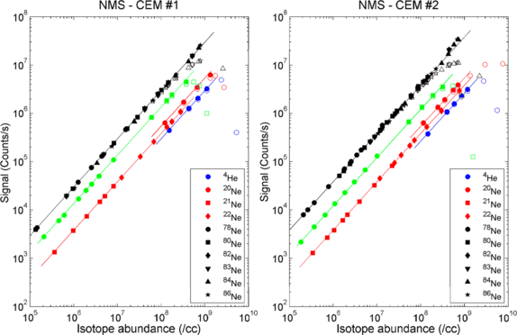

Linearity of the Channel Electron Multipliers (CEMs) for He, Ne, Ar, and Kr collected using the closed source with a filament emission of 200 μA. Clear symbols are the raw CEM values while colored symbols are the dead time corrected values (up to the CEM roll over point). The bias voltage of the CEMs used to acquire this data ranges from −2500 V to −2860 V. The intercept each linear fit (bias from x=y line in the log-log scale) translates the sensitivity in log scale of the instrument for that given isotope. Note that ²⁰Ne sensitivity is different from that of ²¹Ne and ²²Ne. This is due to the frequency change that occurs at 20.5 amu

Fig. 18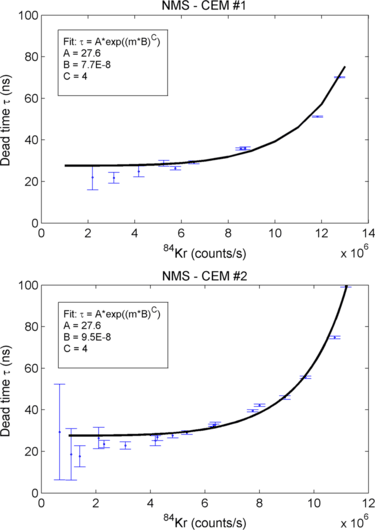

Variation of the dead time correction with count rate for the Channel Electron Multipliers (CEMs) derived using Kr measurements. The coefficient of the exponential fit are provided for each detector

Pulse Height Distribution: :

The NMS instrument pulse height discriminator is commanded by an 8 bits DAC and provides 255 level of discrimination. The CEM bias voltage was decreased progressively from −2400 V during instrument integration and was set to −2800 V during the first two months of the mission. Pulse height distributions were acquired regularly throughout the development and operation phases to verify the performance of the CEMs. Figure 19 presents comparisons between He pulse height distributions for CEM #1 and #2 for bias voltages ranging from −2800 V to −2400 V. This pulse height distributions were acquired during the checkout phase of the instrument (few days after launch) while it was still sealed. As expected the gain of each multiplier increases as the bias voltage decrease from −2400 V to −2800 V. Moreover these data shows that CEM #2 has a higher gain and a better performance than CEM #1 for the same bias voltage. During normal operations, the discriminators of both detector chains were set to 28 DAC units, low enough to allow the discriminator to capture the majority of the multiplier pulses, but high enough to reject any low level noise that may trigger false counts. The bias voltage for both multipliers was set to −2800 V.

Fig. 19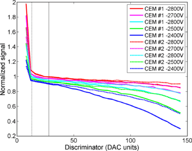

Pulse height distributions (PHDs) for CEM #1 and #2 using He. These PHDs were acquired at various bias voltages. The dotted line indicates the minimum discriminator setting that allows an effective noise rejection. The solid line indicated the discriminator setting used during nominal operations

Noise level in the detector chain: :

The instrument was designed to minimize the noise level in the detector chain. This goal was achieved by a careful isolation of the multipliers from any stray electrons that originate in the ionization sources. Moreover, the detector electronics were placed at a very short distance from the multipliers to minimize noise pickup. Noise levels in the active detection chain were assessed by turning on the closed source while configuring the switching lenses to select the open source. In that configuration all recorded counts can be assumed to be noise. During instrument checkout the noise level on both detection chains were found to be less than 8 counts/min.

Instrument Chemical Background

During integration the sensor underwent a multi-day high temperature bake out to insure the cleanliness of the internal surfaces and to minimize chemical background. Shortly after the ejection of the breakoff cap assembly, the instrument was assessed for the level of residual instrument background induced by internal surface outgassing, getter outgassing, filament outgassing, or spacecraft contamination. While this background tend to decay as the cumulative operational time of the instrument increases, the level and the nature of this background sets the detection limits of the instrument. Figure 20 shows the instrument background as it was measured in the first 3 months of the mission. This measurement is done by pointing the instrument boresight to the anti-ram direction. Filament outgassing is the source of most of the background in m/z 12–18, 28, and 44. Surface and getter outgassing are responsible for the residual water and for most of the hydrocarbon fragments seen in the spectra from both sources. As expected, the background in most mass channels decayed exponentially and was reduced by many several order of magnitudes after the first 3 months in space.

Fig. 20

Instrument background in the closed and open source modes collected at various days after the deployment of the breakoff assembly. Total time refers to the elapsed time since breakoff assembly while operation time refers to the cumulative time during which the filaments were on

One would notice the much lower background level in the open source compared to the closed source. This lower background is the result of the presence of a 1 V retarding potential grid that rejects most thermal ions (energy below 1 eV). This electrostatic background suppression increases the SNR of the open source for energetic exospheric neutrals that may be the result of surface sputtering processes.

Although its apertures had no direct geometric views of the spacecraft, it was still possible the instrument chemical background could be influenced by the self-scattered flux of various molecular species outgassed from the spacecraft. These species were dominated by water vapor, which in high vacuum readily effuses from non-metallic materials contained within various electronics units, multilayer insulation blankets, and even the spacecraft structure itself. Based on an analytical development by Robertson from the Bhatnagar-Gross-Krook approximation to the Boltzmann equation (Robertson 1976), a relationship was developed that linked this sensitive chemical background contribution to limits on spacecraft outgassing of water vapor. Even accounting for the exposure history of LADEE to the high vacuum of space prior to commencement of operations, predictions indicated this limit could only be met if all bus gaps were sealed and a dedicated vent was incorporated into the spacecraft design to allow water vapor from internally-carried sources to be directed radially away from the observatory on the side opposite NMS.

Instrument Sensitivity

The instrument sensitivity was initially measured in a static mode for He, Ne, Ar, Kr and Xe. In a static mode, the gas is leaked into the ionization source at a very low pressures and left to equilibrate before pressure readings are taken by an external stable ion gage while the corresponding instrument response is recorded. The measurements from the instrument are processed for dead time correction and background subtraction. After the sensor was pinched off sensitivities was continuously tracked using the noble gas mixture that was sealed in the instrument. The last direct sensitivities measurement for several multiplier voltage settings was conducted prior to the break-off cap ejection. This set of flight data was used to update the sensitivities that were established during ground calibration for the multiplier voltage and discriminator setting chosen for flight. The sensitivities in the closed source mode for the three key exospheric species (He, Ne and Ar) are provided in Table 3. Closed source normalized sensitivity S _n for another species s of mass m _s and electron ionization cross section (at 70 eV) σ _s can be derived through interpolation of the normalized sensitivities of Table 3 as a function of mass. To derive an absolute sensitivity S _a for the species, the normalized sensitivity S _n needs to be corrected for RF frequency and for ionization cross-section as:

$$S_{a} = S_{n} * C_{RF} ( m_{s} )* \sigma_{s} $$

where C _RF is a sensitivity correction factor:

$$C_{RF} = \left \{ \begin{array}{l@{\quad}l} 0.71& \mbox{if}\ m_{s} \leq20.5\\ 1.00& \mbox{if}\ m_{s} >20.5 \end{array} \right . $$

The sensitivity of the open source cannot be directly derived using the encapsulated calibration gas but will be determined in flight by comparing the count rates for exospheric He, Ne, and Ar that were collected alternately using the closed and the open source.

Table 3 NMS closed source sensitivities for He, Ne and Ar

Sensitivity Dependence with Temperature

The NMS sensitivities will drift from the values given in Table 3 as the instrument electrical and mechanical components warm up from dissipated electrical energy. This sensitivity variation is mainly due to two sources:

• 1. Shifting of the position of mass peaks due to RF thermal drift.

• 2. Thermomolecular pressure difference that forms between the hot closed source and the much cooler sensor.

RF thermal drift: :

Due to fringe field effects in the quadrupole rods, the transmission of the mass filter varies for small excursions from the center target mass. This creates small structures in any given mass peak. As the RF electronics warms-up the AC and DC analogue outputs drift slightly. These voltage drifts will slightly shift (up to 0.2 Da) the selected mass on the targeted peak and consequently the observed count level. If the density of the measured gas is constant, this drift will show as a sensitivity change for the measured species (Fig. 21).

Fig. 21

Example of sensitivity variation due to mass peak shape drifts

The amplitude of these sensitivity changes are temperature and mass dependent. Table 4 presents the maximum perceived sensitivity change as measured during the NMS thermal qualification tests. During those tests the instruments was operated at varying temperatures (from −30 ^∘C to +50 ^∘C). The sensitivity variations values provided in Table 4 should be taken into consideration when calculating the uncertainty of the NMS measurement.

Table 4 Maximum sensitivity variation observed during NMS thermal qualification (−30 ^∘C to +50 ^∘C)

Thermomolecular pressure difference: :

The instrumental effects on sensitivity discussed above relate to the efficiency of conversion of gas in the closed source to ions and thence to detector counts. In as much as NMS operation requires a hot filament, there is a wide range of temperatures within the instrument, which, in turn, results in a non-uniform distribution of gas density. The equivalent of hydrostatic equilibrium for a collisionless gas in a bounded system like the closed source and its appendages is nc=constant, where n is local gas density and $c= \sqrt{kT/2\pi m}$ is one-fourth the mean thermal speed of atoms of mass m. The effective gas temperature T is a local average of internal surface temperatures.

At the interface of the closed source entrance and the lunar exosphere the flux of atoms out of the instrument is $n_{CS} \sqrt{k T_{CS} /2\pi m}$ and the influx from the exospheric influx is

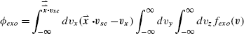
where the x-axis coincides with the axis of the field of view of the CS, is a unit vector in the +x direction, v _sc is the spacecraft velocity, and f _exo is the exospheric velocity distribution function. If f _exo is approximated as Maxwellian, the evaluation of the integrals is trivial, and the influx to the CS can be expressed as

$$\phi_{exo} = n_{exo} v_{eff} $$

where the effective velocity is

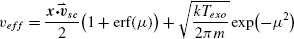
, n _exo is the exospheric concentration, and m is atomic mass.

In other words, the relationship of detector output, δ (counts per second), to the concentration of atoms in the exosphere is

$$n_{exo} = \frac{\delta}{S_{a} v_{eff}} \sqrt{\frac{k T_{CS}}{2\pi m}} $$

The time dependence of the temperature of the closed source, T _CS , as it is heated by the active filament has been determined from a dedicated sequence of repeated measurements of the ³⁶Ar peak, in flight but before the cap was ejected. Results of this experiment are shown as dots in Fig. 22. The data are interpreted as

$$n_{CS} = n_{0} \sqrt{{T_{CS}} / {T_{0}}} $$

and the subscript 0 identifies initial conditions. The underlying curve is

$$n_{0} \bigl[ 1+ \alpha \bigl( 1- e^{-t/\tau} \bigr) \bigr]^{-1/2} $$

where t is time from filament turn-on, α=0.6591, and τ=676.48 s. The fit is sufficiently strong to suggest that

$$\frac{T_{CS} (t)}{T_{0}} =1+ \alpha \bigl( 1- e^{-t/\tau} \bigr) $$

is a good approximation for modes of operation wherein only the CS is active, and the CS is active continuously.

Fig. 22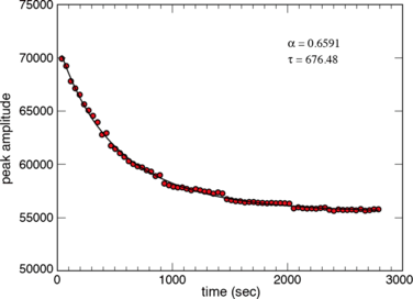

Sequential CS measurements of ³⁶Ar in detector counts per second prior to cap ejection. Time is measured from the application of power to the filament

4 Instrument Operations and Expected Results

4.1 Overview of NMS Measurement Modes

NMS measurement scenarios that impact the spacecraft attitude are RAM, TILT, WAKE, and ION campaigns. In the RAM mode the spacecraft points the NMS closed source inlet along the velocity vector and the spacecraft rotates at 1 revolution per orbit. This mode is the primary mode for measurement of He and Ar and other inert species and the wide field of view of the closed source allows a relaxed 2 degree pointing requirement. WAKE is designed to allow instrument background measurements to be made by pointing the NMS 180 degrees away from RAM. LExS models show that a negligible flux of gas enters the closed source in this configuration. TILT mode is intended to optimize open source measurements for sputtered species that would not be detected after a collision with a surface in the mass spectrometer. A typical tilt away from RAM pointing of the open source axis would be 30 degrees toward nadir although other tilt angles are possible to optimally match the sputtered velocity with the spacecraft orbital velocity of 1.6 km/sec. Particles with energies of greater than ∼25 eV will not be detected by the NMS in the open source mode at the nominal settings of the quadrupole deflector (Fig. 5). ION mode to reorients the axis of the spacecraft perpendicular to the orbital plane to search for ions in the NMS open source. Ions are only expected to be detected if the magnetic field happens to be in a direction that enables pick up ions to flow into the open source.

4.2 Commanding and Operations Overview

Operationally, since power sharing is required, the instrument is only powered for ∼48 minutes for observations. During this time the instrument is powered on, loaded, configured, and started for the science scenario, and then powered off again at the end of the window. All operations must be guided within this window. During the early checkout and commissioning phases, this restriction is not needed and functional testing is allowed longer durations; such as the CPT. The NMS operation is thought of in two separate disciplines: the commanding performed to the instrument and the data received from the instrument. Figure 23 shows the general overview of the end-to-end paths for each of these functions.

Fig. 23

The command and telemetry paths to the NMS from the Instrument Operations Center (IOC) shown in the bottom right, to the Science Operations Center (SOC), the Mission Operations Center (MOC), the uplink station, and the spacecraft command and data handling system (SC CDH) to the NMS. As illustrated, scripts can also be retrieved from the spacecraft memory and downloaded to the memory of the NMS

Commanding

The primary mode of commanding the instrument is through stored files of commands and code functions called scripts. There are two comprehensive scripts, one functional and one science, which define all operations desired for the instrument in a modular format. This allows loading smaller configuration scripts to define how the operations will be executed (i.e., which modules to execute). The functional script is stored in EEPROM and config files are loaded to define checkout activities, from as simple as an aliveness check to a comprehensive performance test. As would be expected, the science configurations orchestrate the collection scenarios throughout the lunar orbits, by interacting much more intensively with the hardware in setting the various DACs, etc. The script processor is and adaptation of that developed for SAM commanding and is a small, portable system that enables implementation of complex measurement sequences without the generation of new low level code. The scripting language provides access both to the NMS count data and to all housekeeping data. It is integrated with the alarm handler and incorporates a scriptable timer for periodic operations. A library is included for commonly used functions. The script processor enables rapid changes to flight sequences should this be desired.

Individual commands are also used for the instrument, to perform pre-defined functions, such as loading memory or controlling the execution of scripts. A more general RAW command is also used for invoking subfunctions that are not easily defined ahead of time. These database-defined commands use an upload execution code to define what priority the FSW needs to give to the execution (i.e., store for later or execute immediately).

Commanding is handled operationally in three ways, each allowing a slightly different functionality:

• 1. Individual commands either directly from the ground to the instrument, or from the CDH to the instrument on invocation of stored sequences of commands in spacecraft memory.

• 2. Script files that are loaded to the instrument and invoked, either directly from the ground or from the CDH on invocation of stored sequences of commands in spacecraft memory.

• 3. Script files previously loaded to the instrument invoked from the EEPROM.

Individual Commands

Transmission of individual commands (Sequence 1 in Fig. 23) allows more conservative stepping of procedures and insight to success and end-item verification. From the GSE, these commands are transmitted through use of ITOS, resident in the IOC via a VM connection (see GSE section). They are defined in the Project database and selected through a GUI interface. It is also possible that commands can be sent from sequences stored in spacecraft memory, called Relative Time Sequences (RTSs). These are generated using ITOS features and the database to compile the files and upload them to the Observatory for later use. This allows activities requiring sequences of commands to be performed more easily and with less reliance on solid communication with the MOC.

Scripts by ‘Load-and-Go’

The primary commanding of the instrument is via loading the desired script(s) to the instrument memory and commanding it to execute; coined ‘load-and-go’ execution (Sequence 2 in Fig. 23). This can be accomplished from the ground or from RTS. If commanded from the ground, the prime script is transmitted to instrument memory, followed by the configuration script, then the command to execute is sent. If performed via RTS, the scripts are loaded to the instrument-designated directory in spacecraft memory, the RTS(s) is loaded to the correct slot in spacecraft memory, and then the RTS is executed to load the scripts and execute the sequence.

Scripts from Memory

Scripts can also be stored in the instrument memory, then commanded to RAM and started (Sequence 3 in Fig. 23). This is the method used when executing functional tests. Functional tests are primarily used during the initial checkout activities after launch. This can be performed from the ground or via RTS. The primary script is loaded to RAM, the configuration script applied, and then the command is sent to begin the activity.

Planning Activities

In order to ease the complicated sequencing needed between subsystems and entities to perform a successful science collection scenario, the scenarios are defined through use of activities in the LASS planning tool. These activities dictate the RTS required, script files needed, pre and post sequences needed (such as power on/off), Observatory attitude required, data rates, etc. An activity is the comprehensive inclusion of all required resources for success. This is translated into the entire series of commands to orchestrate the end-to-end operation of that science scenario. For NMS, these scenarios are defined as the RAM, TILT, WAKE, and ION campaigns.

Product Configuration Management

As with all efforts, an important aspect is the control of that effort to ensure consistency and safety of the instrument. All scripts used for the FM are verified via the team CM process; requiring first review of the script. Following completion of that gate, it is initially placed in the SVN repository and execution on the breadboard is carried out. Once verified as safe from doing harm to the instrument, it is tested on the EM. After successful completion of this process, the script is finalized in the SVN system and marked ready for flight. The script is then transferred to the MOS SVN repository to await approval and implementation.

Telemetry

Telemetry is received by two different methods: real-time dataflow to the IOC and post-event file retrieval.

Only housekeeping telemetry is received during real-time contacts. This data is passed from the MOC, through the SOC, to the IOC in CCSDS frames (acronyms referenced in Table 5). At the IOC, the ITOS VM both unpacks the NMS Instrument Transfer Frames (ITF’s) and transfers to the LADEE GSE software for processing, and processes some of the data for display itself. This data is used for assessment of the health of the MEB and QMS. Both OTPS and LADEE GSE software packages allow limit checking and plotting besides the usual conversion displays.

Table 5 Acronyms

All NMS data, housekeeping and science, is downloaded from the Observatory and stored in separate files of CCSDS frames on the MOS file system for retrieval. These files are retrieved and processed into NMS ITF format for acceptance by the various analysis tools and databases.

‘GOLD’ Dataset

The retrieved science data dump files retrieved from the MOS file system are used to create the comprehensive dataset for the science collection, known as the ‘GOLD’ dataset. This is then submitted to the repository and fed to a database for use by the LADEE science team.

4.3 Data Archiving

The full set of NMS data will be archived in the atmospheres node of the Planetary Data System within 4 months of the end of the mission. The NMS archived data will include all detector count data for each m/z value sampled and will include the full set of NMS housekeeping data that enables the commanding of the instrument to be understood. Data generated by the NMS instrument will be organized in products according to their processing state and will adhere to the nomenclature of product definition set by the LADEE project. The NMS pipeline processes the Packet Data (binary files as generated by the instrument) to generate the Raw, and Calibrated products that will be archived at the PDS (Table 6).

Table 6 Data definitions for NMS

The Packet Data will be separated by telemetry channel (Housekeeping, Science and Instrument Log) and converted to ASCII to generate the Raw Housekeeping, the Raw Science and the Message Log. These data will be checked for anomalies and will be time-stamped. The Housekeeping units will be expressed in engineering units (Volts and Digital Numbers) when applicable.

Then, the Raw Science will be corrected for detector response (dead time correction) and the Raw Housekeeping will be converted to scientific units (physical unit corresponding to the measurement being made: for example deg C for Temp, A for current or emission, and V for voltage monitor circuits) when applicable. These data will be checked for anomalies and the time-stamp will be corrected for any offset between the instrument and spacecraft clocks. This process will yield Calibrated Housekeeping and Calibrated Science ASCII files.

4.4 Summary

The extended LADEE mission duration that extends coverage for the LDEX, UVS, and NMS instruments through multiple lunations together with regular measurements at tens of kilometers above the surface is intended to enable the variability of both gas and dust in the lunar exosphere to be explored. The observations of emissions many kilometers above the surface by the Apollo astronauts may be better understood after this mission and the lunar environment better characterized before humans again return to the moon and further perturb this tenuous atmosphere. The NMS and UVS will provide complementary measurements for variations in the known gases (He, Ar, Na, K) the search for new species with NMS targets including He and Ar and UVS targets Na and K and both instruments searching for yet to be measured gases such as CH₄, CO, CO₂, H, H₂O, N, C, S, Si, Al, Ca, Fe, Ti, Al Mg, OH or reductions in their upper limits. The detailed characterization of a surface boundary exosphere should enable better predictions of the space environment around the many similar objects in our solar system.

References

A. Fahey, Measurements of dead time and characterization of ion counting systems for mass spectrometry. Rev. Sci. Instrum. 69, 1282 (1998)
R.R. Hodges Jr., Applicability of a diffusion model to lateral transport in the terrestrial and lunar exospheres. Planet. Space Sci. 20, 103 (1972)
R.R. Hodges Jr., Paper presented at the Lunar and Planetary Science Conference Proceedings, n/a 1, 1980
R.R. Hodges Jr., J.H. Hoffman, Measurements of solar wind helium in the lunar atmosphere. Geophys. Res. Lett. 1, 69 (1974)
R.R. Hodges Jr., J.H. Hoffman, Paper presented at the Lunar and Planetary Science Conference Proceedings, n/a 1, 1974
R.R. Hodges Jr., F.S. Johnson, Lateral transport in planetary exospheres. J. Geophys. Res. 73, 7307 (1968)
R.R. Hodges, Ice in the lunar polar regions revisited. J. Geophys. Res., Planets 107, 6-1 (2001)
R.R. Hodges, Resolution of the lunar hydrogen enigma. Geophys. Res. Lett. 38, 6201 (2011)
R.R. Hodges, J.H. Hoffman, F.S. Johnson, The lunar atmosphere. Icarus 21, 415 (1974)
W. Kasprzak et al., Paper presented at the Society of Photo-Optical Instrumentation Engineers (SPIE) Conference Series, October 1, 1996
P.R. Mahaffy, Characteristics of an electrostatic quadrupole deflector. J. Vac. Sci. Technol. 8, 3244 (1990)
P.R. Mahaffy et al., The sample analysis at Mars investigation and instrument suite. Space Sci. Rev. 170, 401 (2012)
H.B. Niemann et al., Pioneer Venus Orbiter neutral gas mass spectrometer experiment. IEEE Trans. Geosci. Remote 18, 60 (1980)
H.B. Niemann et al., Galileo Probe Mass Spectrometer experiment. Space Sci. Rev. 60, 111 (1992)
H.B. Niemann et al., The Planet-B neutral gas mass spectrometer. Earth Planets Space 50, 785 (1998)
H. Niemann et al., Paper presented at the Huygens: Science, Payload and Mission, n/a 1, 1997
R. Rejoub, B.G. Lindsay, R.F. Stebbings, Determination of the absolute partial; and total cross sections for electron-impact ionization of the rare gases. Phys. Rev. A 65, 042713 (2002)
S.J. Robertson, BGK model solution of back scattering of outgas flow from spherical spacecraft. Prog. Aeronaut. Astronaut. 51, 1 (1976)
N.W. Spencer, G.R. Carignan, In situ measurements of thermospheric composition, temperature, and winds by mass spectrometry. Adv. Space Res. 8, 107 (1988)
S.A. Stern, The lunar atmosphere: history, status, current problems, and context. Rev. Geophys. 37, 453 (1999)
J. Veverka et al., Comet nucleus tour. Acta Astronaut. 35, 181 (1995)
J.H. Waite et al., The Cassini Ion and Neutral Mass Spectrometer (INMS) Investigation. Space Sci. Rev. 114, 113 (2004)
P.B.A. Wurz, V. Coffey, B.K. Dichter, W.T. Kasprzak, A.J. Lazarus, W. Lennartsson, J.P. McFadden, in ISSI Scientific Report, ed. by M.E.S. Wuest, R. von Steiger. International Space Science Institute (2007)
A. Yaniv et al., Paper presented at the Lunar and Planetary Science Conference Proceedings, n/a 1, 1972
Acknowledgements
The NMS development was funded by the Science Mission Directorate of the National Aeronautics and Space Administration.
Author information
Authors and Affiliations
Corresponding author
Rights and permissions
Open Access This article is distributed under the terms of the Creative Commons Attribution License which permits any use, distribution, and reproduction in any medium, provided the original author(s) and the source are credited.
About this article
Cite this article
Mahaffy, P.R., Richard Hodges, R., Benna, M. et al. The Neutral Mass Spectrometer on the Lunar Atmosphere and Dust Environment Explorer Mission. Space Sci Rev 185, 27–61 (2014). https://doi.org/10.1007/s11214-014-0043-9
Received:
Accepted:
Published:
Issue Date:
DOI: https://doi.org/10.1007/s11214-014-0043-9