The Search-Coil Magnetometer for MMS

Abstract

The tri-axial search-coil magnetometer (SCM) belongs to the FIELDS instrumentation suite on the Magnetospheric Multiscale (MMS) mission (Torbert et al. in Space Sci. Rev. (2014), this issue). It provides the three magnetic components of the waves from 1 Hz to 6 kHz in particular in the key regions of the Earth’s magnetosphere namely the subsolar region and the magnetotail. Magnetospheric plasmas being collisionless, such a measurement is crucial as the electromagnetic waves are thought to provide a way to ensure the conversion from magnetic to thermal and kinetic energies allowing local or global reconfigurations of the Earth’s magnetic field. The analog waveforms provided by the SCM are digitized and processed inside the digital signal processor (DSP), within the Central Electronics Box (CEB), together with the electric field data provided by the spin-plane double probe (SDP) and the axial double probe (ADP). On-board calibration signal provided by DSP allows the verification of the SCM transfer function once per orbit. Magnetic waveforms and on-board spectra computed by DSP are available at different time resolution depending on the selected mode. The SCM design is described in details as well as the different steps of the ground and in-flight calibrations.

1 Introduction

The Magnetospheric Multiscale mission aims at increasing our understanding of major fundamental plasma physics processes such as magnetic reconnection, particle acceleration and turbulence (Burch 2014). In a collisional plasma, binary collisions between particles ensure that plasma dynamics is adequately described by a fluid-like theory such as the magnetohydrodynamics (MHD). Then binary collisions can generate a diffusion across the magnetic field leading to a net plasma transport or a dissipation allowing magnetic reconnection to occur. However, in the Earth’s magnetosphere the mean free path for binary collisions between particles is larger than the size of magnetosphere and the plasma can be considered as collisionless. In absence of collisions, particles can still interact with fluctuating electromagnetic fields giving rise to anomalous resistivity and anomalous transport. These electromagnetic fields can be related to waves, microinstabilities or turbulence. Thus accurate measurements of electromagnetic fluctuations are crucial to investigate the dynamics of basic processes in collisionless plasmas (Torbert et al. 2014). The tri-axial search-coil magnetometer (SCM) together with the spin-plane double probe (SDP, Lindquist et al. 2014) and the axial double probe (ADP, Ergun et al. 2014) provide the three-dimensional electromagnetic fields up to 6 kHz. All these analog waveforms are digitized by the digital signal processor (DSP) then transmitted to the central data processing unit (CDPU) within the Fields central electronics box (CEB), together with the two waveforms provided by the analog fluxgate (AFG) and digital fluxgate (DFG) magnetometers (Russell et al. 2014) and data from the electron drift instrument (EDI, Vaith et al. 2014). The time synchronization of all Fields components has been carefully investigated and is described in a companion paper (Torbert et al. 2014). Finally, all fields as well as particle measurements are collected and stored by the central instrument data processor (CIDP) which also provides power, time synchronization signals and commands. The MMS SCM has been designed and built by the Laboratoire de Physique des Plasmas (LPP). It has a long heritage and its relatives are still working nominally in the solar system onboard the Cassini (Gurnett et al. 2004), Cluster (Cornilleau-Wehrlin et al. 1997, 2003) and THEMIS (Roux et al. 2009; Le Contel et al. 2008) missions.

As was done for the Cluster mission, the four MMS satellites will evolve in a tetrahedral configuration in order to estimate electric current densities as well as other gradients of the medium (density, temperature, pressure) but will cover smaller intersatellite distances from 10 to 100 km. While Cluster satellites follow a polar orbit, MMS spacecraft (s/c hereafter) will have an equatorial orbit in order to optimize the crossing of the key regions such as the equatorial subsolar region and the central region of the magnetotail. From the point of view of the wave measurements, it will allow a characterization of electromagnetic waves with smaller wavelengths compared to those investigated by the Cluster mission which scanned larger intersatellite distances. As waves with short wave lengths can be more sensitive to Doppler shift effect related to fast flowing plasma, their analysis will benefit from the high-time resolution of the particle measurement (150 ms for the ion moments).

In the next section, the main science objectives, as well as the SCM requirements, are presented. In Sect. 3, the principle of the instrument is explained and MMS SCM design (sensor and preamplifier) is described in details in Sect. 4. Calibration and testing are presented in Sect. 5. Finally, Sect. 6 summarizes the different SCM operational modes, data products and on-board calibration sequence.

2 Science Objectives and Requirements

One of the main science objectives of the MMS mission is to provide a thorough description of the physical mechanisms which can lead to the reconnection of magnetic field lines within and around the Earth’s magnetosphere. Indeed, the magnetic energy can be transferred to the plasma via the magnetic reconnection, thereby leading to particles acceleration and heating. Furthermore, on the dayside, magnetic reconnection can allow the solar wind plasma to penetrate into the magnetosphere, crossing the otherwise closed magnetopause boundary. In the night side, it can allow the fast transport of the plasma from the mid-magnetotail, the assumed location of the reconnection region, toward the quasi-dipolar near-Earth tail and contribute to the ejection of plasmoid/flux rope in the far tail. In the framework of the Hall magnetic reconnection model, the decoupling between the magnetic field lines and the particles happens at different scales for ions and electrons (Birn et al. 2001, and references therein). In the absence of a finite guide field, the sizes of the different regions correspond to the inertial lengths of ions and electrons while with a finite guide field, ions are demagnetized at the effective gyration (Larmor) radius scale (Hesse et al. 1999; Pritchett and Coroniti 2004, and references therein). Inertial effects are therefore considered as the dominant effect allowing the reconnection to occur. Yet, in the smallest (electron) diffusion region, the dynamics is thought to be controlled by whistler or kinetic Alfvén waves (KAW) depending on the presence of a finite guide field (Mandt et al. 1994; Rogers et al. 2001; Drake et al. 2008). These waves could accelerate the electrons outside the electron diffusion region and enable fast magnetic reconnection.

Another way to get the decoupling between the magnetic field and the particles in a collisionless plasma, is to consider the interaction of the particles with the electrostatic/electromagnetic fluctuations. Such field fluctuations can rise from waves, local micro-instabilities and/or turbulence. This interaction with electrostatic (Tsurutani and Thorne 1982) or electromagnetic fluctuations (e.g., Perraut et al. 1979; Gendrin 1983; Chaston et al. 2008) can allow the plasma to diffuse through the magnetic field lines leading to the so-called anomalous diffusion. Anomalous diffusion may, or may not, evolve toward a stationary regime of the system. These wave/particle interactions can also produce an anomalous plasma resistivity and then make collisionless magnetic reconnection possible (Huba et al. 1977). Micro-instabilities such as current-driven instabilities with large growth rates can also directly trigger larger scale modification of the magnetic field configuration and generate strong electromagnetic fluctuations in a broad frequency range (e.g., Lui et al. 1996; Daughton 1999). Finally, these interactions can also lead to the formation of non-linear coherent structures which can modify the plasma equilibrium and the transport of mass, momentum and energy (e.g., Cattell et al. 2005; Parks et al. 2007; Andersson et al. 2009).

One specific aspect of natural collisionless plasmas confined by an external magnetic field—produced by the internal motion of the core materials of the planet or the star—is their dynamics which are based on periodic motions. Indeed, in addition to the classical gyromotion of the charged particles around the magnetic field lines, particles are bouncing back and forth along the magnetic field line between their mirror points and then drift around the central object (Northrop and Teller 1960; Roederer 1967). Each of these three periodic motions can lead to resonant interactions between particles and electromagnetic waves with frequencies matching these periodic oscillations (Tur et al. 2010; Fruit et al. 2013, and references therein). Furthermore, the fast bouncing motion of electrons (due to their small mass) along the magnetic field is able to neutralize any charge separation due to differential perpendicular motion between ions and electrons. As a consequence, a quasi-static electric field can easily be shielded by electrons and the plasma transport can be inhibited (Pellat et al. 1994; Le Contel et al. 2000, 2001). The low frequency eigenmodes of these periodic systems are quite difficult to identify (e.g., Chen and Hasegawa 1991; Hurricane et al. 1995). Such effects do not occur when the frequency of the perturbations is larger than the particle bounce frequency; then a fluid approach can safely be used to describe plasma dynamics (Weiland 2000). They can be also ignored if electrons are prevented from bouncing, for instance due to interaction with some electromagnetic waves (Le Contel et al. 2001). The Earth’s magnetotail is a classical example of collisionless and magnetically confined plasma. In the dayside, the situation is even more complex as it corresponds to the interaction between a cold, dense and large scale plasma (the solar wind/magnetosheath plasma) and a hot, dilute plasma confined at smaller scale by the Earth’s magnetic field: a very asymmetric system. Therefore, in the night side as well as in the dayside, plasma acceleration, transport or turbulence are physical processes which are far from being fully understood.

Whatever the physical process and the chosen model, it is therefore crucial to ensure comprehensive measurements of the 3D electromagnetic fields in an extended frequency range from the quasi-MHD domain (∼ mHz) to high frequency waves (∼ kHz). Thanks to polarization analyses based on magnetic field measurement (e.g., Means 1972; Samson and Olson 1980) and to estimates of the wave phase velocity from the ratio between the amplitudes of electric and magnetic components, these different mode waves can be identified. Well synchronized measurements of the magnetic and electric fluctuations also allow calculation of the Poynting vector and determination of the source and the direction of propagation of waves.

There is also a strict alignment requirement that arises out of the need to resolve temporal and spatial structures as measured by the four MMS spacecraft. The Cluster mission has shown that for waves with large wave vectors, the wave frequency in the s/c frame can be strongly Doppler-shifted. This was demonstrated using the k-filtering technique that determines the wave vector as function of frequency. This technique needs to assume the time stationarity and the spatial homogeneity of the time series at least at the scale of the analyzed period (Pinçon and Lefeuvre 1991; Sahraoui et al. 2003). Thus, at the dayside with the shocked solar wind plasma of the magnetosheath as well as in the nightside during fast plasma transport periods, the analysis of the small wave length fluctuations requires a high time resolution measurement of the ion velocity in order to move the data from the s/c frame to the plasma frame. Finally, such an analysis also requires that any phase shift introduced either by the misalignment between the magnetometers axis and the s/c axis or by a time inaccuracy δt between s/c measurements are no larger than few degrees (Pinçon and Lefeuvre 1992; Sahraoui et al. 2003).

Since the wave power is known to be quite large during sudden magnetospheric reconfiguration events in the nightside as well as in the dayside, there was no need to have a SCM sensitivity better than those of Cluster and THEMIS search-coils. On the other hand, the SCM allocated mass was very stringent. Thus the MMS SCM is designed to reduce the mass, as compared to THEMIS for instance, without reducing too much the sensitivity. Therefore the SCM requirements are a tradeoff between mass and sensitivity.

2.1 Dayside Region

The understanding of the mechanisms by which the solar wind plasma can penetrate into the magnetosphere through the magnetopause dayside or/and flanks is still a matter of debate. Magnetic reconnection, diffusive (Tsurutani and Thorne 1982; Gendrin 1983; Chaston et al. 2008) and impulsive penetration (Lemaire 1977; Sibeck 1990), Kelvin–Helmholtz instability (Sckopke et al. 1981; Hasegawa et al. 2004; Smets et al. 2007) are physical mechanisms which are still extensively studied (see Phan et al. 2005 for a detailed review). Again, whatever the mechanism the electromagnetic fluctuations are thought to play an important role (anomalous resistivity, anomalous transport across the magnetic field, acceleration and heating).

The level of magnetic fluctuations at the magnetopause is known to be higher than in the magnetosheath. For instance in the ultralow-frequency range (ULF: 0–10 Hz) it can reach an integrated power about 100 nT² whereas from 5 Hz to 1 kHz almost in the extremely-low frequency (ELF: 10 Hz–3 kHz) range, it was measured about 1 nT² (Gurnett et al. 1979; Perraut et al. 1979). Magnetic spectral densities were measured up to $300~\mbox{pT/}\sqrt{\mbox{(Hz)}}$ by GEOS-2 s/c in the 0–10 Hz frequency range (Rezeau et al. 1986, 1989). More recently, a statistical study from Cluster data suggests that the ULF wave integrated power at the magnetopause depends upon the ULF integrated power of the magnetosheath waves and varies from 0.1 to 100 nT² (Attié et al. 2008). In the ULF/ELF range, lower-hydrid waves (mainly electrostatic), KAW and whistler mode waves have been identified as the main contributors of wave activity. While lower-hydrid waves were found in some cases to be intense enough to ensure significant resistivity (Cattell et al. 1995), the opposite was also concluded (Bale et al. 2002) except across thin current sheets (Vaivads et al. 2004). On the other hand, Doppler-shifted KAW amplitudes were shown (Chaston et al. 2008) to be also sufficiently large to provide cross-field diffusion at an equivalent collisional rate (Bohm rate). In these latter studies, magnetic spectral densities were measured about $10\mbox{--}100~\mbox{pT/}\sqrt{(\mbox{Hz})}$. Furthermore, KAW are invoked as a possible candidate to heat magnetosheath electrons along the ambient magnetic field in the magnetopause current layer (Roux et al. 2011). At higher frequency, large amplitude whistler mode waves were detected in association with thin current sheets (Stenberg et al. 2005) or magnetic field minima (Vaivads et al. 2004) and proposed as a tracer of the first opened magnetic lines during the dayside reconnection process; the corresponding magnetic spectral densities were about $30~\mbox{pT/}\sqrt{\mbox{(Hz)}}$.

2.2 Nightside Region

In the magnetotail, lower hydrid waves have been also invoked to provide anomalous resistivity needed in resistive magnetic reconnection models. As in the dayside observations, these waves were found not to be intense enough in some studies (Shinohara et al. 1998) while in others they reached a sufficient intensity to provide the necessary resistivity (Cattell and Mozer 1987). Shinohara et al. (1998) reported magnetic spectral densities larger than $30~\mbox{pT/}\sqrt{\mbox{(Hz)}}$ around 10 Hz. In the same ULF/ELF range but below the lower hybrid frequency, fast plasma flows detected in the magnetotail were shown to be associated with strong emissions of KAW which could be responsible for a significant energy loss from the flows (Chaston et al. 2012). At higher frequency, whistler mode wave emissions were often reported through the magnetotail in association with flux rope signatures or electron beams (Gurnett et al. 1976; Kennel et al. 1986; Zhang et al. 1999). More recently, these waves were detected during local near-Earth dipolarisation (Le Contel et al. 2009), dipolarisation front crossing (Khotyaintsev et al. 2011), mid-tail substorm activity (Wei et al. 2007) and trapped within non linear ion scale magnetic structures (Tenerani et al. 2012, 2013). All these measurements correspond to magnetic spectral densities about $10\mbox{--}100~\mbox{pT/}\sqrt{\mbox{(Hz)}}$ between 10 to 100 Hz and $0.1\mbox{--}0.03~\mbox{pT/}\sqrt{\mbox{(Hz)}}$ between 100 Hz to ∼1 kHz (about the local electron gyrofrequency). Finally, electron scale solitary waves (electrostatic as well as electromagnetic) have been identified in the magnetotail during substorm events thanks to waveform captures at very high sampling rates onboard Cluster (e.g., Cattell et al. 2005) or THEMIS satellites (Ergun et al. 2009; Andersson et al. 2009; Tao et al. 2011). These studies show that the magnetic component amplitudes associated with these non-linear structure can reach ∼50 pT–200 pT around 400–800 Hz.

2.3 Requirements

Thus, both dayside and nightside low-frequency wave emissions are expected to generate magnetic spectral densities larger than $2~\mbox{pT/}\sqrt{\mbox{(Hz)}}$ near the upper limit of the ULF range. Whistler mode waves which could play a crucial role during the reconnection process are expected to be emitted at higher frequency (f>20 Hz) in the ELF range and with spectral densities about $10\mbox{--}100~\mbox{pT/}\sqrt{\mbox{(Hz)}}$. At higher frequencies (∼800 Hz corresponding to 1.2 ms time scale), solitary waves which are detected during fast variations of the magnetic field configuration have magnetic amplitudes about 50 pT–200 pT. The SCM provides the three components of the magnetic fluctuations in the 1 Hz–6 kHz nominal frequency range which includes the lower hybrid wave and KAW frequency range as well as whistler mode waves (up to their cut off frequency equal to the electron gyrofrequency) and solitary waves. The noise equivalent magnetic induction (NEMI or sensitivity) of the search-coil antenna needs to be less than or equal to: $2~\mbox{pT/}\sqrt{\mbox{(Hz)}}$ at 10 Hz, $0.3~\mbox{pT/}\sqrt{\mbox{(Hz)}}$ at 100 Hz and $0.05~\mbox{pT/}\sqrt{\mbox{(Hz)}}$ at 1 kHz. The SCM resolution at 1 kHz has been fixed to 0.15 pT.

The mass allocated to the SCM sensor (including mounting structure and connector but without harness) and the preamplifier are 239 g and 222 g respectively. The SCM power allocation is 166 mW whatever the selected mode. Finally, The SCM shall meet performance requirements during science operations with a+z axis to spin axis misalignment of less than 1.0 deg. Also, the SCM sensor tube orientation with respect to the local SCM instrument coordinate system X-axis vector (directed along the magnetic boom) and Y-axis vector (aligned with the Z s/c axis), individually shall be less than ±0.2 deg to each vector, with an associated knowledge of ±0.2 deg. Note that the total timing uncertainty of the science measurements with respect to international atomic time (TAI) is required to be less than 500 microseconds.

In the next section, the SCM instrument is described in details and the SCM compliance with all these requirements is discussed.

3 Description of the Instrument

3.1 Magnetic Amplification

When a magnetic field H is applied on a ferromagnetic material, the latter becomes magnetized. In a linear, homogeneous and isotropic material, this magnetization M is linked to the magnetic field by M=χ H. It implies an increase in flux density B:

$$ \mathbf{B} = \mu_0 ( \mathbf{H} + \mathbf{M} ) = \mu_0 (1 + \chi ) \mathbf{H} = \mu\mathbf{H} $$

(1)

with μ ₀ (resp. μ) being the magnetic permeability of vacuum (resp. of the material), and χ the magnetic susceptibility. When magnetic field lines exit from the ferromagnetic core, a magnetic interaction appears which is opposite to the magnetic field. This interaction, named demagnetizing field $\mathbf {H_{d}}$, is related to the shape of the core through the demagnetizing coefficient tensor N _d and magnetization by

$$ \mathbf{H}_d = - \mathsf{N}_{d}\mathbf{M} $$

(2)

By combining (1) and (2), we can express the ratio between the flux density inside of the ferromagnetic body B _i and outside B _ext . This ratio μ _app , called apparent permeability, depends on the relative initial permeability of the ferromagnetic core μ _r =μ/μ ₀ and the demagnetizing field factor N _d,j in a given direction (j=x,y,z).

$$ \mu_{app,j} =\frac{B_i}{B_{ext}} = \frac{\mu_r }{1 + N_{d,j} (\mu_r -1)} $$

(3)

In the case of rods or cylinders with high aspect ratio m (i.e. m=length/diameter=L/d≫1), the formulas for ellipsoid given in Osborn (1945) allow to a good estimate of demagnetizing factor in the longitudinal direction (z) as N _d,z =(L(2m)−1)∖m ².

A way to increase magnetic amplification consists in the implementation of magnetic concentrators (Coillot et al. 2007) at the ends of the ferromagnetic core. Let us consider a ferromagnetic core of length L, with a diameter d in the central region and a diameter D at the two extremities (Fig. 1). The formula for apparent permeability becomes:

$$ \mu_{app,j} = \frac{\mu_r }{ 1 + N_{d,j}(L/D)\frac{d^2}{D^2} (\mu_r -1)} $$

(4)

For a given set of length, diameter and magnetic material, an increase in diameter of the magnetic concentrators will lead to a significant increase in apparent permeability. Coillot et al. (2007) report an increase in apparent permeability larger than 50 %. This increase allows a reduction of the number of turns of the winding, all things being equal. Thus the mass of the winding and the thermal noise due to the resistance of the winding will be reduced. To take advantage of this improvement, design of the sensor by means of mathematical optimization was implemented.

Fig. 1

Ferrite core and winding

3.2 Electrical Modeling of the Induction Sensor

The principle of the induction sensor derives from Faraday’s law. For N coils of section S, the voltage e is given by e=−Ndϕ∖dt, where ϕ is the magnetic flux through one coil. The voltage is proportional to the time derivative of the flux, thus the higher the frequency, the higher the output voltage will be (up to the limit of the resonance frequency of the coil). The use of a ferromagnetic core to increase the sensitivity leads to the following formula:

$$ e = - N \mu_{app} S \frac{d B }{dt} $$

(5)

where μ _app is given by (4) in the case of a magnetic concentrator and B is the magnetic flux density. The RLC elements of the equivalent circuit which has the same frequency behavior as the search coil antenna are sketched in Fig. 2. Explicit values of the resistance, the inductance and the capacitance can be found in Coillot and Leroy (2012). Note that in case of a multi layer winding the capacitance between layers will be preponderant compared with the capacitance between each coil. Then, assuming the temporal variations as ∝exp(jωt) the transfer function between the output of the measurable voltage and the flux density can be expressed as

$$ \frac{V_{out}}{B} = \frac{-j \omega N \mu_{app} S}{(1-\mathit{LC}\omega ^2)+jRC\omega} $$

(6)

It shows that the induced voltage will increase with the frequency up to the resonance of the induction sensor ($1/ \sqrt{\mathit{LC}}$). In order to measure natural plasma waves in a wide frequency range, this resonance has to be removed. This is why a flux feedback is implemented in the conditioning electronics, which allows a wide band coverage.

Fig. 2

Induction sensor equivalent electrical circuit

3.3 Electronic Conditioning of Induction Sensors by Means of Flux Feedback

A flux feedback low noise amplifier is used for MMS induction magnetometer. The flux feedback (Fig. 3) generates a flux opposite to the flux to be measured. It allows a removal of the main resonance. Alternative solutions using current amplifier are reported by many authors (e.g., Tumanski 2007). Both flux feedback and current amplifier provide an efficient removal of the first resonance and a flattening of the transfer function of induction sensors. In the case of the flux feedback amplifier, the output transmittance is

$$ T(j\omega)=\frac{V_{out}}{B} = \frac{-j \omega N \mu_{app} S G}{(1-\mathit{LC}\omega^2)+j(RC\omega+ M/R_{fb})} $$

(7)

where M is the mutual inductance between the measurement winding and the feedback winding, R _fb is the feedback resistance and G=(1+R2/R1) is the gain of the amplifier.

Fig. 3

Principle of search-coil with feedback loop

4 SCM Design

The SCM consists in a tri-axial set of magnetic sensors with its associated preamplifier box. The SCM sensor is mounted on the same five meter boom as the analog flux-gate magnetometer (AFG), 4 meters from the s/c. The SCM preamplifier box is mounted on the s/c deck (outside of the central electronics box) near the base of the AFG/SCM magnetometer boom. The SCM block diagram is shown in Fig. 4. The power (±8 V) is provided by the low voltage power supply (LVPS) within the CEB. The SCM preamplifier is connected to the digital signal processor (DSP) which digitizes and processes the three analog waveforms delivered by SCM as well as those delivered by SDP and ADP electric field antennas. Furthermore, all electromagnetic wave forms (SCM, ADP and SDP) corresponding to the low frequency part of the frequency range (f<6.5 kHz) are low pass filtered by analog filters (a 5 poles Bessel) implemented in the DSP. The filters have a cutoff frequency of 6.5 kHz at an amplitude −3 dB (±1 dB max) from the maximum pass band amplitude. Once per orbit, the DSP injects a calibration signal into the SCM. A thermistor mounted on the SCM structure provides the temperature measurement at the level of the SCM sensor (housekeeping).

Fig. 4

SCM block diagram

4.1 Sensor

The SCM sensor consists of three magnetic sensors mounted on a tri-axial structure (Fig. 5). This structure was designed to ensure a precise alignment of the sensors with respect to the satellite axis. The orthogonality of the three mechanical axis of this structure is better or equal to 0.05 deg in order to satisfy the final ±1 deg required between SCM and s/c axis. Yet, it has been found on FM2 unit that the torque applied on the screws fixing each sensor on the SCM structure leads to a small rotation of the structure and as a consequence of the Y and Z sensors around the X-axis. Thus the error of alignment between the SCM Y tube with respect to the Y-axis vector of the SCM coordinate system (corresponding to the Z spacecraft axis) has been measured larger than the required ±0.2 deg. This error has been precisely measured using 3D metrology for all FM except FM1 (already delivered). These alignment measurements will be used to build a correction matrix for post processing corrections. With regard to the FM1, in-flight intercalibrations between AFG/DFG and SCM (using spin modulation) on FM2, FM3 and FM4 will allow us to determine the FM1 correction matrix. These matrices will be included in the SCM calibration program. As explained in Sect. 3.1, the core of magnetic sensor is made of ferromagnetic material. Its characteristics (composition and shape) are optimized to obtain a high magnetic amplification with a low mass. The core length is 10 cm and the diameter 4 mm. Then a primary winding with a large number of turns (more than ten thousands) is implemented to collect the voltage induced by the time variation of the magnetic flux. Finally a secondary winding with a smaller number of turns provides a flux feedback. As discussed in Sect. 3.3, this feedback circuit allows a removal of the resonance and flattens the frequency response of the antenna. Furthermore flux feedback removes the phase variations associated with temperature variations.

Fig. 5

SCM FM1 tri-axial sensor with its pigtail connector

Internal electrostatic shielding is implemented around each antenna to minimize their sensitivity to electric fields. This electrostatic shielding is also reinforced by the multi-layer insulation or thermal blanket added to ensure the thermal isolation of the sensors. The mass of the SCM sensor including the tri-axis structure is 214 g.

4.2 Preamplifier

The three analog signals are routed to the SCM preamplifier via the SCM harness equipped with a silver-plated copper conductive shield braid. The SCM preamplifier, designed at LPP, has been realized in multi-chip vertical technology (hybrid) by the French 3D PLUS company (Fig. 6). Each channel has two stages of amplification. The first stage has a low-noise input and a gain of 46 dB. The second stage has a gain of 31.5 dB and ensures low and high-pass filtering. A power supply regulation is also implemented as well as a calibration buffer in order to receive the onboard calibration signal sent by DSP. The mass and the power consumption of the SCM preamplifier are 206 g (including the housing, mass of the 3D PLUS module being 37 g) and 130 mW respectively. SCM characteristics are summarized in Table 1.

Fig. 6

SCM FM1 preamplifier in its housing. The central golden square is the 3D PLUS cube that includes the three channels’ amplifiers and a power supply regulator

Table 1 Summary of SCM mechanical, mass and power characteristics

5 Calibration and Testing

5.1 Calibration and Testing Plan

The SCM sensor, pre-amplifier and harness have been calibrated for gain and phase at the national magnetic observatory of Chambon-la-Forêt. The facility already used for the search-coil calibration of the previous missions (Cassini, Cluster, THEMIS, hereafter called original facility) was no longer fully operational (2 axes were damaged) and moreover the gain measurement with the last single available axis was found to be biased up to almost ten percents (∼1 dBV/nT) above 1 kHz. A new three-axis system has been built by LPP simultaneously with the development and manufacturing of the SCM units. It consists of three large diameter Helmholtz coils (2 m) mounted on a polycarbonate structure to ensure a homogeneous magnetic field at the scale of the sensor and in the MMS SCM nominal frequency range 1 Hz–6 kHz (Fig. 7). The accuracy of the facility was verified using a sensor reference for which the theoretical transfer function is fully known. Yet, the new facility has been only ready for the calibration of SCM FM2 and following models. Thus SCM FM1 has been calibrated with the original facility. In order to check for the homogeneity of the SCM calibration and get rid of possible uncertainties, SCM FM2 has been calibrated using both test facilities.

Fig. 7

New system of three-axis Helmholtz coils at Chambon-la-Forêt

Furthermore, the in-flight intercalibration between AFG/DFG and SCM based on the use of the spin modulation (T _spin =20 sec) requires the measurement of the SCM transfer function at very low frequency; in the range of the spin frequency. SCM gain being very small at such low frequencies and the spectrum analyzer used to measure the transfer function being also less sensitive, a different calibration setup has been preferred for the lowest frequency range. It consists in using a single Helmholtz coil with a smaller diameter of 1 m but a larger number of windings. This latter equipment produces the larger magnetic field required to compensate for the small SCM gain at very low-frequencies. Gains and phases measured with these two different setups match within 0.1 dBV/nT (∼1 %).

5.2 Transfer Function of the On-Board Calibration Circuit

A known signal (in volts) is injected into the secondary winding of each antenna and the SCM output signal is measured. The frequency of the signal is varied logarithmically from 50 kHz to 0.1 Hz. The gain (resp. phase) is obtained by computing the ratio (resp. the phase shift) between these output and input signals for each channel.

Gain and phase measurements can be perturbed if they are performed at laboratory in a mu-metal box. Indeed, the field generated by injecting a current in the secondary winding can be modified by the coupling with the mu-metal walls of the box. Therefore, these measurements are also recorded at Chambon-la-Forêt.

They will be considered as references for comparison with on-orbit estimations of the transfer function of the calibration circuit. Figure 8 shows the gain curve of the calibration circuit for SCM FM2.

Fig. 8

SCM FM2 transfer function of the calibration circuit

5.3 SCM Transfer Function

As explained in Sect. 5.1, the SCM transfer function (gain and phase shift) has been measured for each antenna of the four flight models as well as for the spare model from 30 mHz up to 50 kHz using two different set-ups. During the whole calibration sequence, the SCM sensor was mounted on a s/c magboom-like interface in order to align its axis with the Helmholtz coil axis. For the SCM nominal frequency range (1 Hz–6 kHz), SCM sensor was located in the center of the tri-axis structure equipped with 2 m diameter Helmholtz coils. Each antenna is calibrated separately from 0.1 Hz to 50 kHz. SCM FM1 has been calibrated using the original facility. SCM FM2 have been calibrated both in the original and new facilities while subsequent units were only calibrated in the new facility. The signal injected to the Helmholtz coil circuit is driven by a spectrum analyzer. Output signals are gathered by the same spectrum analyzer which computes module ratio and phase shift between input and output signals.

For the low-frequency range (0.03 Hz–0.5 Hz), the SCM sensor was located on the 1 m diameter single-axis Helmholtz coils and then rotated for calibrating each SCM axis. Figure 9 shows that FM2 low-frequency transfer function and transfer function in the nominal frequency range match within 0.1 dBV/nT. Note that it has been checked that the addition of the thermal blanket (engineering model provided by Goddard team) does not modify the SCM gain and phase by more than 0.1 dBV/nT and 1 deg respectively (not shown). Thanks to the implementation of a new winding scheme the multiple secondary resonances, which were observed in preceding missions above the maximum frequency (6.5 kHz for MMS) no longer appear on the measured transfer function.

Fig. 9

FM2 SCM transfer function (gain) in dBV/nT from 30 mHz to 50 kHz

Gain and phase shift at 1 kHz are displayed for each model in Table 2. It can be seen that the gain measured in the original facility (FM1, FM2) is somewhat smaller (−0.8 dBV/nT) than measured in the new one. Gain and phase differences between the two facilities have been calculated in the full frequency range (Fig. 10). The discrepancy between the gain measurement at the two facilities starts at about 100 Hz and can reach 0.8 dBV/nT above 1 kHz while the discrepancy in the phase shift is about 2 deg above 100 Hz (not shown).

Fig. 10

Gain difference (G _original -G _new ) in dB, between original and new facilities at Chambon-la-Forêt

Table 2 All SCM FM gains and phase shifts at 1 kHz (flat band)

Therefore, FM1 transfer function will be corrected using the discrepancy measurements of FM2 transfer function (Fig. 10). Note that this new facility has been also used to calibrate the search-coil magnetometer of the Mercury magnetospheric orbiter (developed in collaboration between the European and the Japanese space agencies) for which one axis—the dual band search-coil (DB-SC)—has been built by LPP with a design for the low-frequency range very similar to the SCM design (Kasaba et al. 2010).

Finally, an analytic SCM transfer function has been obtained and compared to the measured one. The agreement is very good as shown in Appendix A. Such an analytic function allows elimination of the remnant 50 Hz tones in the measured transfer function.

5.4 Noise Equivalent Magnetic Induction (NEMI)

NEMI or sensitivities are measured for each antenna from 0.03 Hz up to 50 kHz. They are obtained from the measurement of the SCM output noise measured in volts and converted in nT by using respective SCM gain for each antenna. During this noise measurement, SCM sensor, preamplifier and harness are located within the mu-metal box (which is grounded in a way that minimizes any current loop via the ground connection) in the new facility in order to reduce the background noise. Figure 11 shows the FM2 NEMI measurements for the three channels. For all FMs, NEMI are compliant as shown in Table 3. Furthermore, during the LPP verification tests, it was found that the output noise around 10 Hz of the X channel of one the SCM preamplifier exceeded the expected value leading to a sensitivity non conformance of the corresponding channel. SCM team has requested and obtained the authorization to use this SCM preamplifier in the SCM spare unit. As a matter of fact, it can be seen in Table 3 that the X channel sensitivity of the SCM spare exceeds the SCM requirements at 10 Hz by 40 % but is compliant elsewhere. The SCM output noise depends on the contributions of the different noise sources: noise generated by the preamplifiers and quantification noise. The effect of different noise sources is described in Appendix B.

Fig. 11

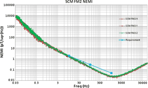
SCM FM2 NEMI measurements. SCM sensitivity requirements are superposed in blue

Table 3 All SCM NEMI at 10 Hz, 100 Hz, 1 kHz. Note that FM1 NEMI is not corrected from the gain error introduced by the original facility

5.5 DFG/AFG/SCM Interference Testing

The respective locations of the three magnetometers onboard MMS satellites have been determined from two interference testing campaigns performed in the amagnetic chamber of the French magnetic observatory of Chambon-la-Forêt. The first one on November 2006 was performed by DFG and SCM teams in order to estimate the possible perturbations of DFG electronics on SCM. SCM noise measurements have been performed for different distances between DFG and SCM sensors; the DFG preamplifier was installed outside the amagnetic chamber. The minimum distance for which the level of perturbations generated by DFG (in the high range gain ±8000 nT) was below the SCM sensitivity was estimated to be 2 m. Possible disturbance on the DFG measurements induced by the SCM ferromagnetic core were also assessed and described in a companion paper by the DFG team (Russell et al. 2014). Briefly, remnant magnetic fields of the SCM core can modify the offset of DFG and the magnetic core can also change the scale factor of the DFG sensor. Both effects were found to be negligible with a distance of 1 m between the two sensors.

The second campaign was held on January 2008 with AFG and SCM teams still using the amagnetic chamber. It aimed to estimate the perturbations on SCM generated by AFG due to its excitation current flowing through its cables. Again, the minimum distance between SCM sensor and AFG cables for which the generated perturbations were below the SCM sensitivity was determined. Assuming a Bessel filter of 5th order, it was concluded that a distance between the AFG cables and the SCM sensor of about 7 cm (or 5 cm with a 6th order filter) left the SCM sensitivity unchanged. The minimum distance between AFG and SCM sensors was also determined. It was established that a separation of about 1 m was sufficient to ensure a nominal functioning for both instruments.

Following these two testing campaigns, the Fields team proposed the MMS configuration described in Sect. 4 with AFG and SCM mounted on the same 5 m magnetometer boom, AFG being at the tip, SCM 4 m from the s/c body and DFG at the tip of the opposite 5 m magnetometer boom.

6 SCM Operational Modes, Data Products and On-Board Calibration

6.1 Operational Modes and Data Products

Different SCM operational modes will depend on the orbit and on the magnetospheric regions. Basically, the orbit, which lasts about 24 hours in Phase 1 and 68 hours in Phase 2, is divided in two parts: slow survey and fast survey periods covering the perigee region and the region of interest respectively. In the slow survey mode (scs), SCM data are sampled at 8 samples per second (S/s) and at 32 S/s in fast survey mode (scf). During the fast survey mode period i.e. inside the region of interest, burst (scb) and high-burst (schb) mode can be triggered thanks to the Burst Trigger Scheme described in Torbert et al. (2014). The sample frequency during the burst mode is 1024 S/s (resp. 8192 S/s) in the dayside (resp. nightside) region. The high-burst mode is always sampled at 16384 S/s whatever the magnetospheric region. Level 2 SCM data products correspond to calibrated SCM data in GSE frame. They are summarized in Table 4. Note that onboard SCM FFT spectra are generated by DSP and described by Torbert et al. (2014).

Table 4 SCM level 2 data products

6.2 On-Board Calibration

The SCM calibration is executed once per orbit shortly after the transition from slow to fast survey. The calibration signal sweep, delivered by DSP, is broken into 4 segments with increasing sample frequencies and the whole calibration sequence lasts less than 90 sec. The frequency of the calibration signal doubles every 4 cycles from 0.125 Hz to 4096 Hz. Each segment will consist of four different frequencies as shown in Table 5. Then the calibration signal is injected into the SCM secondary winding as explained in the previous section. The input voltage can be fixed at four different values (peak-to-peak value): 1.25 V, 2.5 V, 5 V (default value), and 10 V. On the ground, data recorded during on-board SCM calibration sequence will allow us to rebuild the SCM transfer function (gain and phase shift) of the calibration circuit and to track any modifications of the initial SCM transfer function. Then assuming that variations of the calibration circuit transfer function are proportional to the SCM transfer function, the latter can be corrected for. Time domain as well as Fourier domain methods have been developed. Both techniques give good results. The former method is based on convolution of the output signal with a sinusoid for each 4 cycles at one frequency as shown in Fig. 12. The latter method consist of calculating the complex Fourier transform of both input and output signals for each segment then getting the ratio of the spectral densities and the phase difference of the two complex spectra. Results are plotted in Fig. 13.

Fig. 12

From the top: example of X, Y and Z waveforms of input (red, divided by a factor 5 to be plotted in the same scale), output (black) and estimated (blue) calibration signals for the 2nd segment (2, 4, 8, 16 Hz), estimated gain and phase shift of the three channels superposed with Chambon gain and phase shift (dashed line) measurements. Discrepancies at high frequency appear as the calibration signal frequency gets closer to the sample frequency

Fig. 13

From the top: example of X, Y and Z waveforms of input (red) and output (black) calibration signals for the 2nd segment (2, 4, 8, 16 Hz), corresponding complex Fourier spectra (X: black, Y: green, Z: red) and estimated gain and phase shift of the three channels superposed with Chambon gain (dotted line) and phase shift (dashed line) measurements. Discrepancies at high frequency appear as the calibration signal frequency gets closer to the sample frequency

Table 5 Characteristics of the four segments of the on-board calibration signal generated by the DSP

7 Conclusion

The SCM instrument measures the 3D magnetic field fluctuations in the 1 Hz–6 kHz nominal frequency range. The tri-axis system of magnetic antennas is very compact (100 mm³) and light (∼214 g). It is connected to a low noise and low power consumption (∼130 mW) preamplifier built in a robust 3D PLUS technology and the total SCM mass (sensor+preamplifier) is about 420 g. Its sensitivity is less or equal than $2~\mbox{pT/}\sqrt{\mbox{(Hz)}}$ at 10 Hz, $0.18~\mbox{pT/}\sqrt{\mbox{(Hz)}}$ at 100 Hz and $0.025~\mbox{pT/}\sqrt{\mbox{(Hz)}}$ at 1 kHz and is therefore fully compliant with the MMS requirement. With electric field measurements provided by the SDP and ADP instruments, the SCM instrument will allow characterization of the electromagnetic field fluctuations which are expected to play a crucial role in many different physical processes in the collisionless magnetospheric plasma. Thanks to the on-board calibration signal delivered by the DSP once per orbit on each s/c, any possible modifications of the SCM transfer function shall be identified and compensated during the mission. Such verifications are particularly important for very precise multisatellite analysis based on the measurements of amplitude and/or phase of the magnetic fluctuations on board of the four MMS spacecraft.

Appendices

Appendix A: Analytical SCM Transfer Function

The analytical transfer function results from the combination of the transfer function of the feedback flux amplifier given by (7) and the transmittances of the filtering. First of all, by considering the low-pass filtering behavior of the first stage preamplifier of gain G ₁, we obtain:

$$ T(j\omega)=\frac{V_{out}}{B} = \frac{-j \omega N \mu_{app} S \frac {G_1}{1+ j \omega/\omega_{G_1}}}{(1-\mathit{LC}\omega^2)+j(RC\omega+ \frac {G_1}{1+ j \omega/\omega_{G_1}}M/R_{fb})} $$

(8)

Then, low frequencies are filtered out by a high-pass filter given by:

$$ T_{hp}(j\omega) = \frac{-j \omega/\omega_{hp}}{1+ j \omega/\omega_{hp}} $$

(9)

And finally, the signal is amplified by the second stage of the preamplifier (G ₂) and the high frequencies are also filtered out by the following filter:

$$ T_{lp}(j\omega) = \frac{-j \omega/\omega_{lp}G_2}{1+ j \omega/\omega_{lp}} $$

(10)

The total transfer function will be obtained by combining the three transfer functions:

$$ T_{tot}(j\omega) = T(j\omega)T_{hp}(j\omega)T_{lp}(j \omega) $$

(11)

Next, the theoretical transfer function is computed and compared to the measured one at Chambon-la-Forêt observatory (cf. Sect. 5.3). The comparison displayed in Fig. 14 between the measured and calculated transfer functions is rather good. Some disturbances around 50 Hz, corresponding to the power supply line in France, are visible on the measured transfer function. The use of the theoretical transfer function permits to remove it and also to smooth the low-frequency part of the TF which is very sensitive to disturbances.

Fig. 14

FM4 transfer function for X-axis: measured versus modeled

Appendix B: Internal SCM Noise Sources

The total SCM output noise depends on the different noise source contributions in the full frequency range (Coillot and Leroy 2012). At low frequency (i.e. $\omega\ll1/\sqrt{\mathit{LC}}$), the spectral density of the output noise PSD _out can be expressed:

$$ \mathit{PSD}_{out} (f) = (G_1 \times G_2)^2 \bigl(4kTR+e_{PA}^2 + \bigl(Zi_{PA}^2 \bigr) \bigr) $$

(12)

where G ₁ and G ₂ are respectively the gains of first and second stages of the preamplifier, T is the temperature, k the Boltzmann constant, R the resistance of the primary coil of the antenna, Z the antenna impedance, e _PA and i _PA the preamplifier input voltage and current respectively. Since the current noise is rather small (${<}100~\mbox{fA/}\sqrt{\mbox{Hz}}$) the last term can be neglected and the previous equation becomes:

$$ \mathit{PSD}_{out} (f) = (G_1 \times G_2)^2 \bigl(4kTR+e_{PA}^2 \bigr) $$

(13)

Using the SCM design parameters, we can get an estimation of the output voltage noise at low frequency ($\sqrt{\mathit{PSD}_{out}}$) about: . Then, the quantization which permits to convert the analog signal into a digital one must be suited to the output noise. This quantization should permit the study of natural wave spectrum at level comparable to the noise floor of the magnetometer. For this purpose, the low significant bit (LSB) of the analog-to-digital converter (ADC) should be determined in such a way that the r.m.s value of the output noise should be sufficient to cause a bit change at each sampling step with a high probability.

In other words, at each sampling, the probability p of bit change defined by

$$ p(-\mathit{LSB}/2< x<\mathit{LSB}/2)=\int_{-\mathit{LSB}/2} ^{\mathit{LSB}/2} f(x) dx $$

(14)

should be as close as possible to 1. In this expression, f(x) is a Gaussian law which is typical of white noise (while low frequency noise is neglected in this approach) and writes $f(x) = 1 \backslash(\sigma\sqrt{2 \pi}) \exp(-x^{2} \backslash(2 \sigma^{2}))$. The standard-deviation σ of the Gaussian law is equivalent to the r.m.s value of the noise V _n determined by:

$$ \sigma= V_n = \sqrt{ \int_0 ^{F_{max}} \mathit{PSD}_{out} (f) df} \simeq\sqrt {\mathit{PSD}_{out}(f) \times F_{max} } $$

(15)

where F _max represents the maximum frequency of the analog electronic conditioner. In practice, the integration can be limited to the bandwidth of the preamplifier (i.e. the cutoff frequency of the second stage, namely: F _max =f _lp ), especially because of the aliasing filtering which will cut strongly the noise outside the frequency band. Practically, to digitize the noise with a probability sufficiently high (close to 0.9) to be able to keep the noise fluctuations, the digitization should verify

$$ \frac{\mathit{LSB}}{2} \leq V_n $$

(16)

Under this consideration and assuming a white noise over the full frequency band (while in practice the noise could be slightly reduced in the frequency range where the transfer function flattened depending on R _fb value), the estimated value of the output r.m.s voltage noise is approximately V _n =12 mV. However, the amplifier output is scaled to the ADC using a 6 dB attenuator, the RMS noise value becomes V _n =6 mV. On the other hand, the digitization of SCM is done using 16 bits over a dynamic range of ±2.5 V. Thus, the LSB value is 76∼μV and condition given by (16) is amply verified.

References

L. Andersson, R.E. Ergun, J. Tao, A. Roux, O. Lecontel, V. Angelopoulos, J. Bonnell, J.P. McFadden, D.E. Larson, S. Eriksson, T. Johansson, C.M. Cully, D.N. Newman, M.V. Goldman, K.-H. Glassmeier, W. Baumjohann, New features of electron phase space holes observed by the THEMIS mission. Phys. Rev. Lett. 102(22), 225004 (2009). doi:10.1103/PhysRevLett.102.225004
D. Attié, L. Rezeau, G. Belmont, N. Cornilleau-Wehrlin, E. Lucek, Power of magnetopause low-frequency waves: a statistical study. J. Geophys. Res. 113, 7213 (2008). doi:10.1029/2007JA012606
S.D. Bale, F.S. Mozer, T. Phan, Observation of lower hybrid drift instability in the diffusion region at a reconnecting magnetopause. Geophys. Res. Lett. 29, 2180 (2002). doi:10.1029/2002GL016113
J. Birn, J.F. Drake, M.A. Shay, B.N. Rogers, R.E. Denton, M. Hesse, M. Kuznetsova, Z.W. Ma, A. Battacharjee, A. Otto, P.L. Pritchett, Geospace environmental modeling (GEM) magnetic reconnection challenge. J. Geophys. Res. 106, 3715–3719 (2001)
J. Burch, The MMS mission. Space Sci. Rev. (2014), this issue
C.A. Cattell, F.S. Mozer, in Substorm-Associated Lower Hybrid Waves in the Plasma Sheet Observed by ISEE 1, ed. by A.T.Y. Lui, S.-I. Akasofu (1987), pp. 119–125
C. Cattell, J. Wygant, F.S. Mozer, T. Okada, K. Tsuruda, S. Kokubun, T. Yamamoto, ISEE 1 and Geotail observations of low-frequency waves at the magnetopause. J. Geophys. Res. 100, 11823 (1995). doi:10.1029/94JA03146
C. Cattell, J. Dombeck, J. Wygant, J.F. Drake, M. Swisdak, M.L. Goldstein, W. Keith, A. Fazakerley, M. André, E. Lucek, A. Balogh, Cluster observations of electron holes in association with magnetotail reconnection and comparison to simulations. J. Geophys. Res. 110, 1211 (2005). doi:10.1029/2004JA010519
C.C. Chaston, J.W. Bonnell, L. Clausen, V. Angelopoulos, Energy transport by kinetic-scale electromagnetic waves in fast plasma sheet flows. J. Geophys. Res. 117, 9202 (2012). doi:10.1029/2012JA017863
C. Chaston, J. Bonnell, J.P. McFadden, C.W. Carlson, C. Cully, O. Le Contel, A. Roux, H.U. Auster, K.H. Glassmeier, V. Angelopoulos, C.T. Russell, Turbulent heating and cross-field transport near the magnetopause from THEMIS. Geophys. Res. Lett. 35, 17 (2008). doi:10.1029/2008GL033601
L. Chen, A. Hasegawa, Kinetic theory of geomagnetic pulsations, 1, internal excitations by energetic particles. J. Geophys. Res. 96, 1503 (1991)
C. Coillot, P. Leroy, in Induction Magnetometers Principle, Modeling and Ways of Improvement, ed. by K. Huang (2012)
C. Coillot, J. Moutoussamy, P. Leroy, G. Chanteur, A. Roux, Improvements on the design of search coil magnetometer for space experiments. Sens. Lett. 5, 1–4 (2007)
N. Cornilleau-Wehrlin, P. Chauveau, S. Louis, A. Meyer, J.M. Nappa, S. Perraut, L. Rezeau, P. Robert, A. Roux, C. de Villedary, Y. de Conchy, L. Friel, C.C. Harvey, D. Hubert, C. Lacombe, R. Manning, F. Wouters, F. Lefeuvre, M. Parrot, J.-L. Pinçon, B. Poirier, W. Kofman, P. Louarn, The Cluster spatio-temporal analysis of field fluctuations (STAFF) experiment. Space Sci. Rev. 79, 107–136 (1997)
N. Cornilleau-Wehrlin, G. Chanteur, S. Perraut, L. Rezeau, P. Robert, A. Roux, C. de Villedary, P. Canu, M. Maksimovic, Y. de Conchy, D. Hubert, C. Lacombe, F. Lefeuvre, M. Parrot, J.-L. Pinçon, P.M.E. Décréau, C.C. Harvey, P. Louarn, O. Santolik, H. St. Alleyne, M. Roth, T. Chust, O. Le Contel, S. team, First results obtained by the Cluster STAFF experiment. Ann. Geophys. 21, 437–456 (2003)
W. Daughton, The unstable eigenmode of a neutral sheet. Phys. Plasmas 6(4), 1329–1343 (1999)
J.F. Drake, M.A. Shay, M. Swisdak, The Hall fields and fast magnetic reconnection. Phys. Plasmas 15, 042306 (2008)
R.E. Ergun, J. Westfall, S. Tucker, The axial double probe sensors and fields signal processing for the MMS mission. Space Sci. Rev. (2014), this issue
R.E. Ergun, L. Andersson, J. Tao, V. Angelopoulos, J. Bonnell, J.P. McFadden, D.E. Larson, S. Eriksson, T. Johansson, C.M. Cully, D.N. Newman, M.V. Goldman, A. Roux, O. Lecontel, K.-H. Glassmeier, W. Baumjohann, Observations of double layers in Earth’s plasma sheet. Phys. Rev. Lett. 102(15), 155002 (2009). doi:10.1103/PhysRevLett.102.155002
G. Fruit, P. Louarn, A. Tur, Electrostatic “bounce” instability in a magnetotail configuration. Phys. Plasmas 20(2), 022113 (2013). doi:10.1063/1.4793442
R. Gendrin, Magnetic turbulence and diffusion processes in the magnetopause boundary layer. Geophys. Res. Lett. 10, 769–771 (1983). doi:10.1029/GL010i008p00769
D.A. Gurnett, L.A. Frank, R.P. Lepping, Plasma waves in the distant magnetotail. J. Geophys. Res. 81, 6059–6071 (1976)
D.A. Gurnett, R.R. Anderson, B.T. Tsurutani, E.J. Smith, G. Paschmann, G. Haerendel, S.J. Bame, C.T. Russell, Plasma wave turbulence at the magnetopause—observations from ISEE 1 and 2. J. Geophys. Res. 84, 7043–7058 (1979). doi:10.1029/JA084iA12p07043
D.A. Gurnett, W.S. Kurth, D.L. Kirchner, G.B. Hospodarsky, T.F. Averkamp, P. Zarka, A. Lecacheux, R. Manning, A. Roux, P. Canu, N. Cornilleau-Wehrlin, P. Galopeau, A. Meyer, R. Boström, G. Gustafsson, J.-E. Wahlund, L. Åhlén, H.O. Rucker, H.P. Ladreiter, W. Macher, L.J.C. Woolliscroft, H. Alleyne, M.L. Kaiser, M.D. Desch, W.M. Farrell, C.C. Harvey, P. Louarn, P.J. Kellogg, K. Goetz, A. Pedersen, The Cassini radio and plasmawave investigation. Space Sci. Rev. 114, 395–463 (2004)
H. Hasegawa, M. Fujimoto, T.-D. Phan, H. Rème, A. Balogh, M.W. Dunlop, C. Hashimoto, R. TanDokoro, Transport of solar wind into Earth’s magnetosphere through rolled-up kelvin–Helmholtz vortices. Nature 430, 755–758 (2004). doi:10.1038/nature02799
M. Hesse, K. Schindler, J. Birn, M. Kuznetsova, The diffusion region in collisionless magnetic reconnection. Phys. Plasmas 6, 1781–1795 (1999). doi:10.1063/1.873436
J.D. Huba, N.T. Gladd, K. Papadopoulos, The lower-hybrid-drift instability as a source of anomalous resistivity for magnetic field line reconnection. Geophys. Res. Lett. 4, 125–128 (1977). doi:10.1029/GL004i003p00125
O.A. Hurricane, R. Pellat, F.V. Coroniti, A new approach to low-frequency “MHD-like” waves in magnetospheric plasmas. J. Geophys. Res. 100, 19421 (1995)
Y. Kasaba, J.-L. Bougeret, L.G. Blomberg, H. Kojima, S. Yagitani, M. Moncuquet, J.-G. Trotignon, G. Chanteur, A. Kumamoto, Y. Kasahara, J. Lichtenberger, Y. Omura, K. Ishisaka, H. Matsumoto, The plasma wave investigation (PWI) onboard the BepiColombo/MMO: first measurement of electric fields, electromagnetic waves, and radio waves around Mercury. Planet. Space Sci. 58, 238–278 (2010). doi:10.1016/j.pss.2008.07.017
C.F. Kennel, F.V. Coroniti, F.L. Scarf, Plasma waves in magnetotail flux ropes. J. Geophys. Res. 91, 1424–1438 (1986)
Y.V. Khotyaintsev, C.M. Cully, A. Vaivads, M. André, C.J. Owen, Plasma jet braking: energy dissipation and nonadiabatic electrons. Phys. Rev. Lett. 106(16), 165001 (2011). doi:10.1103/PhysRevLett.106.165001
O. Le Contel, R. Pellat, A. Roux, Self-consistent quasi-static radial transport during the substorm growth phase. J. Geophys. Res. 105, 12929–12944 (2000)
O. Le Contel, A. Roux, S. Perraut, R. Pellat, Ø. Holter, A. Pedersen, A. Korth, Possible control of plasma transport in the near-Earth plasma sheet via current-driven Alfvén waves (f≃f H+) during substorm growth phase and relation to breakup. J. Geophys. Res. 106, 10817–10827 (2001)
O. Le Contel, A. Roux, P. Robert, C. Coillot, A. Bouabdellah, B. de la Porte, D. Alison, S. Ruocco, V. Angelopoulos, K. Bromund, C.C. Chaston, C. Cully, First results of THEMIS Search Coil Magnetometers (SCM). Space Sci. Rev. (2008). doi:10.1007/s11214-008-9371-y
O. Le Contel, A. Roux, C. Jacquey, P. Robert, M. Berthomier, T. Chust, B. Grison, V. Angelopoulos, D. Sibeck, C.C. Chaston, C.M. Cully, B. Ergun, K.-H. Glassmeier, U. Auster, J. McFadden, C. Carlson, D. Larson, J.W. Bonnell, S. Mende, C.T. Russell, E. Donovan, I. Mann, H. Singer, Quasi-parallel whistler mode waves observed by THEMIS during near-earth dipolarizations. Ann. Geophys. 27, 2259–2275 (2009). doi:10.5194/angeo-27-2259-2009
J. Lemaire, Impulsive penetration of filamentary plasma elements into the magnetospheres of the Earth and Jupiter. Planet. Space Sci. 25, 887–890 (1977). doi:10.1016/0032-0633(77)90042-3
P.A. Lindquist, G. Olson, R. Torbert, B. King, Y. Khotyaintsev, A. Eriksson, L. Åhlén, Porter, R.E. Ergun, The spin-plane double probe instrument for MMS. Space Sci. Rev. (2014), this issue
A.T. Lui, R.E. Lopez, B.J. Anderson, K. Takahashi, L.J. Zanetti, R.W. McEntire, T.A. Potemra, D.M. Klumpar, E.M. Greene, R. Strangeway, Current disruption in Earth’s magnetosphere: observations and models. J. Geophys. Res. 101, 13067–13088 (1996)
M.E. Mandt, R.E. Denton, J.F. Drake, Transition to whistler mediated magnetic reconnection. Geophys. Res. Lett. 21(1), 73–77 (1994)
J.D. Means, Use of the three-dimensional covariance matrix in analyzing the polarization properties of plane waves. J. Geophys. Res. 77, 5551–5559 (1972)
T.G. Northrop, E. Teller, Stability of the adiabatic motion of charged particles in the Earth’s field. Phys. Rev. 117, 215–225 (1960). doi:10.1103/PhysRev.117.215
J.A. Osborn, Demagnetizing factors of the general ellipsoid. Phys. Rev. 67(11–12), 351–357 (1945)
G.K. Parks, E. Lee, N. Lin, F. Mozer, M. Wilber, I. Dandouras, H. Rème, E. Lucek, A. Fazakerley, M. Goldstein, C. Gurgiolo, P. Canu, N. Cornilleau-Wehrlin, P. Décréau, Solitary electromagnetic pulses detected with super-Alfvénic flows in Earth’s geomagnetic tail. Phys. Rev. Lett. 98(26), 265001 (2007). doi:10.1103/PhysRevLett.98.265001
R. Pellat, O.A. Hurricane, F.V. Coroniti, Multipole stability revisited. Phys. Plasmas 1, 3502 (1994)
S. Perraut, R. Gendrin, P. Robert, A. Roux, Magnetic pulsations observed on board GEOS-2 in the ULF range during multiple magnetopause crossings, in Magnetospheric Boundary Layers, ed. by B. Battrick, J. Mort, G. Haerendel, J. Ortner. ESA Special Publication, vol. 148 (1979), pp. 113–122
T.D. Phan, C.P. Escoubet, L. Rezeau, R.A. Treumann, A. Vaivads, G. Paschmann, S.A. Fuselier, D. Attié, B. Rogers, B.U.Ö. Sonnerup, Magnetopause processes. Space Sci. Rev. 118, 367–424 (2005). doi:10.1007/s11214-005-3836-z
J.L. Pinçon, F. Lefeuvre, Local characterization of homogeneous turbulence in a space plasma from simultaneous measurements of field components at several points in space. J. Geophys. Res. 96, 1789–1802 (1991). doi:10.1029/90JA02183
J.L. Pinçon, F. Lefeuvre, The application of the generalized Capon method to the analysis of a turbulent field in space plasma—experimental constraints. J. Atmos. Terr. Phys. 54, 1237–1247 (1992)
P.L. Pritchett, F.V. Coroniti, Three-dimensional collisionless magnetic reconnection in the presence of a guide field. J. Geophys. Res. 109, 1220 (2004). doi:10.1029/2003JA009999
L. Rezeau, S. Perraut, A. Roux, Electromagnetic fluctuations in the vicinity of the magnetopause. Geophys. Res. Lett. 13, 1093–1096 (1986). doi:10.1029/GL013i011p01093
L. Rezeau, A. Morane, S. Perraut, A. Roux, R. Schmidt, Characterization of Alfvenic fluctuations in the magnetopause boundary layer. J. Geophys. Res. 94, 101–110 (1989). doi:10.1029/JA094iA01p00101
J.G. Roederer, On the adiabatic motion of energetic particules in a model magnetosphere. J. Geophys. Res. 77, 624 (1967)
B.N. Rogers, R.E. Denton, J.F. Drake, M.A. Shay, Role of dispersive waves in collisionless magnetic reconnection. Phys. Rev. Lett. 87(19), 195004 (2001). doi:10.1103/PhysRevLett.87.195004
A. Roux, O. Le Contel, P. Robert, C. Coillot, A. Bouabdellah, B.d. la Porte, D. Alison, S. Ruocco, M.C. Vassal, The search coil magnetometer (SCM) for THEMIS. Space Sci. Rev. 141, 265 (2009)
A. Roux, P. Robert, O. Le Contel, V. Angelopoulos, U. Auster, J. Bonnell, C.M. Cully, R.E. Ergun, J.P. McFadden, A mechanism for heating electrons in the magnetopause current layer and adjacent regions. Ann. Geophys. 29, 2305–2316 (2011). doi:10.5194/angeo-29-2305-2011
C.T. Russell, B. Anderson, W. Baumjohann, K. Bromund, D. Dearborn, G. Le, H. Leinweber, D. Leneman, W. Magnes, J.D. Means, M. Moldwin, R. Nakamura, D. Pierce, K. Rowe, J.A. Slavin, R.J. Strangeway, The magnetospheric multiscale magnetometers. Space Sci. Rev. (2014), this issue. doi:10.1007/s11214-014-0057-3
F. Sahraoui, J.-L. Pinçon, G. Belmont, L. Rezeau, N. Cornilleau-Wehrlin, P. Robert, L. Mellul, J.-M. Bosqued, A. Balogh, P. Canu, G. Chanteur, ULF wave identification in the magnetosheath: the k-filtering technique applied to Cluster II data. J. Geophys. Res. 108, 1335 (2003). doi:10.1029/2002JA009587
J.C. Samson, J.V. Olson, Some comments on the descriptions of the polarization states of waves. Geophys. J. R. Astron. Soc. 61, 115–129 (1980)
N. Sckopke, G. Paschmann, G. Haerendel, B.U.O. Sonnerup, S.J. Bame, T.G. Forbes, E.W. Hones Jr., C.T. Russell, Structure of the low latitude boundary layer, Technical report (1981)
I. Shinohara, T. Nagai, M. Fujimoto, T. Terasawa, T. Mikai, K. Tsuruda, T. Yamamoto, Low-frequency electromagnetic turbulence observed near the substorm onset site. J. Geophys. Res. 103, 20365 (1998)
D.G. Sibeck, A model for the transient magnetospheric response to sudden solar wind dynamic pressure variations. J. Geophys. Res. 95, 3755–3771 (1990). doi:10.1029/JA095iA04p03755
R. Smets, G. Belmont, D. Delcourt, L. Rezeau, Diffusion at the Earth magnetopause: enhancement by Kelvin–Helmholtz instability. Ann. Geophys. 25, 271–282 (2007). doi:10.5194/angeo-25-271-2007
G. Stenberg, T. Oscarsson, M. André, A. Vaivads, M. Morooka, N. Cornilleau-Wehrlin, A. Fazakerley, B. Lavraud, P.M.E. Décréau, Electron-scale sheets of whistlers close to the magnetopause. Ann. Geophys. 23, 3715–3725 (2005)
J.B. Tao, R.E. Ergun, L. Andersson, J.W. Bonnell, A. Roux, O. LeContel, V. Angelopoulos, J.P. McFadden, D.E. Larson, C.M. Cully, H.-U. Auster, K.-H. Glassmeier, W. Baumjohann, D.L. Newman, M.V. Goldman, A model of electromagnetic electron phase-space holes and its application. J. Geophys. Res. 116, 11213 (2011). doi:10.1029/2010JA016054
A. Tenerani, O. Le Contel, F. Califano, F. Pegoraro, P. Robert, N. Cornilleau-Wehrlin, J.A. Sauvaud, Coupling between Whistler waves and ion-scale solitary waves: Cluster measurements in the magnetotail during a substorm. Phys. Rev. Lett. 109(15), 155005 (2012). doi:10.1103/PhysRevLett.109.155005
A. Tenerani, O. Le Contel, F. Califano, P. Robert, D. Fontaine, N. Cornilleau-Wehrlin, J.A. Sauvaud, Cluster observations of whistler waves correlated with ion-scale magnetic structures during the August 17th 2003 substorm event. J. Geophys. Res. 118, 1–18 (2013). doi:10.1002/jgra.50562
R.B. Torbert, C.T. Russell, W. Magnes, R.E. Ergun, P.-A. Lindqvist, O.L. Contel, H. Vaith, J. Macri, S. Myers, D. Rau, J. Needell, B. King, M. Granoff, M. Chutter, I. Dors, G. Olsson, Y. Khotyaintsev, A. Eriksson, C.A. Kletzing, S. Bounds, B. Anderson, W. Baumjohann, M. Steller, K. Bromund, G. Le, R. Nakamura, R.J. Strangeway, S. Tucker, J. Westfall, D. Fischer, F. Plaschke, The FIELDS instrument suite on MMS: scientific objectives, measurements, and data products. Space Sci. Rev. (2014), this issue
B.T. Tsurutani, R.M. Thorne, Diffusion processes in the magnetopause boundary layer. Geophys. Res. Lett. 9, 1247–1250 (1982). doi:10.1029/GL009i011p01247
S. Tumanski, Induction coil sensors—a review. Meas. Sci. Technol. 18, 31 (2007). doi:10.1088/0957-0233/18/3/R01
A. Tur, P. Louarn, V. Yanovsky, Kinetic theory of electrostatic “bounce” modes in two-dimensional current sheets. Phys. Plasmas 17(10), 102905 (2010). doi:10.1063/1.3491423
H. Vaith, R.B. Torbert, M. Granoff, W. Baumjohann, M. Steller, R. Nakamura, F. Plaschke, The EDI instrument for MMS. Space Sci. Rev. (2014), this issue
A. Vaivads, M. André, S.C. Buchert, J.-E. Wahlund, A.N. Fazakerley, N. Cornilleau-Wehrlin, Cluster observations of lower hybrid turbulence within thin layers at the magnetopause. Geophys. Res. Lett. 31, 3804 (2004). doi:10.1029/2003GL018142
X.H. Wei, J.B. Cao, G.C. Zhou, O. Santolík, H. Rème, I. Dandouras, N. Cornilleau-Wehrlin, E. Lucek, C.M. Carr, A. Fazakerley, Cluster observations of waves in the Whistler frequency range associated with magnetic reconnection in the Earth’s magnetotail. J. Geophys. Res. 112, 10225 (2007). doi:10.1029/2006JA011771
J. Weiland, in Collective Modes in Inhomogeneous Plasma, ed. by P. Stott, H. Wilhelmsson (Institute of Physics, Bristol, 2000)
Y. Zhang, H. Matsumoto, H. Kojima, Whistler mode waves in the magnetotail. J. Geophys. Res. 104, 28633–28644 (1999)
Acknowledgements
The French participation in the MMS mission is supported by CNES and CNRS-INSU. The SCM documentation (product assurance) for each FM has been established with the support of the Nexeya company via a contract funded by CNRS-INSU/CNES. We are pleased to acknowledge the friendly collaboration and the help of our American colleagues from UNH and LASP, from SWRI and GSFC as well as of our European colleagues from KTH, IRFU, IWF and TUBS. We thank also B. Dufour, M. Beaudier, X. Lalane, K. Telali, B. Heumez, E. Parmentier from IPGP for their support during the building and using of the new facility at Chambon-la-Forêt.
Author information
Authors and Affiliations
Corresponding author