
Abstract
NASA’s InSight Mission will deploy two three-component seismometers on Mars in 2018. These short period and very broadband seismometers will be mounted on a three-legged levelling system, which will sit directly on the sandy regolith some 2–3 meters from the lander. Although the deployment will be covered by a wind and thermal shield, atmospheric noise is still expected to couple to the seismometers through the regolith. Seismic activity on Mars is expected to be significantly lower than on Earth, so a characterisation of the extent of coupling to noise and seismic signals is an important step towards maximising scientific return.
In this study, we conduct field testing on a simplified model of the seismometer assembly. We constrain the transfer function between the wind and thermal shield and tripod-mounted seismometers over a range of frequencies (1–40 Hz) relevant to the deployment on Mars. At 1–20 Hz the displacement amplitude ratio is approximately constant, with a value that depends on the site (0.03–0.06). The value of the ratio in this range is 25–50% of the value expected from the deformation of a homogeneous isotropic elastic halfspace. At 20–40 Hz, the ratio increases as a result of resonance between the tripod mass and regolith. We predict that mounting the InSight instruments on a tripod will not adversely affect the recorded amplitudes of vertical seismic energy, although particle motions will be more complex than observed in recordings generated by more conventional buried deployments. Higher frequency signals will be amplified by tripod-regolith resonance, probably reaching peak-amplification at \(\sim 50\) Hz. The tripod deployment will lose sensitivity at frequencies \(>50\) Hz as a result of the tripod mass and compliant regolith.
We also investigate the attenuation of seismic energy within the shallow regolith covering the range of seismometer deployment distances. The amplitude of surface displacement decays as \(r^{-n}\), where \(1.5 < n < 2\). This exceeds the value expected for a homogeneous isotropic elastic halfspace (\(n \sim 1\)), and reflects an increase in Young’s modulus with depth. We present an updated model of lander noise which takes this enhanced attenuation into account.
1 Introduction
NASA’s Interior Exploration using Seismic Investigations, Geodesy and Heat Transport (InSight; Banerdt et al. 2012) mission was launched in May 2018, and will land on Mars in November 2018. It will be the first mission to deploy seismometers on Mars since Viking 1 and 2, which landed in 1976 (Anderson et al. 1976; Flinn 1977; Lazarewicz et al. 1981). InSight will deploy three-component short-period (SP; Pike et al. 2005; Delahunty and Pike 2014) and very broad-band (VBB; Dandonneau et al. 2013; Lognonne et al. 2014) seismometers, which together comprise the instruments for the Seismic Experiment for Interior Structure (SEIS; Mimoun et al. 2012). This experiment is designed to provide the first detailed constraints on the structure of the planet, including properties of the crust (Panning et al. 2015, 2017), deep interior (Khan et al. 2016) and the radius and mass of the core (Hempel et al. 2016). Unlike the lander-mounted seismometers of the Viking Mission, the instruments will be mounted on a levelling system consisting of three linear-actuator legs on a frame (LVL; Mimoun et al. 2017), which will be transferred from the lander onto the surface of Mars (Fig. 1).

The deployment sequence for the seismic instruments on-board the InSight lander. (a) The scientific instruments are mounted on the lander deck. (b) The LVL with SP/VBB seismometers are deployed to the surface by a robot arm. (c) The robot arm positions the WTS over the SEIS instruments. (d) The WTS is lowered to the ground surface. The legs of the LVL and WTS are not shown in (a)–(d). (e) Schematic of the SEIS experiment with inner (LVL) tripod and outer (WTS) tripod. The WTS has a flexible chainmail skirt to help isolate the SEIS experiment from wind and thermal variations. Images (a)–(d) courtesy of NASA/JPL-Caltech
Seismic sources recorded by the InSight Mission are expected to have two primary origins: meteorite impacts and airbursts (Davis 1993; Teanby and Wookey 2011; Teanby 2015; Stevanović et al. 2017), and faulting as a response to stress generated by uncompensated gravitational loads, igneous intrusions and cooling of the planet (Phillips and Grimm 1991; Golombek et al. 1992; Knapmeyer et al. 2006; Taylor et al. 2013). Faulting has occurred on Mars within the last few million years (Taylor et al. 2013), and there are intriguing suggestions that some regions are seismically active at the present day (Roberts et al. 2012). Sources of seismicity are reviewed by Panning et al. (2017), and so we only mention a few key points here. The majority of faults on Mars’ surface are associated with volcanic activity or gravitational collapse around Tharsis (to a distance of \(>90^{\circ }\) from the center of the province), or associated with the many impact basins over Mars’ surface (Knapmeyer et al. 2006). The present day strain rate, the maximum depth of brittle behaviour, and the size distribution of Marsquakes are all poorly known. Strain rates due to cooling will be spatially variable, with high rates expected around large igneous bodies beneath the Tharsis volcanic province. Fault reactivation is likely to be the energetically preferred mechanism to relieve thermal stresses, but the amount of observed slip attributable to thermal contraction is unknown.
Given the uncertainties in the distribution and magnitude of global seismic moment release on Mars, it is vital to optimize the deployment of the SEIS package. Deployment problems hampered attempts to unambiguously identify marsquakes from the Viking Mission data (Lazarewicz et al. 1981); the seismometer on Viking 1 failed to uncage, and one of the legs of Viking 2 rested on a rock, causing tilting of \(8.2 ^{\circ }\) and therefore complicating the response of the instrument to seismic noise. The VBBs chosen for the InSight Mission would not operate at such a large angle of tilt, necessitating the use of the LVL system to allow for ground tilt and small rocks that require some ground clearance of the sensor.
Reduction of atmospheric and thermal noise is also a key requirement of a successful seismometer deployment on Mars. A low atmospheric pressure at the surface (\(\sim 0.7\%\) that at Earth’s surface; Schofield et al. 1997) results in daily temperature variations of \(>80\) K near the equator (Clancy et al. 2000), which generates strong winds in morning and late afternoon. Even with an improved understanding of wind noise, a recent reanalysis of the Viking 2 data resulted in only a single tentative quake identification (Lorenz et al. 2017). To reduce the amount of noise recorded by InSight, the SEIS instruments will be deployed only about 15 cm above the surface of Mars, with a shield protecting the package from wind and thermal fluctuations (WTS; Lognonne et al. 2014). Even with these improvements in design, the number \(N\) events observed during the nominal 2-year mission is estimated to be within the range \(\log _{10}(N) = 1.0\substack{+1.0 \\ -1.5}\) (Panning et al. 2017), where the confidence intervals arise from uncertainties in the estimates of moment release, moment magnitude, seismic attenuation and wind noise. Maximising scientific return from a small number of predicted events necessitates a better understanding of noise (Mimoun et al. 2017) and the response of the SEIS instruments to seismic signals.
In this study, we investigate the effect of mounting the SEIS instruments on the LVL tripod and the attenuation of regolith-transmitted seismic noise. The study builds on two recent studies, also motivated by the InSight Mission. Murdoch et al. (2017) modelled the wind noise expected from motion of the lander, whose large solar panels are expected to be deflected by the wind. They approximated the regolith as a homogeneous elastic half-space, with the lander and SEIS feet as point sources. Teanby et al. (2017) investigated the transfer coefficient between the WTS and SEIS tripods through field experiments at 5 Hz. They showed that the transfer coefficient at this frequency was significantly lower than would be expected for elastic deformation, and suggested that anelastic effects might cause dissipation of the noise.
In this study, we extend the work of Teanby et al. (2017) with further analogue experiments and numerical modelling. Our aims are to:
-
1.
Determine the frequency-dependent displacement amplitude ratio (hereafter transfer coefficient) between the WTS and SEIS tripods.
-
2.
Quantify the attenuation with distance, for application to noise coupling between the lander and SEIS experiment.
-
3.
Investigate the coupling between seismometers and regolith during tripod-mounted deployments relative to more conventional buried deployment.
-
4.
Isolate the cause of discrepancy between experimental observations and elastic model predictions of WTS-SEIS coupling (Teanby et al. 2017).
2 Field Sites
Our field experiments were carried out in northeast Iceland, famed for its cold deserts and commonly used as a Mars analogue (e.g. Greeley et al. 2002; Hartmann et al. 2003). The regolith in these areas is typically sandy and basaltic in composition (Arnalds et al. 2001).
Following the logic of Teanby et al. (2017), the sites in this study were chosen for their good drainage and lack of soil and vegetation. The regolith at all three sites was composed of medium-to-coarse surface sand (median grain size 0.1–1.0 mm) underlain by slightly finer sand. In comparison, the most common regolith within the InSight landing ellipse is believed to consist of cohesionless \(\sim 0.17\) mm sand (Golombek et al. 2017), with small areas of coarser sand with larger clasts similar to the regolith measured by the Spirit Rover in Gusev Crater (Cabrol et al. 2014), and very small areas consisting of non-load-bearing dust.
The first field site is located just north of Hverfell tephra crater (\(65^{\circ }37'35.0''\) N, \(16^{\circ }51'49.2''\) W; Mattsson and Höskuldsson 2011), on thin (0.5–2.0 m) regolith surrounded by basaltic lava flows. The second site is a small basaltic sand quarry north of Fellabær (\(65 ^{\circ }20'49.3''\) N, \(14^{\circ }25'25.4''\) W), with highly compacted ground chosen as a contrast to the other two sites. The third site lies on the edge of basaltic sand dunes in the Héraðsflói area, just north of the F94 about 15 km west of Bakkagerði (\(65 ^{\circ }35'15.2''\) N; \(14^{\circ }07'23.7''\) W). The two latter sites have a regolith several meters thick. Similarly, 85% of the InSight landing site is covered by a regolith that is at least 3 m thick, and may be as thick as 12 to 18 m (Warner et al. 2017). Figure 2 shows the location of all three sites.

Locations and photographs of field sites used in this study
3 Experimental Methods
3.1 WTS and SEIS Tripod Analogues
Our analogues of the WTS and SEIS tripods were constructed from 3 mm thick aluminium angle-sections (Fig. 3). The inner tripod had a side length of 0.30 m and the outer tripod had a side length of 0.80 m. The foot design for the two tripods consists of a 60 mm diameter anti-sink disc surrounding a 19 mm diameter shaft with a \(45 ^{\circ }\) tapered spike. The final design of the InSight feet differs somewhat from this design: the spikes on the SEIS feet are 20 mm long with a top diameter of 10 mm, while the WTS feet consist of a thin triangular blade and some additional roughness on the circular anti-sink disk. These differences will primarily influence horizontal coupling to the regolith (see Discussion).

Experimental apparatus and setup for the different experiments conducted in this study. (a) Experimental setup for the WTS-SEIS transfer coefficient experiments. The spring sources mounted to the outer tripod have oscillatory frequencies of 0.6–40 Hz (the source shown in this figure has a natural frequency of 5.3 Hz). (b) The setup for the ambient noise experiments has one seismometer buried in the regolith so that the top is flush with the surface (just visible under tripod). The tripod-mounted seismometer is aligned relative to the buried seismometer. (c) Setup for the regolith-SEIS coupling experiments. As in (b), one seismometer is buried just beneath the surface, while the other is mounted on the smaller tripod. The large tripod is aligned relative to the inner tripod, and a spring source mounted as in (a). The setup shown corresponds to the 1.5 Hz source. (d) Setup for the regolith attenuation experiments. The spring sources are mounted to the same metal frame used in (a) and (c), which is coupled to the ground via a metal spike. The spring-mass system shown has a natural frequency of 2.2 Hz. One seismometer is buried in the regolith 0.3 m from the spike. The other is mounted on the small tripod. Recordings of the spring-stimulated ground motions are made with the center of the tripod-mounted seismometer placed 1.0, 2.0 and 3.7 m away from the spike
We used Trillium Compact seismometers (TC120-SV1 variant) which have a response flat to velocity from 120 seconds to 100 Hz, a high clip level of 26 mm/s and an operational tilt range of ±2.5∘. The seismometers were mounted at the center of the inner tripod and close to one corner of the outer tripod, with steel masses on the other two corners to balance the mass distribution. The total masses of the outer and inner tripods were 11 kg and 2.9 kg respectively. The planned masses of the WTS and SEIS tripods are 9.5 kg and 8.2 kg, and as such, the weight of the inner tripod in our analogue experiments on Earth (28.5 N) is similar to the weight of the SEIS tripod on Mars (30.4 N for a gravitational acceleration of 3.71 m/s2). The vertical coupling to the regolith should therefore be similar to that on Mars. The weight of the outer tripod is unimportant in our experiments, as its displacement is driven by an active source. Useful quantities from our field experiments and their equivalents for the InSight Mission (Kedar et al. 2017) are given in Table 1.
Seismic signals detected by the two seismometers were recorded on a 6 channel, 24 bit Nanometrics Centaur data logger set to a voltage range of \(\pm 1\) V. Continuous logging was performed by the on-board software. A field laptop powered by a car battery and power inverter was used to check for signal clipping and record the data. Data were logged at 200 Hz so that our highest frequency source (40 Hz) had a frequency lower than the Nyquist frequency.
3.2 Active Sources
To simulate the transmission of seismic energy from the lander or WTS to the SEIS tripod, a set of harmonic oscillators were mounted to a metal frame, which was fixed either to the apex of three aluminium supports on the outer tripod frame, or to a 0.1 m disk welded to the top of a steel spike driven into the ground (Fig. 3). To minimise horizontal noise and ringing, the metal frame was stabilised with a wooden L-frame. The oscillators comprised a mass connected to springs, the details of which can be found in Table 2. Specific details of the different experimental setups shown in Fig. 3 are described with the results of each setup (Sect. 5). The general procedure for each active-source experiment was as follows:
-
Prime the spring source by pulling down on the mass.
-
Release carefully, minimising horizontal motion.
-
Allow the spring to oscillate until the amplitude was \(<50\)% of its original value (see Table 2 for durations for each spring source).
Table 2 Spring-mass systems used as single-frequency sources in our experiments. \(f_{w}\) is the frequency window over which displacement was integrated. \(t\) is the duration chosen for each oscillation experiment. The number of springs \(n\) is given as the number of springs on one side of the mass, multiplied by either one or two (for a one- or two-sided setup) -
Repeat 6 times, rejecting any experiments affected by noise and tripod vibrations.
-
Repeat for each spring-mass system. Example vertical component seismograms for each spring source are shown in Fig. 4.
Fig. 4 
Example vertical component seismograms from the single-frequency spring sources at the Fellabær site, from seismograms recorded by the outer and inner tripods. From top to bottom, signals at 39 Hz, 20.5 Hz, 9 Hz, 5.3 Hz, 2.2 Hz and 1.55 Hz. Left two columns span the duration of each oscillation. Right two columns span 10 periods
-
Disconnect the seismometers from the datalogger/power source, exchange them, and then reconnect.
-
Repeat the experiment with the exchanged seismometers. Swapping the sensors allows us to estimate the difference in response between the two seismometers (reported as \(<0.5\)% in the technical specifications). The difference was always small relative to the amplitudes of the recorded signals (see Fig. 7), allowing us to work with relative amplitudes throughout this paper.

During initial release, a broadband energy source was stimulated for about 0.1 s. After this, some sources tended to stimulate undesirable vibrations in the metal frame of the outer tripod. These signals were at lower frequencies than the spring source, and were attenuated much more rapidly (Fig. 5). These vibrations did not have measurable power at the frequency of the spring source, and therefore do not impact estimates of spectral power integrated over the narrow frequency ranges given in Table 2.

Spectrograms of signals from the single-frequency spring sources at the Fellabær site, from seismograms recorded by the outer and inner tripods. From top to bottom, signals at 39 Hz, 20.5 Hz, 9 Hz, 5.3 Hz, 2.2 Hz and 1.55 Hz. A further source at 0.63 Hz is not shown, as the signal amplitude on the inner tripod is below the site noise. Note that initial release of each source is accompanied by harmonics and a broadband signal which rapidly decays. In all cases the springs provide a distinct single-frequency source
3.3 Data Analysis
Analysis of seismic signals was conducted using ObsPy (Beyreuther et al. 2010). To calculate transfer coefficients, seismograms were integrated to displacement and detrended. A spectral power estimate was then estimated after padding the signal to a number of samples 4 times the power of 2 higher than the window length and windowing with a Hanning taper. The amplitude of the signal was calculated by taking the square root of the power spectral estimate over a narrow frequency band encompassing the signal (Table 2).
4 Predictions from Elastic Theory
The coupling of wind noise from the lander and WTS to the SEIS instruments results from propagation of energy through the regolith. The regolith in this case is a granular material which becomes increasingly compacted with increasing confining pressure. The resulting rheology of the regolith is potentially quite complex, but useful insights can be gained by comparison with the predicted deformation of an elastic half-space. In this section, we outline relevant theory which will be used to interpret our field observations.
4.1 Deformation of a Homogeneous Elastic Half-Space
The deformation of a homogeneous, isotropic elastic half-space with Young’s Modulus \(E\) and Poisson’s ratio \(\nu \) due to a flat-ended cylinder of radius \(r_{f}\) has an analytical solution derived by Sneddon (1946). The elastic surface is constrained to be in continuous contact with the foot of the cylinder, but is allowed to slip freely. The vertical and radial displacement (\(\Delta z\) and \(\Delta r\)) of the half space at the surface can be described in terms of force \(F\) (positive upwards) and radius from the center of the cylinder \(r\) as follows:
Neglecting the ground tilt under each of the WTS and SEIS feet (reasonable where foot spacing ≫ foot radius), (1) can be used to estimate the static displacement of the SEIS tripod:
where \(\beta _{i}\) is the value of \(\beta \) for each of the SEIS feet relative to one of the WTS feet, and \(\beta _{f}\) is the value corresponding to the distance between the WTS feet. In this study, the SEIS feet are in the same orientation as the WTS feet (hereafter referred to as a “clocked” orientation), and the ratio is calculated to be 0.13, given to two significant figures.
4.2 Horizontal Signals on a Tripod-Mounted Seismometer
Purely vertical motion of the WTS tripod should stimulate only vertical motion of the SEIS tripod because of the symmetry of the deployment. However, for other sources of energy, we must also consider horizontal motions. For a massless receiver at distance \(r\) from a source of seismic energy sitting on a elastic half space, we can calculate a radial/vertical transfer coefficient for the ground surface \(T_{r/v} = \Delta r / \Delta z\) (Sect. 4.1). As the distance increases, \(\beta \sim \arcsin (\beta )\), such that:
The error in the approximation is only 5% when \(r = 2 r_{f}\). When \(\nu \sim 0.25\) (corresponding to an isotropic elastic medium), \(T_{r/v} \sim 1/3\).
Tilt of the ground surface also generates horizontal acceleration on a tripod-mounted seismometer. Firstly, as the seismometer is mounted above the surface, it will be translated in the direction of tilt. For small angles of tilt \(\theta \) due to a positive force (i.e. downward displacement of the surface), we can ignore the component of vertical translation (as \(\cos \theta \sim 1\)), and the horizontal translation of a sensor mass a height \(h\) above the surface is approximately equal to \(-h \theta \) (using the small angle approximation \(\sin \theta \sim \theta \)). This displacement is in-phase with the radial displacement of the surface of the elastic half-space (2). As for the other components of motion discussed so far, the displacement of individual seismometer components is obtained by convolution of the apparent seismometer displacements with the appropriate instrument response functions.
Tilting also results in a small component of gravitational acceleration being resolved on the horizontal components. Again, if \(\theta \) is small, we can ignore the change in gravitational acceleration on the vertical component and approximate the horizontal component of acceleration as \(-g \theta \). This acceleration acts directly on the sensor mass (rather than the sensor housing) and therefore the mass acceleration should be multiplied by −1 before convolution with the instrument response functions. For this reason, the components of sensor mass acceleration due to translation and tilt will be in phase with each other. The total apparent acceleration of the ground due to tilt will be equal to
These components can be added to the horizontal acceleration derived from (2). When \(r \geq r_{f}\):
The effect of gravity on the tilt signal becomes significant at \(<1\) Hz, lower than the frequencies investigated in our analogue experiments (Sect. 5.3).
4.3 Response of a Mass to Displacement of a Homogeneous Elastic Half-Space
The preceding section makes the assumption that the kinetic energy of the SEIS tripod is small in relation to the potential energy stored in the regolith. This is true at the low frequencies studied by Teanby et al. (2017) and Murdoch et al. (2017). Nevertheless, it is expected that the InSight Mission will be affected by higher frequency sources of noise, especially during hammering of the heat flow probe (HP3). In this section we investigate the effect of the mass of the SEIS tripod on its response to regolith displacement.
The equation relating vertical force to displacement of an elastic half space (3) can be readily compared to Hooke’s Law (\(F=kx\)). Substitution yields an effective spring constant for the system:
The response of a mass (such as the SEIS deployment) to ground motion can therefore be modelled as a forced harmonic oscillation. An approximate Lagrangian corresponding to undamped vertical motion of the SEIS tripod can be written as follows:
where \(z_{0}\) is the displacement of the surface of the half space due to the mass \(m_{s}\) at rest, \(n_{f}\) is a factor accounting for the three feet of the tripod (we here use the approximation that each foot deforms the regolith independently, such that \(n_{f}=3\)) and \(z_{d}\) is the displacement driven by the WTS (the displacement in the absence of any mass). We can now use the Euler-Lagrange equation to make the Lagrangian stationary (conserving energy):
Dividing through by \(n_{f} k\) and including a linear damping term (\(F = -\lambda \dot{z}\)), we can write the equation of motion for the system:
If the driving force is periodic (\(z_{d} = \Re ( {A_{d} e^{i \omega t}} ) \)), we can write a solution to (16) in the form \(z = \Re ( {A e^{i \omega t + \phi }} ) \), where:
The ratio \(A/A_{d}\) provides the displacement of the SEIS tripod relative to the displacement of an unloaded elastic surface. This ratio tends towards 1 at low frequencies. A resonance peak is observed when the frequency is equal to
At higher frequencies, the amplitude ratio rapidly decays.
We note that the SEIS package will also be subject to horizontal motion, which will be affected by different resonances, including those of the LVL system, which has spring-loaded, moveable legs (Kedar et al. 2017). However, we restrict most of the following analysis to vertical signals, which will be most important for detection of Marsquakes.
4.4 The Effect of Depth-Dependent Young’s Modulus on the Deformation of an Elastic Half-Space
The theory described above assumes that the regolith can be treated as a homogeneous elastic medium. However, the Young’s Modulus of unconsolidated clays and sands typically exhibits a power law dependence on confining pressure (Santamarina et al. 2001):
where \(\sigma _{c}\) is effective confining stress and \(\alpha \) is an empirical constant. Delage et al. (2017) studied several Mars simulants, whose properties could be well-approximated by the parameter values: \(\sigma _{\mathit{cr}} = 1\) kPa, \(E_{r} = 12\) MPa, and \(k = 0.6\) for a constant nominal density of 1300 kg/m3.
An analytical solution for vertical displacements of an elastic halfspace with power-law \(E(z)\) behaviour was derived by Giannakopoulos and Suresh (1997):
where \({_{2}F_{1}}\) is the hypergeometric function. The distance-vertical displacement curves for representative values of \(k\) are shown in Fig. 6.

Vertical displacement of an elastic medium (with Poisson ratio \(\nu = 0.25\)) subject due to indentation by a flat-ended cylinder of radius \(r_{f}\) with a vertical gradient in Young’s Modulus. Left: Analytical solution where the Young’s Modulus \(E = A (z/r_{f})^{k}\), for \(k =\) 0.0, 0.2, 0.4, 0.6 and 0.8. The value of \(A\) does not affect the solution. Right: Numerical solution for the case where \(E = A (b+z/r _{f})^{0.6}\). A range of profiles are shown for different values of the non-dimensional parameter \(b = \sigma _{c0}/(\rho g r_{f})\)
This formulation assumes that the Young’s Modulus at the surface is equal to zero. However, Delage et al. (2017) suggest that their data is better represented by a model where the effective confining stress at the surface is non-zero; i.e.
In the absence of an analytical solution, we use the finite-element software FEniCS (Logg et al. 2012; Alnæs et al. 2015) to model deformation of regoliths with a range of effective confining stresses at the surface (see Supplementary Information). The resulting surface deformation is shown in Fig. 6.
As the gradient in Young’s modulus increases, the deformation of the regolith in both models is increasingly confined to the area immediately beneath the foot. Consequently, the vertical displacement of the surface decays more rapidly with increasing distance from the foot. Far from the foot, the amplitude decays as \(r^{-(1+k)}\). The amplitude decay close to the foot is particularly pronounced for large values of \(k\) and small values of the non-dimensional parameter \(b = \sigma _{c0}/(\rho g r _{f})\). Delage et al. (2017) proposed that for a surface density of 1300 kg/m3, their measured seismic velocities were most consistent with a surface Young’s modulus \(E_{0} = 43.5\) MPa, which equates to a surface confining stress \(\sigma _{c0} \sim \) 8.5 kPa. For a foot radius of 0.03 m and Earth gravity of 9.81 m/s2, this would correspond to \(b \sim 20\).
5 Experimental Results
5.1 WTS-SEIS Transfer Coefficients
The “clocked” WTS-SEIS-analogue transfer coefficients were obtained using spring sources (Table 2) mounted on the outer tripod as shown in Fig. 3a. The displacement ratios of the inner and outer tripods are shown in Fig. 7. Site noise dominated the overall signal at \(<1\) Hz. Between 1 Hz and 20 Hz, the transfer coefficient is almost completely frequency independent, and 50–75% lower than the value expected from deformation of a homogeneous elastic half space (\(\sim 0.13\); see Sect. 4.1). The observed values are \(\sim 0.030\) at Hverfell, \(\sim 0.033\) at Fellabær and \(\sim 0.056\) at Héraðsflói. Similar values are reported for 5 Hz signals by Teanby et al. (2017). If the elastic properties of the regolith can be described by the expressions in Sect. 4.4, such values indicate that the effective confining stress at the surface is on the order of \(\rho g r_{f}\) (400 Pa), significantly lower than the value suggested for Mars simulant materials based on velocity measurements (\(\sim 8.5\) kPa; Delage et al. 2017). This may reflect a higher sensitivity of the current experiments to the uppermost few centimeters of the regolith.

Measured vertical transfer coefficients between the inner and outer tripod. Solid dots correspond to the ratio of the inner to outer tripod displacement amplitudes (as calculated from the power spectra of the displacements). Open dots are calculated in the same way, but the power spectra of the inner tripod are taken from time segments where no signal was generated, thus representing typical site noise. These points demonstrate that the signals from the high frequency spring sources are much more powerful than the site noise, and that only at \(<2\) Hz does site noise contribute significantly to the total estimated transfer coefficients. The solid line represents the theoretical transfer coefficient calculated from elastic theory (\(\sim 0.13\); see Sect. 4.1). The transfer coefficient changes very little when the sensors are exchanged, indicating that the response of the seismometers to a given displacement is almost identical. For estimates of signal coherence corresponding to these transfer coefficients, see Supplementary Figure S1
At \(>20\) Hz there is a prominent increase in the transfer coefficient which indicates a resonance of the regolith-inner tripod system as predicted in Sect. 4.3. The frequency of this resonance can be used to estimate the Young’s modulus using (19). In Fig. 8, we scale the observed transfer coefficients so that the low frequency part of the transfer coefficient has a value equal to one. These scaled values are plotted with the predicted displacement ratios for different values of the Young’s modulus. The frequency of the resonance is consistent with a very low effective Young’s modulus on the order of 2 MPa. This is within the range of values previously calculated for regolith at Hverfell and Holasanður using the ratio of force to vertical displacement measured on the outer tripod (1–5 MPa; Teanby et al. 2017).

Ratio of the predicted amplitude of vertical motion (\(A/A _{d}\)) and phase lead (\(\phi \)) of the inner (SEIS) tripod relative to an unloaded elastic half space for regoliths with different Young’s moduli. Other values required by the calculations ((17) and (18)) are given by the parameters in Table 1. Filled circles correspond to the Icelandic analogue experiments (Sect. 5.1), which have been scaled to the low frequency amplitudes. The responses are consistent with an effective Young’s modulus of \(\sim 2\) MPa
5.2 SEIS-Regolith Coupling
To predict the quality of coupling between the regolith and a tripod with the same weight as the LVL plus SEIS instruments, we recorded ambient noise using a Trillium Compact seismometer on our small tripod, and another buried in the regolith such that the top of the seismometer was level with the ground (Fig. 3b). The inner and outer tripods were positioned directly above the buried seismometer in the same “clocked” orientation as before. The regolith has a similar density to the buried seismometer (\(\rho _{S} = 1570\) kg/m3), so the displacement of the seismometer during the passage of a plane wave should be approximately equal to the displacement of the ground surface. Therefore, the relative displacements recorded on the two seismometers should reflect the extent to which seismic signals are diminished (or augmented) when recorded by a tripod-mounted deployment. For each site, the seismometers were allowed to settle for 10 minutes, before measuring ambient noise for 15 minutes. The gain and magnitude-squared coherence of displacement recorded by the tripod-mounted seismometer relative to the buried seismometer is shown in Fig. 9. At Hverfell and Fellabær, wind-generated tripod vibrations result in a drop in coherence in the 2–10 Hz frequency band. Where the coherence is high, the ratio of displacement is close to unity, suggesting that the tripod-regolith coupling is very good.

Gain and magnitude-squared coherency (\(\gamma ^{2}\)) of ambient-noise driven displacement of the tripod-mounted seismometer relative to that of a seismometer buried directly underneath the tripod at each of the three sites visited in this study. Shading represents the 95% confidence interval, as estimated by jackknifing the \(K\) (\(K=2N-1\); \(N=128\)) multitaper estimators. Gain is defined as the amplitude of the cross-spectrum of the two signals divided by the power spectrum of the buried seismometer. Where the coherence is high, the gain is close to one, implying very good coupling between the tripod and regolith. For the displacement ratio between the two seismometers, see Supplementary Figure S3
In a separate set of experiments, the spring sources from Table 2 were mounted on top of the outer tripod (Fig. 3c). If the regolith deforms elastically, the displacements of particles within the volume containing the buried seismometer and outer tripod should not vary by more than about 20%. Therefore, relative displacement of the two seismometers should be similar to that in the ambient noise experiments, with the benefit of much higher signal/noise ratios effectively removing signals from wind noise. The measured transfer coefficients at all three sites are essentially frequency independent and close to unity (Fig. 10), arguing for excellent coupling between regolith and tripod. The resonance behaviour reported in Sect. 5.1 is not observed. This is unsurprising; resonance between the inner tripod and the regolith will also increase the amplitude of displacement of the regolith, especially between the legs of the tripod where the second seismometer is buried.

Measured vertical transfer coefficients between the inner tripod and a tripod buried just below the surface underneath the tripod. The solid line represents the theoretical transfer coefficient calculated from elastic theory (1.075; see Sect. 4.1). For estimates of signal coherence corresponding to these transfer coefficients, see Supplementary Figure S2
5.3 Attenuation with Distance
The wind will stimulate displacement of the regolith not only by coupling to the WTS, but also to the lander itself. The center of the lander will be positioned only 2–3 m from the center of the SEIS experiment (such that the lander and LVL legs will be separated by 1–4 m), and the large solar panels will experience significant lift due to the wind (Murdoch et al. 2017). A final set of experiments was devised to determine how displacement of the SEIS tripod decreases with distance from a source of noise. In these experiments, the active spring sources (Table 2) were mounted to a disk welded onto a steel spike buried into the regolith. A seismometer was buried 0.3 m from this spike. The small (inner/SEIS) tripod was positioned 1.0, 2.0 and 3.7 m from the spike, collinear with the spike and buried seismometer (0.7, 1.7 and 3.4 m from the buried seismometer; Fig. 3d). A full set of spring-source experiments was conducted with the small tripod at each distance.
5.3.1 Vertical Displacements
Figure 11 shows the amplitude of vertical displacements as a function of distance from the spring sources. Also shown is the curve predicted from the analytical expressions for a homogeneous elastic half-space (Sect. 4.1), which can be approximated by relative amplitudes being inversely proportional to distance from the source, i.e. \(A/A_{0} \sim (r/r_{0})^{-n}\) where \(n = 1\). The data from the Hverfell site has a low signal:noise ratio resulting from both wind and intermittent activity from a nearby geothermal plant, and so we do not attempt to interpret this data. At the other two sites, amplitudes at low frequencies (\(<20\) Hz) decay approximately as the square of distance \(n \sim 2\). As for the inner:outer tripod transfer coefficients (Sect. 5.1), this observation implies a significant increase in Young’s Modulus with depth. A value of \(n \sim \) 2 implies a Young’s modulus which increases approximately linearly with depth (Sect. 4.4).

Measured vertical transfer coefficients between the inner tripod at a distance of \(x\) m from a seismic source on a monopod, and a tripod buried just below the surface at a distance \(r_{0}=0.3\) m. The solid line represents the theoretical transfer coefficient calculated for a homogeneous elastic half-space. \(A_{0}\) is the amplitude recorded by the buried tripod. The dashed line represents the empirical case where \(n=2\)
At high frequencies (≥20 Hz), the vertical displacement lies somewhere between \(n=1\) and \(n=2\). This more gradual decay may be at least partially the result of tripod-regolith resonance amplifying the signal recorded on the buried seismometer when positioned close to the tripod.
5.3.2 Particle Motions
The particle motions of the buried seismometer are simple (Fig. 12, top row), with a single frequency and horizontal and vertical components in phase with each other. The vertical amplitude of displacement is approximately three times larger than the horizontal amplitude, in agreement with theory (Sect. 4.2).

Radial-vertical particle motions for a 20.5 Hz input signal. The aspect ratio is 1:1 in all plots. Signals (in \(V\)) have been detrended, integrated to displacement and band-pass filtered between 17 and 25 Hz for clarity. Top row: Signals from the buried seismometer at a distance of 0.3 m from the source. Next three rows: Signals from seismometer mounted on small tripod at distances of 1 m, 2 m and 3.7 m from the source
In contrast, the ratios of vertical to horizontal displacement on the tripod-mounted seismometer are smaller. At the Fellabær site, the decrease in the ratio is small (11:5 to \(\sim 8{:}5\)), and can probably be attributed solely to the effect of mounting the seismometer on a tripod (Sect. 4.2). However, at Hverfell and Héraðsflói, the ratio is much smaller than expected and the phase of the horizontal motions consistently leads the phase of the vertical motions (particle motions are anticlockwise in Fig. 12). The increased phase-shift on unconsolidated regolith suggests that the non-linear particle motions may be influenced by granular sliding.
The particle motions in Fig. 12 were stimulated by the 20.5 Hz spring source. The 5.3 and 9.0 Hz signals generated similar motions, although the signal:noise ratio was lower. The particle motions stimulated by the 0.6, 1.5 and 2.2 Hz sources could not be resolved above the local site noise. The particle motions generated by the 39 Hz source are complicated by harmonics, and are not discussed further.
5.4 Synthesis of Experimental Results
Before using our experiments to make predictions related to the InSight deployment, it is important to understand the effects of the differences between the apparatus and seismic sources. The major differences between the LVL+SEIS instrumentation and our inner tripod include the flexibility and extensibility of the inner-actuator legs on the LVL, which is associated with horizontal resonances in the dekahertz range (e.g. Kedar et al. 2017). If the LVL is used to correct a significant amount of tilt, the nominal clearance above the surface will change, altering the predicted horizontal motions (Sect. 4.2). The more slender shape of the LVL feet below the anti-slip disk will improve horizontal coupling by penetrating more deeply into the regolith. This deeper penetration may also slightly decrease vertical displacement of the WTS for a given forcing; however, regolith compaction due to the weight of the WTS and LVL will have a much greater effect on the overall seismometer response. Other differences between our analogue apparatus and the InSight deployment apparatus can largely be accommodated using the equations given in Sect. 4. For example, the larger mass of the SEIS tripod relative to our analogue tripod will shift the resonance peak to lower frequencies on Mars (19).
Our analogue experiments generate accelerations on the order of mms−2. For example, maximum velocities at 5 Hz on the outer tripod were 0.1–0.2 mm/s (calculated from a gain of a 754.2 mms−1V−1). For a sinusoidal source, such maximum velocities correspond to maximum accelerations of 3–6 mms−2. This is several orders of magnitude higher than the expected accelerations created by the Martian wind beneath the feet of the WTS (\(\sim 10^{-8}~\text{ms}^{-2}\,\text{Hz}^{-1/2}\)). However, our vertical transfer coefficients show no amplitude dependence over about 2 orders of magnitude of velocity. We argue that these amplitude-independence extends down to the amplitudes expected for the InSight deployment. Similarly, although we focus primarily on high frequency signals \(>1\) Hz, the frequency-independence of the transfer coefficients means that our low frequency values can be used at \(<1\) Hz, where Marsquake and impact signals will have significant power (Clinton et al. 2017; Murdoch et al. 2017; Panning et al. 2017). The high frequency resonance observed in this study will be relevant to signals generated by hammering by HP3 (Kedar et al. 2017), as signals significantly higher than the resonant frequency will not stimulate vertical motion of SEIS.
With these points in mind, we can make the following interpretations and statements about the InSight deployment:
-
The weight of the SEIS tripod is sufficient to provide good vertical coupling to sandy regolith. Vertical signals with frequencies \(<20\) Hz are not noticeably affected by mounting seismometers on a tripod.
-
A high frequency resonance peak is likely to be observed in the decahertz range for vertical signals recorded on unconsolidated regolith, as the tripod mass will behave as a forced harmonic oscillator.
-
Noise coupled through the regolith from the lander and WTS will decay as \(A(r) \propto r^{-n}\), where \(1.5 < n < 2\). The value of \(n\) is controlled by the depth dependence of the Young’s modulus with depth; far from the lander/WTS feet, theory predicts that \(n \sim 1 + k\), where \(k\) is the exponent governing the increase in Young’s modulus with depth (\(E \propto (a + z)^{k}\); Sect. 4.4).
-
For any given lander foot displacement, the SEIS instruments will be displaced less than the prediction for deformation of a homogeneous elastic half-space (\(n \sim 1\)) (Sneddon 1946; Teanby et al. 2017; Murdoch et al. 2017). This reduction in displacement is illustrated in Fig. 13.
Fig. 13 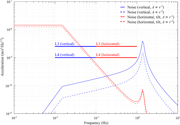
Models of day-time lander mechanical noise recorded by the SEIS instruments given attenuation laws with \(A \propto r^{-1}\) and \(A \propto r^{-2}\). Baseline parameters correspond to those considered in Murdoch et al. (2017). The solar panel resonances are estimated from images of the Phoenix Lander, and the mechanical noise produced by the wind on the lander corresponds to the 70% wind profile. Only vertical forcing is considered, and the conversion of vertical ground forcing into horizontal ground acceleration has been neglected. The horizontal noise plotted in this figure therefore results only from tilt of the seismometer in the Martian gravity field (Sect. 4.2). Also shown are the payload assembly (L3) and SEIS instrument (L4) noise requirements for the VBB (Mimoun et al. 2017; Murdoch et al. 2017)
-
Although teleseismic energy must propagate through the surface layers of regolith to be recorded by the InSight seismometer, the amplitudes of such signals will be less sensitive to these layers relative to local sources (as they will mostly propagate through solid Mars). We therefore expect signal:noise to be somewhat higher than predicted by Murdoch et al. (2017).
-
Our analysis raises the possibility of determining regolith properties (Young’s modulus, Poissons ratio) using noise data returned from the SEIS instruments. The value of Young’s modulus estimated from the tripod resonance in Sect. 5.1 is low compared with literature estimates for similar regolith at 150 kPa confining pressure (2 MPa vs. 20–150 MPa), which suggests that this resonance is largely sensitive to the top few centimeters of regolith. The lower gravity on Mars may also result in a somewhat thicker unconsolidated regolith layer at the InSight landing site, which would reduce the effective Young’s modulus even further.
-
Finally, poor consolidation of sands at the landing site will shift horizontal and vertical signals out of phase. This effect is apparently frequency independent, at least between 5 and 20 Hz. In-depth analysis of particle motions from the InSight data must take this effect into account.

6 Conclusions
In this study, we conducted analogue experiments in Iceland to predict the amplitudes of signals and noise observed by the InSight Mission to Mars, and the effect of mounting the SEIS instruments on a tripod. On the basis of the results of these experiments, we predict that the transfer of noise through the regolith from the InSight lander and WTS will be frequency independent at \(<20\) Hz. Between 3% and 6% of vertical motion of the WTS will be transmitted through the regolith to the SEIS tripod. These values correspond to about 25% and 50% of the values predicted for deformation of a homogeneous elastic half-space. This diminished response is consistent with a small surface Young’s Modulus which exhibits a power-law depth dependence (Sect. 4.4). The amplitude of noise created by motion of the lander will decay as \(A \propto r^{-n}\) where \(1.5< n<2\) within a radius enclosing the potential positions of the SEIS tripod. Given the noise models published for Mars (Mimoun et al. 2017; Murdoch et al. 2017), wind noise should be well-within mission requirements.
Mounting the seismometers on a tripod will not affect the vertical amplitude of recorded signals relative to shallow burial up to a frequency of \(\sim 20\) Hz. Horizontal amplitudes will be affected by mounting the seismometer 10 cm above the surface; whether the amplitudes are increased or decreased depends on the frequency of the displacement. In addition, the vertical particle motions of the tripod-mounted seismometers exhibited a frequency-independent phase lag of \(10\text{--}20 ^{\circ }\) relative to the horizontal motions (Fig. 12). This effect was not observed in motions recorded by the buried seismometer, and is more noticeable on poorly consolidated, sandy ground.
Somewhere between 30 and 80 Hz there will likely be a damped resonance peak between the seismometer and regolith, leading to increased vertical accelerations for a given displacement. The location of this peak should be resolvable using ambient noise, and may provide a good estimate of regolith properties near the surface of Mars. In our analogue experiments, estimated values for Young’s modulus (\(\sim 2\) MPa) are at the very low end of values reported in the literature, suggesting that such values reflect the elastic properties very close to the surface. We point out that signals at frequencies above this resonance (\(>100\) Hz) will be damped as a result of the inertia of the SEIS tripod. This may be beneficial in terms of reducing the chances of clipping due to hammering of the heat flow probe (HP3), which is also a part of the InSight scientific payload.
References
M.S. Alnæs, J. Blechta, J. Hake, A. Johansson, B. Kehlet, A. Logg, C. Richardson, J. Ring, M.E. Rognes, G.N. Wells, The fenics project version 1.5. Arch. Numer. Softw. 3(100) (2015). https://doi.org/10.11588/ans.2015.100.20553
D.L. Anderson, F.K. Duennebier, G.V. Latham, M.F. Toksöz, R.L. Kovach, T.C.D. Knight, A.R. Lazarewicz, W.F. Miller, Y. Nakamura, G. Sutton, The Viking seismic experiment. Science 194(4271), 1318–1321 (1976). https://doi.org/10.1126/science.194.4271.1318
O. Arnalds, F. Gisladottir, H. Sigurjonsson, Sandy deserts of Iceland: an overview. J. Arid Environ. 47(3), 359–371 (2001) https://doi.org/10.1006/jare.2000.0680
W.B. Banerdt, S. Smrekar, L. Alkalai, T. Hoffman, R. Warwick, K. Hurst, W. Folkner, P. Lognonné, T. Spohn, S. Asmar, D. Banfield, L. Boschi, U. Christensen, V. Dehant, D. Giardini, W. Goetz, M. Golombek, M. Grott, T. Hudson, C. Johnson, G. Kargl, N. Kobayashi, J. Maki, D. Mimoun, A. Mocquet, P. Morgan, M. Panning, W.T. Pike, J. Tromp, T. van Zoest, R. Weber, M. Wieczorek (Insight Team), InSight: an integrated exploration of the interior of Mars, in Lunar and Planetary Science Conference, Lunar and Planetary Inst. Technical Report, vol. 43 (2012), p. 2838
M. Beyreuther, R. Barsch, L. Krischer, T. Megies, Y. Behr, J. Wassermann, ObsPy: a python toolbox for seismology. Seismol. Res. Lett. 81(3), 530–533 (2010). https://doi.org/10.1785/gssrl.81.3.530
J.E. Bowles, Foundation Analysis and Design (1996)
N.A. Cabrol, K. Herkenhoff, A.H. Knoll, J. Farmer, R. Arvidson, E. Grin, R. Li, L. Fenton, B. Cohen, J.F. Bell, R. Aileen Yingst, Sands at Gusev Crater, Mars. J. Geophys. Res., Planets 119, 941–967 (2014). https://doi.org/10.1002/2013JE004535
R.T. Clancy, B.J. Sandor, M.J. Wolff, P.R. Christensen, M.D. Smith, J.C. Pearl, B.J. Conrath, R.J. Wilson, An intercomparison of ground-based millimeter, MGS TES, and Viking atmospheric temperature measurements: seasonal and interannual variability of temperatures and dust loading in the global Mars atmosphere. J. Geophys. Res. 105, 9553–9572 (2000). https://doi.org/10.1029/1999JE001089
J.F. Clinton, D. Giardini, P. Lognonné, B. Banerdt, M. van Driel, M. Drilleau, N. Murdoch, M. Panning, R. Garcia, D. Mimoun, M. Golombek, J. Tromp, R. Weber, M. Böse, S. Ceylan, I. Daubar, B. Kenda, A. Khan, L. Perrin, A. Spiga, Preparing for InSight: an invitation to participate in a blind test for Martian seismicity. Seismol. Res. Lett. 88(5), 1290 (2017). https://doi.org/10.1785/0220170094
P.A. Dandonneau, P. Lognonne, W.B. Banerdt, S. Deraucourt, T. Gabsi, J. Gagnepain-Beyneix, T. Nebut, O. Robert, S. Tillier, K. Hurst, D. Mimoun, U. Christenssen, M. Bierwirth, R. Roll, T. Pike, S. Calcutt, D. Giardini, D. Mance, P. Zweifel, P. Laudet, L. Kerjean, R. Perez (Seis Team), The SEIS InSight VBB experiment, in Lunar and Planetary Science Conference, Lunar and Planetary Inst. Technical Report, vol. 44 (2013), p. 2006
P.M. Davis, Meteoroid impacts as seismic sources on Mars. Icarus 105, 469 (1993). https://doi.org/10.1006/icar.1993.1142
P. Delage, F. Karakostas, A. Dhemaied, M. Belmokhtar, P. Lognonné, M. Golombek, E. De Laure, K. Hurst, J.C. Dupla, S. Kedar, Y.J. Cui, B. Banerdt, An investigation of the mechanical properties of some Martian regolith simulants with respect to the surface properties at the InSight mission landing site. Space Sci. Rev. 211, 191–213 (2017). https://doi.org/10.1007/s11214-017-0339-7
A. Delahunty, W. Pike, Metal-armouring for shock protection of MEMS. Sens. Actuators A, Phys. 215, 36–43 (2014). https://doi.org/10.1016/j.sna.2013.11.008
E.A. Flinn, Scientific results of the Viking Project. J. Geophys. Res. 82 (1977)
A. Giannakopoulos, S. Suresh, Indentation of solids with gradients in elastic properties: Part II. Axisymmetric indentors. Int. J. Solids Struct. 34(19), 2393–2428 (1997). https://doi.org/10.1016/S0020-7683(96)00172-2
M.P. Golombek, W.B. Banerdt, K.L. Tanaka, D.M. Tralli, A prediction of Mars seismicity from surface faulting. Science 258, 979–981 (1992). https://doi.org/10.1126/science.258.5084.979
M. Golombek, D. Kipp, N. Warner, I.J. Daubar, R. Fergason, R.L. Kirk, R. Beyer, A. Huertas, S. Piqueux, N.E. Putzig, B.A. Campbell, G.A. Morgan, C. Charalambous, W.T. Pike, K. Gwinner, F. Calef, D. Kass, M. Mischna, J. Ashley, C. Bloom, N. Wigton, T. Hare, C. Schwartz, H. Gengl, L. Redmond, M. Trautman, J. Sweeney, C. Grima, I.B. Smith, E. Sklyanskiy, M. Lisano, J. Benardini, S. Smrekar, P. Lognonné, W.B. Banerdt, Selection of the InSight landing site. Space Sci. Rev. 211, 5–95 (2017). https://doi.org/10.1007/s11214-016-0321-9
R. Greeley, N.T. Bridges, R.O. Kuzmin, J.E. Laity, Terrestrial analogs to wind-related features at the Viking and Pathfinder landing sites on Mars. J. Geophys. Res., Planets 107, 5005 (2002). https://doi.org/10.1029/2000JE001481
W.K. Hartmann, T. Thorsteinsson, F. Sigurdsson, Martian hillside gullies and Icelandic analogs. Icarus 162, 259–277 (2003). https://doi.org/10.1016/S0019-1035(02)00065-9
S. Hempel, R. Garcia, M. Wieczorek, N. Murdoch, The core structure of Mars as expected to be seen by InSight’s VBB seismometer, in EGU General Assembly Conference Abstracts, vol. 18 (2016), p. 8666
S. Kedar, J. Andrade, B. Banerdt, P. Delage, M. Golombek, M. Grott, T. Hudson, A. Kiely, M. Knapmeyer, B. Knapmeyer-Endrun, C. Krause, T. Kawamura, P. Lognonne, T. Pike, Y. Ruan, T. Spohn, N. Teanby, J. Tromp, J. Wookey, Analysis of regolith properties using seismic signals generated by InSight’s HP3 penetrator. Space Sci. Rev. 211, 315–337 (2017). https://doi.org/10.1007/s11214-017-0391-3
A. Khan, M. van Driel, M. Böse, D. Giardini, S. Ceylan, J. Yan, J. Clinton, F. Euchner, P. Lognonné, N. Murdoch, D. Mimoun, M. Panning, M. Knapmeyer, W.B. Banerdt, Single-station and single-event marsquake location and inversion for structure using synthetic Martian waveforms. Phys. Earth Planet. Inter. 258, 28–42 (2016). https://doi.org/10.1016/j.pepi.2016.05.017
M. Knapmeyer, J. Oberst, E. Hauber, M. Wählisch, C. Deuchler, R. Wagner, Working models for spatial distribution and level of Mars’ seismicity. J. Geophys. Res., Planets 111(E10), E11,006 (2006). https://doi.org/10.1029/2006JE002708
A.R. Lazarewicz, D.L. Anderson, K. Anderson, A.M. Daonty, F.K. Duennebier, N.R. Gains, T.C.D. Knight, R.L. Kovach, G.V. Latham, W.F. Miller, The Viking seismometry. Tech. rep. (1981)
A. Logg, K.A. Mardal, G.N. Wells, Automated Solution of Differential Equations by the Finite Element Method: The FEniCS Book, vol. 84 (Springer, Berlin, 2012). https://doi.org/10.1007/978-3-642-23099-8
P. Lognonne, W. Banerdt, T. Pike, D. Giardini, U. Christensen, D. Banfield, D. Mimoun, P. Laudet, S. de Raucourt, M. Bierwirth, P. Zweifel, S. Calcutt, K. Hurst, C. Bruce, SEIS/INSIGHT and Mars seismology: development status and focus on the impact detection, in EGU General Assembly Conference Abstracts, vol. 16 (2014), p. 12183
R.D. Lorenz, Y. Nakamura, J.R. Murphy, Viking-2 seismometer measurements on Mars: PDS data archive and meteorological applications. Earth Space Sci. 4(11), 681–688 (2017). https://doi.org/10.1002/2017EA000306
H.B. Mattsson, Á Höskuldsson, Contemporaneous phreatomagmatic and effusive activity along the Hverfjall eruptive fissure, North Iceland: eruption chronology and resulting deposits. J. Volcanol. Geotherm. Res. 201, 241–252 (2011). https://doi.org/10.1016/j.jvolgeores.2010.05.015
D. Mimoun, P. Lognonné, W.B. Banerdt, K. Hurst, S. Deraucourt, J. Gagnepain-Beyneix, T. Pike, S. Calcutt, M. Bierwirth, R. Roll, P. Zweifel, D. Mance, O. Robert, T. Nébut, S. Tillier, P. Laudet, L. Kerjean, R. Perez, D. Giardini, U. Christenssen, R. Garcia, The InSight SEIS experiment, in Lunar and Planetary Science Conference, Lunar and Planetary Inst. Technical Report, vol. 43 (2012), p. 1493
D. Mimoun, N. Murdoch, P. Lognonné, K. Hurst, W.T. Pike, J. Hurley, T. Nébut, W.B. Banerdt, The noise model of the seis seismometer of the insight mission to Mars. Space Sci. Rev. 211(1), 383–428 (2017). https://doi.org/10.1007/s11214-017-0409-x
N. Murdoch, D. Mimoun, R.F. Garcia, W. Rapin, T. Kawamura, P. Lognonné, D. Banfield, W.B. Banerdt, Evaluating the wind-induced mechanical noise on the InSight seismometers. Space Sci. Rev. 211, 429–455 (2017). https://doi.org/10.1007/s11214-016-0311-y. 1612.04308
M.P. Panning, É Beucler, M. Drilleau, A. Mocquet, P. Lognonné, W.B. Banerdt, Verifying single-station seismic approaches using Earth-based data: preparation for data return from the InSight mission to Mars. Icarus 248, 230–242 (2015). https://doi.org/10.1016/j.icarus.2014.10.035
M.P. Panning, P. Lognonné, W. Bruce Banerdt, R. Garcia, M. Golombek, S. Kedar, B. Knapmeyer-Endrun, A. Mocquet, N.A. Teanby, J. Tromp, R. Weber, E. Beucler, J.F. Blanchette-Guertin, E. Bozdağ, M. Drilleau, T. Gudkova, S. Hempel, A. Khan, V. Lekić, N. Murdoch, A.C. Plesa, A. Rivoldini, N. Schmerr, Y. Ruan, O. Verhoeven, C. Gao, U. Christensen, J. Clinton, V. Dehant, D. Giardini, D. Mimoun, W. Thomas Pike, S. Smrekar, M. Wieczorek, M. Knapmeyer, J. Wookey, Planned products of the Mars structure service for the InSight mission to Mars. Space Sci. Rev. 211, 611–650 (2017). https://doi.org/10.1007/s11214-016-0317-5
R.J. Phillips, R.E. Grimm, Martian seismicity, in Lunar and Planetary Science Conference, vol. 22 (1991)
W.T. Pike, I.M. Standley, W.B. Banerdt, A high-sensitivity broad-band seismic sensor for shallow seismic sounding of the lunar regolith, in 36th Annual Lunar and Planetary Science Conference, Lunar and Planetary Inst. Technical Report, vol. 36, ed. by S. Mackwell, E. Stansbery (2005)
G.P. Roberts, B. Matthews, C. Bristow, L. Guerrieri, J. Vetterlein, Possible evidence of paleomarsquakes from fallen boulder populations, Cerberus Fossae, Mars. J. Geophys. Res., Planets 117(E2), e02009 (2012). https://doi.org/10.1029/2011JE003816
J. Santamarina, K.A. Klein, M.A. Fam, Soils and Waves: Particulate Materials Behavior, Characterization and Process Monitoring (Wiley, New York, 2001)
J.T. Schofield, J.R. Barnes, D. Crisp, R.M. Haberle, S. Larsen, J.A. Magalhaes, J.R. Murphy, A. Seiff, G. Wilson, The Mars pathfinder atmospheric structure investigation/meteorology. Science 278, 1752 (1997). https://doi.org/10.1126/science.278.5344.1752
I.N. Sneddon, Boussinesq’s problem for a flat-ended cylinder. Proc. Camb. Philos. Soc. 42, 29 (1946). https://doi.org/10.1017/S0305004100022702
J. Stevanović, N.A. Teanby, J. Wookey, N. Selby, I.J. Daubar, J. Vaubaillon, R. Garcia, Bolide airbursts as a seismic source for the 2018 Mars InSight mission. Space Sci. Rev. 211, 525–545 (2017). https://doi.org/10.1007/s11214-016-0327-3
J. Taylor, N.A. Teanby, J. Wookey, Estimates of seismic activity in the Cerberus Fossae region of Mars. J. Geophys. Res., Planets 118, 2570–2581 (2013). https://doi.org/10.1002/2013JE004469
N.A. Teanby, Predicted detection rates of regional-scale meteorite impacts on Mars with the InSight short-period seismometer. Icarus 256, 49–62 (2015). https://doi.org/10.1016/j.icarus.2015.04.012
N.A. Teanby, J. Wookey, Seismic detection of meteorite impacts on Mars. Phys. Earth Planet. Inter. 186, 70–80 (2011). https://doi.org/10.1016/j.pepi.2011.03.004
N.A. Teanby, J. Stevanović, J. Wookey, N. Murdoch, J. Hurley, R. Myhill, N.E. Bowles, S.B. Calcutt, W.T. Pike, Seismic coupling of short-period wind noise through Mars’ regolith for NASA’s InSight lander. Space Sci. Rev. 211, 485–500 (2017). https://doi.org/10.1007/s11214-016-0310-z
N.H. Warner, M.P. Golombek, J. Sweeney, R. Fergason, R. Kirk, C. Schwartz, Near surface stratigraphy and regolith production in southwestern Elysium Planitia, Mars: implications for Hesperian-Amazonian terrains and the InSight lander mission. Space Sci. Rev. 211, 147–190 (2017). https://doi.org/10.1007/s11214-017-0352-x
P. Wessel, W.H.F. Smith, R. Scharroo, J. Luis, F. Wobbe, Generic mapping tools: improved version released. EOS Trans. 94, 409–410 (2013). https://doi.org/10.1002/2013EO450001
Acknowledgements
This research was funded by UK Space Agency (UKSA) Aurora Grants to R.M. and N.T.. The authors would like to thank Charles Clapham and Donovan Hawley for fabrication work involved with the field experiments, without which this work would have been impossible. R.M. would like to thank Charlotte Gilder for invaluable discussions, and two anonymous reviewers whose careful and insightful comments significantly improved the manuscript. Seismic analysis was conducted using the python toolbox ObsPy (Beyreuther et al. 2010). The map figure was created using the Generic Mapping Tools (Wessel et al. 2013). Other figures were created with the python matplotlib module.
Author information
Authors and Affiliations
Corresponding author
Additional information
The InSight Mission to Mars II
Edited by William B. Banerdt and Christopher T. Russell
Electronic Supplementary Material
Below is the link to the electronic supplementary material.
Rights and permissions
Open Access This article is distributed under the terms of the Creative Commons Attribution 4.0 International License (http://creativecommons.org/licenses/by/4.0/), which permits unrestricted use, distribution, and reproduction in any medium, provided you give appropriate credit to the original author(s) and the source, provide a link to the Creative Commons license, and indicate if changes were made.
About this article

Cite this article
Myhill, R., Teanby, N.A., Wookey, J. et al. Near-Field Seismic Propagation and Coupling Through Mars’ Regolith: Implications for the InSight Mission. Space Sci Rev 214, 85 (2018). https://doi.org/10.1007/s11214-018-0514-5
Received:
Accepted:
Published:
DOI: https://doi.org/10.1007/s11214-018-0514-5