Ncorr: Open-Source 2D Digital Image Correlation Matlab Software

Abstract

Digital Image Correlation (DIC) is an important and widely used non-contact technique for measuring material deformation. Considerable progress has been made in recent decades in both developing new experimental DIC techniques and in enhancing the performance of the relevant computational algorithms. Despite this progress, there is a distinct lack of a freely available, high-quality, flexible DIC software. This paper documents a new DIC software package Ncorr that is meant to fill that crucial gap. Ncorr is an open-source subset-based 2D DIC package that amalgamates modern DIC algorithms proposed in the literature with additional enhancements. Several applications of Ncorr that both validate it and showcase its capabilities are discussed.

Appendices

Appendix A1. The Gradient and Hessian Quantities

In order to simplify the calculations, the following assumptions are used

$$ \frac{d}{d\boldsymbol{p}}\left({f}_m\right)\approx 0 $$

(19)

$$ \frac{d}{d\boldsymbol{p}}\left(\sqrt{{{\displaystyle \sum \left[f\left({\boldsymbol{\xi}}_{{\mathrm{ref}}_{\mathrm{c}}}+w\left(\varDelta {\boldsymbol{\xi}}_{ref};\mathbf{0}\right)\right)-{f}_m\right]}}^2}\right)\approx 0 $$

(20)

The gradient for the IC-GN method based on equation (10) is

$$ \begin{array}{l}\nabla {C}_{LS}\left(\mathbf{0}\right)=\frac{d{C}_{LS}\left(\mathbf{0}\right)}{d\boldsymbol{p}}\hfill \\ {}\approx \frac{2}{\sqrt{{{\displaystyle \sum \left[f\left({\boldsymbol{\xi}}_{{\mathrm{ref}}_{\mathrm{c}}}+w\left(\varDelta {\boldsymbol{\xi}}_{\boldsymbol{ref}};\mathbf{0}\right)\right)-{f}_m\right]}}^2}}{\displaystyle \sum \left[\left[\frac{f\left({\boldsymbol{\xi}}_{{\mathrm{ref}}_{\mathrm{c}}}+w\left(\varDelta {\boldsymbol{\xi}}_{\boldsymbol{ref}};\mathbf{0}\right)\right)-{f}_m}{\sqrt{{\displaystyle \sum {\left[f\left({\boldsymbol{\xi}}_{{\mathrm{ref}}_{\mathrm{c}}}+w\left(\varDelta {\boldsymbol{\xi}}_{\boldsymbol{ref}};\mathbf{0}\right)\right)-{f}_m\right]}^2}}}\right.\right.}\hfill \\ {}\left.\left.-\frac{g\left({\boldsymbol{\xi}}_{{\mathrm{ref}}_{\mathrm{c}}}+w\left(\varDelta {\boldsymbol{\xi}}_{\boldsymbol{ref}};{\boldsymbol{p}}_{\boldsymbol{old}}\right)\right)-{g}_m}{\sqrt{{{\displaystyle \sum \left[g\left({\boldsymbol{\xi}}_{{\mathrm{ref}}_{\mathrm{c}}}+w\left(\varDelta {\boldsymbol{\xi}}_{\boldsymbol{ref}};{\boldsymbol{p}}_{\boldsymbol{old}}\right)\right)-{g}_m\right]}}^2}}\right]\left[\frac{d}{d\boldsymbol{p}}f\left({\boldsymbol{\xi}}_{{\mathrm{ref}}_{\mathrm{c}}}+w\left(\varDelta {\boldsymbol{\xi}}_{\boldsymbol{ref}};\mathbf{0}\right)\right)\right]\right]\hfill \end{array} $$

(21)

The hessian is

$$ \begin{array}{l}\nabla \nabla {C}_{LS}\left(\mathbf{0}\right)=\frac{d^2{C}_{LS}\left(\mathbf{0}\right)}{d{\boldsymbol{p}}^2}\hfill \\ {}\approx \frac{2}{\sqrt{{\displaystyle \sum {\left[f\left({\boldsymbol{\xi}}_{{\mathrm{ref}}_{\mathrm{c}}}+w\left(\varDelta {\boldsymbol{\xi}}_{\boldsymbol{ref}};\mathbf{0}\right)\right)-{f}_m\right]}^2}}}\left\{{\displaystyle \sum \left[\frac{\frac{d}{d\boldsymbol{p}}f\left({\boldsymbol{\xi}}_{{\mathrm{ref}}_{\mathrm{c}}}+w\left(\varDelta {\boldsymbol{\xi}}_{\boldsymbol{ref}};\mathbf{0}\right)\right)}{\sqrt{{\displaystyle \sum {\left[f\left({\boldsymbol{\xi}}_{{\mathrm{ref}}_{\mathrm{c}}}+w\left(\varDelta {\boldsymbol{\xi}}_{\boldsymbol{ref}};\mathbf{0}\right)\right)-{f}_m\right]}^2}}}\right]}\left[\frac{d}{d\boldsymbol{p}}f\left({\boldsymbol{\xi}}_{{\mathrm{ref}}_{\mathrm{c}}}+\right.\right.\right.\hfill \\ {}{\left.\left.w\left(\varDelta {\boldsymbol{\xi}}_{\boldsymbol{ref}};\mathbf{0}\right)\right)\right]}^T+{\displaystyle \sum \left[\frac{f\left({\boldsymbol{\xi}}_{{\mathrm{ref}}_{\mathrm{c}}}+w\left(\varDelta {\boldsymbol{\xi}}_{\boldsymbol{ref}};0\right)\right)-{f}_m}{\sqrt{{\displaystyle \sum \left[f\left({\boldsymbol{\xi}}_{{\mathrm{ref}}_{\mathrm{c}}}+w\left(\varDelta {\boldsymbol{\xi}}_{\boldsymbol{ref}};\mathbf{0}\right)\right)-{f}_m\right]}}}-\frac{g\left({\boldsymbol{\xi}}_{{\mathrm{ref}}_{\mathrm{c}}}+w\left(\varDelta {\boldsymbol{\xi}}_{\boldsymbol{ref}};{\boldsymbol{p}}_{\boldsymbol{old}}\right)\right)-{g}_m}{\sqrt{{{\displaystyle \sum \left[g\left({\boldsymbol{\xi}}_{{\mathrm{ref}}_{\mathrm{c}}}+w\left(\varDelta {\boldsymbol{\xi}}_{\boldsymbol{ref}};{\boldsymbol{p}}_{\boldsymbol{old}}\right)\right)-{g}_m\right]}}^2}}\right]}\hfill \\ {}\left.\left[\frac{d^2}{d\boldsymbol{p}}f\left({\boldsymbol{\xi}}_{{\mathrm{ref}}_{\mathrm{c}}}+w\left(\varDelta {\boldsymbol{\xi}}_{\boldsymbol{ref}};\mathbf{0}\right)\right)\right]\right\}\hfill \end{array} $$

(22)

Using the Gauss-Newton assumption

$$ {\displaystyle \sum \left[\frac{f\left({\boldsymbol{\xi}}_{{\mathrm{ref}}_{\mathrm{c}}}+w\left(\varDelta {\boldsymbol{\xi}}_{\boldsymbol{ref}};\mathbf{0}\right)\right)-{f}_m}{{\displaystyle \sum {\left[f\left({\boldsymbol{\xi}}_{{\mathrm{ref}}_{\mathrm{c}}}+w\left(\varDelta {\boldsymbol{\xi}}_{\boldsymbol{ref}};\mathbf{0}\right)\right)-{f}_m\right]}^2}}-\frac{g\left({\boldsymbol{\xi}}_{{\mathrm{ref}}_{\mathrm{c}}}+w\left(\varDelta {\boldsymbol{\xi}}_{\boldsymbol{ref}};{\boldsymbol{p}}_{\boldsymbol{old}}\right)\right)-{g}_m}{\sqrt{{\displaystyle \sum {\left[g\left({\boldsymbol{\xi}}_{{\mathrm{ref}}_{\mathrm{c}}}+w\left(\varDelta {\boldsymbol{\xi}}_{\boldsymbol{ref}};{\boldsymbol{p}}_{\boldsymbol{old}}\right)\right)-{g}_m\right]}^2}}}\right]\left[\frac{d^2}{d{\boldsymbol{p}}^2}f\left({\boldsymbol{\xi}}_{{\mathrm{ref}}_{\mathrm{c}}}+w\left(\varDelta {\boldsymbol{\xi}}_{\boldsymbol{ref}};\mathbf{0}\right)\right)\right]\approx 0} $$

(23)

yields the hessian in the final form

$$ \begin{array}{c}\hfill \nabla \nabla {C}_{LS}\left(\mathbf{0}\right)\approx \frac{d{C}_{LS}\left(\mathbf{0}\right)}{d{\boldsymbol{p}}^2}\hfill \\ {}\hfill \approx \frac{2}{{\displaystyle \sum {\left[f\left({\boldsymbol{\xi}}_{{\mathrm{ref}}_{\mathrm{c}}}+w\left(\varDelta {\boldsymbol{\xi}}_{\boldsymbol{ref}};\mathbf{0}\right)\right)-{f}_m\right]}^2}}{\displaystyle \sum \left[\frac{d}{d\boldsymbol{p}}f\left({\boldsymbol{\xi}}_{{\mathrm{ref}}_{\mathrm{c}}}\right.\right.}\hfill \\ {}\hfill \left.\left.+\kern0.5em w\left(\varDelta {\boldsymbol{\xi}}_{\boldsymbol{ref}};\mathbf{0}\right)\right)\right]{\left[\frac{d}{d\boldsymbol{p}}f\left({\boldsymbol{\xi}}_{{\mathrm{ref}}_{\mathrm{c}}}+w\left(\varDelta {\boldsymbol{\xi}}_{\boldsymbol{ref}};\mathbf{0}\right)\right)\right]}^T\hfill \end{array} $$

(24)

Appendix A2. Biquintic B-Spline Interpolation

The quantities $\frac{d}{d\boldsymbol{p}}f\left({\boldsymbol{\xi}}_{{\mathrm{ref}}_{\mathrm{c}}}+w\left(\varDelta {\boldsymbol{\xi}}_{\boldsymbol{ref}};\mathbf{0}\right)\right)$ and $g\left({\boldsymbol{\xi}}_{{\mathrm{ref}}_{\mathrm{c}}}+w\left(\varDelta {\boldsymbol{\xi}}_{\boldsymbol{ref}};{\boldsymbol{p}}_{\boldsymbol{old}}\right)\right)$ require some form of estimation through interpolation. Using the chain rule on $\frac{d}{d\boldsymbol{p}}f\left({\boldsymbol{\xi}}_{{\mathrm{ref}}_{\mathrm{c}}}+w\left(\varDelta {\boldsymbol{\xi}}_{\boldsymbol{ref}};\mathbf{0}\right)\right)$ and equation (4), we obtain:

$$ \frac{d}{d\boldsymbol{p}}f\left({\tilde{x}}_{re{f}_i},{\tilde{y}}_{re{f}_j}\right)=\frac{\partial }{\partial {\tilde{x}}_{re{f}_i}}f\left({\tilde{x}}_{re{f}_i},{\tilde{y}}_{re{f}_j}\right)\ast \frac{d{\tilde{x}}_{re{f}_i}}{d\boldsymbol{p}}+\frac{\partial }{\partial {\tilde{y}}_{re{f}_j}}f\left({\tilde{x}}_{re{f}_i},{\tilde{y}}_{re{f}_j}\right)\ast \frac{d{\tilde{y}}_{re{f}_j}}{d\boldsymbol{p}} $$

(25)

The only two quantities we need to specifically compute for equation (25) are $\frac{\partial }{\partial {\tilde{x}}_{re{f}_i}}f\left({\tilde{x}}_{re{f}_i},{\tilde{y}}_{re{f}_j}\right)$ and $\frac{\partial }{\partial {\tilde{y}}_{re{f}_j}}f\left({\tilde{x}}_{re{f}_i},{\tilde{y}}_{re{f}_j}\right)$. These can be computed in various ways (sobel filter, finite difference, etc.), but in Ncorr, biquintic B-spline interpolation is used.

The quantity $g\left({\boldsymbol{\xi}}_{{\mathrm{ref}}_{\mathrm{c}}}+w\left(\varDelta {\boldsymbol{\xi}}_{\boldsymbol{ref}};{\boldsymbol{p}}_{\boldsymbol{old}}\right)\right)$ also requires interpolation. Once $\frac{\partial }{\partial {\tilde{x}}_{re{f}_i}}f\left({\tilde{x}}_{re{f}_i},{\tilde{y}}_{re{f}_j}\right)$ and $\frac{\partial }{\partial {\tilde{y}}_{re{f}_j}}f\left({\tilde{x}}_{re{f}_i},{\tilde{y}}_{re{f}_j}\right)$ are precomputed for the entire reference image, and $g\left({\boldsymbol{\xi}}_{{\mathrm{ref}}_{\mathrm{c}}}+w\left(\varDelta {\boldsymbol{\xi}}_{\boldsymbol{ref}};{\boldsymbol{p}}_{\boldsymbol{old}}\right)\right)$ is computable, equation (19) and equation (22) can be computed and iterated with equation (10) to find a closer approximation to p ^∗_rc .

The main idea behind B-spline interpolation is to approximate the image grayscale surface with a linear combination of B-spline basis “splines.” These splines are scaled via the B-spline coefficients and then the linear combination of these scaled splines forms an approximation of the surface. Once this approximation is complete, points can be interpolated through 1-D convolutions (since biquintic B-spline interpolation is separable [49]), which reduces to a series of simple dot products. The equation for interpolation for the 1D case is

$$ g(x)={\displaystyle \sum_{k\in Z}c(k){\beta}^n\left(x-k\right)} $$

(26)

where c(k),βⁿ(x − k), and g(x) are the B-spline coefficient value at integer k, the B-spline kernel value at x − k, and the interpolated signal value at x, respectively. Here n is the B-spline kernel order, which is set to 5 (the quintic kernel) and Z is the set of integers. Note that the B-spline coefficients are not equivalent to the data samples (unlike in other forms of interpolation—i.e. bicubic keys [50]), and thus must be solved for directly. The equation for the B-spline kernel is

$$ {\beta}^n(x)=\frac{1}{n!}{\displaystyle \sum_{k=0}^{n+1}\left(\begin{array}{c}\hfill n+1\hfill \\ {}\hfill k\hfill \end{array}\right){\left(-1\right)}^k{\left(x-k+\frac{n+1}{2}\right)}_{+}^n} $$

(27)

When solved for the quintic case, this equation yields:

$$ {\beta}^5(x)=\left\{\begin{array}{ll}\frac{1}{120}{x}^5+\frac{1}{8}{x}^4+\frac{3}{4}{x}^3+\frac{9}{4}{x}^2+\frac{27}{8}x+\frac{81}{40}\hfill & -2\ge x\ge -3\hfill \\ {}-\frac{1}{24}{x}^5-\frac{3}{8}{x}^4-\frac{5}{4}{x}^3-\frac{7}{4}{x}^2-\frac{5}{8}{x}^2+\frac{17}{40}\hfill & -1\ge x\ge -2\hfill \\ {}\frac{1}{12}{x}^5+\frac{1}{4}{x}^4-\frac{1}{2}{x}^2+\frac{11}{20}\hfill & 0\kern0.5em x\ge -1\hfill \\ {}-\frac{1}{12}{x}^5-\frac{3}{8}{x}^4+\frac{5}{4}{x}^3-\frac{7}{4}{x}^2+\frac{5}{8}x+\frac{17}{40}\hfill & 1\kern0.5em x\ge 1\hfill \\ {}\frac{1}{24}{x}^5-\frac{3}{8}{x}^4+\frac{5}{4}{x}^3-\frac{7}{4}{x}^2+\frac{5}{8}x+\frac{17}{40}\hfill & 2\kern0.5em x\ge 1\hfill \\ {}-\frac{1}{120}{x}^5+\frac{1}{8}{x}^4-\frac{3}{4}{x}^3+\frac{9}{4}{x}^2-\frac{27}{8}x+\frac{81}{40}\hfill & 30x\ge 2\hfill \end{array}\right. $$

(28)

The first step of the interpolation process is to determine the B-spline coefficients. They can be found by using deconvolution. Applying Discrete Fourier Transform (DFT) to equation (26) yields:

$$ F\left\{g\right\}=F\left\{c\right\}\ast F\left\{{\beta}^{\mathrm{n}}\right\} $$

(29)

where F{…} is the DFT. The goal is to solve for c, the B-spline coefficients. This can be done by dividing the Fourier coefficients of the B-spline kernel element-wise with the Fourier coefficients of the signal as shown:

$$ F\left\{c\right\}=\frac{F\left\{{\beta}^{\mathrm{n}}\right\}}{F\left\{g\right\}} $$

(30)

Taking the inverse DFT of equation (30) will then yield the B-spline coefficients, although caution should be exercised when using this method due to the circular nature of the DFT. To mitigate wrap-around errors, padding should be used.

After obtaining the B-spline coefficients, the image array can be interpolated point-wise by using equation (26). This is carried out by taking a series of dot products with the columns of the B-spline coefficient array and B-spline kernel, and then taking a single dot product across the resulting row of interpolated B-spine coefficient values (note that the order of this operation doesn’t matter). The first step of the aforementioned process can be thought of as interpolating the 2D B-spline grid to obtain 1D B-spline coefficient values, and then the second step as interpolating the grayscale value from these 1D B-spline coefficient values.

The steps for obtaining the B-spline coefficients are outlined below:

• 1. Make a copy of the grayscale array and pad it (any method can be used; Ncorr uses the border values to expand the data as shown in the top right of Fig. 14(a)). Then, sample the B-spline kernel at −2,−1,0,1, 2, and 3. This will form the quintic B-spline vector

  Fig. 14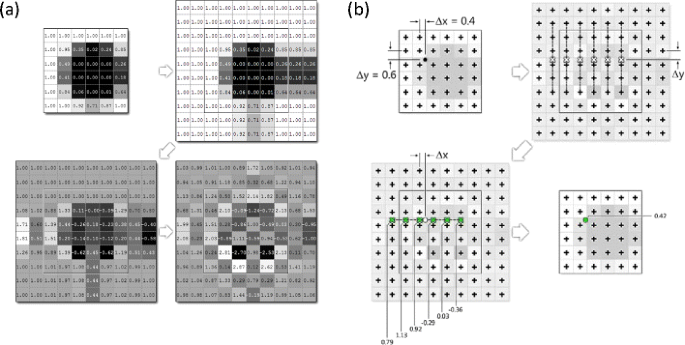

  

  (a) Schematic of the B-spline coefficient calculation. Top-left: original grayscale values array. Top-right: Copy and pad data; padding parameter here is set to 2. Bottom-left: Deconvolution via the DFT for each row and then each column. Bottom-right: The associated B-spline coefficients for the top-left image. (b) Extension of (a) with the same gray scale and B-spline coefficients. Black crosses represent integer pixel locations and the black circle (top-left) is the subpixel point being interpolated

  $$ {\mathrm{b}}_{\mathrm{o}}={\left\{\begin{array}{llllll}1/120\hfill & 13/60\hfill & 11/20\hfill & 13/60\hfill & 1/120\hfill & 0\hfill \end{array}\right\}}^{\mathrm{T}} $$

  (31)

• 2. Pad the kernel with zeros to the same size as the number of columns (the width) of the image grayscale array. Take the FFT of the padded kernel, and then store it in place.

• 3. Take the FFT of an image row, then divide the Fourier coefficients element-wise of the padded B-spline with the Fourier coefficients from the image row. Afterward, take the inverse FFT of the results and store them in place (in the padded grayscale array). This is done for all the image rows as shown on the bottom right of Fig. 14(a).

• 4. Repeat steps 2–3, except column-wise, with the array obtained at the end of step 3. The result will be the B-spline coefficients of original image array as shown on the bottom right of Fig. 14(a).

Now that the B-spline coefficients have been obtained, we can interpolate values at sub pixel locations. The steps are outlined below:

• 1. Pick a subpixel point, $\left({\tilde{x}}_{cur},{\tilde{y}}_{cur}\right)$, within the image array to interpolate.

• 2. Calculate Δx and Δy, where:

  $$ \begin{array}{c}\hfill \varDelta x={\tilde{x}}_{cur}-{x}_f\hfill \\ {}\hfill \varDelta y={\tilde{y}}_{cur}-{y}_f\hfill \end{array} $$

  (32)

  where x_f = floor(${\tilde{x}}_{cur}$) and y_f = floor(ỹ _cur ).

• 3. Perform the operation in equation (32) to obtain the interpolated grayscale value.

  $$ g\left({\tilde{x}}_{cur},{\tilde{y}}_{cur}\right)=\left[\begin{array}{llllll}1\hfill & \varDelta y\hfill & \varDelta {y}^2\hfill & \varDelta {y}^3\hfill & \varDelta {y}^4\hfill & \varDelta {y}^5\hfill \end{array}\right]\left[QK\right]\left[c\right]{}_{\left({x}_f-2:{x}_f+3,{y}_f-2:{y}_f+3\right)}{\left[QK\right]}^T\left[\begin{array}{c}\hfill 1\hfill \\ {}\hfill \varDelta x\hfill \\ {}\hfill \varDelta {x}^2\hfill \\ {}\hfill \varDelta {x}^3\hfill \\ {}\hfill \varDelta {x}^4\hfill \\ {}\hfill \varDelta {x}^5\hfill \end{array}\right] $$

  (33)

  where [QK] is the array defined:

  $$ \left[QK\right]=\left[\begin{array}{cccccc}\hfill \frac{1}{120}\hfill & \hfill \frac{13}{60}\hfill & \hfill \frac{11}{20}\hfill & \hfill \frac{13}{60}\hfill & \hfill \frac{1}{120}\hfill & \hfill 0\hfill \\ {}\hfill -\frac{1}{24}\hfill & \hfill -\frac{5}{12}\hfill & \hfill 0\hfill & \hfill \frac{5}{12}\hfill & \hfill \frac{1}{24}\hfill & \hfill 0\hfill \\ {}\hfill \frac{1}{12}\hfill & \hfill \frac{1}{6}\hfill & \hfill -\frac{1}{2}\hfill & \hfill \frac{1}{6}\hfill & \hfill \frac{1}{12}\hfill & \hfill 0\hfill \\ {}\hfill -\frac{1}{12}\hfill & \hfill \frac{1}{6}\hfill & \hfill 0\hfill & \hfill -\frac{1}{6}\hfill & \hfill \frac{1}{12}\hfill & \hfill 0\hfill \\ {}\hfill \frac{1}{24}\hfill & \hfill -\frac{1}{6}\hfill & \hfill \frac{1}{4}\hfill & \hfill -\frac{1}{6}\hfill & \hfill \frac{1}{24}\hfill & \hfill 0\hfill \\ {}\hfill -\frac{1}{120}\hfill & \hfill \frac{1}{24}\hfill & \hfill -\frac{1}{12}\hfill & \hfill \frac{1}{12}\hfill & \hfill -\frac{1}{24}\hfill & \hfill \frac{1}{120}\hfill \end{array}\right] $$

  (34)

  and${\left[c\right]}_{\left({x}_f-2:{x}_f+3,{y}_f-2:{y}_f+3\right)}$ are the B-spline coefficients as shown:

  $$ {\left[c\right]}_{\left({x}_f-2:{x}_f+3,{y}_f-2:{y}_f+3\right)}=\left[\begin{array}{cccccc}\hfill {c}_{\left({x}_f-2,{y}_f-2\right)}\hfill & \hfill {c}_{\left({x}_f-1,{y}_f-2\right)}\hfill & \hfill {c}_{\left({x}_f,{y}_f-2\right)}\hfill & \hfill {c}_{\left({x}_f+1,{y}_f-22\right)}\hfill & \hfill {c}_{\left({x}_f+2,{y}_f-2\right)}\hfill & \hfill {c}_{\left({x}_f+3,{y}_f-2\right)}\hfill \\ {}\hfill {c}_{\left({x}_f-2,{y}_f-1\right)}\hfill & \hfill {c}_{\left({x}_f-1,{y}_f-1\right)}\hfill & \hfill {c}_{\left({x}_f+1,{y}_f-1\right)}\hfill & \hfill {c}_{\left({x}_f+1,{y}_f-1\right)}\hfill & \hfill {c}_{\left({x}_f+2,{y}_f-1\right)}\hfill & \hfill {c}_{\left({x}_f+3,{y}_f-1\right)}\hfill \\ {}\hfill {c}_{\left({x}_f-2,{y}_f\right)}\hfill & \hfill {c}_{\left({x}_f-1,{y}_f\right)}\hfill & \hfill {c}_{\left({x}_f,{y}_f\right)}\hfill & \hfill {c}_{\left({x}_f+1,{y}_f\right)}\hfill & \hfill {c}_{\left({x}_f+2,{y}_f\right)}\hfill & \hfill {c}_{\left({x}_f+3,{y}_f\right)}\hfill \\ {}\hfill {c}_{\left({x}_f-2,{y}_f+1\right)}\hfill & \hfill {c}_{\left({x}_f-1,{y}_f+1\right)}\hfill & \hfill {c}_{\left({x}_f+1,{y}_f+1\right)}\hfill & \hfill {c}_{\left({x}_f+1,{y}_f+1\right)}\hfill & \hfill {c}_{\left({x}_f+2,{y}_f+1\right)}\hfill & \hfill {c}_{\left({x}_f+3,{y}_f+1\right)}\hfill \\ {}\hfill {c}_{\left({x}_f-2,{y}_f+2\right)}\hfill & \hfill {c}_{\left({x}_f-1,{y}_f+2\right)}\hfill & \hfill {c}_{\left({x}_f,{y}_f+2\right)}\hfill & \hfill {c}_{\left({x}_f+1,{y}_f+2\right)}\hfill & \hfill {c}_{\left({x}_f+2,{y}_f+2\right)}\hfill & \hfill {c}_{\left({x}_f+3,{y}_f+2\right)}\hfill \\ {}\hfill {c}_{\left({x}_f-2,{y}_f+3\right)}\hfill & \hfill {c}_{\left({x}_f-1,{y}_f+3\right)}\hfill & \hfill {c}_{\left({x}_f,{y}_f+3\right)}\hfill & \hfill {c}_{\left({x}_f+1,{y}_f+3\right)}\hfill & \hfill {c}_{\left({x}_f+2,{y}_f+3\right)}\hfill & \hfill {c}_{\left({x}_f+3,{y}_f+3\right)}\hfill \end{array}\right] $$

  (35)

The position of the required B-spline coefficients within the B-spline array ultimately depends on the amount of padding used. Figure 14(b) gives an example of the location of the coefficients within the B-spline array for a given x_f and y_f and a padding of 2.

The left portion containing the ∆y vector and the [QK] matrix is the matrix form of resampling the quintic B-spline kernel with a shift of ∆y. Right multiplying this quantity by ${\left[c\right]}_{\left({x}_f=2:{x}_f+3,{y}_f-2:{y}_f+3\right)}$ yields the interpolated B-spline coefficients which form a row of values, as shown in the top right of Fig. 14(b). When this quantity is right multiplied by [QK] and the ∆x vector, it interpolates the gray-scale value we need from the interpolated row of B-spline coefficients as shown on the bottom left of Fig. 14(b).

Lastly, examining the portion central portion containing:

$$ \left[QK\right]{\left[c\right]}_{\left({x}_f-2:{x}_f+3,{y}_f-2:{y}_f+3\right)}{\left[QK\right]}^T $$

(36)

this term can be precomputed to increase the speed of the program [37]. This precomputation for biquintic B-spline interpolation requires a very large amount of storage (36 times the size of the padded B-spline coefficient array). But, the space required may be worth the trade off for the speed improvement. The largest computational bottleneck in the DIC analysis is the interpolation step when calculating the components of the hessian, so the reduction in computational time is worth the expensive memory requirement.

At this point, the $g\left({\tilde{x}}_{cu{r}_i},{\tilde{y}}_{cu{r}_j}\right)$ quantity is calculable. The last quantities to address are $\frac{\partial }{\partial {\tilde{x}}_{ref}}f\left({\tilde{x}}_{re{f}_i},{\tilde{y}}_{re{f}_j}\right)$ and $\frac{\partial }{\partial {\tilde{y}}_{ref}}f\left({\tilde{x}}_{re{f}_i},{\tilde{y}}_{re{f}_j}\right)$. These quantities can be computed by taking the partial derivatives of an equation of the same form as equation (33) and setting Δx and Δy to zero (because these are integer pixel locations) to obtain

$$ \frac{\partial }{\partial {\tilde{x}}_{ref}}f\left({\tilde{x}}_{re{f}_i},{\tilde{y}}_{re{f}_j}\right)=\left[\begin{array}{cccccc}\hfill 1\hfill & \hfill 0\hfill & \hfill 0\hfill & \hfill 0\hfill & \hfill 0\hfill & \hfill 0\hfill \end{array}\right]\ast \left[QK\right]\ast {\left[c\right]}_{\left({x}_f-2:{x}_f+3,{y}_f-2:{y}_f+3\right)}\ast {\left[QK\right]}^T\ast \left[\begin{array}{c}\hfill 0\hfill \\ {}\hfill 1\hfill \\ {}\hfill 0\hfill \\ {}\hfill 0\hfill \\ {}\hfill 0\hfill \\ {}\hfill 0\hfill \end{array}\right] $$

(37)

$$ \frac{\partial }{\partial {\tilde{y}}_{ref}}f\left({\tilde{x}}_{re{f}_i},{\tilde{y}}_{re{f}_j}\right)=\left[\begin{array}{cccccc}\hfill 0\hfill & \hfill 1\hfill & \hfill 0\hfill & \hfill 0\hfill & \hfill 0\hfill & \hfill 0\hfill \end{array}\right]\ast \left[QK\right]\ast {\left[c\right]}_{\left({x}_f-2:{x}_f+3,{y}_f-2:{y}_f+3\right)}\ast {\left[QK\right]}^T\ast \left[\begin{array}{c}\hfill 1\hfill \\ {}\hfill 0\hfill \\ {}\hfill 0\hfill \\ {}\hfill 0\hfill \\ {}\hfill 0\hfill \\ {}\hfill 0\hfill \end{array}\right] $$

(38)

These quantities are precomputed for the entire reference image before beginning the IC-GN method.

References

Peters W, Ranson W (1982) Digital imaging techniques in experimental stress analysis. Opt Eng 21(3):213427
Chu T, Ranson W, Sutton M (1985) Applications of digital-image-correlation techniques to experimental mechanics. Exp Mech 25(3):232–244
Vendroux G, Knauss W (1998) Submicron deformation field measurements: Part 2. Improved digital image correlation. Exp Mech 38(2):86–92
Bruck HA, McNeill SR, Sutton MA, Peters WH III (1989) Digital image correlation using Newton–Raphson method of partial differential correction. Exp Mech 29:261–267
Cheng P, Sutton MA, Schreier HW, McNeill SR (2002) Full-field speckle pattern image correlation with B-spline deformation function. Exp Mech 42:344–352
Kammers AD, Daly S (2011) Small-scale patterning methods for digital image correlation under scanning electron microscopy. Meas Sci Technol 22:125501
Scrivens WA, Luo Y, Sutton MA, Collette SA, Myrick ML, Miney P, Colavita PE, Reynolds AP, Li X (2007) Development of patterns for digital image correlation measurements at reduced length scales. Exp Mech 47(1):63–77. doi:10.1007/s11340-006-5869-y
Sutton MA, Li N, Joy DC, Reynolds AP, Li X (2007) Scanning electron microscopy for quantitative small and large deformation measurements. Part I: SEM imaging at magnifications from 200 to 10,000. Exp Mech 47(6):775–787. doi:10.1007/s11340-007-9042-z
Wang JW, He Y, Fan F, Liu XH, Xia S, Liu Y, Harris CT, Li H, Huang JY, Mao SX (2013) Two-phase electrochemical lithiation in amorphous silicon. Nano Lett 13(2):709–715
Van Puymbroeck N, Michel R, Binet R, Avouac J-P, Taboury J (2000) Measuring earthquakes from optical satellite images. Appl Opt 39(20):3486–3494
Rubino V, Lapusta N, Rosakis A, Leprince S, Avouac J (2014) Static laboratory earthquake measurements with the digital image correlation method. Exp Mech 1–18
Dickinson AS, Taylor AC, Ozturk H, Browne M (2011) Experimental validation of a finite element model of the proximal femur using digital image correlation and a composite bone model. Engineering, Journal of Biomechanical
Zhang D, Eggleton C, Arola D (2002) Evaluating the mechanical behavior of arterial tissue using digital image correlation. Exp Mech 42(4):409–416. doi:10.1007/BF02412146
Franck C, Maskarinec SA, Tirrell DA, Ravichandran G (2011) Three-dimensional traction force microscopy: a new tool for quantifying cell-matrix interactions. PLoS One 6(3):e17833
Wang H, Lai W, Antoniou A, Bastawros A (2014) Application of digital image correlation for multiscale biomechanics. In: Corey Neu GG (ed) CRC handbook of imaging in biological mechanics. CRC Press, Oxfords, pp 141–151
Carroll JD, Abuzaid W, Lambros J, Sehitoglu H (2013) High resolution digital image correlation measurements of strain accumulation in fatigue crack growth. Int J Fatigue 57:140–150
Tong W (1997) Detection of plastic deformation patterns in a binary aluminum alloy. Exp Mech 37(4):452–459. doi:10.1007/BF02317313
Rehrl C, Kleber S, Antretter T, Pippan R (2011) A methodology to study crystal plasticity inside a compression test sample based on image correlation and EBSD. Mater Charact 62(8):793–800. doi:10.1016/j.matchar.2011.05.009
Daly S, Ravichandran G, Bhattacharya K (2007) Stress-induced martensitic phase transformation in thin sheets of Nitinol. Acta Mater 55(10):3593–3600
Reedlunn B, Daly S, Hector L, Zavattieri P, Shaw J (2013) Tips and tricks for characterizing shape memory wire part 5: full-field strain measurement by digital image correlation. Exp Tech 37(3):62–78
Bastawros A, Bart-Smith H, Evans A (2000) Experimental analysis of deformation mechanisms in a closed-cell aluminum alloy foam. J Mech Phys Solids 48(2):301–322
Bart-Smith H, Bastawros A-F, Mumm D, Evans A, Sypeck D, Wadley H (1998) Compressive deformation and yielding mechanisms in cellular Al alloys determined using X-ray tomography and surface strain mapping. Acta Mater 46(10):3583–3592
Antoniou A, Onck P, Bastawros AF (2004) Experimental analysis of compressive notch strengthening in closed-cell aluminum alloy foam. Acta Mater 52(8):2377–2386
Jerabek M, Major Z, Lang R (2010) Strain determination of polymeric materials using digital image correlation. Polym Test 29(3):407–416
Wang Y, Cuitiño AM (2002) Full-field measurements of heterogeneous deformation patterns on polymeric foams using digital image correlation. Int J Solids Struct 39(13):3777–3796
Poissant J, Barthelat F (2008) A novel “subset splitting” procedure for digital image correlation on discontinuous displacement fields. Exp Mech 50:353–364
Pan B, Dafang W, Yong X (2012) Incremental calculation for large deformation measurement using reliability-guided digital image correlation. Opt Lasers Eng 50:586–592
Pan B, Wang Z, Lu Z (2010) Genuine full-field deformation measurement of an object with complex shape using reliability-guided digital image correlation. Opt Express 18:1011–1023
Lu H, Cary PD (2000) Deformation measurements by digital image correlation: implementation of a second-order displacement gradient. Exp Mech 40:393–400
Helm JD, McNeill SR, Sutton MA (1996) Improved three-dimensional image correlation for surface displacement measurement. Soc Photo Opt Instrum Eng 35(7):1911–1920
Pan B (2009) Reliability-guided digital image correlation for image deformation measurement. Appl Opt 48:1535–1542
Eberl C (2010) Digital image correlation and tracking. http://www.mathworks.com/matlabcentral/fileexchange/12413-digital-image-correlation-and-tracking
Jones E (2013) Improved digital image correlation (DIC). http://www.mathworks.com/matlabcentral/fileexchange/43073-improved-digital-image-correlation--dic-
Pan B, Li K, Tong W (2013) Fast, robust and accurate digital image correlation calculation without redundant computation. Exp Mech 53:1277–1289
Pan B, Asundi A, Xie H, Gao J (2009) Digital image correlation using iterative least squares and pointwise least squares for displacement field and strain field measurements. Opt Lasers Eng 47(7):865–874
Schreier HW, Braasch JR, Sutton MA (2000) Systematic errors in digital image correlation caused by intensity interpolation. Soc Photo Opt Instrum Eng 39(11):2915–2921
Pan B, Li K (2011) A fast digital image correlation method for deformation measurement. Opt Lasers Eng 49:841–847
Pan B, Xie H, Wang Z (2010) Equivalence of digital image correlation criteria for pattern matching. Appl Opt 49:5501–5509
Baker S, Matthews I (2004) Lucas-kanade 20 years on: a unifying framework. Int J Comput Vis 56(3):221–255
Baker S, Matthews I (2004) Lucas-kanade 20 years on: a unifying framework. Int J Comput Vis 56:221–255
Pan B (2009) Reliability-guided digital image correlation for image deformation measurement. Appl Opt 408(8):8
Eberly D (2000) Least squares fitting of data. Magic Software, Chapel Hill
Finley DR (2007) Efficient polygon fill algorithm
Nair D, Rajagopal R, Wenzel L (2000) Pattern matching based on a generalized Fourier transform. In: International symposium on optical science and technology. International Society for Optics and Photonics, Bellingham, pp 472–480
Milligan W, Orth E, Schirra J, Savage M (2004) Effects of microstructure on the high temperature constitutive behavior of IN100, Superalloys, pp 331–339
Jha S, Caton M, Larsen J (2007) A new paradigm of fatigue variability behavior and implications for life prediction. Mater Sci Eng A 468:23–32
Barker VM, Johnson SW, Adair BS, Antolovich SD, Staroselsky A (2013) Load and temperature interaction modeling of fatigue crack growth in a Ni-base superalloy. Int J Fatigue 52:95–105
Abràmoff MD, Magalhães PJ, Ram SJ (2004) Image processing with ImageJ. Biophoton Int 11(7):36–43
Tevenaz P (2000) Interpolation revisited. IEEE Trans Med Imaging 19(7):739–758
Keys RG (1981) Cubic convolution interpolation for digital image processing. IEEE Trans Acoust Speech Signal Process 29(6):1153–1160
Acknowledgments
This work has been partially supported by the National Science Foundation (NSF) Graduate Research Fellowship under Grant No. DGE-1148903 and an NSF CAREER Grant No. CMMI-1351705. The fracture toughness test described in this paper was performed at the Mechanical Properties Research Lab at Georgia Tech.
Author information
Authors and Affiliations
Corresponding author
Electronic supplementary material
Below is the link to the electronic supplementary material.