Phase-Field Modeling of Polycrystalline Solidification: From Needle Crystals to Spherulites—A Review

Abstract

Advances in the orientation-field-based phase-field (PF) models made in the past are reviewed. The models applied incorporate homogeneous and heterogeneous nucleation of growth centers and several mechanisms to form new grains at the perimeter of growing crystals, a phenomenon termed growth front nucleation. Examples for PF modeling of such complex polycrystalline structures are shown as impinging symmetric dendrites, polycrystalline growth forms (ranging from disordered dendrites to spherulitic patterns), and various eutectic structures, including spiraling two-phase dendrites. Simulations exploring possible control of solidification patterns in thin films via external fields, confined geometry, particle additives, scratching/piercing the films, etc. are also displayed. Advantages, problems, and possible solutions associated with quantitative PF simulations are discussed briefly.

1 Introduction

Many of the materials used in everyday life are polycrystalline, including metals, minerals, polymers, drugs, some types of food, ice, snow, kidney stone, cholesterol, etc., whose properties are determined by their microstructure; i.e., the size-, shape-, and composition distribution of the crystallites of which they consist. Recent advances in phase-field (PF) modeling, driven partly by the ever-increasing computational power and partly by the evolution of numerical methods and mathematical models, have made a quantitative prediction of microstructure possible. The main virtue of the PF approach is that a mathematical model based on physical principles relates the microstructural evolution to the physicochemical properties available in databases, etc.[1]

The PF models are classical field theoretical approaches, in which crystallization is monitored by a coarse-grained structural order parameter, termed the phase field, whose time evolution follows relaxation dynamics of the nonconserved type. It is usually coupled to the time evolution of other fields, such as temperature or concentration. The first great success of PF modeling was a quantitative description of a freely growing single-crystal thermal dendrite.[1–3]

Polycrystalline solidification and grain boundary dynamics were addressed from the early days by the multi-phase-field (MPF) models.[4,5] A specialty of this approach is that a large number of phase fields are used (as many as the different crystallographic orientations or even the number of particles,[6,7] which may mean many hundreds to thousands of fields[8,9]). A computationally less demanding route was proposed some time ago, which relies on orientation field(s) to monitor the local crystallographic orientation.[10–15] Of these orientation-field-based PF (OFPF) models, those described in References 13 and 15 became the first PF approaches that are able to address complex polycrystalline growth forms in two and three dimensions.

The polycrystalline structures can be formally divided into three classes (for examples, see Figure 1[16–25]):

Fig. 1

Polycrystalline patterns (Reproduced with permission from Gránásy et al.,[16] © 2006 Taylor and Francis). Impinging single crystals: (a) Foamlike morphology formed by competing nucleation and growth.[17] (b) Polycrystalline dendritic structure formed by competing nucleation and growth in the oxide glass.[18] Polycrystalline growth forms: (c) “Dizzy” dendrite formed in clay-filled polymethyl methacrylate–spolyethylene oxide thin film.[19] (d) Spherulite formed in pure Se.[20] (e) Crystal sheaves in pyromellitic dianhydrite–oxydianilin poly(imid) layer.[21] (f) Arboresque growth form in polyglycine.[22] (g) Polyethylene spherulite crystallized in the presence of n-paraffin.[23] (h) “Quadrite” formed by nearly rectangular branching in isotactic polypropylene.[24] (i) Fractal-like polycrystalline aggregate of electrodeposited Cu.[25] To improve the visibility of the experimental pictures, they are shown here in false color

• (I) impinging single crystals that may be compact or dendritic;

• (II) polycrystalline growth forms that start as a single crystal, but new grains form at their perimeter as they grow-a process termed growth front nucleation (GFN[15,26–28]); and

• (III) impinging polycrystalline growth forms.

While polycrystalline microstructures of Class I were addressed successfully by both the MPF and OFPF models[4–13,15] (even quantitatively), the polycrystalline growth forms of Classes II and III were captured only by the OFPF models.[13,15,26–30]

It is desirable to outline the ingredients required for a minimum PF model of polycrystalline solidification. Visual observation of the microstructures shown in Figure 1 implies that the following phenomena need to be addressed.

• A. Diffusional instabilities

• B. Nucleation of growth centers:

  • 1. homogeneous

  • 2. heterogeneous

• C. Growth front nucleation:

• 1. heterogeneous (induced by particles[19,31])

• 2. homogeneous (branching with random or fixed misorientation).

While the PF models originally incorporated the diffusional instabilities,[1–3] the rest of these processes were built gradually into the OFPF models, leading to a general model of polycrystalline solidification, which might be useful as a tool for microstructure design, as demonstrated in a few cases already. In this article, we present a limited review of the advances the OFPF models have made in the past in describing complex polycrystalline microstructures. In Section II, we briefly recapitulate the main features of the models applied in two and three dimensions and discuss the problems/requirements associated with quantitative PF simulations. Then, in Section III, we present a number of applications including dendritic solidification, columnar-to-equiaxed transition (CET), formation of spherulites, fractal-like aggregates, eutectic structures, and possible manipulations to influence crystallization morphology. Finally, we offer a few concluding remarks in Section IV.

2 OFPF Models

The OFPF models developed for two dimensions rely on a scalar orientation field θ, which specifies the orientation of a crystal grain relative to a reference frame via a single angle (e.g., the angle between the normal of a specific crystal plane and laboratory frame). This is a nonconserved field (i.e., its integral to the volume of the system varies with time). Accordingly, nonconserved relaxation dynamics is assumed to apply. This is then coupled to the equations of motion (EOMs) of the phase field and one or more conserved fields (concentration, temperature, etc.). In three dimensions, the situation is slightly more complex mathematically: there are various mathematically equivalent representations of orientation such as Euler angles, rotation vectors, Rodrigues vectors, and quaternions. Accordingly, different formulations of the three-dimensional (3D) problem were developed. In this section, we briefly review the OFPF models put forward in two and three dimensions.

2.1 Approaches in Two Dimensions

2.1.1 Field theory with discrete orientations

This is the first PF model that addresses the formation of grains with different crystallographic orientations. Morin et al.[32] introduced a free energy that has n equally deep minima allowing n different crystallographic orientations, sacrificing thus the orientation invariance of the free energy. The model relies on nonconserved vector-field monitoring crystalline ordering including orientation and a conservative scalar concentration field.

2.1.2 Kobayashi–Warren–Carter (KWC) model

This is the first real OFPF model, whose free energy is invariant to rotation as it depends on only the differences of the orientation field θ and on the absolute value of its gradient. It has gained its final form gradually.[10,11,33–35] It was developed to describe the growth of anisotropic single-crystal particles of different orientations in two dimensions.[10] Here the orientation free energy is proportional to $\left| {\nabla \theta } \right|$, has a phase field dependent coefficient, and is present exclusively in the solid phase and the solid-liquid interface, so far as $\phi > \phi_{\text{crit}}$, where $\phi_{\text{crit}}$ is small enough (e.g., 10⁻³; note that in this work, the phase field varies between 0 and 1, corresponding to the bulk liquid and solid phases, respectively).[10] To incorporate a force that reduces curvature, a $\left| {\nabla \theta } \right|^{2}$ term is also added.[10,11]

$$ F = \int\limits_{V} {d{\mathbf{r}}} \left\{ {\frac{{\varepsilon_{\phi }^{2} }}{2}\left| {\nabla \phi } \right|^{2} + f(\phi ) + m(\phi )H\left| {\nabla \theta } \right| + h(\phi )\frac{{\varepsilon_{\theta }^{2} }}{2}\left| {\nabla \theta } \right|^{2} } \right\} $$

(1)

where ε _ϕ , ε _θ , and H are positive model parameters, whereas the function f(ϕ) has a tilted double well form, while m(ϕ) and h(ϕ) tend to 0 in the liquid. The cross-grain-boundary profiles are shown in Figure 2. With appropriate choices of the latter functions, a Read–Shockley-type orientation dependence of the grain boundary energy could be recovered.[34] The model was extensively tested for grain boundary dynamics (Figure 3),[11,34,35] including attempts to address the rotation of nanograins.[34]

Fig. 2

Cross-grain-boundary profiles of the phase and orientation fields in the KWC model (Reproduced with permission from Warren et al.,[11] © 2003 Elsevier B.V.). Note the minimum of the PF following from the PF dependence of the coefficient of the $\left| {\nabla \theta } \right|$ term

Fig. 3

Impingement of four particles in the KWC model as a function of particle orientation: (Reproduced with permission from Warren et al.,[11] © 2003 Elsevier B.V.) (a) crystals on the left and the right have different orientations, (b) the same but the orientation of the crystals on the right differ slightly, (c) the same but the orientation difference is large on the right, and (d) all the particles have different orientation

Why the $\left| {\nabla \theta } \right|$ term? Let us seek the orientational free energy, f _ori, in a form that satisfies the following requirements: (1) the free energy remains a local functional (the free-energy density depends only on θ and its derivatives), (2) it is invariant to rotation (explicit θ dependence is excluded, whereas dependence on orientation differences is allowed), and (3) the spatial change of θ is penalized (yielding the grain boundary energy). Seeking f _ori then in the form of f _ori = H $\left| {\nabla \theta } \right|$ ^m (m > 0) and requiring (4) a finite grain boundary thickness, one finds that the exponents m > 1 are excluded owing to the tendency that the grain boundary region extends without limits, leaving m = 1 the only acceptable choice. This choice, however, leaves the interface profile of θ uncertain. Making the coefficient m phase field dependent so that it has a minimum at the grain boundary, a mathematically sharp change of θ is obtained at the minimum of m(ϕ), which can be transformed to a gradual change of finite interface thickness by adding the $\left| {\nabla \theta } \right|^{2}$ term. (For further details, see, e.g., References 11, 28, or 29.) This choice of the orientational free energy leads to a singular diffusivity problem for the time evolution of the orientation field, whose mathematical aspects are addressed in Reference 36.

The time evolution of triple- and quadrijunctions is addressed in some detail in Reference 11. The dihedral angle at symmetric three-grain junctions was determined for different relative orientations, indicating that the dihedral angle increases with the increasing orientational difference between the symmetric grains. The behavior of quadruple junctions was also studied.[11] Figure 3 illustrates the impingement of four particles. In the simulation shown in panel (a), the grains have the same orientation pairwise on the left and right. Grains of the same orientation coalesce with each other, and a grain boundary is formed along the vertical centerline. In panel (b), the grains on the right have slightly different orientations, resulting in a just perceptible dihedral angle after impingement. In simulation (c), a larger misorientation is prescribed between the grains on the right, yielding a dihedral angle larger than in simulation (b). In the case shown in panel (d), all four particles are of different orientation. This leads to an unstable quadrijunction where the upper left and lower right grains form a low-energy low-angle boundary, owing to the small orientation difference between them.

2.1.3 Gránásy–Pusztai–Börzsönyi (GPB) model

This model is a specific extension of the KWC model, in which the EOMs are supplemented with fluctuations and the orientation field is extended to the liquid state, where it is made to fluctuate in time and space. A strong coupling is realized between the phase and orientation fields. This leads to interesting new features of the model. (1) As soon as a solid-type fluctuation appears in the liquid, orientational ordering starts; i.e., the crystallite appears with an orientation emerging from the local orientational fluctuations. (2) The orientation field has its own mobility determining the time scale of orientational ordering. If the latter is slow relative to front propagation, orientational defects (bunches of dislocations, taken on the face value) may be quenched into the crystalline phase, which can instigate the formation of new grains at the perimeter leading to GFN.

This approach has been worked out first in two dimensions, for binary alloys,[12] on the basis of the PF model of Warren and Boettinger:[37]

$$ F = \int\limits_{V} {d{\mathbf{r}}} \left\{ {\frac{{\varepsilon_{\phi }^{2} T}}{2}\left| {\nabla \phi } \right|^{2} + \frac{{\varepsilon_{c}^{2} T}}{2}\left| {\nabla c} \right|^{2} + f(\phi ,c,T) + f_{\text{ori}} } \right\} $$

(2)

where ε _ϕ and ε _c are constants, T the temperature, and c the concentration field, while we follow the convention of having ϕ = 0 in the liquid and ϕ = 1 in the crystal. The local free energy density has the form f(ϕ, c, T) = w(c)T g(ϕ) + p(ϕ) f _S (c) + [1 − p(ϕ)] f _L (c), where the “double well” and “interpolation” functions are of the forms g(ϕ) = ¹/₄ ϕ ²(1 − ϕ)² and p(ϕ) = ϕ ³(10 − 15ϕ + 6ϕ ²), whereas the free energy scale is w(c) = (1 – c) w _A  + c w _B .[27] Functions f _S,L (c,T) can be taken from databases or from the ideal/regular solution models. In the case of the ideal solution model, the free energy surface has two minima, corresponding to the bulk crystalline and liquid phases,[37] and ε _c  = 0.[38] The orientational free energy, f _ori, is assumed to have either the simple form f _ori =  HTp(ϕ)|∇θ| taken from Reference 12 (H determines the magnitude of the grain boundary energy) or a more complex one with cusps from Reference 27.

The time evolution of the system is assumed to follow relaxation dynamics described by the EOMs:

$$ \begin{gathered} \dot{\phi } = - M_{\phi } \left( {\frac{\delta F}{\delta \phi }} \right) + \zeta_{\phi } \hfill \\ \dot{c} = \nabla \left[ {M_{c} \nabla \left( {\frac{\delta F}{\delta c}} \right) + \zeta_{j} } \right] \hfill \\ \dot{\theta } = - M_{\theta } \left( {\frac{\delta F}{\delta \theta }} \right) + \zeta_{\theta } \hfill \\ \end{gathered} $$

(3)

where M _ϕ , M _c , and M _θ are the mobilities determining the time scale for the three fields, while ζ _ϕ , ζ _j , and ζ _θ are the noise terms added to the EOMs representing the thermal fluctuations. Anisotropies of the form s = 1 + s ₀ cos[k(ϑ - 2πθ/k)] were introduced for the square-gradient terms and the phase field mobility,[12,13,26–30] where s ₀ is the magnitude of anisotropy and k the symmetry parameter (k = 4, for fourfold symmetry of s), whereas ϑ = atan(ϕ _y /ϕ _x ), while ∇ϕ = [ϕ _x , ϕ _y ]. Note that the orientation field is normalized so that θ ∈ [0, 1].

On the model’s physical background: Assigning local crystal orientation to liquid regions, even if they are fluctuating, may seem artificial at first sight. However, owing to geometrical and chemical constraints, a short-range order similar to the short-range order in the solid exists even in simple liquids. Rotating the crystalline first-neighbor shell so that it aligns optimally with the local liquid structure, one may assign a local orientation to every atom in the liquid. The orientation obtained in this way fluctuates in time and space. The agreement is not necessarily good; the correlation of the atomic positions shows how accurate this fit is. (The fluctuating orientation fields and the phase field play these roles.) Moving toward the solid from the liquid, the amplitude of the orientational fluctuations diminishes, the correlation between the local liquid structure and the crystal structure improves, and the local orientation defined this way homes on the orientation of the crystal. The proposed f _ori recovers this behavior by prescribing a strong coupling between the orientation and phase fields.

Remarkably, f _ori consists of the factor p(ϕ). It is there to avoid double counting the orientational contribution, which is already incorporated into the free energy of the bulk liquid. With the appropriate choice of model parameters, one may obtain an ordered liquid around the crystal (i.e., the homogeneous orientation field of the crystal extends into the liquid), which means that one can also exclude the orientational contribution to the solid-liquid interface free energy, thus simplifying use of the model.

The parameters that control the intensity of GFN in this model are (a) the thermodynamic driving force; (b) the ratio of the PF and orientational mobilities (M _θ /M _ϕ ) that reflects the ratio of rotational and translational diffusion coefficients, M _θ /M _ϕ ∝ χ = D _rot /D _tr ; and (c) the depth of the metastable free energy cusp for branching if f _ori from Reference 27 is used. Varying any of these parameters in the latter case, the solidification morphology can be tuned between a needle crystal and a spherulite, as demonstrated for branching with a 30 deg angle in Figure 4.

Fig. 4

Effect of parameters governing GFN in the PF theory in the case of branching with fixed (30 deg) angle. Orientation maps are shown. The liquid phase characterized by fluctuating orientation is painted black to make it easier to distinguish crystal from fluid. Different colors stand for different crystallographic orientations: the sequence gray, blue, violet, red, and orange corresponds to 30 deg multiples of increasing misorientation relative to yellow, which is the orientation of the seed crystal. Upper row: Supersaturation increases from left to right (S = 0.75, 0.9, 0.95, and 1). S = (c ₀ − c _S )/(c _L − c _S ), where c ₀, c _S , and c _L are solidus and liquidus compositions, respectively. Central row: Ratio of the orientational and PF mobilities decreases from left to right (M _θ/M _ϕ = 0.5, 0.1, 0.05, and 0.025). Bottom row: Depth of the metastable cusp in f _ori [27] increases from left to right (x = 0.1, 0.15, 0.2, and 0.25)

This model was primarily used to address polycrystalline growth often with a zero orientational mobility in the solid and a nonzero value in the liquid, a choice reflecting the expectation that grain boundary dynamics happens on a time scale far longer than that of solidification. Assuming, however, nonzero orientational mobility in the solid, this model displays multigrain dynamics comparable to the KWC model.

Summarizing, with noise representing the thermal fluctuations and an appropriate boundary condition that determines the contact angle on foreign particles,[39] this model incorporates all the ingredients required for addressing complex polycrystalline morphologies: (1) diffusional instabilities, (2) nucleation of growth centers (homogeneous[12] and heterogeneous[39,40]), and (3) GFN (heterogeneous induced by foreign particles[41] and by random[26] or fixed misorientation[27] branching). A very broad range of complex polycrystalline morphologies was successfully described by this model (for reviews, see References 28, 29, and 42). A similar OFPF model was used to address crystallization kinetics.[43] A single-component version with thermal transport was applied for polymer crystallization.[44]

Extension to eutectic systems: In the binary case, two solid phases crystallize simultaneously from the liquid. The model defined by Eq. [2] is satisfactory only if the two solids have the same crystal structure, limiting the validity of the model to a very few systems (for which the free energy of the solid has a double well form as a function of c). To realize the experimental observation that a well-defined orientational relationship exists between the solid phases, a specific orientation free energy term was adopted. It penalizes zero misorientation at the solid-solid phase boundary and prefers a well-defined orientational difference (Figure 5).[45]

Fig. 5

Snapshots of concentration (upper row) and orientation (lower row) fields for equiaxed solidification in the eutectic Ag-Cu alloy. Time increase from left to right. (Yellow-Ag, blue-Cu; note the correlation between the orientations of the two solid phases.)

A four-field extension using solid-liquid and solid-solid phase fields (besides concentration and orientation fields) was developed to avoid the structural limitation.[29]

It is worth noting that for describing a single equiaxed eutectic grain, in which the orientation relationship of the two crystalline phases is rigorously fixed, one does not need an orientation field. As a result, a single anisotropy function can be satisfactory for handling anisotropic eutectic solidification so far as one domain is concerned.

2.1.4 Henry–Mellenthin–Plapp model

The Henry–Mellenthin–Plapp model was developed for single-component solidification coupled to a temperature field.[46,47] An adaptation of this approach to a binary system can be obtained by replacing the orientation free energy in Eq. [2] by a term f _ori = q(ϕ)H ₀|∇θ|², where q(ϕ) = (7ϕ ³ − 6ϕ ⁴)/(1 − ϕ)². Despite the singular coefficient q(ϕ), a grain boundary structure similar to the one obtained in the case of the KWC model is predicted (Figure 6).[46] With an orientation mobility of the form M _θ  = M _θ,0/q(ϕ), grain boundary dynamics similar to that in the KWC model was observed as exemplified by the evolution of four differently oriented grains yielding an unstable quadrijunction, as shown in Figure 7.

Fig. 6

Cross-grain-boundary profiles of the phase (solid line) and orientation (dashed line) fields in the Henry–Mellenthin–Plapp model (Reproduced with permission from Henry et al.,[46] © 2012 American Physical Society). Note the similarity to the profiles from the KWC model

Fig. 7

Impingement of four differently oriented particles (θ = 0, 0.25, 0.5, and 0.75) in the binary Henry–Mellenthin–Plapp model supplemented with fluctuating orientation field. Time elapses from left to right and from top to bottom. Upper six panels: orientation field. Different colors denote different orientations. Lower six panels: PF map. Anisotropy of sixfold symmetry leading to faceting was used for the interface free energy

Herein, we extend the orientation field to the liquid phase the same way as done in the case of the GPB model. To ensure satisfactory ordering of the fluctuating orientation field at the solid-liquid interface, we employ a different mobility coefficient, M _θ  = M _θ,0 [1 − p(ϕ)](1 − ϕ)².

2.2 Generalizations to Three Dimensions

Two essentially equivalent extensions were put forward at the same time.[14,15]

2.2.1 Pusztai–Bortel–Gránásy (PBG) model

In three dimensions, the relative orientation with respect to the laboratory system can be uniquely defined by a single rotation of angle η around a specific axis and can be expressed in terms of the three Euler angles.[15] Unfortunately, this representation has disadvantages: It has divergences at ϑ = 0 and π, and one has to use trigonometric functions, which are time consuming in numerical calculations. A possible way to avoid these difficulties is to use four symmetric Euler parameters, q _0 = cos(η/2), q ₁ = c ₁ sin(η/2), q _2 =  c ₂ sin(η/2), and q _3 =  c ₃ sin(η/2). (Here the c _i terms are the components of the unit vector c defining the rotation axis.) These four parameters, q = (q ₀, q ₁, q ₂, q ₃), often termed quaternions, satisfy the relationship ∑ _i q ² _i  = 1. Accordingly, they can be viewed as a point on the four-dimensional (4D) unit sphere.[48] (∑ _i stands for summation with respect to i = 0, 1, 2, and 3.)

The angular difference δ between two orientations represented by quaternions q ₁ and q ₂ reads as cos(δ) = ½ [Tr(R) − 1], where the matrix of rotation R is related to the individual rotation matrices R(q ₁ ) and R(q ₂ ), which rotate the reference system into the corresponding local orientations, as R = R(q ₁ )·R(q ₂ )⁻¹. After lengthy but straightforward algebraic manipulations, the angular difference can be obtained in terms of the differences of the respective quaternion coordinates: cos(δ) = 1 − 2Δ² + Δ⁴/2, where Δ² = (q ₂ − q ₁)² = ∑ _i Δq ² _i is the square of the Euclidian distance between points q ₁ and q ₂ on the 4D unit sphere. When compared with the Taylor expansion of cos(δ), one finds that 2Δ is an excellent approximation of δ. Using this approximation, the orientational difference of the two grains can be approximated as δ ≈ 2Δ.

To penalize spatial changes in crystal orientation in three dimensions, we have proposed the following orientational contribution to the free energy:

$$ f_{\text{ori}} = 2HT{\kern 1pt} [1 - p(\phi )]{\kern 1pt} {\kern 1pt} {\kern 1pt} \left\{ {\sum\nolimits_{i} {\left( {\nabla q_{i} } \right)^{2} } } \right\}^{1/2} $$

(4)

This form recovers the 2D model, provided that the orientational transition across the grain boundary has a common rotation axis as in two dimensions. As in the GPB model, the orientation fields, q(r), were extended to the liquid, where they were made to fluctuate in time and space. The quaternion properties (∑ _i q ² _i  = 1) were taken into account during the derivation of the EOMs for the four orientational fields q _i (r) via the method of Lagrange multipliers. Using the relationship ∑ _i q _i (∂q _i /∂t) = 0 that follows from the quaternion properties, and expressing the Lagrange multiplier in terms of q _i and ∇q _i , the EOMs for the orientation (quaternion) fields were obtained in the following form:[15]

$$ \frac{{\partial q_{i} }}{\partial t} = M_{q} \left\{ \begin{gathered} \nabla \left( {HTp(\phi )\frac{{\nabla q_{i} }}{{\left[ {\sum\nolimits_{l} {(\nabla q_{l} )}^{2} } \right]^{1/2} }}} \right) \hfill \\ - q_{i} \sum\nolimits_{k} {q_{k} \nabla \left( {HTp(\phi )\frac{{\nabla q_{k} }}{{\left[ {\sum\nolimits_{l} {(\nabla q_{l} )}^{2} } \right]^{1/2} }}} \right)} \hfill \\ \end{gathered} \right\} + \zeta_{i} $$

(5)

Here M _q is the common mobility coefficient for the symmetric quaternion fields, while Gaussian white noise terms of amplitude ζ _i  = ζ _S,i  + (ζ _L,i − ζ _S,i ) [1 − p(ϕ)] were added to the orientation fields so that the quaternion properties of the q _i fields are retained. (ζ _L,i and ζ _S,i are the noise amplitudes in the liquid and solid phases.)

This formulation of the problem is valid only for the triclinic structure with no rotational symmetry (space group P1). For other structures, the crystal symmetries yield equivalent orientations that do not form grain boundaries. This effect of the symmetries can be taken into account when discretizing the differential operators in the EOMs for the quaternion fields: Computing the angular difference between a central cell and its neighbors, all equivalent orientations of the neighbors are considered; the respective angular differences δ are calculated (using matrices of rotation R′ = R·S·R ⁻¹, where S is a symmetry operator), of which the smallest δ value has to be used in calculating the differential operator.

Anisotropy functions of the from s _3D = 1 − 3ε _3D + 4ε _3D(ϕ ⁴ _x  + ϕ ⁴ _y  + ϕ ⁴ _z )/∣∇ϕ∣⁴ were used to incorporate cubic anisotropy for the solid-liquid interface free energy[49] and for the PF mobility.[15,30] Here ε _3D is the strength of the anisotropy. Other anisotropy functions can be taken from atomistic simulations.[50,51]

This approach was used to address a broad range of polycrystalline solidification morphologies in three dimensions, including multidendritic solidification,[15,30] disordered dendrites,[30] spherulites,[15,30] and shish-kebab structure,[40] and was adopted for modeling grain boundary dynamics.[52] It also served as a basis for developing the quantitative OFPF model for solidification.[53]

2.2.2 Kobayashi–Warren (KW) model

A different formulation (mathematically analogous to the PBG model apart from the square-gradient term) was put forward essentially at the same time as the previous one.[14,54] Replacing $\left| {\nabla \theta } \right|$ by $\left| {\nabla P} \right|$ in Eq. [1], one obtains

$$ f_{\text{ori}} = m(\phi )H\left| {\nabla P} \right| + h(\phi )\frac{{\varepsilon_{P}^{2} }}{2}\left| {\nabla P} \right|^{2} $$

(6)

where P is a rotational matrix, member of SO(3) (special orthogonal group in three dimensions). It is a 3 × 3 orthogonal matrix (P ^T P = I, where I is the identity matrix) and has a positive determinant det P = 1. Relying on the projective formulation, nine EOMs are defined so that the solution is kept within SO(3) by taking a projection of driving force onto the tangential plane of SO(3). The EOMs have the form $\tau_{P} \partial P/\partial t = \pi_{P} \left( { - \delta F/\delta P} \right)$, where π _P is the projection operator, a formulation of high numerical efficiency. This formalism was used to address grain boundary motion in References 14 and 54 (Figure 8).

Fig. 8

Simulation of grain coarsening in three dimensions using the KW model (Reproduced with permission from Kobayashi and Warren,[54] © 2005 Elsevier B.V.). The isosurfaces of $\left| {\nabla P} \right|$ are displayed. The time elapses from left to right. The structural evolution after impingement is shown

2.3 Quantitative OFPF Modeling

While these OPFP models can be regarded as quantitative with a physical interface thickness (about 1 nm), large scale 3D simulations (a few cubic microns) are essentially impossible with this resolution.¹ A possible remedy is to use a broader interface. However, doing so leads to artifacts (enhanced solute trapping, etc.[55]) that need to be corrected (via introducing appropriate antitrapping currents and specific choices of the interpolation functions)[55,56] to restore the proper growth kinetics. The methodology for performing quantitative PF computations was developed in depth.[55,56]

Since such methodology is based on a broad solid-liquid interface, the magnitude of the OFPF model parameters (H, M _θ , and the amplitude of the orientational noise) needs to be reconsidered. We have to choose them so that (1) we keep the free energy of the solid-solid interfaces realistic and (2) we retain the validity of quantitative methodology in the presence of the orientation field. While the first condition requires the choice of H so that the large-angle grain boundaries have a free energy of about 2γ _SL , the second requires that the mobility M _θ is so large and the noise amplitude so small that an orientationally ordered layer covers the solid-liquid interface. Under such conditions, orientational ordering is so fast that it avoids influencing growth dynamics, and the orientational contribution to the free energy of the solid-liquid interface is negligible.

Unfortunately, under such conditions, nucleation by noise cannot be quantitative (the computation cells used in quantitative simulations are usually orders of magnitude larger than the nuclei), so nucleation has to be done “by hand.” (For such large cell volumes, the amplitude of the discretized fluctuation-dissipation noise is so small that nucleation will never happen.) Nucleation can be done consistently with the free energy functional. In the case of homogeneous nucleation, one may divide the simulation box into composition ranges and obtain the nucleation barrier for each of them by solving the Euler–Lagrange equation with the appropriate boundary conditions (unperturbed liquid in the far-field, zero-field gradients at the center), computing then the nucleation rate and placing the appropriate number of growth centers of random orientation at random positions in every time-step, as also done in Reference 12. Heterogeneous nucleation can be analogously modeled by introducing particles of a given size distribution, and examining the individual particles in every time step whether they are activated as growth centers according to the free growth limited model of particle-induced solidification by Greer et al.[57]

Pusztai combined[53] Kim’s multicomponent quantitative model[56] with the orientation free energy of the PBG model and used it for a quantitative analysis of the columnar to equiaxed transition (CET) in the Al-Ti system (in thin quasi-2D slices and in three dimensions),[58] where the thermodynamic data were taken from appropriate expressions in a CALPHAD-type assessment[59] and particle-induced crystallization was handled using the free-growth-limited model of Greer et al.[57] A computer animation illustrating CET in this system is available at Reference 60.

3 Results

In this section, we show a few examples, where the OFPF models contributed to the understanding of polycrystalline solidification.

3.1 Crystallization Kinetics

The formal theory of polycrystalline solidification incorporating nucleation and growth rates known as the Johnson–Mehl–Avrami–Kolmogorov (JMAK) theory[61] relates the time evolution of the crystalline fraction X to the nucleation and growth rates as

$$ X = 1 - \exp \left\{ { - [\left( {t - t_{0} } \right)/\tau ]^{p} } \right\} $$

(7)

where t ₀ is an incubation time due to the relaxation of the athermal fluctuation spectrum, τ is a time constant related to the nucleation and growth rates, and p = 1 + d is the Avrami–Kolmogorov exponent, while d is the number of dimensions. Equation [7] is exact provided that (1) the system is infinite, (2) the nucleation rate is spatially homogeneous, and (3) either a common time-dependent growth rate applies or anisotropically growing convex particles are aligned in parallel. (Equation [7] can be deduced by, e.g., the time cone method.[62]) For constant nucleation and growth rates in an infinite 2D system, p = 3 applies. Values of the Avrami–Kolmogorov exponent for different transformation mechanisms are compiled in Reference 61. This parameterization of transformation kinetics is widely used in different branches of sciences, including materials science, chemistry, geophysics, biology, cosmology, etc. Theoretical,[63,64] numerical,[64–66] and experimental[67] studies show that for anisotropic growth (i.e., needle crystals), p decreases with increasing transformed fraction X due to a multilevel blocking of impingement events. Another essential class of transformations is one in which the crystal grains interact with each other indirectly via their diffusion fields-a phenomenon known as soft impingement. While, to the latter case, handbooks[61] assign a d/2 contribution to the exponent from dimensionality, this often appears to be a crude approximation and the JMAK approach breaks down. A range of approximate treatments was proposed to address problems of the latter kind.[67–69] However, numerical simulations based on the OFPF models that incorporate both anisotropic growth and diffusion-controlled front propagation in a natural way are expected to address even cases dominated by such complex solidification morphologies as dendrites.

Interesting results from OFPF studies:

• (a) 2D simulations for spherulitic structures forming under almost perfect solute trapping conditions (i.e., composition of the liquid and solid were very close) yielded essentially constant nucleation and growth rates and a perfect fit to the JMAK kinetics, with p = 3.04 ± 0.02 falling very close to the theoretical expectation (p = 3).[27]

• (b) In agreement with Monte Carlo simulations in two dimensions,[64–66] the nucleation and growth of elongated needle crystals in three dimensions led to an exponent p that decreases with increasing X (Figure 9).[15]

  Fig. 9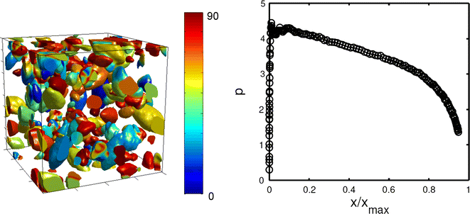

  

  Nucleation and growth of needle crystals in three dimensions, as predicted by the PBG model (Reproduced with permission from Pusztai et al.,[15] © 2005 IOP Publishing). Left: snapshot of crystallites. Different colors correspond to different orientations. Right: Avrami–Kolmogorov exponent as a function of normalized crystalline fraction

• (c) Large simulations for anisotropic growth in two dimensions (Figure 10) have led to p ≈ 3 for continuously nucleating dendritic structures.[12,28,29] This finding is attributable to a self-similar growth of squarelike equiaxed dendrites (the square is filled by secondary and higher dendrite arms and interdendritic liquid), yielding thus steady-state solidification without long-range diffusion (the solute expelled from the dendrites accumulates in the interdendritic liquid), for which indeed p = 1 + d (=3 here) applies theoretically. For a similar growth morphology but a constant number of seeds, the theoretically expected value p = d (≈2) was observed in OFPF simulations.[43]

  Fig. 10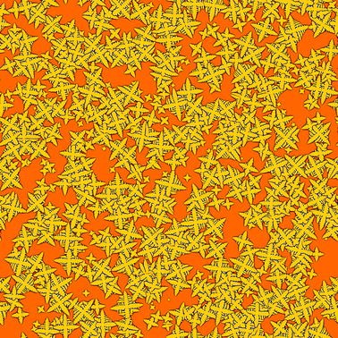

  

  Soft impingement of nucleating and growing dendrite fields in Cu-Ni at 1574 K (1301 °C), as predicted by the GPB model (Reproduced with permission from Gránásy et al.,[12] © 2002 American Physical Society). The p ≈ 3 found is consistent with nucleation and growth of impinging self-similar particles without long-range diffusion. (Computation performed on a 7000 × 7000 grid, corresponding to 92.1 μm × 92.1 μm.)

However, often the Avrami–Kolmogorov exponent deviates from these values. For example, in a 2D study of slender dendritic needle crystals[43] without secondary arms, p was found to decrease with increasing X, indicating that in this case the various level of blocking effects dominates the value of p.[43]

Another possibility is that owing to a large nucleation rate, the steady-state growth stage is not achieved for the majority of dendrites, a situation studied in three dimensions.[30,49] Then, the particles interact via their diffusion fields, in which case, in 3D handbooks,[61] expect p values falling between 2.5, corresponding to steady-state nucleation and fully diffusion-controlled growth (p = 1 + d/2), and 4.0, corresponding to steady-state nucleation and growth (p = 1 + d). Indeed such values (p = 2.99 ± 0.01[30] and p = 3.21 ± 0.01[49]) were observed in large scale simulations for multidendritic solidification (Figure 11). The larger the nucleation rate, the closer the interaction of the particles to the diffusion-controlled case. Apparently, besides reducing p, soft impingement is expected to reduce p with an extent increasing with increasing X; an expectation supported by theory[67] and PF simulations.[28] Further work is yet needed to separate the effects of anisotropy and soft impingement.

Fig. 11

Snapshot of nucleating and growing dendrites in three dimensions, as predicted by the PBG model (Reproduced with permission from Pusztai et al.,[30] © 2008 IOP Publishing). Here, a substantial fraction of the dendrites cannot reach the fully developed (steady-state) stage; thus, the Avrami–Kolmogorov exponent is p = 2.99 ± 0.01∈ [2.5,4.0]. (A 680³ grid was used in the simulation.)

Kinetics of crystallization in thin films was also investigated using the 3D version of the OFPF model.[49] The Avrami–Kolmogorov exponent observed, p = 2.37 ± 0.01,[49] falls between p = 1 + d/2 = 2.0, corresponding to steady-state nucleation and fully diffusion controlled growth, and p = 1 + d = 3.0, corresponding to steady-state nucleation and growth rates, provided that d = 2 is justifiable for thin films, an assumption valid as long as the thickness of the film is small relative to the size of the crystallites.

3.2 Columnar-to-Equiaxed Transition (CET)[70,71]

When casting alloys in a mold, the temperature increases inward and crystallization starts by heterogeneous nucleation on the walls. Due to the anisotropic growth of crystallites, grains nucleated with different orientations compete, a phenomenon leading to the selection of orientations, whose fast growth direction is essentially antiparallel with the heat flow, yielding an elongated columnar morphology.

Owing to a compositional difference between the solid and liquid phases, the solidification front is preceded by a diffusion field. This combined with an appropriate temperature gradient may lead to a region ahead of the front, where the melt is undercooled and foreign particles may induce nucleation, leading now to the formation of the equiaxed morphology that grows in the direction of heat flow. The latter phenomenon leads to the formation of small fairly uniform grain sizes. Depending on the circumstances, one may wish to enhance or eliminate CET.[71] For this, it is essential to understand the mechanism governing this phenomenon. The CET is captured fairly well by the phenomenological model of Hunt,[72] however, in terms of parameters which are difficult to quantify.

PF modeling was used to investigate the CET in two dimensions as early as 2006, however, without an orientation field.[73] In the quantitative model the authors used (incorporating antitrapping current), a few simplifications were made, such as a dilute alloy and identical crystallographic orientation being assumed for all the grains, in addition to placing the nucleation sites on a crystal lattice.

In a recent OFPF study,[58] all these simplifications were removed and quantitative computations were made for the CET in Al-Ti alloys. For this purpose, Kim’s model[56] and the PBG model[15,49] were combined, allowing us to use arbitrary thermodynamics in a quantitative model relying on the antitrapping current. The thermodynamic properties were taken from a CALPHAD assessment of the Al-Ti system.[59] Heterogeneous nucleation of the crystalline phase was approximated by the free-growth-limited model of Greer et al.[57] The foreign particles were assumed to follow a Gaussian size distribution.

As done in Reference 73, first, we have evaluated the parameters (nucleation undercooling, undercooling at the dendrite tip, and density equiaxed grains) of Hunt’s model from the simulations. Varying the pulling velocity V, and the temperature gradient G, we then performed 16 simulations: 8 above and 8 below Hunt’s curve. The results are displayed in Figure 12 for two dimensions. Apparently, the PF simulations are consistent with Hunt’s model: nucleation-controlled equiaxed structure appears for the eight runs above Hunt’s curve, whereas columnar dendritic structure is seen for the rest. Similar results were obtained in three dimensions (Figure 13).[74]

Fig. 12

Snapshot of CET, as predicted by quantitative OFPF modeling in two dimensions for an Al-Ti alloy.[58] The upper block of 16 panels shows the concentration map, whereas the lower 16 panels display the orientation field. (Different colors correspond to different orientations.) The individual panels show half of the full simulation box (0.75 mm × 0.15 mm or 1500 × 300 grid). Within the 16-panel blocks, the temperature gradient G varies as [5, 10, 20, and 40] × 10⁴  K/m from left to right, whereas the pulling velocity increases as V = [4, 8, 16, and 32] × 10⁻⁴ m/s from bottom to top. Foreign particles of Gaussian size distribution centered at 20 nm and standard deviation of 4 nm were assumed. There were (on average) ~200 foreign randomly placed particles in the simulation window. A maximum 10 pct of them were activated

Fig. 13

Equiaxed (top) and dendritic columnar (bottom) morphologies observed above and below Hunt’s analytical curve predicted by quantitative PF simulations in three dimensions for an Al-Ti alloy.[58]

3.3 Polycrystalline Growth Forms

The OFPF models achieved their most spectacular results when applied for describing exotic polycrystalline growth forms, inaccessible for other methods.

3.3.1 Disordered (“dizzy”) dendrites: particles vs M_θ

Experiments on clay-filled polymer films indicate that single crystals can be perturbed to form polycrystalline structures that are locally dendritic[19,31] via dendrite tip deflection caused by foreign particles.[41] This phenomenon was captured successfully (Figure 14) via introducing into the GPB approach an economic model of foreign particles, termed “orientation pinning centers” (areas of fixed orientation).[28,41]

Fig. 14

Disordered dendrites formed in clay-filled polymer layers (darker panels, courtesy of Vincent Ferreiro and Jack F. Douglas) and in the GPB model (lighter panels) supplemented with 18,000 orientation pinning centers (about the number of clay particles on similar area in the experiment) distributed randomly (Reproduced with permission from Gránásy et al.,[28] © 2004 IOP Publishing). The simulations differ in the initialization of the random number generator

Fig. 15

Effect of particulate additives (left two columns) and of reduced ratio χ of the orientational to translational mobility (right two columns) on the growth morphology (Reproduced with permission from Gránásy et al.,[26] © 2004 Nature Publishing Group). The first and third columns show chemical composition maps (solidus-yellow; liquidus-black), whereas the second and fourth columns display orientation maps. (Different colors stand for different crystallographic orientations.) In the left two columns, the number of orientation pinning centers varies from top to bottom as N = 0, 50,000, 200,000 and 800,000. In the right two columns, χ is multiplied by factors 1, 0.4, 0.3 and 0.1, from top to bottom. An isotropic interfacial free energy and 50 pct kinetic anisotropy of fourfold symmetry were assumed

Increasing the number of foreign particles, one can transform a single-crystal dendrite into a densely branched seaweedlike polycrystalline agglomerate of small crystallites. Such morphologies are observed for single crystals if the anisotropy is small. In our case, the anisotropy averages out along the perimeter due to the randomly oriented small crystallites. This particle-induced formation of new grains can be regarded as the heterogeneous mode of GFN.

Remarkably, a very similar effect can be seen if the orientation mobility is reduced, while keeping the PF mobility constant. Reducing M _θ , the timescale of solidification becomes too short for full orientational ordering along the perimeter of the crystal; only local ordering is possible, which leads to the formation of many differently oriented crystallites at the solidification front (Figure 15). This trapping of orientational defects into the crystalline phase offers a second homogeneous mechanism for GFN[26,28] besides the fixed angle branching enforced by cusps in f _ori[27] presented in Figure 4. While the latter is expected to prevail at both small and large anisotropies, trapping of orientational defects is expected only at high undercoolings, where for many liquids the ratio M _θ /M _ϕ ∝ χ = D _rot /D _tr decreases by orders of magnitude.[75–78]

With these three mechanisms of GFN incorporated into the GPB model, we have a flexible approach that captures an amazing variety of growth morphologies seen in laboratory and nature, including the ubiquitous spherulites.[27]

3.3.2 Spherulites

The spherulites are partly or fully (poly) crystalline, (more or less) densely branched growth morphologies (Figure 16),[21,79–89] ubiquitous under highly nonequilibrium conditions. They have an envelope roughly spherical in three dimensions (or circular in two dimensions, still retaining the name spherulite). These morphologies were observed in a broad range of materials, including pure Se;[84] oxid and metallic glasses; minerals;[88] polymers;[89] liquid crystals;[90,91] simple organic liquids;[79] fats;[92] and systems of diverse biological molecules.[93–96] Spherulitic structures were also implicated in various human diseases such as Alzheimer’s, type II diabetes, and other protein aggregation diseases.[97–99]

Fig. 16

Spherulitic morphologies (Reproduced with permission from Gránásy et al.,[27] © 2005 American Physical Society). (a) Densely branched spherulite grown in a blend of isotactic and atactic polypropylene.[80] (b) “Spiky spherulite” formed in a malonamide-d-tartatic acid mixture.[81] (c) Arboresque spherulites observed in a polypropylene film.[82] (d) and (e) “Quadrites” formed by close-to-rectangular branching in isotactic polypropylene.[24,83] (f) Spherulite in pure Se.[84] (g) Crystal sheaves found in pyromellitic dianhydrite-oxydianilin poly(imid) layer.[21] (h) Category 2 spherulites (a thin film of polybutene) with “eyes” on the two sides of the nucleation site.[85] (i) Multisheave structure observed in dilute long n-alkane blend.[86] (j) Arboresque morphology formed in polyglycine.[87] To improve the contrast, false colors were applied. The linear size of the panels is (a) 220 μm, (b) 960 μm, (c) 2.4 mm, (d) 2.5 μm, (e) 7.6 μm, (f) 550 μm, (g) 2.5 μm, (h) 20 μm, (i) 250 μm, and (j) 1.7 μm

Two main categories of the spherulitic morphologies are usually distinguished. Category 1 spherulites grow radially from their center, maintaining a space-filling character via dense branching. Category 2 spherulites are observed exclusively in systems that form needle crystals, which branch at the two ends, forming crystal “sheaves,” splaying out increasingly during growth. At longer times, the sheaves often develop “eyes” (untransformed regions) on one or both sides of the nucleation site. Ultimately, a roughly spherical (circular) growth pattern evolves, with eye structures apparent in the core region. Typical patterns observed in experimental systems[21,27,80–87] are shown in Figure 16. It was shown that this variability of the spherulitic morphology can be captured with only a handful of model parameters of the GPB model relying on the f _ori with cusps (cf. Figures 16 and 17).[27]

Fig. 17

Spherulitic morphologies by the PF theory (Reproduced with permission from Gránásy et al.,[27] © 2005 American Physical Society). The contrast of the composition maps was changed to enhance the visibility of the fine structure. The applied anisotropies have a twofold symmetry in all cases; other conditions are specified in Table II of Ref. [27]. In most cases, branching with fixed angle is the dominant GFN mechanism. Exceptions are (b), (g), and (i), where the trapping of orientational defects into the solid leads to the formation of new grains at the perimeter. Note the similarity to the experimental morphologies shown in Fig. 16

It is reassuring that the patchy nature of the orientation field that the GPB model predicts for spherulites is in remarkable agreement with the available experimental results[100,101] (Figure 18). Systematic comparison with the experiments, however, is needed to see the limitations of the model.

Fig. 18

Orientation field in Category 1 spherulites in the experiment and in the PF theory: (Left) Polarized transmission optical microscopic image of the upper half of a spherulite (Reproduced with permission from Gatos et al.,[100] © 2006 American Chemical Society). (Right) Orientation field in a PF simulation performed using the GPB model. Note the patchy nature of the orientation field in both cases

Comparable similarities between experiments and simulations can be seen in three dimensions for the Category 2 spherulites[102] and the floral spherulites[103] (Figure 19).

Fig. 19

Complex growth forms in three dimensions. (i) Category 2 spherulites in three dimensions: (a) dumbbell-shape BaCO₂ crystals (Reproduced with permission from Yu et al.,[102] © 2003 American Physical Society); (b) and (c) Qualitative PF simulations performed using the PBG model.[30] (ii) “Floral” spherulites: (d) Experimental image (Reproduced with permission from Hyde et al.,[103] © 2004 Elsevier B.V.). (e) PF simulation performed using the PBG model. It was grown from an amorphous seed (the orientation in the seed, was varied voxelwise), under parameters for which the single crystal is an extremely slender needle

3.3.3 Fractal-like polycrystals

Fractal-like aggregates are usually modeled using diffusion-limited aggregation.[104] However, as shown previously, aggregates consisting of fine crystallites can also be obtained by reducing the orientational mobility (Figure 15) in the OFPF models, while retaining coupling to the diffusive concentration field.[26] With appropriate choice of the model parameters, fractal-like polycrystalline aggregates made of very fine crystallites appear (Figure 20) that resemble closely the experimental morphologies observed, e.g., in electrodeposition.[25]

Fig. 20

Fractal-like polycrystalline growth forms as predicted by the GPB model. The chemical composition map (left) and the orientation field (right) are shown. In the latter, the liquid phase is colored black. Compare the morphology with that shown in Fig. 1(i)

3.4 Eutectic Structures

The three-field version of the OFPF model for eutectic solidification was used to address equiaxed[45] and epitaxial solidification[29] in eutectic systems. Besides the solidification morphology,[29,45] the Avrami–Kolmogorov exponent was evaluated for the equiaxed case (p ≈ 3 for steady-state nucleation, in agreement with theoretical expectations). The fourfield version (Figure 21), working with solid-liquid, solid-solid, concentration, and orientation field, was employed to model competing epitaxial and equiaxed eutectic solidification.[29] The orientation is especially important if the solid-liquid interface free energy or the kinetic coefficient is anisotropic. If, however, a single-crystal grain is considered, and the relative orientation of the crystalline phase is well defined, as often is the case, one can avoid the introduction of the orientation field. An interesting example for the latter case is the spiral eutectic dendrite shown below.

Fig. 21

Nucleation and growth of equiaxed eutectic grains in two dimensions, as predicted by the four-field OFPF model: (a) solid-liquid PF, (b) solid-solid PF, (c) concentration, and (d) orientation field. The respective Avrami–Kolmogorov exponent is p ≈ 3

3.4.1 Spiral eutectic dendrites

Recent experimental work on ternary transparent alloys indicates that owing to the pileup of the third component resulting from its different solvability in the solid and liquid phases, the flat eutectic interface becomes unstable, forming dendritic morphology, which is covered by a spiraling eutectic pattern ensuring the constant volume ratio of the two solid phases.[105] It was shown recently that a simple ternary extension of the PF model defined by Eq. [2] (however, now without f _ori) and the respective EOMs suffice to capture the essential properties of this interesting bicrystalline solidification morphology.[106] Remarkably, besides the single spiral pattern, target and multiple spiral patterns also appear (Figure 22), which do not seem to influence the shape of the eutectic dendrite. Apparently, the thermal fluctuations choose from the possible patterns, which display a peaked probability distribution,[106] a behavior analogous to the stochastic mode selection observed in helical Liesegang systems.[107]

Fig. 22

Eutectic patterns predicted for the two-phase bi- or multicrystalline dendritic structures by the ternary PF model

3.5 Manipulating the Microstructure in Thin Films

Control of the crystallization morphology is essential for various applications. Here, we briefly examine a few tools that may be used for influencing the microstructure of thin films, such as temperature oscillations, thermal gradients, spatial confinement, chemical and geometrical patterning, mechanical imprinting, or film scratching. We wish to demonstrate that PF modeling may contribute to the understanding of how these methods can be used to manipulate the microstructure.

3.5.1 Foreign particles, holes, and scratches

A straightforward idea is to use oriented/shaped particles for controlling the solidification morphology. For example, PF simulations imply that in the presence of uniformly oriented crystalline particles (represented here by orientation pinning centers of the same orientation), the dendrite arms bend so that their final crystallographic orientation coincides with that of the pinning centers (Figure 23). Further interesting possibilities are the application of orientation pinning lines and uniformly rotating orientation pinning centers: Parallel orientation pinning lines of alternating orientation lead to zigzagging dendrite arms and a striped orientation map, whereas rotating pinning centers (randomly distributed or on a lattice) lead to spiraling dendrites (Figure 24).[41]

Fig. 23

Interaction between dendrites and uniformly oriented orientation pinning centers placed on a square lattice. (Predictions by the GPB model.) The initial crystal seed had fast growth directions vertically and horizontally (orientation colored red), whereas the orientation pinning centers had a uniform orientation that has the fast growth direction rotated left by 30 deg (colored blue, on the left) or to the right with the same amount (colored yellow, on the right). Note the twisting of the dendrite arms toward the orientation forced by the pinning centers

Fig. 24

Effect of orientation pinning lines (top panels) and uniformly rotating orientation pinning centers (bottom panels) on dendritic crystallization, as predicted by the GPB model (Reproduced with permission from Gránásy et al.,[41] © 2003 Nature Publishing Group). Panels on the left show the concentration distribution, whereas on the right the orientation map is displayed

Evidently, experimental realization of such complex pinning conditions is a challenge. Suitable methods to realize them might include the use of substrate-embedded oriented particles, the rotation via an external electromagnetic field, or angular momentum control by laser pulses.[108] Early work on polymer thin films showed that nucleation can be simply achieved by piercing the film with a sharp glass fiber (Figure 25).

Fig. 25

Dendritic crystallization can easily be initiated in the polymer film in a controlled way by poking the polymer films with a glass fiber. Upper row: experiment (courtesy of Matthew L. Ferguson, who obtained the images as part of his graduate research work with Professor Wolfgang Losert, University of Maryland); central row: PF simulation, composition map; and bottom row: PF simulation, orientation map. Note that the dendrites instigated by the holes usually contain more than one orientation (normally three to five)

Extending this idea, it should be possible to print arrays of nucleation sites with specified symmetry of configuration by simply rolling a cylinder with an array of asperities over the uncrystallized polymer film, as in printing patterns on a pie crust. Such a grid of nucleation sites can be used to produce an ordered array of spherulites (Figure 26). It is expected that the orientation of the nucleation points could be controlled by making the asperities in the form of flat pins of controlled orientation. In this way, it should be possible to create a wide range of crystallization morphologies and to tune the topography, permeability, and mechanical properties of the crystallized polymer film. These orientation-controlling techniques may open a new route for tailoring solidification microstructures.

Fig. 26

Spherulitic solidification on patterned substrate. Left and middle: PF simulation of spherulites arranged into a 5 × 5 square-grid array. Part of the chemical composition and orientation maps rotated by 45 deg to match the experiment. Right: the experimental image shows a small 3 × 3 array or early stage PEO spherulites formed by indenting and then crystallizing a polymer film (courtesy of Brian C. Okerberg)

Experience shows that scratches in polymer layers appear to be heterogeneous nucleation sites rather than orientation pinning lines. Accordingly, they can be represented by appropriate boundary conditions setting the contact angle in the PF simulations.[30,39,40] Snapshots of a simulation performed with a contact angle of 10 deg are shown in Figure 27. Scratching suitably the polymer film offers a way to orient the dendrites covering a surface.

Fig. 27

Dendritic growth originating from a scratch in a polymer film of the PS/PVME polymer mater discussed (left panel, courtesy of Vincent Ferreiro). A PF simulation with serrated scratch edges (characterized by 10 deg contact angle) is shown in the central and right panels (displaying the composition and orientation maps, respectively). Note that the symmetry breaking effect of film scratching induces the dendrite to orient nearly perpendicularly to the scratch

3.5.2 Temperature gradient

Experiments indicate[109,110] that distorted spherulites appear under the influence of the temperature gradient on nucleation and growth kinetics, resulting in a “shooting star” morphology. This type of morphology can readily be described by PF simulations that incorporate a temperature gradient (Figure 28). Such temperature gradients are prevalent in the manufacture of semicrystalline polymeric materials, offering an opportunity for property control.

Fig. 28

Spherulites grown in the temperature gradient in the experiment (left (Reproduced with permission from Pawlak et al.,[109] © 2001 Springer Publishing)) and in the PF theory (right). Note the “shooting star” morphology, characteristic to this scenario

3.5.3 Crystallization in confined domains

Development of boundary conditions,[30,39,40] which realize walls of controlled properties such as contact angle and local crystallographic properties (glassy, single- or polycrystalline), enabled us to define various types of heterogeneities within the PF theory, including particles or containers of complex shape. Using these techniques, one may investigate whether the orientation selector (“pigtail”) employed for producing single-crystal casting can be used to get rid of spherulitic crystallization. Whereas in the case of dendritic solidification of the many crystal orientations present initially only a single orientation survives in the meandering channel, leading to single-crystal freezing in the cast volume (Figure 29(a)),[28] due to GFN (an inherent interfacial property of this growth mode), polycrystalline growth propagates through the orientation selector, initiating spherulitic growth inside the cast volume (Figure 29(b)).[111] Indeed, the latter prediction was confirmed by recent experiments on organic thin films[112] (Figure 29(c), (d)).

Fig. 29

Crystallization in rectangular channels: PF simulations (a) for dendritic[28] and (b) spherulitic[111] solidification in a 2D orientation selector (pigtail). The orientation field is shown (different colors correspond to different orientations, white-mold). In the case of dendritic solidification, crystallization starts on the left with several crystallographic orientations, but only a single crystallographic orientation survives the meandering channel. This, however, does not stand for the spherulites, where GFN cannot be disabled by the orientation selector. (c), (d) spherulitic crystallization of organic thin film in a rectangular channel (Reproduced with permission from Lee et al.,[112] © 2012 John Wiley & Sons). The polycrystalline nature of spherulitic growth is retained throughout the growth in the channel as predicted by the PF simulation shown in panel (b)

The same boundary conditions can be used to define tubes for modeling the formation of polymeric shish-kebab structures[113] on carbon nanotubes (Figure 30).[40]

Fig. 30

Polymeric shish-kebab structure formed on carbon nanotubes. Left and middle: experiment (Reproduced with permission from Li et al.,[113] © 2005 John Wiley & Sons); right: OFPF simulation using the PBG model (Reproduced with permission from Warren et al.,[40] © 2009 American Physical Society)

3.5.4 Time-dependent external field

There is a great deal of interest in how temporal variations in processing conditions (temperature, pressure, etc.) influence the crystallization morphology and the ultimate properties of the resulting materials.[79,80,114–116] For example, PF simulations for dendritic solidification under oscillating pressure or temperature predict that the frequency of side branching of the dendrite can be tuned by the frequency of the external forcing,[115,116] a phenomenon confirmed by experiments on liquid crystals.[115,116] Periodic laser pulses were also used to control solidification morphology and grain boundary dynamics in polycrystalline matter.[117–120]

The oscillating temperature was used for controlling the crystallization morphology in polymer films, which was made to alternate between a fractal-like seaweed front and a smooth front. Here, seaweed morphology forms due to a diffusional-instability-driven fingering at the higher temperature, whereas diffusionless growth with a smooth interface takes place at the lower limiting temperature. The latter morphology is made possible by a reduction of growth anisotropy of crystal growth due to kinetic roughening occurring at large undercooling, which leads to interface broadening. Switching between these two growth modes, via oscillating the temperature, leads to a concentric ring structure both in experiment and in PF simulations, when starting from a crystalline seed (Figure 31).

Fig. 31

Concentric seaweed and smooth-front regions emerging from alternating diffusion-controlled and diffusionless growth mechanisms induced by oscillating (homogeneous) temperature (a) in a polymer thin film (courtesy of Vincent Ferreiro) and (b) in a PF simulation. These are single-crystal objects. It is remarkable that very similar morphologies (fractal-like seaweed) may exist in single crystalline (here) and in polycrystalline forms (cf. Fig. 20)

4 Summary and Closing Remarks

We reviewed the advances made in the orientation-field-based PF models during the past decade. These models have contributed to the understanding of phenomena governing the formation of complex polycrystalline structures including multidendritic patterns, CET, dendrites disordered by foreign particles, spherulites, fractal-like aggregates, and spiraling eutectic dendrites. They seem to be useful in gaining understanding of how one may govern microstructure via perturbing solidification.

Unsolved problems and future challenges: While one of the advantages of the OFPF models relative to the MPF models is that a more complete picture of grain boundary dynamics is provided, including the possibility for grain rotation seen in experiments,[121–124] recent studies[46,125] point out that the simple relaxation equation for the orientation field used by the OFPF models is not entirely consistent with the coherent crystalline structure of matter: unlike liquid crystals (for which relaxation dynamics would be more appropriate), a crystal is not free to change its local orientation to lower the free energy. The assumed relaxation dynamics of the orientation field sometimes lead to predictions that are qualitatively wrong. For example, in the case of a circular grain embedded into an infinite crystal, the OFPF models predict homogeneous grain rotation that reduces the orientational differences. In contrast, atomistic studies show that the inner crystal performs a rigid body rotation away from the orientation of the outer crystal, due to geometrical constraints on the dislocations.[126] Although the committed errors are probably small for large-scale grain structures, this needs to be confirmed in each case. It is appropriate to note, however, that these problems refer to the predicted long-term grain boundary dynamics, whereas in the majority of the OFPF studies addressing polycrystalline solidification, a vanishing orientational mobility was used inside the solid, so the respective results are not affected. Indeed, “in the interfacial region where the structure of the solid in not yet fully established, the concept of rotational mobility is valid.”[125]

A further weak point of PF/OFPF simulations is crystal nucleation, a phenomenon that appears to be more complex than anticipated previously (for example, a two-step precursor-mediated process seems fairly general[127–131]).

Most of the OFPF simulations reviewed here are qualitative. Exceptions are, as mentioned previously, the OFPF simulations describing CET in Al-Ti alloys (polycrystalline structures of Class I).[58] Further work is needed to extend quantitative PF modeling to polycrystals of Classes II and III. Besides the difficulties already mentioned in Section II–C, it is usually a considerable challenge to extend quantitative predictions to new classes of materials. While on the modeling side appropriate theoretical tools are available, and the ever-increasing computational power is an enormous help, sufficiently detailed information on the material properties needed as input for the PF models is available only for relatively few classes of materials (e.g., metallic alloys). What one needs is thermodynamic data for all the phases, diffusion coefficients, and interface free energies (solid-liquid and solid-solid), with their respective anisotropies. While in many cases databases provide the required thermodynamic and diffusion data (Thermo-Calc,[132] ChemSage,[133] FactSage,[134] DICTRA,[135] etc.), little is known usually of the interfacial properties, including the magnitude and anisotropy of the interface-free energies and the kinetic coefficient. Information on the latter properties comes dominantly from atomistic simulations that are as good as the empirical model potential applied and are often in contradiction with the best experimental data. As a result, the extension of quantitative simulations for further classes of materials requires a concerted effort of groups of scientists. Large international projects may provide the required logistics.

Further efforts are needed to incorporate elasticity and fluid flow in a way consistent with the orientation field, yet allowing the rigid body motion of individual dendrites.

It remains to be seen how much the combination of advanced numerical methods (adaptive grid + implicit schemes) can improve the efficiency of OFPF codes. Adaptation of such methods for the OFPF models is often not immediately straightforward, especially when the thermal fluctuations are considered: coarse graining of the orientation field raises specific issues associated with the averaging of angles.

Finally, we note that the present OFPF approaches contain heuristic elements. Recent developments in the area of atomistic continuum approaches (e.g., the Phase-Field Crystal model (for a review, see Reference 136) or PF models based on the cluster variation method[137]) offer new possibilities to deduce physically motivated models for polycrystalline solidification and a remedy for some of the problems mentioned here.

References

J. J. Hoyt, M. Asta, and A. Karma: Mater. Sci. Eng. R, 2003, vol. 41, pp. 121–63.
A. Karma and W.-J. Rappel: Phys. Rev. E, 1998, vol. 57, pp. 4323–49.
J. Bragard, A. Karma, Y.H. Lee, and M. Plapp: Interf. Sci., 2002, vol. 10, pp. 121–36.
I. Steinbach, E. Pezzolla, B. Nestler, J. Rezende, M. Seesselberg, and G.J. Schmitz: Physica D, 1996, vol. 94, pp. 135–47.
D. Fan and L.-Q. Chen: Acta Mater., 1997, vol. 45, pp. 611 – 22.
N. Moelans, B. Blanpain, and P. Wollants: Phys. Rev. B, 2008, vol. 78, art. no. 024113.
N. Moelans, B. Blanpain, and P. Wollants: Phys. Rev. Lett., 2008, vol. 101, art. no. 025502.
N. Moelans, F. Wendler, and B. Nestler: Comput. Mater. Sci., 2009, vol. 46, pp. 479–90.
L.-Q. Chen: Annu. Rev. Mater. Res., vol. 32. pp. 113–40.
R. Kobayashi, J.A. Warren, and W.C. Carter: Physica D, 1998, vol. 119, pp. 415–23.
J.A. Warren, R. Kobayashi, A.E. Lobkovsky, and W.C. Carter: Acta Mater., 2003, vol. 51, pp. 6035–58.
L. Gránásy, T. Börzsönyi, and T. Pusztai: Phys. Rev. Lett., 2002, vol. 88, art. no. 206105.
L. Gránásy, T. Börzsönyi, and T. Pusztai: in Interface and Transport Dynamics, Computational Modelling, H. Emmerich, B. Nestler, and M. Schreckenberg, eds., Lecture Notes in Computational Science and Engineering, Springer, Berlin, 2003, vol. 32, pp. 190–95.
R. Kobayashi and J.A. Warren: TMS Lett., 2005, vol. 1, pp. 1–2.
T. Pusztai, G. Bortel, and L. Gránásy: Europhys. Lett., 2005, vol. 71, pp. 131–37.
L. Gránásy, T. Pusztai, T. Börzsönyi, G.I. Tóth, G. Tegze, J.A. Warren, and J.F. Douglas: Philos. Mag., 2006, vol. 86, pp. 3757–78.
K. Lee and W. Losert: personal communication, University of Maryland, Maryland, 2004.
B.D. Nobel and P.F. James: personal communication, University of Sheffield, Sheffield, 2003.
V. Ferreiro, J.F. Douglas, J.A. Warren, and A. Karim: Phys. Rev. E, 2002, vol. 65, art. no. 051606.
G. Ryschenkow and G. Faivre: J. Cryst. Growth, 1988, vol. 87, pp. 221–35.
M. Ojeda and D.C. Martin: Macromolecules, 1993, vol. 26, pp. 6557–65.
F.J. Padden and H.D. Keith: J. Appl. Phys., 1965, vol. 36, pp. 2987–95.
H.D. Keith, F.J. Padden, Jr., and R.G. Vadimsky: J. Polym. Sci. Part A-2, 1966, vol. 4, pp. 267–81.
F. Khoury: J. Res. Nat. Bur. Stand. A, 1966, vol. 70, pp. 29–61.
V. Fleury: Nature, 1997, vol. 390, pp. 145–48.
L. Gránásy, T. Pusztai, T. Börzsönyi, J.A. Warren, and J.F. Douglas: Nat. Mater., 2004, vol. 3, pp. 645–50.
L. Gránásy, T. Pusztai, G. Tegze, J.A. Warren, and J.F. Douglas: Phys. Rev. E, 2005, vol. 72, art. no. 011605.
L. Gránásy, T. Pusztai, and J.A. Warren: J. Phys.: Condens. Matter, 2004, vol. 12, pp. R1205–R1235.
L. Gránásy, T. Pusztai, and T. Börzsönyi: in Handbook of Theoretical and Computational Nanotechnology, M. Rieth and W. Schommers, eds., American Science Publishers, Stevenson Ranch, CA, 2006, vol. 9, pp. 525–72.
T. Pusztai, G. Tegze, G. I. Tóth, L. Környei, G. Bansel, Z. Fan, and L. Gránásy: J. Phys.: Condens. Matter, 2008, vol. 20, art. no. 404205.
V. Ferreiro, J.F. Douglas, J.A. Warren, and A. Karim: Phys. Rev. E., 2002, vol. 65, art. no. 042802.
B. Morin, K.R. Elder, M. Sutton, and M. Grant: Phys. Rev. Lett., 1995, vol. 75, pp. 2156–59.
J.A. Warren, R. Kobayashi, and W.C. Carter: J. Cryst. Growth, 2000, vol. 211, pp. 18–20.
R. Kobayashi, J.A. Warren, and W.C. Carter: Physica D, 2000, vol. 140, pp. 141–50.
A.E. Lobkovsky and J.A. Warren: Phys. Rev. E, 2001, vol. 63, art. no. 051605.
R. Kobayashi and Y. Giga: J. Stat. Phys., 1999, vol. 95, pp. 1187–1220.
J.A. Warren and W.J. Boettinger: Acta Metall. Mater., 1995, vol. 43, pp. 689–703.
J.W. Cahn and J.E. Hilliard: J. Chem. Phys., 1959, vol. 31, pp. 688–99.
L. Gránásy, T. Pusztai, D. Saylor, and J.A. Warren: Phys. Rev. Lett., 2007, vol. 98, art. no. 035703.
J.A. Warren, T. Pusztai, L. Környei, and L. Gránásy: Phys. Rev. B, 2009, vol. 79, art. no. 014204.
L. Gránásy, T. Pusztai, J.A. Warren, J.F. Douglas, T. Börzsönyi, and V. Ferreiro: Nat. Mater., 2003, vol. 2, pp. 92–96.
L. Gránásy, T. Pusztai, T. Börzsönyi, G. Tóth, G. Tegze, J.A. Warren, and J.F. Douglas: J. Mater. Res., 2006, vol. 21, pp. 309–19.
J.J. Li, J.C. Wang, Q. Xu, and G.C. Yang: Acta Mater., 2007, vol. 55, pp. 825–32.
M. Asanishi, T. Takaki, and Y. Tomita: Proc. ATEMA 2007, Montreal, Advanced Engineering Solutions, Ottawa, 2007, pp. 195–203.
D. Lewis, T. Pusztai, L. Gránásy, J. Warren, and W. Boettinger: JOM, 2004, vol. 56, pp. 34–39.
H. Henry, J. Mellenthin, and M. Plapp: Phys. Rev. B, 2012, vol. 86, art. no. 054117.
J. Mellenthin: Ph.D. Thesis, École Polytechnique, Palaiseau, France, 2007.
G.A. Korn and T.M. Korn: Mathematical Handbook for Scientists and Engineers, McGraw-Hill, New York, NY, 1970, ch. 14.10.
T. Pusztai, G. Bortel, and L. Gránásy: Proc. Modeling of Casting, Welding and Advanced Solidification Processes-XI, C.-A. Gandin and M. Bellet, eds., TMS, Warrendale, PA, 2006, pp. 409–16.
M. Asta, J.J. Hoyt, and A. Karma: Mater. Sci. Eng. R, 2003, vol. 41, pp. 121–63.
F. Podmaniczky, G.I. Tóth, T. Pusztai, and L. Gránásy: J. Cryst. Growth. DOI:10.1016/j.jcrysgro.2013.01.036.
M. Dorr, J.L. Fattebert, M.E. Wickett, J.F. Belak, P.E.A. Turchi: J. Comput Phys., 2010, vol. 229, pp. 626–41.
T. Pusztai and L. Gránásy: unpublished research.
R. Kobayashi and J.A. Warren: Physica A, 2005, vol. 356, pp. 127–32.
A. Karma: Phys. Rev. Lett, 2001, vol. 87, art. no. 115701.
S.G. Kim: Acta Mater., 2007, vol. 55, pp. 4391–99.
A.L. Greer, A.M. Brunn, A. Tronche, P.V. Evans, and D.J. Bristow: Acta Mater., 2000, vol. 48, pp. 2823–35.
Work performed within EU FP6 Integrated Project, NMP3-CT-2004-500635, Intermetallic Materials Processing in Relation to Earth and Space Solidification (IMPRESS), 2004–2009, http://spaceflight.esa.int/impress/.
V.T. Witusiewicz, A.A. Bondar, U. Hecht, S. Rex, and T.Y. Velikanova: J. Alloys Compd., 2008, vol. 465, pp. 64–77.
http://spaceinvideos.esa.int/Videos/2012/07/Kaleidoscopic_nanocomposite_metals.
J.W. Christian: The Theory of Transformations in Metals and Alloys, Pergamon, Oxford, U.K., 1981.
J.W. Cahn: Mater. Res. Soc. Symp. Proc., 1996, vol. 398, pp. 425–37.
D.P. Birnie III and M.C. Weinberg: J. Chem. Phys., 1995, vol. 103. pp. 3742–46.
B.J. Kooi: Phys. Rev. B, 2004, vol. 70, art. no. 224108.
M.P. Shepilov and D.S. Baik: J. Non-Cryst. Solids, 1994, vol. 171, pp. 141–56.
T. Pusztai and L. Gránásy: Phys. Rev. B, 1998, vol. 57, pp. 14110–18.
T. Pradell, D. Crespo, N. Clavaguera, and M.T. Clavaguera-Mora: J. Phys.: Condens. Matter, 1998, vol. 10, pp. 3833–44.
M.T. Clavaguera-Mora, N. Clavaguera, D. Creaspo, and T. Pradell: Progr. Mater. Sci., 2002, vol. 47, pp. 559–619.
M. Tomellini: Comput. Mater. Sci., 2010, vol. 50, pp. 2371–79.
W. Kurz and D.J. Fisher: Fundamentals of Solidification, Trans Tech Publications, Lausanne, 1989, pp. 1–20.
W. Kurz, C. Bezencon, and M. Gaumann: Sci. Technol. Adv. Mater., 2001, vol. 2, pp. 185–91.
J.D. Hunt: Mater. Sci. Eng., 1984, vol. 65, pp. 75–83.
A. Badillo and C. Beckermann: Acta Mater., 2006, vol. 54, pp. 2015–16.
E. Rössler: Phys. Rev. Lett., 1990, vol. 65, pp. 1595-98.
I. Chang and H. Sillescu: J. Phys. Chem. B, 1997, vol. 101, pp. 8794-8801.
M.D. Ediger: Ann. Rev. Phys. Chem., 2000, vol. 51, pp. 99-128.
K.L. Ngai, J.H. Magill, and D.J. Plazek: J. Chem. Phys., 2000, vol. 112, pp. 1887-92.
J.H. Magill and D.J. Plazek: J. Chem. Phys., 1967, vol. 46, pp. 3757–69.
H.D. Keith and F.J. Padden: J. Appl. Phys., 1964, vol. 35, pp. 1270–85.
H.D. Keith and F.J. Padden: J. Appl. Phys., 1963, vol. 34, pp. 2409–21.
M.L. Walker, A.P. Smith, and A. Karim: Langmuir, 2003, vol. 19, pp. 6582–85.
B. Lotz and J.C. Wittmann: J. Polym. Sci., Part B: Polym. Phys., 1986, vol. 24, pp. 1541–58.
G. Ryschenkow and G. Faivre: J. Non-Cryst. Solids, 1988, vol. 87, pp. 221–35.
P.H. Geil: Polymer Single Crystals, Wiley, New York, NY, 1963.
L. Hosier, D.C. Bassett, and A.S. Vaughan: Macromolecules, 2000, vol. 33, pp. 8781–90.
C.A. Self and C.A. Hill: J. Cave Karst Studies, 2003, vol. 65, pp. 130–51.
J.H. Magill: J. Mater. Sci., 2001, vol. 36, pp. 3143–64.
J.L. Hutter and J. Bechhoefer: Phys. Rev. E, 1999, vol. 59, pp. 4342–52.
J.L. Hutter and J. Bechhoefer: J. Cryst. Growth, 2000, vol. 217, pp. 332–43.
A.G. Marangoni and M. Ollivon: Chem. Phys. Lett., 2007, vol. 442, pp. 360–64.
D. Lomas, D.L. Evans, J.T. Finch, and R.W. Carell: Nature, 1992, vol. 357, pp. 605–07.
E.H. Koo, P.T. Lansbury, and J.W. Kelly: PNAS, 1993, vol. 96, pp. 9989–90.
L.-W. Jin, K.A. Claborn, M. Kurimoto, M.A. Geday, I. Maezawa, F. Sohraby, M. Estrada, W. Kaminsky, and B. Kahr: PNAS, 2003, vol. 100, pp. 15294–98.
M.R.H. Krebs, C.E. MacPhee, A.F. Miller, I.E. Dunlop, C.M. Dobson, and A.M. Donald: PNAS, 2004, vol. 101, pp. 14420–24.
S.S. Rogers, M.R.H. Krebs, E.H.C. Bromley, E. van der Linden, and A.M. Donald: Biophys. J., 2006, vol. 90, pp. 1043–54.
K.R. Domike and A.M. Donald: Int. J. Biol. Macromol., 2009, vol. 44, pp. 301–10.
C. Exley, E. House, J.F. Collingwood, M.R. Davidson, D. Cannon, and A.M. Donald: J. Alzheimers Dis., 2010, vol. 20, pp. 1159–65.
K.G. Gatos, C. Minogianni, and C. Galiotis: Macromolecules, 2006, vol. 40, pp. 786–89.
E. Gunn, L. Wong, C.W. Branham, B. Marquardt, and B. Kahr: Cryst. Eng. Comm., 2011, vol. 13, pp. 1123–26.
S.-H. Yu, H. Cölfen, and M. Antonietti: J. Phys. Chem. B, 2003, vol. 107, pp. 7396–7405.
S.T. Hyde, A.M. Carnerup, A.-K. Larsson, A.G. Christy, and J.M. Garcia-Ruiz: Physica A, 2004, vol. 339, pp. 24–33.
T.A. Witten, Jr. and L.M. Sander: Phys. Rev. Lett., 1981, vol. 47, pp. 1400–03.
S. Akamatsu, M. Perrut, S. Bottin-Rousseau, and G. Faivre: Phys. Rev. Lett., 2010, vol, 104, art. no. 056101.
T. Pusztai, L. Rátkai, A. Szállás, and L. Gránásy: Phys. Rev. E, 2013, vol. 87, art. no. 032401.
S. Thomas, I. Lagzi, F. Molnár, and Z. Rácz: Phys. Rev. Lett., 2013, vol. 110, art. no. 078303.
L. Allen, M.W. Beijersbergen, R.J.C. Spreeuw, and J.P. Woerdman: Phys. Rev. A, 1992, vol. 45, pp. 8185–89.
A. Pawlak and E. Piorkowska: Coll. Polym. Sci., 2001, vol. 279, pp. 939–46.
C. Charbon and S. Swaminarayan: Polym. Eng. Sci., 1998, vol. 38, pp. 634–56.
Simulation performed by L. Gránásy and T. Pusztai in Oct. 2005; presented in invited talk “Growth and Form of Spherulites: A Phase Field Study,” L. Gránásy, T. Pusztai, G. Tegze, G. Bortel, J.A. Warren, and J.F. Douglas, eds., APS March Meeting, Baltimore, MD, Mar. 13–16, 2006.
S.S. Lee, S.B. Tang, D.-M. Smilgies, A.R. Woll, M.A. Loth, J.M. Mativetsky, J.E. Anthony, and Y.-L. Loo: Adv. Mater., 2012, vol. 24, pp. 2692–98.
C.Y. Li, L. Li, W. Cai, S.L. Kodjie, and K.K. Tenneti: Adv. Mater., 2005, vol. 17, pp. 1198–1202.
L. Williams, M. Muschol, X. Qian, W. Losert, and H.Z. Cummins: Phys. Rev. E, 1993, vol. 48, pp. 489–99.
T. Börzsönyi, T. Tóth-Katona, Á. Buka, and L. Gránásy: Phys. Rev. Lett., 1999, vol. 83, pp. 2853–56.
T. Börzsönyi, T. Tóth-Katona, Á. Buka, and L. Gránásy: Phys. Rev. E, 2000, vol. 62, pp. 7817–27.
M. Fell and J. Bilgram: Phys. Rev. E, 2007, vol. 75, art. no. 061603.
K. Lee and W. Losert: J. Cryst. Growth, 2004, vol. 269, pp. 592–98.
K. Lee and W. Losert: Acta Mater., 2005, vol. 53, pp. 3503–10.
A.J. Pons, A. Karma, S. Akamatsu, M. Newey, A. Pomerance, H. Singert, and W. Losert: Phys. Rev. E, 2007, vol. 75, art. no. 021602.
J.W. Cahn and J.E. Taylor: Acta Mater., 2004, vol. 52, pp. 4887–98.
J.W. Cahn, Y. Mishin, and A. Suzuki: Philos. Mag., 2006, vol. 86, pp. 3965–80.
S.G. Srinivasan and J.W. Cahn: in Science and Technology of Interfaces, S. Ankem, C.S. Pande, I. Ovidko, and S. Ranganathan, eds., TMS, Seattle, WA, 2002, pp. 3–14.
M. Upmanyu, D.J. Srolovitz, A.E. Lobkovsky, J.A. Warren, and W.C. Carter: Acta Mater., 2006, vol. 54, pp. 1707–19.
M. Plapp: Philos. Mag., 2011, vol. 91, pp. 25–44.
K.-A. Wu and P.W. Voorhees: Acta Mater., 2012, vol. 60, pp. 407–19.
J.F. Lutsko and G. Nicolis: Phys. Rev. Lett., 2006, vol. 96, art. no. 046102.
T. Schilling, H.J. Schöpe, M. Oettel, G. Opletal, and I. Snook: Phys. Rev. Lett., 2010, vol. 105, art. no. 025701.
G.I. Tóth, T. Pusztai, G. Tegze, G. Tóth, and L. Gránásy: Phys. Rev. Lett., 2011, vol. 107, art. no. 175702.
G.I. Tóth, G. Tegze, T. Pusztai, and L. Gránásy: Phys. Rev. Lett., 2012, vol. 108, art. no. 022502.
T. Kawasaki and H. Tanaka: PNAS, 2010, vol. 107, pp. 14036–41.
Thermo-Calc Software: http://www.thermocalc.com.
ChemSage software: http://gtt.mch.rwth-aachen.de/gtt-web/chemsage.
FactSage software: http://www.factsage.com//.
DICTRA software: http://www.thermocalc.com/DICTRA.htm/.
H. Emmerich, H. Löwen, R. Wittkowski, T. Gruhn, G.I. Tóth, G. Tegze, and L. Gránásy: Adv. Phys., 2012, vol. 61, pp. 665–743.
For a review, see T. Mohri: in Alloy Physics: A Comprehensive Reference, W. Pfeiler, ed., Wiley-VCH Verlag GmbH & Co. KGaA, Weinheim, 2007, pp. 525–88.
Acknowledgments
We thank James A. Warren (NIST) and Jack F. Douglas (NIST) for the enlightening discussions during the early works, and Jack F. Douglas for calling our attention to different interesting possibilities that influence crystallization morphology. We also thank Vincent Ferreiro, Brian C. Okerberg, and Matthew L. Ferguson for providing images of crystallizing polymers. This review includes techniques developed in the framework of the EU FP7 Collaborative Project “EXOMET” (Contract No. NMP-LA-2012-280421, co-funded by ESA) and ESA MAP/PECS projects “MAGNEPHAS III” (Contract No. 4000105034/11/NL/KML) and “GRADECET” (Contract No. 4000104330/11/NL/ KML).
Author information
Authors and Affiliations
Corresponding author
Additional information
Manuscript submitted May 7, 2013.
Rights and permissions
About this article
Cite this article
Gránásy, L., Rátkai, L., Szállás, A. et al. Phase-Field Modeling of Polycrystalline Solidification: From Needle Crystals to Spherulites—A Review. Metall Mater Trans A 45, 1694–1719 (2014). https://doi.org/10.1007/s11661-013-1988-0
Published:
Issue Date:
DOI: https://doi.org/10.1007/s11661-013-1988-0