Ringel duality for certain strongly quasi-hereditary algebras

Abstract

We study quasi-hereditary endomorphism algebras defined over a new class of finite dimensional monomial algebras with a special ideal structure. The main result is a uniform formula describing the Ringel duals of these quasi-hereditary algebras. As special cases, we obtain a Ringel duality formula for a family of strongly quasi-hereditary algebras arising from a type A configuration of projective lines in a rational, projective surface as recently introduced by Hille and Ploog, for certain Auslander–Dlab–Ringel algebras, and for Eiriksson and Sauter’s nilpotent quiver algebras when the quiver has no sinks and no sources. We also recover Tan’s result that the Auslander algebras of self-injective Nakayama algebras are Ringel self-dual.

1 Introduction

Quasi-hereditary algebras form an important class of finite dimensional algebras with relations to Lie theory (this was the original motivation [10]) and exceptional sequences in algebraic geometry (see e.g. [9, 23]). Examples of quasi-hereditary algebras include blocks of category and Schur algebras.

Ringel duality [34] is a fundamental phenomenon in the theory of quasi-hereditary algebras, see for example [8, 13,14,15, 19, 22, 26, 28, 33] for (recent) work on this topic. For any quasi-hereditary algebra A there exists a quasi-hereditary algebra $\mathfrak {R}(A)$, the Ringel dual of A, such that

$$\begin{aligned} A\text {-mod} \cong \mathfrak {R}(\mathfrak {R}(A))\text {-mod}. \end{aligned}$$

However, computing the Ringel dual of a quasi-hereditary algebra explicitly may not be straightforward. In this paper we introduce a new class of quasi-hereditary algebras that admit a uniform description of their Ringel duals, see Theorem 1.2.

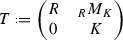
Let us make this more precise. Let k be an algebraically closed field, and R be a finite dimensional monomial k-algebra, i.e. $R=kQ/I$, where I is a two-sided ideal generated by paths in Q. For example , where I is a two-sided ideal generated by monomials in .

Definition 1.1

We call R ideally ordered, if for every primitive idempotent $e \in R$ and every pair of monomials $m, n \in eR$ there exists an epimorphism $Rm \rightarrow Rn$ or an epimorphism $Rn \rightarrow Rm$.

For an algebra R we consider the additive subcategory of all torsionless R-modules

define to be the direct sum of all indecomposable modules in up to isomorphism, and set

For submodules $\Lambda \subset R$ we define the layer function and we call l the ideal layer function. For an ideally ordered algebra R the isomorphism classes of submodules $\Lambda \subset R$ label the simple modules $S(\Lambda )$ of and so the ideal layer function induces a partial ordering on the simple -modules: $S(\Lambda _1) \leqslant S(\Lambda _2)$ $\Leftrightarrow$ $l(\Lambda _1) \leqslant l(\Lambda _2)$. We call this the ideal layer ordering.

The following is the main result of this paper and calculates the Ringel dual for algebras of the form . See Theorem 5.1 for a more detailed version.

Theorem 1.2

Let R be a finite dimensional ideally ordered monomial algebra. Then is quasi-hereditary with respect to the ideal layer ordering, has global dimension $\leqslant 2$, and has Ringel dual $E_{R^{\mathrm{op}}}^{\mathrm{op}}$:

Remark 1.3

As we were preparing to post this paper on the arXiv we became aware of the very recent paper [14] of Coulembier that had just appeared. This paper introduces a more general version of the Auslander–Dlab–Ringel construction and proves a Ringel duality formula in this setting. In particular, this generalises the Ringel duality formula of Conde and Erdmann [13] that we discuss below.

Our construction appears to be a special case that fits into this more general framework which, in particular, implies the Ringel duality formula of Theorem 1.2. However, the approach and proof in Coulembier’s work is different to the one in this paper. The work of Coulembier also seems to answer the questions we raise in Remark 5.3 (1) and at the end of Sect. 6.3 regarding the possibility of finding a more general framework in which a Ringel duality formula holds.

In light of this, the results of this paper can be thought of as providing a very explicit example of Coulembier’s Ringel duality formula, linking to several geometrically inspired examples such as Knörrer invariant algebras, and proving further properties that hold in our special case of the algebras such as being simultaneous left and right strongly quasi-hereditary for the same quasi-hereditary order and being left ultra strongly quasi-hereditary.

The class of ideally ordered monomial algebras includes many well known examples, and in many of these examples the endomorphism algebras $E_{R}$ are also well understood.

Example 1.4

The following families of finite dimensional monomial algebras are ideally ordered.

• (0) Hereditary algebras.

• (1) The algebras for positive integers l, m.

• (2) More generally, for Q a finite quiver, $J \subseteq kQ$ the two-sided ideal generated by all arrows in Q, and $m \geqslant 0$ the algebra is ideally ordered.

  To prove this, consider a monomial $p \in eR$. There is a surjection $Re \rightarrow Rp$ given by $g \mapsto gp$ with kernel

  

  where i is minimal such that $p \in J^i$. Hence for any monomial $p \in eR$ there is an isomorphism $Rp \cong Re/J^le$ for some . As a result, for any pair of monomials $p,q \in eR$ the monomial ideals Rp, Rq are isomorphic to some pair of quotient modules occurring in the chain of surjections

  $$\begin{aligned} Re \cong Re/J^{m}e \rightarrow Re/J^{m-1}e \rightarrow \cdots \rightarrow Re/J^{1}e. \end{aligned}$$

  Hence there is a surjection $Rp \rightarrow Rq$ or $Rq \rightarrow Rp$.

• (3) For every pair $0<a<r$ of coprime integers the finite dimensional monomial Knörrer invariant algebra $K_{r,a}$ is defined in [27, Definition 4.6], and the results of [27, Section 6.4] describe its monomial ideals and imply that it is ideally ordered. The definition of these algebras is recapped in Sect. 6.1.

• (4) Nakayama algebras, introduced in [31], are ideally ordered.

We give two constructions that can be used to produce ideally ordered monomial algebras.

• (5) Let R and K be ideally ordered monomial algebras and let $_R M_K$ be an R-K-bimodule which is projective as R-module and as K-module. Then

  

  is an ideally ordered monomial algebra. Example 2.8 (a) shows that T need not be ideally ordered if we weaken the assumptions on $_R M_K$.

• (6) If R is ideally ordered and $e \in R$ is an arbitrary idempotent, then eRe is ideally ordered.

  Suppose that $f \in eRe$ is a primitive idempotent and $p,q \in feRe=fRe$ are monomials. Then f is a primitive idempotent in R, $p,q \in fR$ are monomials, and as R is ideally ordered there is a surjection between Rp and Rq. Applying

  

  to this surjection of R-modules will produce the required surjection of eRe-modules between eRp and eRq since is exact. This shows eRe is ideally ordered.

We finish by exhibiting a local commutative monomial algebra which is not ideally ordered.

• (7) The algebra is not ideally ordered. To see this consider the ideals Rx and Ry.

We briefly discuss how these examples of ideally ordered monomial algebras R, and the algebras they define, relate to algebras and results in the literature.

1.1 Hille and Ploog’s algebras

The Ringel duality formula of Theorem 1.2, the definition of ideally ordered monomial algebras, and the construction of the algebras in this paper are all geometrically inspired. They were first observed in our previous work [27] for a class of quasi-hereditary algebras $\Lambda _\alpha$ constructed by Hille and Ploog [24].

In more detail, the algebras $\Lambda _{\varvec{\alpha }}$ arise from an exceptional collection of line bundles associated to a type A configuration of intersecting rational curves $C_i$ in a rational, projective surface as illustrated in the picture below.

The construction of $\Lambda _{\varvec{\alpha }}$ (recapped in Sect. 6.1) depends on the order of the curves $C_i$. Reversing the order of these curves, Hille and Ploog’s construction yields an algebra $\Lambda _{\varvec{\alpha }^{\vee }}$.

It is natural to ask how the algebras $\Lambda _{\varvec{\alpha }}$ and $\Lambda _{\varvec{\alpha }^{\vee }}$ are related from a representation theoretic perspective. Our answer below is phrased in terms of Ringel duality.

Preposition 1.5

There is an isomorphism of algebras

$$\begin{aligned} \mathfrak {R}(\Lambda _{\varvec{\alpha }}) \cong \Lambda _{\varvec{\alpha }^{\vee }}^{\mathrm{op}}. \end{aligned}$$

(1)

In order to see that (1) is a special case of our main Theorem 1.2, we recall that there are isomorphisms of algebras

described in [27, Section 6]. This is recalled in Proposition 6.7 and the discussion immediately beneath it. Here, $K_{r, a}$ denotes a Knörrer invariant algebra, which is the ideally ordered monomial in Example 1.4 (3), and $0< a < r$ are a pair of coprime integers depending on $\varvec{\alpha }$.

We remark that in this setting the Ringel duality formula (1) also has an alternative proof, which is more geometric, see Proposition 1.5.

The aim of this paper was to find a more general representation theoretic framework extending the Ringel duality formula (1) to a larger class of (ultra) strongly quasi-hereditary algebras. In particular, the Knörrer invariant algebras are the original motivation for the ideally ordered condition.

Remark 1.6

The algebras $\Lambda _{\varvec{\alpha }} \cong E_{K_{r, a}}$ and $K_{r, a}$ were used to show a noncommutative version of Knörrer periodicity for cyclic quotient surface singularities in [27]. More precisely, it was proved there that the singularity category of a cyclic quotient surface singularity is equivalent to the singularity category of a corresponding Knörrer invariant algebra, generalising classical Knörrer’s periodicity for the polynomials $x^n$ and $x^n + y^2 +z^2$. The proof uses noncommutative resolutions and $\Lambda _{\varvec{\alpha }}\cong E_{K_{r,a}}$ plays the role of a noncommutative resolution for $K_{r,a}$.

1.2 Auslander–Dlab–Ringel and nilpotent quiver algebras

From a more representation theoretic viewpoint, a Ringel duality formula that looks similar to that of Theorem 1.2 was proved for Auslander–Dlab–Ringel algebras by Conde and Erdmann [13, Theorem A]. We define these algebras, recall Conde and Erdmann’s Ringel duality formula, and discuss the relationship between this result and the results of this paper in Sect. 6.3.

In particular, for the class of algebras in Example 1.4 (2) the corresponding algebras and coincide if Q has no sources.

Preposition 6.12

If for Q a finite quiver without sources and J the two-sided ideal generated by all arrows in Q, then there is an isomorphism of quasi-hereditary algebras .

We also prove that when Q has no sinks the ADR algebra coincides with the quiver nilpotent algebra $N_m(Q)$ introduced by Eiriksson and Sauter [20], which is motivated via a quiver graded version of Richardson orbits and is recapped in Sect. 6.4.

Preposition 6.15

If for Q a finite quiver without sinks and J the two-sided ideal generated by all arrows in Q, then there is an isomorphism of quasi-hereditary algebras .

In particular, if $R=kQ/J^m$ (as in Example 1.4 (2)) for a quiver with no sinks or sources, then and so Theorem 1.2 provides a Ringel duality formula for such nilpotent quiver algebras; see Corollary 6.17.

1.3 Nakayama and Auslander algebras

Several of the examples of ideally ordered monomial algebras above can be thought of as geometrically inspired by resolutions of singularities. Indeed, Examples 1.4 (1)–(4) can be thought of as different generalisations of the algebra .

Work of Dlab and Ringel [17] shows that every finite dimensional algebra admits a noncommutative ‘resolution’ by a quasi-hereditary algebra, and a generalisation of this result led to Iyama’s proof of the finiteness of Auslander’s representation dimension [25].

Such a resolution for finite dimensional algebras of finite representation type is provided by the Auslander algebra. This also occurs in more geometric contexts; the categorical resolutions considered by Kuznetsov and Lunts [30] use a construction motivated by Auslander algebras to resolve non-reduced schemes.

For R a finite dimensional algebra of finite representation type let denote the Auslander algebra of R, which we recall in Sect. 6.5.

Preposition 6.18

If R is an ideally ordered monomial algebra, then if and only if R is self-injective.

A particular example of a class of ideally ordered, monomial algebras of finite representation type are the Nakayama algebras (listed as Example 1.4 (4)).

Corollary 6.19

If R is self-injective Nakayama algebra, then .

In this setting Theorem 1.2 also generalises several known results in the literature, e.g. that the Auslander algebras of self-injective Nakayama algebras are Ringel self-dual, see [37].

Corollary 6.20

If R is a self-injective Nakayama algebra then .

For other related results see work by Baur et al. [6], Crawley-Boevey and Sauter [16] and Nguyen et al. [32].

1.4 Left and right strongly quasi-hereditary structure

A further special property of the quasi-hereditary algebras is that the ideal layer function simultaneously realises both a left and right strongly quasi-hereditary structure on the algebras.

Since is closed under kernels has global dimension 2, and it was recently shown by Tsukamoto [38] that this implies admits both a left strongly quasi-hereditary structure and a right strongly quasi-hereditary structure (for a possibly different order), building on earlier work of Dlab and Ringel, and Iyama.

In general the left and right strongly quasi-hereditary structures cannot be realised using the same order. Indeed, Tsukamoto shows that for Auslander algebras of representation-finite algebras (which all have global dimension 2) this is possible precisely if the underlying algebra is a Nakayama algebra.

As seen in the examples above, the class of quasi-hereditary algebras constructed from ideally ordered monomial algebras provides a larger class of such algebras.

1.5 Conventions

Throughout this paper k will denote an algebraically closed field. For paths $p,q \in kQ$ in the path algebra of a quiver Q the composition pq will denote the path q followed by the path p. For R a Noetherian ring R-$\mathrm{mod}$ will denote the category of finitely generated left R-modules, and for $S \subset R$-$\mathrm{mod}$ we will define to be the additive subcategory generated by S: i.e. the smallest full subcategory of R-$\mathrm{mod}$ containing S and closed under isomorphism, direct sums, and direct summands. In particular, the category of finitely generated projective R modules $\text {proj}$-R is equivalent to .

We recall the category of torsionless R-modules from the introduction, and now give a more general definition: for an R-module M we define the following subcategory

with corresponding module . Moreover, for an R-module M, we set

and let denote the direct sum of all indecomposable objects in up to isomorphism.

We let $\dagger$ denote the standard k-duality . For the injective cogenerator we define the category of divisible R-modules

and let denote the direct sum of all indecomposable objects in up to isomorphism.

2 Strongly quasi-hereditary algebras

In this section, we will give necessary and sufficient conditions for certain endomorphism algebras over ideally ordered monomial algebras to be left or right strongly quasi-hereditary.

We first recall the definition of a quasi-hereditary algebra. This needs some preparation. For a finite dimensional k-algebra A choose a labelling $i \in I$ of the simple A-modules $S_i$ up to isomorphism. A partial order $\leqslant$ on the set I is called adapted if for each $M \in A$-$\mathrm{mod}$ with top $S_i$ and socle incomparable there exists some $k>i$ or $k>j$ such that $S_k$ is a composition factor of M. In particular, total orderings are adapted. We denote the projective cover and injective envelope of the simple $S_i$ by $P_i$ and $Q_i$ respectively.

Definition 2.1

Given a partial ordering $\leqslant$ on the index set I, for $i \in I$ the standard module $\Delta _i$ is the maximal factor module of $P_i$ whose composition series consists only of simple modules such that $j \leqslant i$. Similarly, the costandard module $\nabla _i$ is the maximal submodule of $Q_i$ whose composition series consists only of simple modules such that $j \leqslant i$.

The k-algebra A is quasi-hereditary with respect to an adapted partial ordering $\leqslant$ if:

• (1) $\text {End}_A(\Delta _i) \cong k$ for each $i \in I$ and

• (2) A can be filtered by the standard modules under this ordering; i.e. there exists a series of A-modules such that each quotient $M_{i-1}/M_i$ is isomorphic to a direct sum of standard modules.

The following terminology is due to Ringel [35]. We refer to the references and discussions in [35] for earlier work.

Definition 2.2

A quasi-hereditary algebra A is called left strongly quasi-hereditary if all standard modules have projective dimension at most 1. It is called right strongly quasi-hereditary if all costandard A-modules have injective dimension at most 1.

This is an equivalent characterisation of left/right strongly quasi-hereditary condition given in [35, Appendix A1]. The original definition, introduced in [35, Section 4], is in terms of a layer function.

Definition 2.3

A k-algebra A is left strongly quasi-hereditary with n layers if there is a layer function such that for any simple module s with projective cover P(s) there is an exact sequence

$$\begin{aligned} 0 \rightarrow R(s) \rightarrow P(s) \rightarrow \Delta (s) \rightarrow 0 \end{aligned}$$

such that

• (a) The module R(s) is the direct sum of projective covers $P(s')$ of simple modules $s'$ such that $L(s')>L(s)$.

• (b) All simple factors $s'$ of $\mathsf {rad}\, \Delta (s)$ satisfy $L(s')<L(s)$.

The layer function induces an ordering on the simple A-modules and the modules $\Delta (s)$ are the standard modules for this strongly quasi-hereditary structure. Right strongly quasi-hereditary algebras are defined dually.

After some preparation, we introduce the class of endomorphism algebras which we are interested in. For the rest of this section we let R be a finite dimensional k-algebra. A submodule of the form $Rp \subset R$ is a principal left ideal if $p \in eR$ with $e \in R$ a primitive idempotent. We introduce the additive subcategory

and we let denote the direct sum of all principal left ideals up to isomorphism. In this section we assume that is finitely generated and define .

The assumption on is satisfied for ideally ordered monomial algebras R due to Lemma 7.3 but does not hold for all finite dimensional algebras; e.g. if , then the ideals for $\lambda \in \mathbb {C}$ give a $\mathbb {C}$-indexed set of ideals that are pairwise non-isomorphic as left modules.

Throughout the rest of the paper we will label the simple and projective -modules by the principal ideals of R, as we now explain. To do this we use the additive anti-equivalence

(2)

It is clear that is a contravariant functor, and one can show that it is an additive anti-equivalence using that it maps the additive generator of to the additive generator of . Under this anti-equivalence the indecomposable summands $\Lambda$ of are in 1-to-1 correspondence with indecomposable projective -modules, which we denote by $P(\Lambda )$. The indecomposable projective modules $P(\Lambda )$ are in 1-to-1 correspondence with simple -modules $S(\Lambda )$ that occur as their heads (i.e, so that $P(\Lambda ) \rightarrow S(\Lambda )$ is a projective cover). Hence the principal ideals $\Lambda \subset R$ index the simple modules $S(\Lambda )$ of . When given a partial ordering on the principal ideals, we use similar notation to label standard $\Delta (\Lambda )$ and costandard $\nabla (\Lambda )$ objects. This labelling allows to define the following layer function for the algebra .

Definition 2.4

Let R be a finite dimensional algebra. For principal left R-ideals $\Lambda$, we define and we call l the ideal layer function. It induces a partial ordering on the principal left R-ideals, which we call the ideal ordering.

We will now determine when the ideal layer function induces a left or right strongly quasi-hereditary structure on by considering left and right minimal approximations with respect to the ideal ordering.

The notion of minimal approximation is common in representation theory; see [29] for a survey. A morphism $\alpha :\Gamma \rightarrow \Lambda$ is a left approximation for a class of modules if and the induced morphism ${\mathrm{Hom}}_R(\Lambda ,C) \rightarrow {\mathrm{Hom}}_R(\Gamma ,C)$ is surjective for all . A morphism $\Gamma \xrightarrow {\scriptscriptstyle \alpha \ } \Lambda$ is left minimal if any endomorphism $\phi$ of $\Lambda$ satisfying is an isomorphism. In particular, left minimal approximations are unique up to isomorphism.

Denote by the full subcategory of direct sums of principal left R-ideals $\Lambda$ with $l(\Lambda )>i$.

Lemma 2.5

Let $\Gamma$ be a principal left ideal of layer $\gamma$. There is a minimal left approximation of $\mathrm{\Gamma }$.

Proof

It is well-known that $\Gamma$ admits a left approximation $\Phi :\Gamma \rightarrow \Lambda$. Indeed, this follows since there are only finitely many indecomposable objects in and since R is finite dimensional, see e.g. [5]. For the convenience of the reader, we recall the argument. We consider the module

where the sum is taken over all indecomposable objects M in (up to isomorphism). Then as each ${\mathrm{Hom}}_R(\Gamma ,M)$ is finite dimensional, is assumed to be finitely generated, and is closed under finite direct sums.

Choosing a basis of

determines a morphism $\Phi :\Gamma \rightarrow \Lambda$ as the direct sum . One can check that $\Phi$ is a left approximation.

The existence of a left approximation with a finite length target implies the existence of a minimal left approximation by, for example [4, Theorem I.2.4], which shows such a minimal approximation can be constructed from an approximation by projection onto a summand. Hence the existence of the approximation $\Phi :\Gamma \rightarrow \Lambda$ ensures that a minimal left approximation $\alpha _{\Gamma }:\Gamma \rightarrow \Gamma _{>\gamma }$ exists.$\square$

Definition 2.6

We say that has good left approximations if

for all principal left R-ideals $\Gamma$.

Lemma 2.7

If R is an ideally ordered monomial algebra, then for a principal ideal $\Gamma$ of layer $\gamma$ the minimal left approximation is surjective. Hence when R is ideally ordered has good left approximations.

Proof

Since R is ideally ordered, we can use Lemma 7.3 to replace any principal R-ideal by an isomorphic monomial ideal wherever needed. In particular, without loss of generality let $\Gamma =Rg$ (with $g \in eR$ a monomial) be a principal left R-ideal of layer $\gamma$.

A surjection from $\Gamma$ to a principal ideal exists, $\Gamma \rightarrow 0$ as 0 is a principal ideal. Using that R is finite dimensional there is a surjection to a principal ideal $\Gamma _{>\gamma }$ which has maximal dimension among all principal ideals that admit surjections from $\Gamma$. The existence of the surjection implies that $\Gamma$ and $\Gamma _{>\gamma }$ have the same head. In particular, we can assume that for a monomial $n \in eR$. Using Lemma 7.1, the assignment $g \mapsto n$ defines an R-linear surjection .

We now claim that $\alpha _{\Gamma }$ is an approximation. To prove this we consider a principal ideal $\Lambda$ and will show that the induced map ${\mathrm{Hom}}_R(\Gamma _{>\gamma }, \Lambda ) \rightarrow {\mathrm{Hom}}_R(\Gamma ,\Lambda )$ is a surjection. Take a morphism $\beta \in {\mathrm{Hom}}_R(\Gamma ,\Lambda )$. We aim to show that $\beta$ factors through $\alpha _{\Gamma }$ and hence is the image of some morphism in ${\mathrm{Hom}}_R(\Gamma _{>\gamma }, \Lambda )$.

To see this, take the induced surjection $\beta :\Gamma \rightarrow \mathsf {im}\,\beta$ and, as the image of a principal ideal in a principal ideal, $\mathsf {im}\,\beta \cong Rm$ (with a monomial $m \in eR$) is a principal left R-ideal. Using the ideally ordered condition on R there is a surjection in at least one direction between $\mathsf {im}\,\beta$ and $\Gamma _{> \gamma }$. As $\Gamma _{>\gamma }$ is a principal ideal of maximal dimension with a surjection from $\Gamma$, it follows that and hence there is a surjection . Using Lemma 7.1, we can assume that $\sigma$ is given by $n \mapsto m$. Hence, the composition is a surjection defined by $g \mapsto m$. Now Lemma 7.2 shows that the surjection $\beta :\Gamma \rightarrow \mathsf {im}\,\beta$ factors over $\pi$. In particular, $\beta$ factors over . So is an approximation.

Finally, we claim that this approximation is minimal. To see this consider an endomorphism such that . Then as $\alpha _{\Gamma }$ is a surjection it follows that $\phi$ is a surjection, and hence an isomorphism.

By construction, for all $\Gamma$ so has good left approximations. $\square$

We give examples showing that our results above apply beyond the class of ideally ordered monomial algebras.

Example 2.8

• (a) Consider the monomial algebra $R=kQ/I$, where

  

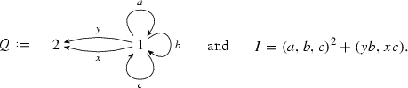
  This is not ideally ordered since there are no surjections between Rb and Rc, however still has good left approximations. It is a short exercise to find the five isomorphism classes of indecomposable principal ideals and calculate their minimal left approximations. All but one of these minimal approximations are surjective, and the one which is not surjective has cokernel $S_1$, the simple at vertex 1. There are no morphisms from $S_1$ to any principal ideal, and hence has good left approximations.

• (b) Let $n>0$ be an integer. Consider the non-monomial algebras $R_n=kQ/I_n$ where

  

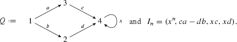
  Again, has good left approximations; it is a short exercise to find the $n+3$ principal ideals and calculate that the minimal left approximation for each one is surjective.

Proposition 2.9

The algebra is left strongly quasi-hereditary with respect to the ideal layer function l if and only if has good left approximations with respect to l.

Proof

Assume has good left approximations . Using the condition on and applying yields a short exact sequence

$$\begin{aligned} 0 \rightarrow P(\Gamma _{>\gamma }) \xrightarrow {\iota (\Gamma )\,} P(\Gamma ) \rightarrow \Delta (\Gamma ) \rightarrow 0, \end{aligned}$$

(3)

where and $\Delta (\Gamma )$ denotes the cokernel of $\iota (\Gamma )$. We claim that the ideal layer function defines a left strongly quasi-hereditary structure on such that the $\Delta (\Gamma )$ are standard modules. To see this we have to show that (3) satisfies conditions (a) and (b) outlined in Definition 2.3. Since all direct summands of $P(\Gamma _{>\gamma })$ are of the form $P(\Lambda )$ with $l(\Lambda ) > \gamma$ condition (a) is satisfied by construction. Using the anti-equivalence - condition (b) translates to: every R-linear non-isomorphism $\nu :\Gamma \rightarrow \Lambda$ with factors over . By definition of this holds for . If , then $\nu$ cannot be surjective for otherwise it is an isomorphism since . Therefore, $\mathsf {im}\,\nu \subsetneq \Lambda$ is a principal left R-ideal with $l(\mathsf {im}\,\nu ) > l(\Lambda )=\gamma$. So $\nu$ factors over .

To see the converse direction, assume does not have good left approximations. Then there exists a principal left R-ideal $\Gamma$ such that . Assume that is quasi-hereditary with respect to the ideal layer function l and let $\Delta (\Gamma )$ be the standard module corresponding to $\Gamma$. Since is a minimal left approximation

is the start of a minimal projective resolution of $\Delta (\Gamma )$. By our choice of $\Gamma$ the morphism is not injective. Hence $\Delta (\Gamma )$ has projective dimension greater than 1 and, using Definition 2.2, A is not left strongly quasi-hereditary with respect to l in this case.$\square$

Remark 2.10

Assume that is quasi-hereditary with respect to the ideal layer function. One can show that as a set the standard module $\Delta (\Gamma )$ is given by all (residue classes of) monomorphisms starting in $\Gamma$. Indeed if $\nu :\Gamma \rightarrow \Lambda$ is not a monomorphism then an argument along the lines of the proof of the proposition shows that $\nu$ factors over and therefore corresponds to the zero element in $\Delta (\Gamma )$.

Proposition 2.9 is related to [35, Theorem 5] by Ringel. He shows that for an R-module M there exists an R-module N such that is left strongly quasi-hereditary and all the indecomposable summands N are submodules of M. In particular, if M is an R-module such that all submodules are isomorphic to direct summands of M, then $\text {End}_R(M)$ is left strongly quasi-hereditary. We will see in Theorem 5.1 that has this property if R is ideally ordered monomial. However, our proof of Theorem 5.1 uses Proposition 2.9, so we cannot apply Ringel’s result in our approach.

Now we look at the ‘dual’ side. First we ‘dualise’ Definition 2.6 using the same notation.

Definition 2.11

For every principal left ideal $\Gamma$ there is a minimal right approximation with . We say that has good right approximations if

Since contains R as a direct summand this is equivalent to for all principal left R-ideals $\Gamma$.

Example 2.12

• (a) Let R be a finite dimensional monomial algebra. Then has good right approximations. Indeed, let $\Gamma$ be a principal left R ideal. Since R is monomial, $\mathsf {rad}\,\Gamma$ is a direct sum of principal left ideals in and the natural inclusion $\mathsf {rad}\,\Gamma \rightarrow \Gamma$ gives the desired minimal right approximation .

• (b) The algebra in Example 2.8 (b) does not have good right approximations: the minimal right approximation of the projective module $P_1$ is and this has kernel $S_4$.

The following result is proved dually to Proposition 2.9

Proposition 2.13

is right strongly quasi-hereditary with respect to the ideal layer function l if and only if has good right approximations. For example, this holds if R is finite dimensional monomial.

Combining Propositions 2.9 and 2.13 with Lemma 2.7 and Example 2.12 (a) yields the following theorem.

Theorem 2.14

If R is an ideally ordered monomial algebra, then is both left and right strongly quasi-hereditary with respect to the ordering induced by the ideal layer function.

We let and denote the full subcategories of -$\text {mod}$ of objects filtered by standard and costandard modules respectively.

Remark 2.15

Assume that is quasi-hereditary with respect to the ideal layer function. Similarly to the case above, one can show that as a set a costandard module $\nabla (\Lambda )$ is given by all surjections ending in $\Lambda$. In particular, each costandard module has head $S(\Pi )$ for some indecomposable projective R-module $\Pi$ and .

Corollary 2.16

If has good right and left approximations, then is closed under submodules and is closed under quotients.

Proof

If has good left approximations, then is left strongly quasi-hereditary by Proposition 2.9, and hence all standard objects have projective dimension 1. By [35, Proposition A.1], all standard modules having projective dimension 1 is equivalent to being closed under quotients.

The analogous dual statement, using Proposition 2.13, shows that when has good right approximations then is closed under submodules.$\square$

3 The characteristic tilting module and Ringel duality

In the following section we first recall the characteristic tilting module T associated to a quasi-hereditary algebra. Then we show that our algebras are ultra strongly quasi-hereditary in the sense of Conde [12] and use this to determine a subcategory of the additive hull of T (Corollary 3.6). In the proof of our main Theorem 5.1 we show that these categories coincide for ideally ordered monomial algebras R and as a consequence establish our Ringel duality formula in this setup.

The following proposition can be found in Ringel [34], which is based on work of Auslander and Reiten [3] and Auslander and Buchweitz [2].

Proposition 3.1

Let A be a quasi-hereditary algebra. Then there exists a tilting module $T \in A$-$\mathrm{mod}$ such that

where is the full subcategory of A-modules with filtrations by both standard and costandard modules.

Definition 3.2

A tilting module T occurring in Proposition 3.1 is called a characteristic tilting module. The Ringel dual $\mathfrak {R}(A)$ of an algebra A is defined by

for T the basic characteristic tilting module consisting of one copy of each indecomposable module in up to isomorphism: i.e. we assume $\mathfrak {R}(A)$ is a basic algebra.

The notion of an ultra strongly quasi-hereditary algebras was introduced by Conde, see [12, Section 2.2.2].

Definition 3.3

A quasi-hereditary algebra A is left ultra strongly quasi-hereditary if a projective module $P_i$ is filtered by costandard modules whenever the corresponding costandard module $\nabla _i$ is simple.

Let be the idempotent corresponding to the direct summand R of . Note that $e_0$ is primitive if and only if R is local. We have the following.

Proposition 3.4

Let R be a finite dimensional algebra. Assume that has good left approximations, so that is left strongly quasi-hereditary with respect to the ideal layer function l. Then the following conditions are equivalent:

• (a) is filtered by costandard objects.

• (b) $\alpha _{\Gamma }:\Gamma \rightarrow \Gamma _{>\gamma }$ is surjective for all principal R-ideals $\Gamma$.

• (c) is left ultra strongly quasi-hereditary.

If R is monomial then these conditions are equivalent to

• (d) R is ideally ordered.

Proof

We first show that (b) implies (a). By [34, Theorem 4], it suffices to show that for all principal left R ideals $\Gamma$ and all primitive idempotents $e_i \in R$. We can assume that $\Delta (\Gamma )$ is not projective. Then applying to produces the projective resolution

$$\begin{aligned} 0 \rightarrow P(\Gamma _{>\gamma }) \xrightarrow {\iota (\Gamma )\,} P(\Gamma ) \rightarrow \Delta (\Gamma ) \rightarrow 0, \end{aligned}$$

and we have to show that every morphism $P(\Gamma _{>\gamma }) \rightarrow P(Re_i)$ factors over $\iota (\Gamma )$. Applying the anti-equivalence given in equation (2) translates this statement to: every morphism $\varphi :Re_i \rightarrow \Gamma _{>\gamma }$ factors over . This holds since $Re_i$ is projective and is surjective by assumption.

Conversely, if is not surjective for some principal ideal $\Gamma$ then there exists . Since R is free there is an R-linear map $R \rightarrow \Gamma _{>\gamma }$, $1 \mapsto x$, which by construction does not factor over . In combination with the anti-equivalence and projective resolution above this shows and [34, Theorem 4] completes the proof that (a) implies (b).

That (a) is equivalent to (c) follows from the fact that $\nabla (\Lambda )$ is simple if and only if $\Lambda$ is projective, see Remark 2.15, and hence $\nabla (\Lambda )$ simple implies $P(\Lambda )$ is a direct summand of .

Let R be monomial. The implication (d) $\Rightarrow$ (b) follows from Lemma 2.7. We now assume (b) and prove the converse.

Firstly, for any indecomposable principal ideal $\Gamma$ the minimal left approximation is surjective by assumption (b), and we claim that $\Gamma _{>\gamma }$ is indecomposable.

To show this take $p \in eR$ for e a primitive idempotent and consider the principal ideal $\Gamma \cong Rp$. Now suppose that there is a decomposition for some principal ideals $Rq_i$. As $\alpha _{\Gamma }$ is surjective, after relabelling we can assume that the image of p is and $q_1 \ne 0$. As the morphism is surjective there must exist some $r \in Re$ such that ; i.e. $rq_1 =q_1$ and for $j \geqslant 2$. As R is monomial, by considering the monomial of lowest degree occurring in $q_1$ and $rq_1 =q_1$ we can see that the degree 0 primitive idempotent e must occur in r. Then we can rewrite $r=e+r'$ where all monomials occurring in $r'$ have degree greater than 0. As a result, must be zero as so there can be no non-zero monomial of lowest degree occurring in . Hence for $j\geqslant 2$, the decomposition is a trivial decomposition , and $\Gamma _{> \gamma }$ is indecomposable.

This allows the successive construction of left $\mathsf {pi}_{>k}$ approximations starting with the indecomposable principal ideal Re

$$\begin{aligned} Re \xrightarrow {\alpha _{Re}\,} Re_{>i_1} \xrightarrow {\alpha _{{Re}_{>i_1}}} Re_{>i_2} \xrightarrow {\alpha _{Re_{>i_2}}} \cdots \xrightarrow {\alpha _{Re_{>i_{n-1}}}} Re_{>i_n} \end{aligned}$$

where $i_1=l(Re)$, , and is the minimal left approximation. Each is indecomposable, and the composition $\alpha _k:Re \rightarrow Re_{>i_k}$ of the left approximations is again a left approximation.

We claim that any indecomposable principal ideal Rx with $x \in eR$ is isomorphic to one of these successive approximations. To see this choose k to be maximal such that $l(Rx) > i_k$. Then there is a surjection $\pi :Re \rightarrow Rx$, and as this must factor through the left approximation $\alpha _k:Re \rightarrow Re_{>i_k}$ by a surjection $\phi :Re_{>i_k}\! \rightarrow Rx$. In particular, $\dim Re_{>i_k} \!\geqslant \dim Rx$ so $l(Re_{>i_k}) \leqslant l(Rx)$. But, by the definition of k, it is true that , hence it must be the case that $l(Re_{>i_k}) = l(Rx)$ so $\dim Re_{>i_k} \!=\dim Rx$ and hence the surjective morphism $\phi$ is an isomorphism $Re_{>i_k} \! \cong Rx$.

Finally, any pair Rx and Ry of principal ideals with $x, y \in eR$ occur (up to isomorphism) in the successive approximation sequence, in which every morphism is surjective by assumption (b), and hence there is a surjection between them. This proves that the ideally ordered condition holds.$\square$

Example 3.5

The non-monomial algebra in Example 2.8 (b) satisfies the equivalent conditions (a), (b) and (c) of the theorem.

Corollary 3.6

Suppose that has both good left and right approximations. Then .

Proof

By the definition of a quasi-hereditary algebra every projective module is filtered by standard modules. Therefore, and by Proposition 3.4 (a), we also have . Now Corollary 2.16 yields and . This implies the claim.$\square$

Remark 3.7

In combination with Remark 2.15, we see that when has both good left and right approximations . For ideally ordered monomial algebras R, Theorem 5.1 (e) shows that holds as well.

Remark 3.8

Let $R=R_2$ be the non-monomial algebra from Example 2.8 (b). The algebra is left ultra strongly quasi-hereditary with respect to the ideal layer function (in particular, is filtered by costandard modules) but not right strongly quasi-hereditary, so is not closed under subobjects. It turns out that there is precisely one indecomposable subobject of which is not filtered by standard modules. This module is also a quotient of and therefore . Restricting to the local submodules of yields the desired inclusion into in this case and can be used to show a version of the Ringel duality formula (10) in this example. Unfortunately, we do not know how to fit this example into a larger framework.

4 An equivalence from idempotents

In this section, we show that there is an equivalence of categories

where for a finite dimensional algebra R with finitely generated and $e_0 \in A$ is the idempotent corresponding to the projection onto R.

To show this we recall several well-known lemmas.

Lemma 4.1

Let be an abelian category with Serre subcategory and let be the quotient functor. Then the restriction of q,

is fully faithful. Here

Proof

This follows from the description of homomorphism spaces in the quotient category as colimits. Indeed for the colimit describing is taken over the single pair of subobjects (X, 0) and the quotient functor sends a morphism $f:X \rightarrow Y$ to f.$\square$

The following lemma can be found in [21, Proposition 5.3 (b)]

Lemma 4.2

Let B be a noetherian ring and let $e \in B$ be an idempotent. Then

$$\begin{aligned} F={\mathrm{Hom}}_B(Be, -):B\text {-}\mathrm{mod}\rightarrow eBe\text {-}\mathrm{mod}\end{aligned}$$

is an exact quotient functor with kernel $B/BeB\text {-}\mathrm{mod}$. In particular, $B/BeB\text {-}\mathrm{mod}$ is a Serre-subcategory in $B\text {-}\mathrm{mod}$.

Corollary 4.3

In the notation of Lemma 4.2, we have .

Proof

Consider and $M \in B/BeB$-$\mathrm{mod}$. Applying the right exact functor ${\mathrm{Hom}}_B(-,M)$ to the surjection $Be \rightarrow N \rightarrow 0$ yields the injection $0 \rightarrow {\mathrm{Hom}}_B(N,M) \rightarrow {\mathrm{Hom}}_B(Be,M)$. As B / BeB-$\mathrm{mod}$ is the kernel of ${\mathrm{Hom}}_B(Be,-)$ and $M \in B/BeB$-$\mathrm{mod}$ it follows that ${\mathrm{Hom}}_B(Be,M)=0$ and hence ${\mathrm{Hom}}_B(N,M)=0$.$\square$

From now on let for some finite dimensional algebra R, such that is finitely generated.

Lemma 4.4

In the notation of Sect. 3, we have $\mathsf {soc} \, Ae_0 \subseteq S_0^{\oplus n}$ for some natural number n. Here is the semi-simple head of $Ae_0$.

Proof

Indeed $Ae_0$ consists of all R-homomorphisms . Let $\Lambda$ be a principal left R-ideal. If $R \rightarrow \Lambda$ is non-zero, then the composition with the canonical inclusion $R \rightarrow \Lambda \rightarrow R$ is non-zero. Therefore every maximal sequence of non-zero morphisms starting in R ends in R, proving the claim.$\square$

Corollary 4.5

.

Proof

Assume that $f :X \rightarrow U$ is a non-zero map, where U in and X in $A/Ae_0A \text {-} \mathrm{mod}$. Lemma 4.4 implies that $\mathsf {im}\,f$ contains a non-zero direct summand of $S_0$. But $\mathsf {im}\,f \in A/Ae_0A \text {-} \mathrm{mod}$ since X is contained in $A/Ae_0A\text {-} \mathrm{mod}$. It follows that $\mathsf {im}\,f$ has no submodule which is a direct summand of $S_0$. A contradiction. So there is no non-zero morphism $f:X \rightarrow U$.$\square$

The following statement is the main result of this section.

Proposition 4.6

The exact functor $F={\mathrm{Hom}}_A(Ae_0, -)$ restricts to an additive equivalence

Proof

The equality on the right follows from the fact that . Since F is exact and maps an A-module M to $e_0M$, the restriction is well-defined. We can apply Lemma 4.1 to $q=F$ to deduce that F is fully faithful. Indeed, by Lemma 4.2, F is a quotient functor corresponding to the Serre subcategory $A/Ae_0A\text {-}\mathrm{mod}$ and Corollaries 4.3 and 4.5 show that the required orthogonality conditions are satisfied.

It remains to show that F is essentially surjective. Let $U \subseteq (e_0Ae_0)^{\oplus n}$ be generated by $u_1, \ldots , u_n \in (e_0Ae_0)^n$. The $u_i$ are elements of $(Ae_0)^n$. Let $V \subseteq (Ae_0)^{\oplus n}$ be the A-submodule generated by the $u_i$. One can check that $F(V)=U$ and since $e_0 u_i=u_i$ for all i V is a factor module of $(Ae_0)^{\oplus m}$ for some m. This shows that V is contained in and completes the proof. $\square$

5 Proof of Ringel duality formula

In this section we prove the following main result of this paper, which is an extended version of Theorem 1.2 stated in the introduction.

Theorem 5.1

Let R be a finite dimensional ideally ordered monomial algebra and . Then is quasi-hereditary and the Ringel duality formula

holds. More explicitly, where $\dagger$ denotes the standard k-duality,

(4)

and if we consider and as exact categories with split exact structures then this Ringel duality induces the derived equivalence

Moreover:

• (a) Every indecomposable submodule of $R^n$ is isomorphic to a principal left ideal, every principal left ideal is isomorphic to a monomial ideal, and hence so .

• (b) The algebra is left and right strongly quasi-hereditary with respect to the ideal layer function. In particular, has global dimension at most 2. Moreover, it is left ultra strongly quasi-hereditary in the sense of Conde [12].

• (c) The ideal order is the unique order defining a quasi-hereditary structure on if R is local and satisfies the following condition: if there exists a surjection $\Lambda \rightarrow \Gamma$ between principal left ideals, then there is an inclusion $\Gamma \rightarrow \Lambda$.

• (d) Let T be the characteristic tilting module of and be the idempotent corresponding to R. Then there is an equality of subcategories . In other words, the indecomposable direct summands $T_i$ of T are precisely those indecomposable -modules which are both quotients and submodules of the projective module .

• (e) We can describe the subcategories and of -$\mathrm{mod}$ as follows:

  

  (5)
  

  (6)

Proof

We first prove the main Ringel duality formula, and in the process also prove (a) and (d). Let and let be the idempotent corresponding to R. By Corollary 3.6, we have an inclusion

(7)

where T is the characteristic tilting module for . In combination with Proposition 4.6, we get an inclusion

(8)

since . Let p (respectively, $p^{\mathrm{op}}$) be the number of indecomposable direct summands of (respectively, ) By definition of , the number p also equals the number of simple -modules. Which in turn equals the number of indecomposable summands of T since T is tilting. Let s (respectively, $s^{\mathrm{op}}$) be the number of indecomposable direct summands of (respectively, ). By (8), $s^{\mathrm{op}} \leqslant p$ (in particular, $s^{\mathrm{op}}$ is finite). Moreover, implies $p \leqslant s$. It follows from [36, Theorem 1.1] that $s=s^{\mathrm{op}}$. Summing up, we have that . In particular, this yields equivalences , and therefore so proves (a). Moreover, using and Proposition 4.6 the inclusions (7) and (8) are equivalences

(9)

In particular, this shows part (d).

By definition, the Ringel dual of is . Using we obtain . Under the standard k-duality the latter identifies with . This completes the proof of the main Ringel duality statement as given in formula (4). As a consequence we get the equivalence .

We now consider part (b). By part (a) we know , and as R is ideally ordered Theorem 2.14 implies that is both left and right strongly quasi-hereditary with respect to the ideal layer function. An algebra which is left and right strongly quasi-hereditary with respect to the same ideal layer function has global dimension at most two by [35, first Proposition in A.2]. Proposition 3.4 shows that is also left ultra strongly quasi-hereditary, and so completes the proof of statement (b).

We now prove (c). Let denote the number of simple -modules S that occur in a Jordan Hölder filtration of an -module M. If a partial ordering on I induces a quasi-hereditary structure, then $[\Delta _i,S_i]=1$ for all $i \in I$; as k is algebraically closed this is equivalent to , see [18, Lemma 1.6].

Using the additional assumption in (c) that R is local, the ideally ordered condition produces a surjection between any two summands of (as all principal ideals are monomial by Lemma 7.3). Hence the ideal layer function induces an ordering on the summands of of the form $\Lambda _0< \Lambda _1< \cdots < \Lambda _t$. Now consider another partial order that also produces a quasi-hereditary ordering.

We first prove that both orderings have the same maximal element. If $\Lambda _i$ is maximal with respect to the new order, then the projective module is also a standard module in this order. If the new order gives rise to a quasi-hereditary structure then, as $P_i$ is standard in this ordering, . As $P_i$ is projective . Under the anti-equivalence , described in formula (2), this implies $\dim \text {End}_{R}(\Lambda _i) =1$. Hence the identity morphism must equal socle projection so $\Lambda _i$ is the simple R-module, which is unique as R is assumed to be local. The simple R-module is the largest summand $\Lambda _t$ of under the ideal layer function ordering, and hence $i=t$.

Secondly, we assume that the orderings match for $k, k+1, \dots , t$, let be an immediate predecessor of $\Lambda _k$ under the new order, and aim to show that $j=k-1$. As R is ideally ordered there is a surjection between and (where exists as $j<k\leqslant t$). As they are labelled by the ideal layer function and there is a surjection . By the condition assumed in (c), the existence of this surjection implies an inclusion . Together these produce a non-trivial endomorphism which does not factor over $\Lambda _i$ for $i>j+1$. Using the anti equivalence again, this translates into a non-trivial endomorphism of that does not factor over $P_i$ for $i>j+1$. In particular, the standard object under the new order is the cokernel of a morphism where the summands of P are projective modules $P_i$ such that $i>j$ under the new ordering, see [18, Lemma 1.1$'$]. If $k \ne j+1$, then both the trivial endomorphism and the non-trivial endomorphism constructed above do not factor via P and hence . By considering the images of these morphisms we see . This would imply that the new ordering does not give a quasi-hereditary structure. Therefore $j=k-1$.

Finally, by proceeding in this way we recover the ideal order and conclude that there is only one quasi-hereditary structure.

We show part (e). To prove (5), we explain the following chain of subcategories

By part (b), is right strongly quasi-hereditary. The first equality holds for all right strongly quasi-hereditary algebras, for example by a dual version of [35, Proposition A.1]. Using (9) and part (a), we see that so . The next inclusion follows from . The last inclusion holds for any right strongly quasi-hereditary algebra using that , which is closed under submodules as noted in Corollary 2.16. Using (9) and the fact that is left ultra strongly quasi-hereditary by part (b), dual arguments establish the following chain

(the last inclusion was also shown in the proof of Corollary 3.6). This implies (6) and completes the proof of part (e). $\square$

For a monomial algebra R there is an equivalence of additive categories , and so is Morita equivalent to

This construction is considered in the general context of pre-radicals in Conde’s thesis. An additional special feature of the ideally ordered algebras is that , and this property does not hold for general monomial algebras. For example, consider the following example that was communicated to us by Xiao-Wu Chen.

Example 5.2

Let R be the path algebra of the following quiver with monomial relations.

Then the left ideal is indecomposable but not principal.

Remark 5.3

We give several further remarks on this result.

(1) For the non-monomial algebra $R=R_2$ in Example 2.8 (b), formula (4) from the theorem fails but the following Ringel duality formula holds:

(10)

For ideally ordered monomial algebras this formula coincides with formula (4) above. Unfortunately, we were not able to find a more general setup where the formula (10) works.

Knörrer invariant algebras [27, Section 6.4.], see Example 1.4 (3) and Sect. 6.1, and truncated free algebras satisfy the additional condition imposed in (c).

(2) The statement that is related to Ringel’s [36, Remark before Corollary 2.2]. It would be interesting to see in what generality this equivalence holds.

We observe that it holds for where p runs over all paths of length 3, which is not ideally ordered but in which every principal left ideal is isomorphic to a monomial ideal. Indeed, in this case the equivalence is given by a tilting module which is obtained by mutating the characteristic tilting module (for the quasi-hereditary algebra structure defined by the ideal layer function) once.

(3) Consider , which is an ideally ordered finite dimensional local monomial algebra. Then there is a surjection $Rx \rightarrow Ry$ but Ry does not include into Rx. One can check that the order $R< Ry< Rx < Rx^2$ on indecomposable submodules of R defines a (left but not right strongly) quasi-hereditary structure on . In particular, in this case the ideal order is not the unique quasi-hereditary order.

(4) Part (c) can fail if R is not local (even if all the other conditions are satisfied). Indeed consider for example the algebra $R=kQ/J^2$ where

and J is the ideal generated by all arrows. Then R is ideally ordered and for every surjection between principal left ideals $\Gamma \rightarrow \Lambda$ there is an inclusion $\Lambda \rightarrow \Gamma$. The order $P_2< P_1 < S_1$ defines a quasi-hereditary structure on which is not left strongly quasi-hereditary. Hence, it differs from the quasi-hereditary structure defined by the ideal layer function (where $P_2=P_1<S_1$), and there is no unique quasi-hereditary structure in this case.

(5) It is true that R is ideally ordered iff $R^{\mathrm{op}}$ is ideally ordered, and using this fact one can also prove the theorem without relying on Ringel’s result [36, Theorem 1.1].

6 Applications and examples

We discuss some relationships between Theorem 5.1 and several classes of algebras that have been studied in separate work.

6.1 Hille and Ploog’s algebras

The results of this paper were originally motivated by an investigation in [27] of a class of geometrically inspired quasi-hereditary algebras introduced by Hille and Ploog [24] for which the Ringel duality formula has a geometric interpretation, and we briefly recall this geometric setup and these algebras below.

As the geometric background, consider a type $A_n$ configuration of intersecting rational curves $C_1, \dots , C_n$ in a smooth, rational, projective surface X with negative self-intersection numbers . Starting with this data, Hille and Ploog consider the full triangulated subcategory

where we recall that denotes the line bundle occurring as the ideal sheaf of an effective divisor $D \subset X$. Hille and Ploog show that this subcategory carries an (exact) tilting object $\Lambda$. To do this they make use of universal (co)extensions, see [18] and also [23] for the special case of vector bundles on a rational surface. We briefly recall the definition in this setting.

Definition 6.1

Consider an ordered pair of vector bundles on a smooth projective rational surface X. Their universal (co)extension is defined to be the vector bundle occurring in the middle of the short exact sequence

where both sequences are determined by the identity element in .

Hille and Ploog show that

is an exceptional sequence of line bundles and that iterated universal extension along this sequence produces a tilting bundle $\Lambda$, see [24, Section 2]. This defines a corresponding algebra

where we assume that $\Lambda$ is taken to be a basic representative of the tilting object. These algebras are quasi-hereditary by construction.

We note that the algebra depends on the choice of consecutive ordering for the labelling of the curves and that there are two choices, $C_1, \dots , C_n$ or $C_n, \dots , C_1$, for the same geometric set up that produce two different algebras and . This phenomenon is explained by the following result.

Proposition 6.2

There is an isomorphism of algebras .

Remark 6.3

The algebra can in fact be realised in the form $E_{R}$ where R is an ideally ordered monomial Knörrer invariant algebra, as we describe below. Then Proposition 6.2 is an consequence of Theorem 5.1. However, the following alternative, short, geometric proof was explained to us by Agnieszka Bodzenta; indeed it was the existence of a Ringel duality formula in this special case that inspired the representation-theoretic generalisation in this paper. Work of Bodzenta and Bondal also realises a Ringel duality associated to birational morphisms of smooth surfaces by gluing t-structures with reversed orderings, see [7].

Proof

Let X be a smooth, rational, projective surface containing a type $A_n$ configuration of rational curves with self-intersection numbers . Consider the exceptional sequence $\mathbb {E}$ in the Hom-finite abelian category . By definition, , where is obtained from $\mathbb {E}$ by taking iterated universal extensions and by passing to a basic representative, see [27, Section 2.3]. On the other hand, taking iterated universal coextensions of $\mathbb {E}$ yields (again we replace this by a basic version if necessary) and it follows from [18, paragraph above Proposition 3.1.] that there is an algebra isomorphism

(11)

where denotes the Ringel dual of $\text {End}_X(\Lambda )$. More precisely, since $\mathbb {E}$ is standardisable, Dlab and Ringel [18, Theorem 2] show that

defines an exact equivalence sending $\mathbb {E}$ to the sequence of standard modules $\Delta _{\Lambda _{\varvec{\alpha }}}$. By Ringel [34, p. 217 and Proposition 2], the characteristic tilting module $T_{\Lambda _{\varvec{\alpha }}} \!\in \mathrm{mod}\text {-}\Lambda _{\varvec{\alpha }}$ is obtained from $\Delta _{\Lambda _{\varvec{\alpha }}}$ by iterated universal coextensions (and passing to a basic module if necessary). In particular, the exact equivalence ${\mathrm{Hom}}_X(\Lambda , -)$ sends T to $T_{\Lambda _{\varvec{\alpha }}}$. Combining this with definition of the Ringel dual we see

as claimed.

Now consider the duality

Then and $T^{\ddagger }$ is obtained from this sequence by iterated universal extensions. By definition, . Since $\ddagger$ is a duality, . In combination with (11) this completes the proof.$\square$

Remark 6.4

We note that there is a change in conventions for compositions of morphisms between this paper and [27]. This corresponds to exchanging algebras with their opposite algebras, or left modules with right modules. The effect this has on the quasi-hereditary structure and Ringel duality is as follows: if A is a quasi-hereditary algebra with defining layer function L and characteristic tilting module T, then $T^{\dagger }$ is the characteristic tilting module for $A^\mathrm{op}$ where $\dagger :A\text {-}\mathrm{mod}\rightarrow A^{\mathrm{op}}\text {-}\mathrm{mod}$ denotes the standard k-duality and the layer function on $A^{\mathrm{op}}$ on is $L^{\dagger }$ defined by . In particular, $\mathfrak {R}(A^{\mathrm{op}}) \cong \mathfrak {R}(A)^{\mathrm{op}}$.

We briefly recap how the algebras $\Lambda$ defined by Hille and Ploog fit into the general setup of Theorem 5.1. To do so we recall the definition of the Hirzebruch–Jung continued fraction expansion, the Knörrer invariant algebras $K_{r,a}$, and a description of the form $\Lambda _{\varvec{\alpha }} \cong E_{K_{r,a}}$.

Definition 6.5

For coprime integers $0<a<r$ the Hirzebruch–Jung continued fraction is the collection of integers $\alpha _i \geqslant 2$ defined by

Definition 6.6

([27, Definitions 4.6, 6.20 and Corollary 6.27]) For coprime integers $0<a<r$ the Knörrer invariant algebra $K_{r,a}$ is defined to be

where the parameters $l \geqslant 1$ and $\beta _i \geqslant 2$ are defined by the Hirzebruch–Jung continued fraction expansion for the fraction $r/(r-a)$.

We recall that the results of [27, Section 6.4] describe the monomial ideal structure on $K_{r,a}$, and in particular combining [27, Theorem 6.26] and [27, Propositions 6.22 and 6.24] yields the following result.

Proposition 6.7

The Knörrer invariant algebra $K_{r,a}$ is an ideally order monomial algebra and there is an isomorphism of quasi-hereditary algebras where is defined by the Hirzebruch–Jung continued fraction expansion of r / a.

Suppose that  mod r. If , then . Similarly, if , then . Using this result it can be seen from the explicit definition of $K_{r,a}$ that . As a result by Proposition 6.7, and hence Theorem 5.1 is a generalisation of Proposition 6.2.

6.2 Example of an application of the Ringel duality formula

In this section we consider as an example the pair of algebras $\Lambda _{[3,2]}$ and $\Lambda _{[2,3]}$. After giving explicit presentations, we discuss their relationship via Ringel duality, their construction from related Knörrer invariant algebras, and explicitly list the distinguished modules in their quasi-hereditary structures in order to verify the Ringel duality formula.

Firstly, by [27, Proposition 6.18] the algebras $\Lambda _{[3,2]}$ and $\Lambda _{[2,3]}$ can respectively be presented as the path algebra of the following quivers with relations:

and

Secondly, the Ringel duality formula of Proposition 6.2 states that

Thirdly, by Proposition 6.7 the corresponding Knörrer invariant algebras are

and these can be presented via the following monomial diagrams:

where the nodes represent the monomial basis of $K_{r,a}$ with the root of the tree representing 1 and the arrows labelled i representing left multiplication by $z_i$ of the node at the source equalling the node at the target. Using these monomial diagrams one can show that $K_{[3,2]} \cong K_{[2,3]}^{\mathrm{op}}$ and to calculate all the left monomial ideals. The left monomial ideals for $K_{[3,2]}$ are $M_0 \cong (1)$, $M_1 \cong (z_1)$ and $M_2 \cong (z_2 z_1)$ and the left monomial ideals for $K_{[2,3]}$ are $N_0 \cong (1)$, $N_1 \cong (z_1)$ and $N_2 \cong (z_1^2)$. These can represented pictorially as subsets of the monomial diagrams by

It is explicit that and .

In order to explicitly verify the Ringel duality formula in this case we first describe the quasi-hereditary structure by calculating the projective $P_i$, injective $I_i$, standard $\Delta _i$, costandard $\nabla _i$, and characteristic tilting $T_i$ objects for each algebra. We list these modules in the table below in terms of the simples, $S_i$ notated by i, occurring in their composition series with the heads written at the top.

Using these descriptions of the characteristic tilting modules, it is a short exercise to verify the Ringel duality formula by direct calculation:

and

Remark 6.8

We observe some further properties of, and relations between, the modules in the tables above. These are all special cases of the general theory developed above.

(1):

If $i \leqslant j$ in the partial order, then there is an inclusion (and a projection ). This holds for all left (respectively right) strongly quasi-hereditary algebras. In other words, in this situation it is a consequence of Theorem 2.14.

(2):

Every submodule of a standard module $\Delta _i$ or a projective module $P_i$ is filtered by standard modules. This is a consequence of Corollary 2.16. Dually, quotients of costandard modules $\nabla _i$ or injective modules $I_i$ are filtered by costandard modules, again by Corollary 2.16.

(3):

For both algebras the only simple costandard module is $\nabla _0$. One can check that the corresponding projective modules $P_0$ are filtered by costandard modules. This illustrates Proposition 3.4 in these cases.

$(3^\mathrm{op})$ :

For both algebras the only simple standard module is $\Delta _0$. The corresponding injective hulls $I_0$ are not filtered by standard modules. In other words, the algebras $\Lambda _{[3,2]}$ and $\Lambda _{[2,3]}$ are not right ultra strongly quasi-hereditary.

(4):

The summands $T_i$ of the characteristic tilting module are precisely those indecomposable modules which are both quotients and submodules of the projective module $P_0$, see Theorem 5.1 (d). In particular, they have head $S_0$ and a socle in .

6.3 Auslander–Dlab–Ringel algebras

Recent results of Conde–Erdmann [13], and work in Conde’s thesis, produce a Ringel duality formula similar to that of Theorem 5.1 for the class of Auslander–Dlab–Ringel (ADR) algebras.

Definition 6.9

Let R be a finite dimensional algebra of Loewy length $L_R$. Define the additive subcategory

and let be the direct sum of indecomposable elements of the additive category up to isomorphism. Then the associated ADR algebra is defined to be

This is the basic algebra Morita equivalent to . In particular, the indecomposable modules in are exactly those of the form for e a primative idempotent and where is the Loewy length of Re.

Remark 6.10

We remark that the ADR algebra defined here is the opposite algebra of the ADR algebra defined by Conde and Erdmann in [13], however the effect on the quasi-hereditary structure is straightforward as is explained in Remark 6.4.

The ADR algebra is quasi-hereditary for the layer function ; this induces the partial ordering

on indecomposable modules in . Indeed it is left ultra strongly quasi-hereditary (see [11, Section 5]), and Conde and Erdmann obtain the following Ringel duality formula for ADR algebras satisfying a regularity condition; we recall that a module is rigid if its radical and socle series coincide.

Theorem 6.11

Let R be an Artin algebra with Loewy length L. If all projective and injective indecomposable R-modules are rigid with Loewy length L, then

That is, the Ringel dual of is isomorphic to the opposite algebra of .

This formula looks very similar to the formula in Theorem 5.1 of this paper. However, in general and there does not appear to be any reason to think the overlap is large.

For example, ADR algebras are not left and right strongly hereditary in general and so not all ADR algebras are in the algebra class. Moreover, it can be seen that Hille and Ploog’s algebras are not always ADR algebras. Indeed, in the example of Sect. 6.2 the modules are straightforward to calculate from the monomial diagrams, and the additive category generated by such objects can be seen to coincide with the additive category for $R=K_{[3,2]}$ so but not for where .

Indeed, the results of Conde and Erdmann also only describe the Ringel dual of an ADR algebra when the dual is also an ADR algebra. However, as can be seen in the example of Sect. 6.2, there are examples of ADR algebras of the form whose dual is not an ADR algebra but whose Ringel dual can still be described by Theorem 5.1: for $R=K_{[3,2]}$ and

Indeed, it is also straightforward to calculate the socle and radical filtrations in this example and hence clear to see that $K_{[3,2]}$ is rigid whereas $K_{[2,3]}$ is not.

Whilst these classes of algebras may not be related in general, there are cases which fall into both classes of algebras. Recall the monomial algebras of Example 1.4 (2) which are ideally ordered and for which . In particular, in this case is a corner algebra of : i.e. there is an idempotent such that .

Proposition 6.12

Let Q be a finite quiver without sources and J be the two-sided ideal generated by all arrows in Q. Then is an ideally ordered monomial algebra and there is an isomorphism of quasi-hereditary algebras .

Proof

The algebra R has Loewy length m and, as noted in Example 1.4 (2), any monomial ideal is isomorphic to for some $l=1, \dots , m$ and some primitive idempotent $e \in R$, hence R is ideally ordered and . As R is ideally ordered by Theorem 5.1 (a), and hence to show that it is sufficient to show that .

To show this consider an indecomposable object of . This is necessarily of the form for some primitive idempotent $e_i$ corresponding to a vertex $i \in Q$ and integer $l=1, \dots , m$. As Q has no sources it follows that there exists a series of arrows $j_{m-l} \xrightarrow {a_{m-l}\,} \cdots \xrightarrow {a_3\,} j_2 \xrightarrow {a_2\,} j_{1} \xrightarrow {a_1\,} i$ such that the path induces a homomorphism of indecomposable projective R-modules. By construction this has kernel , and hence there is an inclusion . In particular , and hence . Hence .

Whilst the layer functions defining the quasi-hereditary structures on and are not identical in general, we claim that the corresponding orderings do induce the same standard modules and hence the same quasi-hereditary structure on . To show this we let $P_{i,l}$ denote the projective -module and $S_{i,l}$ denote its simple quotient. We recall the order for is defined by and the order for is defined by . In particular, both orderings induce strongly quasi-hereditary structures, and hence for both orderings there are short exact sequences defining the respective standard modules

(12)

for each projective module $P_{i,l}$, see Definition 2.3. Hence to show that the two orderings induce the same quasi-hereditary structure it is sufficient to show that the projective submodules of $P_{i,l}$ appearing in (12) are the same for both orderings. For this we note that under the additive anti-equivalence

an -module is a proper submodule of $P_{i,l}$ if and only if the corresponding R-module is a proper quotient of . This in turn is equivalent to and is also equivalent to $i=j$ and $k<l$. This shows that the two orderings induce the same quasi-hereditary structure.$\square$

It is a natural question whether it is possible to find an expanded class of algebras with a more general Ringel duality formula that encompasses both Theorems 5.1 and 6.11.

6.4 Nilpotent quiver algebras

The nilpotent quiver algebras introduced by Eiriksson and Sauter [20, Section 3] are a class of quasi-hereditary algebras.

Definition 6.13

Let $Q=(Q_0,Q_1)$ be a finite quiver. For $s\in \mathbb {Z}_{>0}$ the nilpotent quiver algebra is defined to be

where $Q^{(s)}$ is the staircase quiver $Q^{(s)}$ defined by having vertices $i_l$ for $i \in Q_0$ and and arrows

and where $J \subset kQ^{(s)}$ is the two-sided ideal generated by the relations

Remark 6.14

We remark again that the nilpotent quiver algebra defined here is the opposite algebra of the nilpotent quiver algebra defined by Eiriksson and Sauter in [20], however the effect on the quasi-hereditary structure is straightforward as is explained in Remark 6.4.

It follows from [20, Proposition 3.15] that all nilpotent quiver algebras $N_s(Q)$ are right strongly quasi-hereditary and left ultra strongly quasi-hereditary for the quasi-hereditary structure determined by the layer function .

In particular, for $R=kQ/J^m$ the ADR and nilpotent quiver algebras are related as follows.

Proposition 6.15

Let Q be a finite quiver, J the two-sided ideal generated by all arrows in Q, and m a positive integer. Then there is an isomorphism of quasi-hereditary algebras

if and only if all projective $kQ/J^m$-modules have Loewy length m: i.e. Q contains no sinks and m is arbitrary or $m=1$ and Q is arbitrary.

Proof

Let $R=kQ/J^m$, and let $e_i \in R$ for $i \in Q_0$ denote the primitive idempotents corresponding to vertices of Q. Up to isomorphism, the indecomposable modules in are exactly for $1 \leqslant l \leqslant L(Re_i)$ and $i \in Q_0$, where $L(Re_i)$ is the Loewy length of the projective $Re_i$.

In particular, the maximal Loewy length of a projective module in is m and so the maximum possible number of non-isomorphic indecomposables in is $m|Q_0|$. But $|Q^{(m)}_0|=m|Q_0|$, so for to be isomorphic to $N_{m}(Q)$ it is necessary that all projective R-modules have Loewy length m.

Now suppose that all projective R-modules do have Loewy length m and consider the algebra . We start by labelling the indecomposable module in corresponding to by $i_l$ and hence label the corresponding primitive idempotent by $e_{i_l}$. There are indecomposable modules $i_{l}$ for $i \in Q_0$ and , matching the definition of the vertices in the staircase quiver $Q^{(m)}$.

We now want to produce a morphism , and to do this we consider the morphisms between the indecomposable modules in . Firstly, there are surjections which we label by arrows for $i \in Q_0$ and .

Secondly, an arrow $a:i \rightarrow j \in Q_1$ corresponds to a morphism of projectives and for each l this induces a morphism with kernel which in turn induces an injective morphism

for each . We label these morphisms by for $a \in Q_1$ and . In particular, the morphisms described here match the arrows of the staircase quiver $Q^{(m)}$ under the identification $a_l=\rho (a)_l$ and . In particular, an arrow $a:i \rightarrow j$ in Q corresponds to a morphism which induces morphisms

where the relations and hold.

This allows us to define a morphism from the path algebra of the staircase algebra $kQ^{(m)}$ to by

and, as the relations imposed on $kQ^{(m)}$ by $N_m(Q)$ are mapped to 0, this induces a morphism

We will now show that $\Phi$ is surjective, and then calculate the dimensions of $N_m(Q)$ and to show that it is an isomorphism.

Suppose that is a morphism

for some $i,j \in Q_0$ and . There is a surjection and so f gives a morphism . There is also a surjection , and as $Re_i$ is projective this induces a uniquely defined morphism such that

As a morphism between projective modules, the morphism corresponds to an element . In particular, $g= \sum _p \lambda _p p \in kQ/J^m=R$ for scalars $\lambda _p$ and homogeneous paths p from j to i in $kQ/J^m=R$ corresponding to morphisms .

We now work with one indecomposable path p, corresponding to a morphism , and suppose that p consists of arrows for $a_i \in Q_1$. We define a corresponding path in $N_m(Q)$ from $i_{l-n}$ to $j_l$ by

for . Similarly, we define the path in $N_m(Q)$

for $i \in Q_0$ and such that $\Phi ( (\pi _{i,l}) ) \cong \pi _{i,l}$. Then the morphism p factors over its kernel, which is , so

Hence

Using the relations in $N_m(Q)$ we can rearrange this expression as

where we note that if g is non-zero then $k-n \leqslant l$ and hence

and hence

Returning to the morphism $g = \sum \lambda _p p$ we see that

and we can now conclude that

where |p| is the length of the path p, but $\pi _{i,l}$ is surjective and hence

We conclude that $\Phi$ is a surjection, and we now show that this surjective morphism is in fact an isomorphism by calculating the dimensions of $N_m(Q)$ and .

We first calculate the dimension of by calculating the dimension of the morphisms between any two indecomposables in . As shown above, a morphism in of the form is induced by a particular element in $kQ/J^m$ corresponding to a morphism of projective modules . Such elements are spanned by the paths, and we now calculate the morphisms in that are induced by such path in $R=kQ/J^m$. These will give a basis for the morphisms . A path $p:j \rightarrow i \in kQ/J^m = R$ of length |p| (under the length grading on Q) induces the morphism which composes to give a non-zero morphism if and only if $|p|<k$. In turn, this descends to give a non-zero morphism if and only if , which occurs if and only if $l \geqslant k-|p|$. As such there are isomorphisms of vector spaces

We then calculate the dimension of $N_m(Q)$ by counting the number of paths between any two vertices. Using the explicit description of $N_m(Q)$ above, any path in $N_m(Q)$ corresponds to the composition of arrows of type $a_l$ and arrows of type , these commute , and . Using these relations any non-zero path can be rearranged such that all the type arrows occur in the path before the $a_l$ type arrows. That is: a path from $i_l$ to $j_k$ in $N_m(Q)$ exactly corresponds to the path in $N_m(Q)$ induced by a path from j to i in Q of length |p| pre-composed with $l-k+|p|$ arrows of type

so that the induced path is from $i_l$ to $j_k$. However, the path is non-zero if and only if the number of type arrows is greater than or equal to 0 and strictly less than l, and it follows that

Hence

It follows that the surjective homomorphism is in fact an isomorphism as . Hence .

Further, under this isomorphism the layer functions defining the quasi-hereditary structures on $N_m(Q)$ and are identified and hence this is an isomorphism of quasi-hereditary algebras.$\square$

Example 6.16

We give a brief example of Proposition 6.15. Consider the quiver

and let J denote the two-sided ideal generated by all arrows. Define , and then we present the two algebras $N_3(Q)$ and .

Firstly, the algebra $N_3(Q)$ is defined to be the path algebra of the quiver with relations

Secondly, we consider the indecomposable modules in . There are six classes and we list them and a basis for all injective or surjective maps between them below.

This describes and matches the path algebra with relations description of $N_3(Q)$ above.

Combining Proposition 6.15 with Proposition 6.12 and Theorem 5.1 (or Theorem 6.11) instantly gives the following corollary.

Corollary 6.17

If Q is a finite quiver without sinks or sources and m is a positive integer, then there are isomorphisms of quasi-hereditary algebras

In particular, the Ringel dual for a nilpotent quiver algebra without sinks or sources is determined by the formula

$$\begin{aligned} \mathfrak {R}(N_m(Q)) \cong N_m(Q^{\mathrm{op}})^{\mathrm{op}}\!. \end{aligned}$$

We note that if Q is a finite quiver with no sinks but with sources then $E_{kQ/J^m}^{\mathsf {ADR}} \cong N_m(Q)$ but (if $m>1$) as $kQ^{\mathrm{op}}$ contains sinks. In particular, Proposition 6.15 and Theorem 6.11 cannot be used to strengthen the Ringel duality formula of Corollary 6.17 to all quivers with no sources.

6.5 Auslander and Nakayama algebras

For a finite dimensional algebra R of finite representation type we define , where the sum is taken over all indecomposable $M \in R\text {-}\mathrm{mod}$ up to isomorphism, and the Auslander algebra is defined to be

Proposition 6.18

If R is an ideally ordered monomial algebra, then if and only if R is self-injective.

Proof

If , hence every injective R-module I embeds into $R^n$. Therefore, I is a direct summand of $R^n$, hence projective, and hence R is self-injective.

Conversely, if R is self-injective, then every injective R-module embeds into $R^n$ for some n and hence every injective module is also a projective module. Then every object in $R\text {-}\mathrm{mod}$ is a submodule of an injective R-module, hence of a projective R-module, hence and .$\square$

The Nakayama algebras, introduced in [31], are a well known class of finite dimensional algebras with finite representation type; see e.g. [4, Theorem VI.2.1]. Recall that a self-injective Nakayama algebra is of the form $kC_n/J^m$ where $C_n$ is an oriented cycle with n vertices and J is the ideal generated by all arrows, see e.g. [1, Theorem 32.4] for the a description of the underlying quiver of a general Nakayama algebra. In particular, the self-injective Nakayama algebras are ideally ordered monomial algebras.

Corollary 6.19

If R is a self-injective Nakayama algebra, then .

It follows from the explicit description $R=kC_n/J^m$ that by Corollary 6.17 and so this corollary recovers the well known explicit description of the Auslander algebras of self-injective Nakayama algebra in terms of quivers with relations. As and $N_m(C_n) \cong N_m(C_n^{\mathrm{op}})^{\mathrm{op}}$ the Ringel duality formula recovers the result of [37] that the Auslander algebras of self-injective Nakayama algebras are Ringel self-dual for the ideal layer function.

Corollary 6.20

For a self-injective Nakayama algebra R, .

Remark 6.21

In order to give another perspective on Proposition 6.18, and Corollaries 6.19 and 6.20, we recall that self-injective finite dimensional monomial algebras R are Nakayama algebras. To see this, we have to show that the quiver Q underlying R is a union of oriented lines and oriented cycles. In other words, at every vertex of Q there is at most one incoming and at most one outgoing arrow. Assume that there is a vertex i with more than one outgoing arrow. Then, as R is monomial, the corresponding indecomposable projective R-module $P_i$ does not have a simple socle - in particular, $P_i$ is not injective contradicting our assumption that R is self-injective. A dual argument shows that Q does not have vertices with more than one incoming arrow.

7 Appendix: Results on finite dimensional monomial algebras

In this section we collect some technical results on finite dimensional monomial algebras $R=kQ/I$ (where I is generated by a collection of paths in Q). We will use the term ‘monomial’ to mean a monomial expression in the generators (i.e. arrows and lazy paths) of such an algebra.

Lemma 7.1

Let R be a monomial algebra and $n, m \in R$ monomials. If there exists a surjection $\phi :Rm \rightarrow Rn$, then the map $Rm \rightarrow Rn$ defined by $m \mapsto n$ is R-linear.

Proof

It suffices to show that $\mathrm {ann}_R(m)$ is contained in $\mathrm {ann}_R(n)$. Take $r \in R$ with $rm=0$, and we aim to show that $rn=0$. We write $r = \sum \lambda _i r_i$ with monomials $r_i$ and non-zero scalars $\lambda _i$. Since R is monomial, it follows that for all i. The existence of a surjection $\phi :Rm \rightarrow Rn$ implies $m, n \in eR$ for some primitive idempotent $e \in R$ and that there exist $s,t \in R$ such that and $\phi (m)=sn$. In particular, $tsn=n$ and so for some non-zero scalars $\mu _i$ and distinct monomials $s_i \ne e$. Therefore , and so as R is monomial it follows that all monomials that make up $r_i s n$ are 0. In particular, $r_i \mu _0 e n=\mu _0 r_i n =0$. This implies that $r_in=0$ for all i, and hence $rn=0$ so $\mathrm {ann}_R(m) \subset \mathrm {ann}_R(n)$ finishing the proof.$\square$

Lemma 7.2

Let $m, n \in R$ be monomials. If R is ideally ordered, then every surjection $Rm \rightarrow Rn$ factors over $\pi :Rm \rightarrow Rn$, $m \mapsto n$.

Proof

Let $\psi :Rm \rightarrow Rn$ be an surjection. In particular, $m, n \in eR$ for some primitive idempotent $e \in R$ and there exist $s,t \in R$ such that $\psi (m)=sn$ and . It follows that $tsn=n$, so $s=\lambda _0 e + \sum \lambda _i s_i \in eRe$ for non-zero scalars $\lambda _i$ and distinct monomials $s_i \ne e$. Hence $sn=\lambda _0 n + \sum \lambda _i s_i n$. In particular, $R s_i n \subsetneq Rn$, and since R is ideally ordered there exists surjections $Rn \rightarrow R s_i n$ which, using Lemma 7.1, we can assume are defined by $n \mapsto s_i n$. Denote the composition of such a surjection with the inclusion $R s_i n \subseteq Rn$ by $\varphi _i$ and define $\varphi :Rn \rightarrow Rn$ as $\varphi = \lambda _0 \mathrm {id} + \sum \lambda _i \varphi _i$. Then $\varphi (n)=sn$ and therefore $\psi = \varphi \pi$ factors as claimed.$\square$

Lemma 7.3

Let $p \in eR$ for a primitive idempotent $e \in R$. If R is ideally ordered, then the principal left ideal Rp is isomorphic to a principal ideal Rm, for a monomial $m \in eR$.

Proof

Since R is monomial, we may write p as linear combination of monomials with $\lambda _i$ non-zero scalars and $p_i \in eR$ monomials. Since R is ideally ordered we may assume that the $p_i$ are labelled in such a way that $Rp_1 \rightarrow Rp_2 \rightarrow \cdots \rightarrow Rp_t$ are surjections.

We now wish to rewrite p so that none of the $p_i$ can be expressed in the form $np_1$ for a monomial n. To do this, let I index the $p_i$ such that there is a monomial $r_{i}$ with $p_{i}=r_{i}p_1$ for $i \in I$. Then we define and . As it follows that $s= \lambda _1 e+r$ is a unit in eRe and there exists $t \in eRe$ such that $st=e$. In particular, $Rtp =Rp$. Then we rewrite for some non-zero scalars and monomials . For each there is some $p_i$ such that by their definition, and hence there are surjections for all j. As $Rtp \cong Rp$ we now work with tp rather than p and tp has the property that there are no with for a monomial n.

We claim that $Rtp \cong Rp_1$, hence $Rp \cong Rp_1$. As there are surjections there are surjections , by Lemma 7.1. Let be the composition of such a surjection with the canonical inclusion and let $\iota :Rp_1 \rightarrow R$ be the canonical inclusion. Define $\psi :Rp_1 \rightarrow R$ by . Then so $\mathsf {im}\,\psi = Rtp$. Hence $\psi$ defines a surjective morphism $\phi :Rp_1 \rightarrow Rtp$.

We must now check that this morphism is also injective. If $\psi (rp_1)=0$, then . As R is monomial if $rp_1$ is non-zero there must exist monomials $n,m \in R$ such that for some j, and if this occurs either or for submonomials $m'$ and $n'$ neither equal e. The first case cannot occur as this implies which contradicts the existence of a surjection . The second situation also cannot occur as the construction of the above ensured none were of this form. Hence $rp_1=0$ so the morphism is also injective and $Rp_1 \cong Rtp \cong Rp$.$\square$

References

Anderson, F.W., Fuller, K.R.: Rings and Categories of Modules. Graduate Texts in Mathematics, vol. 13, 2nd edn. Springer, New York (1992)
Auslander, M., Buchweitz, R.-O.: The homological theory of maximal Cohen–Macaulay approximations. Mém. Soc. Math. France (N.S.) 38, 5–37 (1989)
Auslander, M., Reiten, I.: Applications of contravariantly finite subcategories. Adv. Math. 86(1), 111–152 (1991)
Auslander, M., Reiten, I., Smalø, S.O.: Representation Theory of Artin Algebras. Cambridge Studies in Advanced Mathematics, vol. 36. Cambridge University Press, Cambridge (1997). Corrected reprint of the 1995 original
Auslander, M., Smalø, S.O.: Preprojective modules over Artin algebras. J. Algebra 66(1), 61–122 (1980)
Baur, K., Erdmann, K., Parker, A.: \(\varDelta \)-filtered modules and nilpotent orbits of a parabolic subgroup in \({{\rm O}}_N\). J. Pure Appl. Algebra 215(5), 885–901 (2011)
Bodzenta, A., Bondal, A.: Derived categories of smooth surface contractions (in preparation)
Bodzenta, A., Külshammer, J.: Ringel duality as an instance of Koszul duality (2017). arXiv:1701.06222
Buchweitz, R.-O., Leuschke, G.J., Van den Bergh, M.: On the derived category of Grassmannians in arbitrary characteristic. Compositio Math. 151(7), 1242–1264 (2015)
Cline, E., Parshall, B., Scott, L.: Algebraic stratification in representation categories. J. Algebra 117(2), 504–521 (1988)
Conde, T.: The quasihereditary structure of the Auslander–Dlab–Ringel algebra. J. Algebra 460, 181–202 (2016)
Conde, T.: \(\varDelta \)-filtrations and projective resolutions for the Auslander–Dlab–Ringel algebra. Algebr. Represent. Theory (2017). https://doi.org/10.1007/s10468-017-9730-z
Conde, T., Erdmann, K.: The Ringel dual of the Auslander–Dlab–Ringel algebra (2017). arXiv:1708.05766
Coulembier, K.: Ringel duality and Auslander–Dlab–Ringel algebras (2017). arXiv:1710.08019
Coulembier, K., Mazorchuk, V.: Dualities and derived equivalences for category \({\mathscr {O}}\). Israel J. Math. 219(2), 661–706 (2017)
Crawley-Boevey, W., Sauter, J.: On quiver Grassmannians and orbit closures for representation-finite algebras. Math. Z. 285(1–2), 367–395 (2017)
Dlab, V., Ringel, C.M.: Every semiprimary ring is the endomorphism ring of a projective module over a quasihereditary ring. Proc. Amer. Math. Soc. 107(1), 1–5 (1989)
Dlab, V., Ringel, C.M.: The module theoretical approach to quasi-hereditary algebras. In: Tachikawa, H., Brenner, S. (eds.) Representations of Algebras and Related Topics. London Mathematical Society Lecture Note Series, vol. 168, pp. 200–224. Cambridge University Press, Cambridge (1992)
Erdmann, K., Parker, A.E.: On the global and \(\nabla \)-filtration dimensions of quasi-hereditary algebras. J. Pure Appl. Algebra 194(1–2), 95–111 (2004)
Eiriksson, Ö., Sauter, J.: Quiver-graded Richardson orbits (2017). arXiv:1707.03244
Geigle, W., Lenzing, H.: Perpendicular categories with applications to representations and sheaves. J. Algebra 144(2), 273–343 (1991)
Ginzburg, V., Guay, N., Opdam, E., Rouquier, R.: On the category \({\mathscr {O}}\) for rational Cherednik algebras. Invent. Math. 154(3), 617–651 (2003)
Hille, L., Perling, M.: Tilting bundles on rational surfaces and quasi-hereditary algebras. Ann. Inst. Fourier (Grenoble) 64(2), 625–644 (2014)
Hille, L., Ploog, D.: Tilting chains of negative curves on rational surfaces. Nagoya Math. J. (2017). https://doi.org/10.1017/nmj.2017.40
Iyama, O.: Finiteness of representation dimension. Proc. Amer. Math. Soc. 131(4), 1011–1014 (2003)
Iyama, O., Reiten, I.: 2-Auslander algebras associated with reduced words in Coxeter groups. Int. Math. Res. Not. IMRN 2011(8), 1782–1803 (2011)
Kalck, M., Karmazyn, J.: Noncommutative Knörrer type equivalences via noncommutative resolutions of singularities (2017). arXiv:1707.02836
Krause, H.: Koszul, Ringel and Serre duality for strict polynomial functors. Compositio Math. 149(6), 996–1018 (2013)
Krause, H., Saorín, M.: On minimal approximations of modules. In: Green, E.L., Huisgen-Zimmermann, B. (eds.) Trends in the Representation Theory of Finite-Dimensional Algebras. Contemporary Mathematics, vol. 229, pp. 227–236. American Mathematical Society, Providence (1998)
Kuznetsov, A., Lunts, V.A.: Categorical resolutions of irrational singularities. Int. Math. Res. Not. IMRN 2015(13), 4536–4625 (2015)
Nakayama, T.: Note on uni-serial and generalized uni-serial rings. Proc. Imp. Acad. Tokyo 16, 285–289 (1940)
Nguyen, V.C., Reiten, I., Todorov, G., Zhu, S.: Dominant dimension and tilting modules (2017). arXiv:1706.00475
Pučinskaitė, D.: Quasi-hereditary algebras via generator-cogenerators of local self-injective algebras and transfer of Ringel duality. Math. Z. 279(3–4), 641–668 (2015)
Ringel, C.M.: The category of modules with good filtrations over a quasi-hereditary algebra has almost split sequences. Math. Z. 208(2), 209–223 (1991)
Ringel, C.M.: Iyama’s finiteness theorem via strongly quasi-hereditary algebras. J. Pure Appl. Algebra 214(9), 1687–1692 (2010)
Ringel, C.M.: On the representation dimension of Artin algebras. Bull. Inst. Math. Acad. Sin. (N.S.) 7(1), 33–70 (2012)
Tan, R.: Auslander algebras of self-injective Nakayama algebras. Pure Mathematical Sciences 2(2), 89–108 (2013)
Tsukamoto, M.: Strongly quasi-hereditary algebras and rejective subcategories. Nagoya Math. J. (2018). https://doi.org/10.1017/nmj.2018.9
Acknowledgements
We thank Teresa Conde for interesting discussions about this work and about relations to her thesis. We are grateful to Karin Erdmann for pointing us to Ringel’s paper which simplifies the proof of our main result and adds another perspective to this work. We also thank Agnieszka Bodzenta who, in particular, explained to us the proof of Proposition 6.2 and Xiao-Wu Chen who shared with us Example 5.2. We would also like to thank Ögmunder Eiriksson, Julian Külshammer, Daiva Pučinskaitė, Špela Špenko, and Michael Wemyss for interesting and helpful discussions and David Ploog for pointing out misprints in an earlier version. We would also particularly like to thank the anonymous referee, whose many useful comments have greatly improved the paper.
Author information
Authors and Affiliations
Corresponding author
Additional information
The first author was supported by EPSRC Grant EP/L017962/1. The second author was supported by EPSRC Grant EP/M017516/2.
Rights and permissions
Open Access This article is distributed under the terms of the Creative Commons Attribution 4.0 International License (http://creativecommons.org/licenses/by/4.0/), which permits unrestricted use, distribution, and reproduction in any medium, provided you give appropriate credit to the original author(s) and the source, provide a link to the Creative Commons license, and indicate if changes were made.
About this article
Cite this article
Kalck, M., Karmazyn, J. Ringel duality for certain strongly quasi-hereditary algebras. European Journal of Mathematics 4, 1100–1140 (2018). https://doi.org/10.1007/s40879-018-0250-0
Received:
Revised:
Accepted:
Published:
Issue Date:
DOI: https://doi.org/10.1007/s40879-018-0250-0