
Abstract
Before taking up the ground improvement of a site, assessment of liquefaction potential of a region is very important. This also helps in seismic microzonation of the area. It can be rationally performed if the data of site (using either field tests or laboratory tests) are available. The aim of the present study is to evaluate liquefaction potential of Roorkee (India) region. For this purpose the liquefaction resistance of the soil, within the radius of 30 km of Roorkee, was evaluated using two different approaches. First is the field approach based on standard penetration test (SPT) N-Value and second is the laboratory approach employing mean grain size distribution (D 50). Investigation was carried out at five different locations by conducting SPT tests and collecting soil samples at regular interval. The cyclic shear stress due to earthquake loading was examined using simplified method as well as using ground response analysis. The factor of safety against liquefaction was evaluated at different depths for all the sites using both field and laboratory data. It was found that the factor of safety against the liquefaction using field approach is marginally greater than that using the laboratory approach for all the sites. Also the factor of safety using ground response analysis is significantly smaller than that using simplified method. Thus it was concluded that use of simplified method may not be adequate.
Introduction
One of the most important aspects of ground improvement techniques is the assessment of the need of improvement. During recent major earthquakes, it was observed that the major damage to foundations and structures, was due to liquefaction [1]. Therefore, it is utmost important to determine liquefaction potential of a region before considering any ground improvement.
The phenomenon of liquefaction drawn attention of many researchers after 1964 Alaskan and 1964 Niigata earthquakes. Significant damage to many structures due to liquefaction was observed during earthquakes in last two decades e.g. Kobe, Japan (1995); Chi–Chi, Taiwan (1999); Bhuj, India (2001); and Fukushima, Japan (2011). Many structures traverse over the water bodies, where the soil conditions are loose and saturated. These sites are vulnerable to liquefaction. In 2001 Bhuj earthquake, a large area of the state of Gujarat, India was affected due to liquefaction.
After strong earthquakes, soil liquefaction often had been observed, as one type of ground failure. In many countries, the evaluation of liquefaction potential is considered in seismic code and microzonation. Liquefaction is a very complex phenomenon and has been studied extensively by hundreds of researchers around the world, however, the roadmap is not clear yet. Many researchers reported evaluation of liquefaction potential. Based on grain size, Seed and Idriss [2] proposed the method to determine equivalent uniform average shear stress due to an earthquake. Seed [3] developed a method to estimate liquefaction potential for sand under level ground conditions using standard penetration test (SPT) data. This method was based on field data for the sites, which either had or not experienced liquefaction due to earthquake loading. Seed et al. [4] presented empirical methods for evaluating liquefaction of sands and silty sands by SPT-N value.
For many countries, field data for sites which were known to have a susceptibility to liquefaction during earthquakes were used to establish a criterion for evaluating liquefaction potential of sands in an earthquake of magnitude 7.5. The result of this study was then extended to earthquakes of other magnitudes. A simple procedure for considering the influence of silt content was proposed [4]. The standard penetration test is a widely used method for the evaluation of soil liquefaction potential. Seed et al. [5] developed SPT based method to estimate the liquefaction potential for sands. The field data were reinterpreted and plotted in terms of (N 1)60. i.e. the N value determined by SPT tests in which the driving energy in drill rod is 60 % of the theoretical free fall energy and normalized overburden pressure of 1 ton/ft2 (100 kPa). Liquefaction curves for sands with different (N 1)60 value and different fine contents were proposed [5].
Some researchers [6, 7] developed the SPT based methods for liquefaction analysis. The effect of fines content as well as the effect of nature of fines was presented [6]. Sometime the difference between the results of field and laboratory approaches could be quite large, due to the fact that the specimens tested in the laboratory do not reflect the influence of field factors [8]. Many researchers [9–13] extended previous studies on the use of SPT data for evaluation of liquefaction resistance. Few studies for liquefaction susceptibility of the Solani sand were conducted [14, 15]. The sand is collected from Solani Riverbed near Roorkee. The effects of fines and reinforcement on Solani sand were also presented [16, 17].
Evaluation of liquefaction potential is an important issue for planned development of a city and this helps in the microzonation of the city. Roorkee city is about 200 km North of Delhi and situated in Uttarakhand state of India. Due to industrialization, the city is growing at a very fast rate and it is necessary to identify the seismic hazardous areas. The city lies in seismic zone IV [18] and thus has high seismic risk. Further the soil strata at many places in Roorkee region is Alluviam, therefore, may liquefy during strong earthquake excitation. The liquefaction potential of the Roorkee region is not reported in the literature. The aim of the study is to fulfill this gap by conducting field and laboratory tests.
In the present research work, studies have been carried out for evaluating the liquefaction potential of soil. For this purpose, soil samples from different places of Roorkee region are collected. Field data from five representative boreholes were collected using SPT to know the N values and soil profile for geotechnical investigation. At the end, a comparison of results with similar past studies has been carried out. The results presented in this paper will be helpful for practicing engineers and researchers to identify the areas which have high potential of liquefaction and in turn require ground improvement.
Study Area
The SPT tests were conducted at five different sites in the Roorkee region (within a radius of 30 km). The locations of sites are as follows:
-
(1)
DEQ Campus: open ground of Dept. of Earthquake Engineering, IIT Roorkee.
-
(2)
Solani Riverbed: on the bed of the Solani river (about 50 m from Solani Via aqueduct).
-
(3)
Bhagwanpur: the site is located in the playground of a Govt. Inter College.
-
(4)
Bahadrabad: the site is between Roorkee and Haridwar on NH-58 and drilling was conducted in the ground of Arya Inter College, Bahadrabad.
-
(5)
Haridwar City: the site is in the playground of Bhalla College near the bus stand in city.
From all these five locations, the soil samples were collected through SPT and data collected from field and laboratory tests are analyzed for liquefaction potential. Kirar and Maheshwari [19] evaluated dynamic properties of these soil samples using cyclic triaxial tests.
Details of test sites used in the present study are given in Table 1. Since, the water table rises during the rainy (monsoon) season, therefore for the analysis, the water table is assumed at the ground surface for all the sites.
Methodology
The methodology of analysis includes following three steps;
-
(i)
Evaluating shear stresses due to earthquake (τ av) either by simplified procedure [2] or using ground response analysis [20].
-
(ii)
Evaluating shear stresses causing liquefaction i.e. liquefaction resistance of soil either using simplified procedure based on laboratory tests [2] or based on field tests [5].
-
(iii)
Using information collected in above two steps, factor of safety with depth is computed.
These steps and relevant formulation is described in detail in following subsections.
Shear Stress due to Earthquake Loading (τ av)
The average shear stress due to earthquake loading (τ av) is computed based on the following two methods.
(a) Simplified method [2]:
Cyclic stress ratio (CSR) is defined as
where a max is the peak horizontal acceleration at the ground surface, g is the acceleration due to gravity, σ vo and \(\sigma^{\prime}_{\text{vo}}\) are total stress and effective stress, respectively and r d = stress reduction coefficient, a max depends on the earthquake magnitude and epicentral distance from the rupture zone, for seismic zone IV, a max = 0.24 g is considered [18].
Stress reduction coefficient, describes the flexibility of soil profile. Seed and Idriss [2] presented widely used curve between r d and depth. A new relationship for stress reduction (Eq. 3) is reported by Youd et al. [10] and has been used in the present study
where z is the depth beneath ground surface in meters.
(b) Ground response analysis (GRA): This has been performed using the program EERA [21] which is based on one dimensional layered soil model. The shear wave velocity is an important parameter for the program EERA. The shear wave velocity values with depth at all the five sites were determined from the seismic geophysical field tests: Multi-channel spectral Analysis of Surface Waves (MASW).
The transient excitation (acceleration time history) was used as an input loading to the program EERA. The N79°03′E Component of 2005 Chamoli Earthquake recorded at Chamoli station was used. The acceleration time history [22] of this earthquake is shown in Fig. 1a which indicates PGA equal to 0.06 g. The Fig. 1(b) shows the Fourier spectrum of this earthquake indicating predominant frequencies of 1.5 and 3.0 Hz. The duration of the actual time history is 44.61 s; however, after 30 s, the value of acceleration is negligible, therefore only 30 s duration is considered for analysis. Since the actual PGA for this time history is too low (i.e. 0.06 g) and Roorkee being in seismic zone IV; this acceleration time history is proportionately increased for PGA = 0.2 g and used in the analysis. The maximum shear stresses (τ max) at different depths were computed using the program EERA. The average shear stress (τ av) is computed as (0.65*τ max). The CSR is found as the ratio (0.65*τ max/\(\sigma^{\prime}_{\text{vo}}\)).

a N79°03′E Component of 2005 Chamoli Earthquake Recorded at Chamoli Station b The Fourier spectrum of 2005 Chamoli Earthquake
Shear Stress Required to Cause Liquefaction (τ liq)
Stress causing liquefaction is computed based on two approaches; (a) using laboratory approach i.e. simplified procedure [2] and (b) using field approach based on N values [5].
Shear Stress Based on Laboratory Tests (τ lab)
Evaluation of the cyclic shear stresses causing liquefaction of soil in a given number of stress cycles by means of laboratory program is performed. Seed and Idriss [2] conducted the series of cyclic triaxial tests and the results of number of such investigations on soils with different grain size, represented by the mean grain size, D 50 and at a relative density of 50 % are reported. The results of these tests are expressed in the terms of the stress ratio causing liquefaction in 10 cycles for 7.0 Magnitude and in 30 cycles for 8.0 Magnitude Earthquakes. The effect of earthquakes of different magnitudes could be related in terms of different equivalent number of significant cycles of motion which depend on the duration of ground shaking. Representative numbers of stress cycles are 10, 20 and 30 for earthquake magnitude of 7, 7.5 and 8 respectively [2]. For Roorkee region, the magnitude of expected earthquake is assumed as 7.0. Therefore, stress ratio has been computed for 10 cycles, as presented in Fig. 2.

Stress ratio causing liquefaction of sands in 10 cycles (After Seed and Idriss, 1971)
The stress ratio causing liquefaction in the field for a given soil at a given relative density D r can be estimated from following equation [2].
where CRR stands for cyclic resistance ratio. Shear stress causing liquefaction (τ lab) is:
where \(\left( {\frac{{\tau_{\text{lab}} }}{{\sigma^{\prime}_{\text{vo}} }}} \right)_{\text{lDr}}\) = stress ratio causing liquefaction under field conditions; \(\left( {\frac{{\sigma_{\text{dc}} }}{{2\sigma_{\text{a}} }}} \right)_{{{\text{l}}50}}\) = stress ratio causing liquefaction in triaxial tests at D r = 50 % (Fig. 2); σ dc = the cyclic deviator stress; σ a = the initial ambient pressure under which the sample was consolidated; \(\sigma^{\prime}_{\text{vo}}\) = effective overburden pressure; D r = relative density in percentage; c r = correction factors, values depends on D r of soil [2]; c r = 0.57 for D r = 0–50 %; c r = 0.60 for D r = 50–60 %; c r = 0.68 for D r = 60–80 %.
Shear Stress Based on Field Tests (τ f)
Here SPT-N value obtained from the field tests was used for the estimation of CRR. For this, the measured N value was corrected for overburden pressure by using the following relation
where
where (N 1)60 is the corrected SPT blow count normalized to 60 % energy, N is the measured SPT blow count in field, E m is the actual hammer energy, E ff is the theoretical hammer energy, C N an overburden correction factor [23] and \(\sigma^{\prime}_{\text{vo}}\) is effective overburden pressure at the depth of penetration in kPa. Value of C N decreases with overburden pressure and hence with the depth. Value of C N lies between 0.4 and 1.7 [10].
CRR depends on the value of (N 1)60 and fine content of the soil. Seed et al. [5], presented the curves indicating variation of CRR with (N 1)60 for 5, 15 and 35 % fines. Youd et al. [10] recommended some adjustment to these curves and presented modified curves. Some empirical relations approximating these curves were also presented and the same has been used in the present study. The value of CRR for a 7.5 magnitude earthquake can be computed using following equation.
where
where (N 1)60cs denotes the N values with fines correction. The values of constants α and β depends on the fine contents (FC), and given by
For an earthquake with magnitude other than 7.5, CRR7.5 is multiplied by a magnitude scaling factor (MSF). Finally shear stress causing liquefaction (τ f) can be found using
The value of MSF for the considered earthquake of magnitude 7.0 is taken as 1.08 [24] in the computation.
Estimation of Factor of Safety
The final step is to compute the factor of safety against liquefaction (FS) i.e. the ratio of shear stress causing liquefaction (τ liq = τ lab = τ f ) to shear stress due to earthquake (τ av). The factor of safety can also be computed as ratio of CRR and CSR as follows
If value of FS is less than one, it is assumed that there are chances of liquefaction. However, if it is significantly greater than one there may not be a threat of liquefaction.
Field and Laboratory Tests
At all five sites, SPT were conducted according to IS 2131 [25] to collect the samples from different depths. Further, to know the shear wave velocity profile, MASW tests were conducted at each site. The samples collected were tested in the laboratory for index properties according to IS 2720 [26].
Field Data
-
(a)
SPT: the samples were collected from all five sites for evaluation of liquefaction potential. The SPT data were normalized to (N 1)60, using Eqs. 6(a) and 6(b). The values of factor of safety were computed below the ground water table. Details of SPT N values and others index properties with depth are given in Tables 2 and 3 for all five sites.
-
(b)
Seismic geophysical test: namely MASW test was also conducted at all the five sites. Figure 3 shows the 2-D shear wave velocity profile of Bahadrabad site and Haridwar site obtained from MASW tests. It can be observed from Fig. 3 that the shear wave velocity is in the range of 280–420 m/s for Bahadrabad site and in the range of 280–360 m/s for Haridwar site, from ground surface to a depth of 60 m. This indicates medium sand at both the sites.
Fig. 3 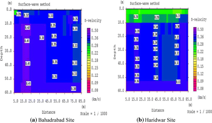
Two-Dimensional shear wave velocity profile using MASW test at Sites
Figure 4 shows 1-D shear wave velocity profile of all the five sites. This is based on the average value of shear wave velocity at a particular depth and shown only up to the depth of bore-hole for each site. It can be observed that the shear wave velocity for Solani Riverbed and Bhagwanpur Site are well below 170 m/s for all depths, indicating loose soil deposit at these sites whereas the shear wave velocity profiles at all other three sites indicate medium soil.
Fig. 4 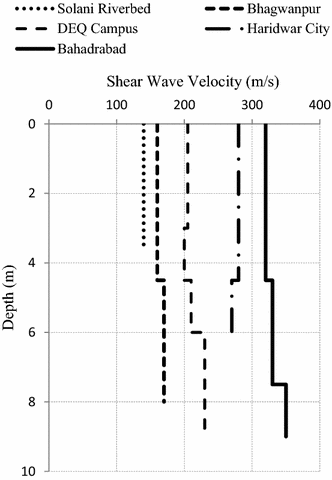
One-Dimensional shear wave velocity profile of Roorkee region sites


Laboratory Data
All the samples were examined to know their index properties according to IS: 2720 [26], including sieve analysis, i.e. grain size distribution (GSD), coefficient of uniformity (C u), coefficient of curvature (C c) and soil classification. Other properties like specific gravity, maximum and minimum void Ratio, relative density, Atterberg’s limits, etc. for all samples are also evaluated. Figure 5 shows GSD curves for all the sites which indicate that the particles are finer than 600 micron at all five sites.

Grain size distribution curves of SPT sites
At the Solani riverbed, only four samples were collected up to 3.5 m depth due to high water pressure. It can be observed from GSD shown in Fig. 5a that the more than 95 % of the particle size lies in the range of fine sand and less than 2 % are passing through 75 micron sieve for all depths. Thus the soil was classified as poorly graded sand i.e. SP. Similar, observations were made at other sites and properties are listed in Tables 2 and 3. For DEQ Campus, the samples were collected from depths 0.75, 1.5, 3.0, 4.5, 6.0, 7.5 and 9.0 m. GSD curves for samples collected from depth 0.75, 1.5, 7.5 and 9.0 m are given in Fig. 5b indicating fine sand. For the samples collected from depths 3.0, 4.5 and 6.0 m, soil classification is done based on their plasticity index (PI).
For Bhagawanpur, seven samples were collected up to 8.0 m depth. At depths 4.5 and 6.0 m, soil classification is based on PI and soil is classified as CL. For other depths, GSD are shown in Fig. 5c.
For Bhadrabad, up to 9.0 m depth, 8 SPT samples were collected different depths. It can be observed from Fig. 5d, that at the most of the depth, fine content are more than 20 %. At 4.5 and 9.0 m depth, soil samples classified as CL is based on plasticity chart.
Figure 5e shows the particle size distribution of the Haridwar city of 5 SPT samples up to 6.0 m depth which indicate that the fine contents are different at different depths. High fine contents are 35.60 and 32.20 % at depths 1.5 and 4.5 m respectively.
Results and Discussions
The average shear stresses (τ av) in soil at different depths were computed using the simplified method (Eq. 1) as well as using the ground response analysis for all the sites. For the simplified method a max equal to 0.24 g and for GRA, PGA equal to 0.2 g were considered. Figure 6 shows the plot of the average shear stress values against the depth computed using both these methods for all the five sites. It can be observed that the GRA gives greater values of shear stresses at all the depths as compared to the simplified method. Also, the difference in the shear stress values obtained using these two methods is more or less the same at all the depths; however, the percentage increase in GRA values (with respect to values of simplified method) is relatively greater at shallow depths. The same trend of result is observed for all the five sites.

Comparison of shear stresses induced due to earthquake loading using simplified method and using ground response analysis
The trend of results shown in Fig. 6 can be attributed to the fact that the shear wave velocity is a key parameter in ground response analysis while in simplified method, the total stress plays a major role (Eq. 1). Further, the difference between shear stress using these two methods is higher in Fig. 6a–c due to lower values of shear wave velocities (Fig. 4) for these sites, However this difference for Bahadrabad and Haridwar sites are smaller due to high values of shear wave velocities (Fig. 6d, e).
Shear stress causing liquefaction was evaluated using two methods i.e. laboratory and field approach discussed in “Shear Stress Required to Cause Liquefaction τ liq ” section. Figure 7 shows the variation of shear stress causing liquefaction with the depth, evaluated by these two methods. It can be observed that the shear stress causing liquefaction obtained using field approach (τ f) is consistently greater by some margin than that obtained from lab approach (τ lab) for all the cases. For example, in case of DEQ Campus site (Fig. 7b); shear stress causing liquefaction by field approach is slightly higher than that using the lab approach. The similar trend has been observed at Solani riverbed and other sites as shown in Fig. 7a–e. In Fig. 7b, c, d, the zone of clay layers have been indicated using dotted lines based on the data presented in Table 2.

Comparison of shear stresses causing liquefaction of SPT Sites based on laboratory and field tests
Figures 8, 9, 10, 11 and 12 show the factor of safety (FS) with the depth against liquefaction for all five sites. For all the sites, the FS using lab approach and using field approach are compared along the depth for two cases (a) using simplified method (b) using GRA.

Factor of safety against liquefaction by field and lab test for Solani Riverbed Site

Factor of safety against liquefaction by field and lab test for DEQ Campus Site

Factor of safety against liquefaction by field and lab test for Bhagwanpur Site

Factor of safety against liquefaction by field and lab test for Bahadrabad Site

Factor of safety against liquefaction by field and lab test for Haridwar City Site
While evaluating FS, for some depths, first liquefaction is ruled out using Chinese criteria either due to presence of clay layers and/or due to water content less than 90 % of liquid limit (Table 2). For example, for DEQ Campus from 3 to 6 m depth (Fig. 9); Bhagwanpur from 4.5 to 6.0 m depth (Fig. 10); Bahadrabad at 4.5 and 9.0 m depths (Fig. 11), the possibility of liquefaction is ruled out. In Figs. 9, 10 and 11, the dotted line is used to show this range of no liquefaction (NL), drawn on the basis of average depths of SPT layers.
In Figs. 8, 9, 10, 11, 12, it can be observed that the FS using field approach is higher than that using the lab approach for both the cases i.e. (a) using simplified method (b) using GRA. This can be attributed to the fact the shear stress required to cause liquefaction using field approach is greater than that using the lab approach (i.e. τ f > τ lab) as indicated in Fig. 7.
Value of FS using GRA is significantly smaller than that using simplified method. At most of the depths, the value of FS using GRA is almost half than that using simplified method. This holds for both the lab and field approach. This outcome is attributed to the difference in shear stress due to earthquake loading (τ av) using two methods (Fig. 6). Thus it can be concluded that for the evaluation of liquefaction potential of sites, it is very important to perform ground response analysis and simplified method may not be adequate (as it may indicate no threat of liquefaction which may actually not be true).
The similar conclusion was reported by Prakash and Guo [8] for Kushiro, Japan region. These researchers studied 24 sites with 92 profiles of sandy deposits where earthquakes have occurred. In the present study, both sandy and clayey types of soils are considered. Prakash and Guo [8] has also reported τ f is consistently marginally greater than τ lab at shallow depths and difference increases at higher depths. The same trend of results was reported in the present study for Roorkee region.
Further, the FS of safety at all the depths using GRA are less than unity at all the sites which indicate potential of liquefaction considering PGA = 0.2 g. For, Bahadrabad and Haridwar sites FS is relatively greater though still less than unity (FS < 1) using both the methods. Thus there is a clear threat of liquefaction at almost all the sites for the depths explored. These sites require ground improvement.
Comparison with Past Studies
A number of researchers evaluated liquefaction potentials of different regions, however comparison of laboratory and field results were rarely performed. Rao and Satyam [27] evaluated liquefaction potential of Delhi region using SPT test based data for seismic microzonation. Delhi region being in seismic Zone-IV has high seismic risk. Hazarika and Boominathan [28] reported liquefaction induced ground failures due to 2001 Bhuj earthquake of magnitude M W = 7.7. The performance-based liquefaction potential analysis was carried out [29] to estimate the earthquake induced liquefaction for Bangalore city, through a probabilistic approach based on SPT data. The entire range of peak ground acceleration (PGA) and earthquake magnitudes were used in the evaluation of liquefaction return period. Neupane and Suzuki [30], has performed liquefaction potential of Kathmandu Valley using SPT N-values and investigated the effects of fine on liquefaction potential. Dixit et al. [31] has evaluated the susceptibility of soil liquefaction for Mumbai city using simplified empirical procedure based on SPT test data. The liquefaction is evaluated for Mumbai city in terms of the factors of safety against liquefaction along the depths of soil profiles for different earthquakes with 2 % probability of exceedance in 50 years. Liquefaction potential index is computed by integrating the factors of safety along the depth and contour maps of liquefaction potential index of Mumbai city were presented.
Sesov et al. [32] evaluated the liquefaction potential by in situ tests and laboratory experiments in complex geological conditions. For in situ tests, SPT and CPT are used and for laboratory tests Cyclic Triaxial is employed. Tatsuoka et al. [33] used SPT data for evaluating liquefaction potential in Japan. Tokimatsu and Yoshimi [34] presented empirical correlation of soil liquefaction based on SPT N-value and fines content. In all these studies liquefaction potential is evaluated while in the present study this has been performed using both laboratory and field data.
Summary and Conclusions
The liquefaction potential of Roorkee region has been analyzed using field and laboratory tests. The factor of safety (FS) against liquefaction is determined using results of field and lab tests using two approaches i.e. (a) simplified method and (b) ground response analysis. It was observed that there are significant differences in the results from different approach. Following conclusions can be drawn based on the analyses performed:
-
1.
The average shear stress (τ av) induced due to earthquake loading using GRA method is significantly greater than that using simplified method at all depths.
-
2.
The shear stresses causing liquefaction (τ liq) using field tests are marginally greater than that using laboratory tests.
-
3.
The FS for all the sites using field tests are marginally greater than that using laboratory tests.
-
4.
The FS for all the sites using GRA method is almost half of that using simplified method at most of the depths. Thus indicating that the analysis performed using simplified method may not be adequate.
-
5.
The analyses indicate that there is clear threat of liquefaction at all the sites in the considered depth assuming water table at the ground. Thus the sites require ground improvement.
This study presents the liquefaction potential of Roorkee region which is not reported in the literature. Based on the outcome of the analyses, it is recommended that ground response analyses shall be carried out for all important projects as the simplified method may not be adequate. Though this outcome is based on limited data presented here and may require further investigation. The present study has direct practical application for the design of structures and foundations in the Roorkee region.
References
Hamada M (1992) Large ground deformations and their effects on lifelines: 1964 Niigata earthquake case studies of liquefaction and lifelines performance during past earthquake. Technical Report: NCEER-92-0001, vol 1, Japanese case studies, National Centre for Earthquake Engineering Research, Buffalo
Seed HB, Idriss IM (1971) Simplified procedure for evaluating soil liquefaction potential. J Soil Mech Found Div ASCE 97(SM9):1249–1273
Seed HB (1979) Soil liquefaction and cyclic mobility evaluation for level of ground during earthquakes. J Geotech Eng ASCE 105(GT2):201–255
Seed HB, Idriss IM, Arango I (1983) Evaluation of liquefaction potential using field performance data. J Geotech Eng ASCE 109(GT3):458–482
Seed HB, Tokimatsu K, Harder LF, Chung R (1985) Influence of SPT procedure in soil liquefaction resistance evaluation. J Geotech Eng ASCE 111(GT12):1425–1445
Ishihara K (1993) Liquefaction and flow failure during earthquakes: the 33rd Rankine Lecture. Geotechnique 43(3):351–415
Fear CE, McRoberts EC (1995) Reconsideration of initiation of liquefaction in sandy soils. J Geotech Eng ASCE 121(GT 3):249–261
Prakash S, Guo T (1999) In-Situ liquefaction resistance of sands. In: Proceedings of the international workshop on the physics and mechanics of soil liquefaction. Balkema Rotterdam ISBN: 9058090388, pp 335–340
Youd TL, Idriss IM (ed) (1997) Proceedings for the NCEER workshop on evaluation of liquefaction resistance of soils. Technical Report: NCEER-97-0022 National Center for Earthquake Engineering Research State, University of New York, Buffalo
Youd TL, Idriss IM, Andrus RD, Arango I, Castro G, Christian JT, Dobry R, Finn WDL, Harder LF Jr, Hynes ME, Ishihara K, Koester JP, Liao SC, Marcuson WF III, Martin GR, Mitchell JK, Moriwaki Y, Power MS, Robertson PK, Seed RB, Stokoe KH II (2001) Liquefaction resistance of soils: summary report from the 1996 NCEER and 1998 NCEER/NSF workshops on evaluation of liquefaction resistance of soils. J Geotech Geoenviron Eng ASCE 127(10):817–833
Cetin KO, Seed RB, Der Kiuregian A, Tokimatsu K, Harder LF, Kayen RE, Moss RES (2004) Standard penetration test-based probabilistic and deterministic assessment of seismic soil liquefaction potential. J Geotech Geoenviron Eng ASCE 130(12):1314–1340
Idriss IM, Boulanger RW (2006) Semi-empirical procedures for evaluating liquefaction potential during earthquakes. Soil Dyn Earthq Eng 26:115–130
Boulanger RW, Wilson DW, Idriss IM (2012) Examination and reevaluation of SPT based liquefaction triggering case histories. J Geotech Geoenviron Eng ASCE 138(8):898–909
Prakash S (1981) Soil dynamics. McGraw-Hill Company, New York
Choudhary SS, Maheshwari BK, Kaynia AM (2010) Liquefaction resistance of Solani sand under cyclic loads. In: Proceedings of the Indian geotechnical conference, Bombay, pp 115–118
Maheshwari BK, Patel AK (2010) Effects of non-plastic silts on liquefaction potential of Solani sand. Geotech Geol Eng 28(5):559–566
Maheshwari BK, Singh HP, Saran S (2012) Effects of reinforcement on the liquefaction resistance of Solani sand. J Geotech Geoenviron Eng ASCE 138(7):831–840
IS 1893 (Part-1) (2002) Criteria for earthquake resistance design of structures: general provisions and buildings. Bureau of Indian Standards (BIS) New Delhi
Kirar B, Maheshwari BK (2015) Dynamic properties of soils at large strains in Roorkee region using field and laboratory tests. In: Review Geotechnical Testing Journal, ASTM submitted Nov 2015
Kramer SL (1996) Geotechnical earthquake engineering. Prentice Hall Inc., Upper Saddle River
Bardet JP, Ichii K, Lin CH (2000) EERA A computer program for equivalent linear earthquake site response analysis. Department of Civil Engineering, University of Southern California, USA
PESMOS: Program for Excellence in Strong Motion Studies (2015) Dept Earthquake Eng, IIT Roorkee India. http://pesmos.in/2011/?page_id=38. Accessed 31 July 2015
Peck RB, Hansen WE, Thornburn TH (1974) Foundation engineering, 2nd edn. John Wiley and Sons Inc., New York
Seed HB, Idriss IM (1982) Ground motions and soil liquefaction during earthquakes. Earthquake Engineering Research Institute Monograph, Oakland
IS 2131:1981 Indian standard method for standard penetration test for soils. 3rd Reprint March-1997, Bureau of Indian Standards (BIS) New Delhi
IS 2720 (Part-IV) (1985) Indian standard methods of test for soils-grain size analysis. 2nd Reprint 1994, Bureau of Indian Standards (BIS) New Delhi
Rao KS, Satyam DN (2007) Liquefaction studies for seismic microzonation of Delhi region. Curr Sci 92(5):646–654
Hazarika H, Boominathan A (2009) Liquefaction and ground failures during the 2001 Bhuj earthquake India. In: Kokusho T (ed) Earthquake geotechnical case histories for performance-based design. Taylor & Francis Group, London, pp 201–226
Vipin KS, Sitharam TG, Anbazhagan P (2010) Probabilistic evaluation of seismic soil liquefaction potential based on SPT data. Nat Hazards 53(3):546–560
Neupane R, Suzuki K (2011) Liquefaction potential analysis of Kathmandu valley. Research Report of Department of Civil and Environmental Engineering, Saitama University, Japan 37:9–16
Dixit J, Dewaikar DM, Jangid RS (2011) Assessment of liquefaction potential index for Mumbai City. Nat Hazards Earth System Sci 12:2759–2768
Sesov V, Edip K, Cvetanovska J (2012) Evaluation of the liquefaction potential by in-situ tests and laboratory experiments in complex geological conditions. In: Proceedings 15th world conference earthquake engineering Lisbon, Portugal
Tatsuoka F, Iwasaki T, Tokida K, Yasuda S, Hirose M, Imai T, Konno M (1980) Standard penetration tests and soil liquefaction potential evaluation. Soils Found 20(4):95–111
Tokimatsu K, Yoshimi Y (1983) Empirical correlation of soil liquefaction based on SPT N-value and fines content. Soils Found 23(4):56–74
Acknowledgments
For this research the first author was supported by MHRD, Government of India Fellowship. This support is gratefully acknowledged.
Author information
Authors and Affiliations
Corresponding author
Rights and permissions
About this article

Cite this article
Muley, P., Maheshwari, B.K. & Paul, D.K. Liquefaction Potential of Roorkee Region Using Field and Laboratory Tests. Int. J. of Geosynth. and Ground Eng. 1, 37 (2015). https://doi.org/10.1007/s40891-015-0038-y
Received:
Accepted:
Published:
DOI: https://doi.org/10.1007/s40891-015-0038-y