Waiting time distributions in the accumulating priority queue

Abstract

We are interested in queues in which customers of different classes arrive to a service facility, and where performance targets are specified for each class. The manager of such a queue has the task of implementing a queueing discipline that results in the performance targets for all classes being met simultaneously. For the case where the performance targets are specified in terms of ratios of mean waiting times, as long ago as the 1960s, Kleinrock suggested a queueing discipline to ensure that the targets are achieved. He proposed that customers accumulate priority as a linear function of their time in the queue: the higher the urgency of the customer’s class, the greater the rate at which that customer accumulates priority. When the server becomes free, the customer (if any) with the highest accumulated priority at that time point is the one that is selected for service. Kleinrock called such a queue a time-dependent priority queue, but we shall refer to it as the accumulating priority queue. Recognising that the performance of many queues, particularly in the healthcare and human services sectors, is specified in terms of tails of waiting time distributions for customers of different classes, we revisit the accumulating priority queue to derive its waiting time distributions, rather than just the mean waiting times. We believe that some elements of our analysis, particularly the process that we call the maximum priority process, are of mathematical interest in their own right.

1 Introduction

Historically, priority queues have been analyzed under the assumptions that classes of customer have fixed priorities, and that no customer from a given class is admitted to service while there are customers present from classes of higher priority. In many situations, this type of priority queueing discipline is appropriate. However, in a situation where separate service requirements are simultaneously specified for each class, there is no reason to expect that an absolute priority discipline will yield performance levels that satisfy the service requirements. For example, high-priority classes might receive better service than specified, while the service level of low-priority customers might not be adequate. It is therefore desirable to seek a modification to the classical structure, which would enable the manager of a queue to fine-tune the customer selection discipline so that the service requirements of all customer classes are simultaneously satisfied.

The simplest discipline for achieving such an objective was first proposed in 1964 by Kleinrock in [12]; it is also widely known through its presentation in [11]. He termed it the time-dependent priority queue, but as this phrase has come to mean many things, we shall refer to it as the accumulating priority queue. Kleinrock’s objective was to achieve desired ratios of stationary mean waiting times experienced by customers from the different classes. He achieved this by stipulating that customers accumulate priority as a linear function of their time in the queue, with customers from classes for whom mean waiting times should be shorter accumulating priority at a greater rate. When the server becomes free, the customer (if any) with the highest accumulated priority at that time point is the one that is selected for service. Kleinrock’s main result was a set of recursive formulae for the stationary mean waiting times of the different classes in such a queue, expressed in terms of the parameters of the arrival and service distributions involved, and the rates of accumulation. He further showed that, for a stable queue, it is possible to achieve any set of ratios of stationary mean waiting times (within a region determined by the values of these ratios in an absolute priority queue) by suitably tuning the accumulation rates. Of course, the actual values of the mean waiting times depend on the traffic intensity.

Kleinrock’s primary motivation in [12] was the scheduling of computer jobs as a function of the queue length. Ours comes from healthcare applications. Patients in many jurisdictions around the world are classified according to an acuity rating system. The performance of such systems is assessed typically in terms of compliance with a set of Key Performance Indicators (KPIs) expressed in terms of distributional tails. These KPIs specify, for each priority class, both a benchmark time standard, and a proportion of patients whose waiting times before accessing treatment should not exceed the stipulated standard. For example, as is depicted in Table 1, the Canadian Triage and Acuity Scale (CTAS) [4] formulates five priority classifications for assessment in an emergency department, each with its own time standard and compliance target for the proportion of that class’s patients that need to meet that standard. The Australasian Triage Scale [3], on which CTAS is based, likewise, has five priority classes, but with different compliance targets. Elective patients awaiting surgery or treatment are also categorized into priorities with compliance targets; we cite as particular examples hip and knee replacement priority scoring in Canada [2] and New Zealand [7], and coronary artery bypass graft surgery in New Zealand [15]. Curtis et al. [6] gave an overview of prioritisation in Australia, as well as a discussion of the Clinical Priority Assessment Criteria (CPAC) tools used in New Zealand and the Western Canada Waiting List Project (WCWL) in Canada.

Table 1 CTAS key performance indicators

A variant of the accumulating priority mechanism has been considered previously by healthcare modellers in a simulation of emergency care. Hay et al. [9] proposed a mechanism which they term “operating priority” whereby all tasks have an initial priority score which then increases as a function of time. Both the initial score and the rate of increase are functions of the patient class. The authors went on to observe that their mechanism tracks the actual behaviour of an emergency care facility better than the classical priority mechanism.

In this paper, we extend Kleinrock’s analysis to derive the stationary waiting time distribution for each class in a single-server accumulating priority queue with Poisson arrivals and generally distributed service time distributions. Our analysis involves the introduction and study of a stochastic process, the maximum priority process, that we believe is of interest in its own right.

The remaining sections proceed as follows. Following a description of our model and preliminary definitions in Sect. 2, we discuss the maximum priority process for the two-class queue in Sect. 3, and define the concept of an accreditation interval in Sect. 4. We then recall some useful results concerning the waiting time and busy period distributions in a standard first-come-first-served $M/G/1$ queue in Sect. 5 and derive expressions for the Laplace transforms of the accumulated priority of customers entering service in a two-class accumulating priority queue in Sect. 6. Section 7 contains preliminary results for a multiclass system and Sect. 8 the derivation of the waiting time distribution of customers of all classes. Section 9 contains some comments concerning an alternative derivation of the waiting time distribution for the lowest priority class in the general multiclass case. Section 10 shows how to utilise our results to design an efficient method for simulating an accumulating priority queue, while Sects. 11 and 12 present a numerical example and some comments and suggestions for further research, respectively.

2 Our model

We consider a single-server queue with Poisson arrivals and general service times. Customers of class $i,\ i=1, 2, \ldots ,N$ arrive at the queue as a Poisson process with rate $\lambda _i$. Upon arrival, a customer of class $i$ starts accumulating priority at rate $b_i$, where $b_1 > b_2 > \ldots > b_N$. Thus, if a customer of class $i$ arrives at time $t$ and is still in the system at time $t' > t$, their accumulated priority at time $t'$ is $b_i (t' - t)$. When a customer completes service, the next customer to be served is the one with the greatest accumulated priority at that instant.

Figure 1 plots the accumulated priorities of customers against time for the sample path of such a process with two classes and priority factors $b_1 = 1, b_2 = 0.5$. The arrival instants are those points (1, 3, 10, 15, 17) where the priority functions are initiated. The departure instants (14, 21, 23, 26, 31) are marked by vertical lines. The priority function for the customer that is in service (if any) is highlighted, and we see that the sequence of services is: class 1, class 2, class 1, class 1, and class 2. In this plot we see examples of both a class 2 arrival being served before a class 1 customer that arrived while it was waiting (at time 14), and of a later class 1 arrival overtaking an earlier class 2 arrival and being served first (at time 23).

Fig. 1

Accumulated priorities

Let $\mathbf{T }= \{T_n; n = 1,2, \ldots \}$ be the process of inter-arrival times at the queue, with $T_1$ being the time of the first arrival and $\tau _n = \sum _{k=1}^n T_k$ being the time of the $n^{th}$ arrival. For each $n$, let $\chi (n)$ be the class and $X_n$ the service time of the $n^{th}$ customer, with ${\varvec{\chi }} = \{\chi (n); n = 1,2, \ldots \}$ and $\mathbf{X} = \{X_n; n = 1,2, \ldots \}$.

Let $X^{(i)}$ be a random variable having the service time distribution of a class $i$ customer, with mean $1/\mu _i$, distribution function $B^{(i)}$, and Laplace-Stieltjes transform (LST) $\widetilde{B}^{(i)}(s) = E(e^{-sX^{(i)}})$, defined in the right complex half-plane and for at least some $s$ with $\mathfrak {R}(s)< 0$. Under the assumption that the interarrival times and service processes are independent of one another, and that the queue is stable (that is, $\rho =\sum _{i=1}^N \rho _i = \sum _{i=1}^N \lambda _i/\mu _i < 1$), we wish to find the distribution of the stationary queueing time (that is, waiting time prior to service) for customers of different classes. Throughout the paper, we shall denote by $\widetilde{F}$ the LST of a random variable with distribution function $F.$

3 The maximum priority process for the two-class accumulating priority queue

In this section we present a detailed discussion of the two-class accumulating priority queue, before considering the more general multiclass accumulating priority queue.

We begin with the accumulating priority function for the $n$th customer, defined by

$$\begin{aligned} V_n(t) = \left\{ \begin{array}{ll} b_{\chi (n)} [ t - \tau _n] &{} \quad \hbox {if} \quad \tau _n < t \\ 0&{}\quad \hbox {otherwise.} \end{array} \right. \end{aligned}$$

Note that, here we have permitted priority to continue accumulating for a customer during their service and after their departure. This is simply for ease of notation.

Although arrivals of a given class are served in the order in which they arrived, this is no longer a FIFO queue. Define $n(m)$ to be the position in the arrival sequence of the $m$th customer to be served. So, for instance, if the 10th arrival was actually the 4th to be served, then $n(4) = 10$. When the system starts empty, we see that $n(1) = 1$, and, more generally, if the $k$th customer to arrive is the first customer in a busy period then $n(k) = k$. Note that if $n(m) > m$ then the $m$th customer to be served must be of class 1, whereas if $n(m) < m$ then the $m$th customer to be served must be of class 2. If $n(m) = m$, then the customer can be of either class.

Let $C_n$ be the time at which service commences for the $n$th arrival (so that the time at which the $m^{th}$ service commences is given by $C_{n(m)}$), and $D_n = C_n + X_n$ be the departure time of the $n$th customer to arrive, with $\mathbf{C} = \{C_n; n = 1, 2,\ldots \}$ and $\mathbf{D} = \{D_n; n = 1,2,\ldots \}$. The departure of the $m$th customer to be served occurs at time $D_{n(m)}$. If there are no other customers queued at this time, then the busy period ceases and the next customer to arrive commences service immediately. Otherwise, the queueing discipline chooses the customer with the highest priority from those that are yet to be served. So we can write

$$\begin{aligned} n(m+1) = \min \{ {\arg \max }_{n \notin \{n(i): 1 \le i \le m\}} V_n (D_{n (m)}) \}. \end{aligned}$$

(1)

The minimum here covers those instances where the $m$th departure instant coincides with the end of a busy period, at which time the priority function for all unserved customers is zero. We have $C_{n(1)} = C_1 = T_1 = \tau _1$ and, for $m > 1$, $C_{n(m+1)} = \max \{D_{n(m)}, \tau _{n(m+1)}\}$.

We are now ready to define the maximum priority process for the accumulating priority queue in the two-class case.

Definition 3.1

The maximum priority process $\mathbf{M} = \{(M_1(t), M_2 (t)), t \ge 0 \}$ for the accumulating priority queue in the two-class case is defined as follows.

• 1. If the queue is empty at time $t$, that is if $t \in [D_{n(m)},\tau _{n(m+1)})$ for some $m$, then $M_1(t)=M_2(t) = 0.$

• 2. At the sequence of departure times $\{D_{n(m)}, m = 0,1,2, \ldots \}$,

  $$\begin{aligned} M_1(D_{n(m)})&= \max _{n \notin \{n(i): 1 \le i \le m\}} V_n (D_{n (m)}) \\ M_2(D_{n(m)})&= \min \{M_1(D_{n(m)}), M_2(C_{n(m)}) + b_2 X_{n(m)}\}. \end{aligned}$$

• 3. For $t \in [C_{n(m)},D_{n(m)})$ with $\max _{\{m: D_{n(m)} > t\} } V_{m} (t) > 0$ (that is, when there are customers present in the queue),

  $$\begin{aligned} M_i (t) = M_i (C_{n(m)}) + b_i (t - C_{n(m)}). \end{aligned}$$

  (2)

The idea underlying this process is that, for each time $t\ge 0$ which is not a departure time, it gives the least upper bound for the priorities of queued customers from each class, given only knowledge of the times at which previous customers entered service, and their accumulated priority at these times. At departure times, $M_1(t)$ is determined by the maximum of the accumulated priorities of customers still in the queue, which is exactly the accumulated priority of the customer just commencing service.

Figure 2 plots $M_1(t)$ and $M_2(t)$ (in bold) against $t$ for the sample path of Fig. 1, superimposed on the priority functions $V_n(t)$.

Fig. 2

Maximum priorities

It is obvious that the $M_1(t)$ bounds the accumulated priorities of class 1 customers, since it bounds the accumulated priorities for all customers in the queue. Note that $t - M_1(t)/b_1$ is also a lower bound on the possible arrival times of the class 1 customers who are still in the queue.

To see that $M_2(t)$ bounds the accumulated priorities of class 2 customers, we consider the sample path behaviour in more detail. Assume that the queue starts empty, and that the first busy period commences at time $\tau _1$ with $M_1(\tau _1) = M_2(\tau _1) = 0$. At any time $t$ during the first service time, any queued customers of class 2, which must necessarily have an arrival time later than $\tau _1$, must have accumulated priority less than $b_2(t - \tau _1)$.

Now consider the first departure time, $D_{n(1)} = D_1 = \tau _1 + X_1$. Denoting the largest priority of all the customers in the queue by $V$, one of the following three conditions must hold:

• 1. The queue is empty, and we set $M_1(t)=M_2(t)=0$ until the next arrival.

• 2. $V\ge M_2(D_{n(1)}-)$ as depicted in Fig. 3a. In this case, since $M_2(D_{n(1)}-)$ is an upper bound on the priority of class 2 customers, the customer with priority $V$ must necessarily be of class 1. At any time $t$ during the next service, the least upper bound on the priority of class 1 customers is $V+b_1(t-D_{n(1)})$, while the priority of the class 2 customers is bounded by $M_2(D_{n(1)}-)+b_2(t-D_{n(1)}) = b_2(t-\tau _1)$.

• 3. $V<M_2(D_{n(1)}-)$ as depicted in Fig. 3b. In this case, the customer with priority $V$ can be of either class. At any time $t$ during the next service, the least upper bound on the priority of class 1 customers is $V+b_1(t-D_{n(1)})$, and the priority of the class 2 customers is bounded by $V+b_2(t-D_{n(1)})$.

  Fig. 3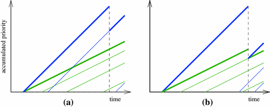

  

  The process $M_2(t)$ at departure times

At later departure times within the first busy period there are again three possible outcomes as above, and the argument follows in a very similar fashion, except that the expressions for $M_1(t)$ and $M_2(t)$ may be more complex as given in Definition 3.1 above. In each case we can infer bounds on the earliest possible arrival times of either class 1 or class 2 customers from the accumulated priority of the customer that enters service.

The expressions that we have given above for various quantities hold regardless of distributional assumptions for the queue. However, the assumption that the arrival process is Poisson leads to a result that we can exploit to show that the distributional properties of the maximum priority process are preserved if we do not keep track of the accumulated priority of the waiting customers, but instead sample the maximum such priority at each departure point. To express this, let ${\mathcal M}(t)\equiv \sigma \{(M_1(u),M_2(u)), u \in [0,t]\}$ be the filtration generated by the maximum priority process up to time $t$.

Theorem 3.2

Let $t \in [0,\infty )$.

• 1. Conditional on $\mathcal{M}(t)$, the accumulated priorities $\{V^{i}_k(t),k=1,2\ldots \}$ of the customers still waiting from class $i;\ i=1, 2$ are distributed as independent Poisson processes with rate $\lambda _i/b_i$ on the intervals $[0,M_i(t))$.

• 2. Conditional on $\mathcal{M}(t)$, the accumulated priorities $\{V_k(t),k=1,2,\ldots \}$ of all customers still present in the queue are distributed as a Poisson process with piecewise constant rates zero on the interval $[M_1(t),\infty )$, $\lambda _1/b_1$ on the interval $[M_2(t),M_1(t))$ and $\lambda _1/b_1+\lambda _2/b_2$ on the interval $[0,M_2(t))$.

• 3. A waiting customer with priority $V \in [0,M_2(t))$ is of class $1$ with probability $\lambda _1b_2/(\lambda _1b_2+\lambda _2b_1)$ independently of the class of all other customers present in the queue.

• 4. The statements 1–3 above also hold at any random time $T$ that is a stopping time with respect to $\mathcal{M}(t)$.

Proof

If there is no customer in service at time $t$, the statements of the theorem hold vacuously.

• 1. Otherwise, let $\tau < t$ be the time at which the current service commenced. Since $(M_1(t),M_2(t))$ are deterministic functions of $(M_1(\tau ),M_2(\tau ))$, $\mathcal{M}(t)$ contains the same information as ${\mathcal M}(\tau )$. Furthermore, the maximal priority of any class $i$ customer queued at time $\tau$ was $M_i(\tau )$, which means that such customers must have arrived after time $\tau - M_i(\tau )/b_i$. The arrival times $\{C_k^i,k=1,2,\ldots \}$ of class $i$ customers in the queue at time $t$ (who either had priority less than $M_i(\tau )$ at time $\tau$ or arrived in the queue in the interval $(\tau ,t]$) occur as a Poisson process with rate $\lambda _i$ on the interval $(\tau - M_i(\tau )/b_i,t]$, independently of any random variable that is measurable with respect to ${\mathcal M}(\tau )$. The priorities of these customers at time $t$ are such that $V_k^i(t) = b_i(t-C_k^i)$, and so these occur as a Poisson process with parameter $\lambda _i/b_i$ on the interval $[0,M_i(\tau )+b_i(t-\tau )) = [0,M_i(t))$.

• 2. The process of accumulated priorities $\{V_k(t),k=1,2,\ldots \}$ of all customers still present in the queue at time $t$ is the superposition of the processes of accumulated priorities $\{V^{i}_k(t),k=1,2\ldots \}$ of the customers of class $i$ still present in the queue at time $t$. These processes are independent, since the arrival processes of class $1$ and $2$ customers are independent Poisson processes, and the result follows from the well-known property that a superposition of independent Poisson processes is Poisson with rate equal to the sum of the individual rates (see, for example, [10, Exercise 2.1]).

• 3. This also follows from the well-known property that the individual processes in a superposition of independent Poisson processes have the same law as independent thinnings of the overall process [10, Exercise 2.2].

• 4. The extension to random times that are stopping times follows from the strong Markov property of the Poisson process. $\square$

We conclude this section by recording formal expressions for $M_1(t)$ and $M_2(t)$ in terms of the arrival and service processes. Let

$$\begin{aligned} {N_S}(u) = \min \{j: \sum _{m=1}^j X_{n(m)} >u \}. \end{aligned}$$

(3)

This can be interpreted as the maximum number of customers who would have commenced service by time $u$ under the permutation $n$ if the system had not experienced any idle time. Let $L(t), t \ge 0$ be the cumulative idle time experienced by the server up to time $t$ given by

$$\begin{aligned} L(t) = \int \limits _0^t I [ \sum _{k=1}^{N_S(u - L(u))} T_k \ge u] du. \end{aligned}$$

(4)

We define $K(t)=N_S(t-L(t))$ to identify the index of the current service, if one is under way. That is, if the server is busy at time $t$ then the current service is the $K(t)$th, whereas if the server is idle at time $t$, then exactly $K(t)-1$ services have been completed and the next, at the beginning of the next busy period, will be the $K(t)$th. Then, for $t > \tau _{n(K(t))}$,

$$\begin{aligned} M_1(t)&= b_{\chi (n(K(t)))} [ C_{n(K(t))} - \tau _{n(K(t))} ] + b_1 [t - C_{n(K(t))}] \end{aligned}$$

(5)

$$\begin{aligned} M_2(t)&= \min \left\{ b_{\chi (n(K(t))}[C_{n(K(t))} - \tau _{n(K(t))}], M_2(D_{n(K(t)-1)}) \right\} \nonumber \\&+\, b_2 [ t - C_{n(K(t))}] \end{aligned}$$

(6)

with $M_1(t) = M_2(t) = 0$ if $t \le \tau _{n(K(t))}$.

4 Accredited customers and accreditation intervals

We shall refer to those class 1 customers in the queue with accumulated priority at time $t$ that lies in the interval $[M_2(t),M_1(t))$ as accredited (at level 1), which we shall abbreviate to just accredited when there is no chance of confusion. Customers with priority in the interval $[0,M_2(t))$ are unaccredited or non-accredited.

Once a class 1 customer becomes accredited, they remain accredited until they enter service, since their priority is increasing at rate $b_1$, whereas $M_2(t)$ is increasing at rate $b_2 < b_1$. Thus, since $M_2(t)$ bounds the accumulated priority for class 2 customers, accredited class 1 customers are guaranteed service before any waiting class 2 customer.

A customer who enters service without being accredited can be of either class 1 or class 2. The service of such a customer will be followed by a sequence (possibly of length zero) of service times for accredited class 1 customers, before the next non-accredited customer is served, or the busy period ends. We shall refer to such an interval, consisting of the service time of a non-accredited customer followed by a sequence of service times of accredited class 1 customers as an accreditation interval (at level 1). A busy period for the queue can be broken into a sequence of accreditation intervals, and it is these intervals that we will study in greater detail in this section.

We begin with some observations about the process $M_2(t)$ and accreditation intervals.

Remark4.1

• 1. The periods where $M_2(t)=0$ correspond to idle periods of the queue. Thus, the durations of these periods are independent and exponentially distributed with parameter $\lambda _1+\lambda _2$. Furthermore, the stationary probability that $M_2(t) = 0$ is $1-\rho$.

• 2. Consider a customer with priority $v\in [0,M_2(t))$ at time $t$. Such a customer can be either a customer of class 2, in which case its waiting time has been $v/b_2$, or an unaccredited customer of class 1, in which case its waiting time has been $v/b_1$.

• 3. Theorem 3.2(2) tells us that, at time $t$ during a busy period, the priorities of customers lying in the interval $[0,M_2(t))$ are distributed according to a Poisson process with rate $\lambda _1/b_1 + \lambda _2/b_2$. These priorities are generated by a mixture of class 1 customers that have been arriving at rate $\lambda _1$ over the time interval $(t - M_2(t)/b_1,t]$ and accumulating priority at rate $b_1$, and class 2 customers that have been arriving at rate $\lambda _2$ over the time interval $(t - M_2(t)/b_2,t]$ and accumulating priority at rate $b_2$. Nonetheless, the distribution of the priorities at time $t$ is the same as if customers had arrived in a Poisson process with rate $\lambda _2+\lambda _1b_2/b_1$ over the whole interval $(t - M_2(t)/b_2,t]$ and had all been accumulating priority at rate $b_2$.

• 4. The customer who initiates a busy period, and thus the first accreditation interval in a busy period, is of class 1 with probability $\lambda _1/(\lambda _1+\lambda _2)$, and their accumulated priority at this time is 0. By Theorem 3.2(3), the first customer in all other accreditation intervals during the busy period is of class 1 with probability $\lambda _1b_2/(\lambda _1b_2+\lambda _2b_1)$, and their accumulated priority $v$ at this time is, almost surely, strictly greater than zero.

The maximum priority process during an accreditation interval has the form depicted in Fig. 4, which can be described as follows.

Fig. 4

An accreditation interval

• At time $t_0$, the accreditation interval commences when an initiating, non-accredited customer of class 1 or 2 with accumulated priority $V_\mathrm{init}$ moves into service. Note that $M_1(t_0) = M_2(t_0) = V_\mathrm{init}$.

• If a customer completes service at time $t$, the accreditation interval continues as long as there is at least one remaining customer that has become accredited, which is of necessity of class 1 with priority greater than $V_\mathrm{init} + b_2 (t-t_0)$. This customer moves into service, with service time distribution $B^{(1)}$. If there are no accredited customers, the accreditation interval finishes. If there are non-accredited customers present in the queue with priority less than $V_\mathrm{init} + b_2 (t-t_0)$, the one with the highest accumulated priority will start a new accreditation interval. Otherwise an idle period starts, and the next accreditation interval will start when a customer arrives to the empty queue.

• The overall service time distribution of the customer initiating the accreditation interval depends on whether the customer is also initiating a busy period of the queue. The customer who initiates the first accreditation interval in a busy period is of class 1 with probability $\lambda _1/(\lambda _1+\lambda _2)$. The first service in this interval thus has distribution $B_0^{(2)} \equiv (\lambda _1B^{(1)}+\lambda _2B^{(2)})/(\lambda _1+\lambda _2)$. The first customer in all other accreditation intervals is of class 1 with probability $\lambda _1b_2/(\lambda _1b_2+\lambda _2b_1)$, so its service time distribution is $B_2^{(2)} \equiv (\lambda _1b_2B^{(1)}+\lambda _2b_1B^{(2)})/(\lambda _1b_2+\lambda _2b_1)$. The superscript (2) in the above notation reminds us that we are dealing with the two-class case. We associate the subscript 0 with services occurring at the beginning of a busy period, and our use of the subscript 2 is consistent with our later treatment of the multiclass case. The logic behind it is that an unaccredited customer that initiates an accreditation interval with its priority lying in the interval $[0,M_2(t))$ can be considered to be commencing its service ‘at accreditation level 2’.

The following lemma will prove useful in our study of the duration of accreditation intervals.

Lemma 4.2

During an accreditation interval, the time points $s_k$ at which customers become accredited occur according to a Poisson process with rate $\lambda _1(1-b_2/b_1)$.

Proof

Consider an accreditation interval, such as that illustrated in Fig. 4, initiated at time $t_0$ by a non-accredited customer with priority $V_\mathrm{init}$ whose service time is $T_0$. Class 1 customers who become accredited during this accreditation interval are either present at time $t_0$, as is the customer who becomes accredited at time $s_1$ in Fig. 4, or arrive subsequently, as does the customer who becomes accredited at time $s_2$ in Fig. 4.

By Theorem 3.2(1), the priorities $v_k$ of those class 1 customers still in the queue at time $t_0$ are distributed according to a Poisson process with rate $\lambda _1/b_1$ on the interval $[0,V_\mathrm{init})$. These priorities increase at rate $b_1$, so that at time $t$ they are equal to $v_k + b_1(t-t_0)$, while $M_2(t) = V_\mathrm{init} + b_2(t-t_0)$, at least during the service time of this first customer. So a waiting customer whose priority at time $t_0$ was $v_k$ will become accredited during the service time of the initiating customer at time $s_k=t_0 + (V_\mathrm{init}-v_k)/(b_1-b_2)$, provided that this time is less than $t_0+T_0$. The times $s_k$ thus occur according to a Poisson process on the interval $[t_0, \min (t_0 + V_\mathrm{init}/(b_1-b_2),t_0+T_0))$, with parameter $\lambda _1(1-b_2/b_1)$, and this Poisson process is independent of $T_0$.

On the other hand, the arrival times $c_k$ of class 1 customers who arrive subsequent to time $t_0$ occur according to a Poisson process with parameter $\lambda _1$ on $(t_0,\infty )$. A customer arriving at time $c_k$ will become accredited at time $s_k = (V_\mathrm{init} + b_1c_k - b_2t_0)/(b_1-b_2)$. If this is less than $t_0+T_0$, then the customer will become accredited during the service time of the first customer. The set of such times $s_k$ thus occurs according to a Poisson process on the interval $[t_0 + V_\mathrm{init}/(b_1-b_2),t_0+T_0)$, (if, indeed, this interval is non-empty) with parameter $\lambda _1(1-b_2/b_1)$, and this Poisson process is again independent of $T_0$.

Now, let $S_1$ be the sum of the service times of all customers who become accredited in the interval $[t_0,t_0+T_0)$. If there are no such customers, then $S_1=0$ and the accreditation interval finishes at time $t_0+T_0$. Otherwise, it will continue as the accredited customer with the highest priority moves into service. Via similar arguments to those given above, we see that customers become accredited during the interval $[t_0+T_0,t_0+T_0+S_1)$ according to a Poisson process with parameter $\lambda _1(1-b_2/b_1)$ that is independent of $T_0$ and $S_1$.

For $j\ge 2$, let $S_j$ be the sum of the service times of all customers who become accredited in the interval $[t_0+\sum _{i=0}^{j-2} S_i,t_0+\sum _{i=0}^{j-1} S_i)$. Our assumption that the queue is stable leads to the fact that, with probability one, there will be an integer $1 \le J<\infty$ for which $S_{J-1}>0$ and $S_J=0$, at which time the accreditation interval finishes. For all $j<J$, the above argument can be repeated to establish that customers become accredited during the interval $[t_0+\sum _{i=0}^{j-1} S_i,t_0+\sum _{i=0}^{j} S_i)$ according to a Poisson process with parameter $\lambda _1(1-b_2/b_1)$ that is independent of $\{S_i\}, i \le j$.

We thus conclude that the process of customers becoming accredited is a Poisson process with parameter $\lambda _1(1-b_2/b_1)$ on the interval $[t_0, t_0+\sum _{i=0}^{J-1} S_i)$. $\square$

Lemma 4.3

The durations of the accreditation intervals are independent random variables whose distributions depend on $V_\mathrm{init}$ only via $I(V_\mathrm{init}>0)$.

Proof

It was observed in the proof of Lemma 4.2 that the duration of an accreditation interval depends only on the service time of the initiating customer and the arrival and service processes of the accredited customers who arrive during the interval. The distribution of the initiating service time depends on whether $V_\mathrm{init} = 0$, in which case the initiating service time has distribution $B_0^{(2)}$, or whether $V_\mathrm{init}>0$, which ensures that the initiating service time has distribution $B_2^{(2)}$.

Observe that all the random elements that affect the length of an accreditation interval are independent of the lengths of previous accreditation intervals, and so the lengths of successive accreditation intervals are independent of each other. $\square$

We would like to find the distributions of the lengths of the two types of accreditation interval: those that initiate a busy period and those that do not. From the discussion above, and Lemma 4.2, we see that these distributions will be the same as those of the busy period of an $M/G/1$ queue with arrival rate $\lambda _1(1 - b_2/b_1)$ and service time distribution $B^{(1)}$ for all customers apart from the initiating customer, but with the initial service time in the accreditation interval having distribution $B_0^{(2)}$ if the accreditation interval is the first in a busy period and $B_2^{(2)}$ if it is the second or subsequent accreditation interval in a busy period.

We shall recall some relevant results concerning busy period and waiting time distributions for $M/G/1$ queues in the next section.

5 Waiting times and busy periods in the $M/G/1$ queue

In this section we consider an $M/G/1$ queue with arrivals occurring as a Poisson process with rate $\lambda$, service times having mean $1/\mu < \infty$ with $\lambda < \mu$ and LST $\widetilde{B}(s)$. We shall connect the ideas of the maximum waiting time process and accumulating priority in a setting without distinct classes, before returning to discussion of the two-class queue in the next section.

The standard way of deriving the distribution of the busy period or waiting times in a $M/G/1$ queue is to analyse the virtual workload process $\mathbf{U} = \{U(t); t \ge 0\}$ that measures the amount of work remaining in the queue at any time $t$; see, for example, Kleinrock [10, page 206]. In terms of the arrival and service processes, this process can be defined as

$$\begin{aligned} U(t) = \left( \sum _{n=1}^{N_A(t)} X_n - t \right) - \min _{s \le t} \left( \sum _{n=1}^{N_A(s)} X_n - s \right) \end{aligned}$$

(7)

where

$$\begin{aligned} N_A(t) = \max \left\{ j: \sum _{k=1}^j T_k \le t\right\} \end{aligned}$$

(8)

is the number of arrivals that have occurred by time $t$.

On the other hand, we can analyse waiting times via a single class analogue $W(t)$ of the two-class maximum priority process that we defined in Sect. 3. Putting the accumulation rate $b=1$, this process is zero at time $t$ if the system is empty, and otherwise is equal to the maximum possible waiting time of any customer still present in the queue at time $t$, given the history of the process up to the time that the current customer started service.

In the single-class FCFS $M/G/1$ context, this is just the time in the system of the customer currently in service. Via reasoning similar to that used in Sect. 3, this process can be expressed as

$$\begin{aligned} W(t) = \left[ t - \sum _{k=1}^{K(t)} T_k\right] ^+ = [t - \tau _{K(t)}]^+, \end{aligned}$$

(9)

where $K(t)$ is as defined previously, with the permutation $n$ set to be the identity, $n(m) = m$.

The connection between the virtual workload process and the maximum waiting time process is illustrated in Fig. 5. The waiting time $W_n$ of the $n$th customer is the left limit of the virtual workload process at the time $\tau _n$. It is also the value of the maximum waiting time process at the time that the $n$th customer goes into service, which could either be a point where the $n$th customer arrives to an empty queue or a point where the $n$th customer is already present when the $(n-1)^\mathrm{st}$ customer departs. This allows us to use known results about waiting times, obtained by analysing the virtual workload process, to analyse random variables associated with the maximum waiting time process at the points where customers go into service.

Fig. 5

The virtual workload and maximum waiting time processes for an $M/G/1$ queue

The first such known result is the expression for the LST $\widetilde{G}(s)$ of the distribution of the length of a busy period, obtained by solving the functional equation

$$\begin{aligned} \widetilde{G}(s) \equiv \widetilde{G}(s;\lambda ,B) = \widetilde{B}(s + \lambda (1 - \widetilde{G}(s))) \end{aligned}$$

(10)

(see Conway, Maxwell and Miller [5, page 150, Eq. (7)] or Kleinrock [10, equation (5.137)]). A related expression that we shall make heavy use of is the LST $\widetilde{G}_0(s)$ of the duration of a busy period initiated by a service whose LST is given by $\widetilde{B}_0(s)$ with subsequent services having LST $\widetilde{B}(s)$. This is shown in [5, page 151, equation (9)] to be given by

$$\begin{aligned} \widetilde{G}_0(s) \equiv \widetilde{G}_0(s;\lambda ,B,B_0) = \widetilde{B}_0(s + \lambda (1 - \widetilde{G}(s))) \end{aligned}$$

(11)

where $\widetilde{G}(s)$ is the solution to (10).

The second known result gives the LST of the waiting time distribution before a customer enters service in the stationary regime; see for instance Kleinrock [10, equation (5.105)], which is

$$\begin{aligned} \widetilde{W}(s) \equiv \widetilde{W}(s;\lambda ,B) = \frac{s ( 1 - \rho )}{s - \lambda (1 - \widetilde{B}(s))}. \end{aligned}$$

(12)

From Eq. (12), it follows in a straightforward manner that the LST of the stationary waiting time, conditional on it being positive, is

$$\begin{aligned} \widetilde{W}_+(s) \equiv \widetilde{W}_+(s;\lambda ,B) = \frac{( 1 - \rho )\lambda (1-\widetilde{B}(s))}{\rho (s - \lambda (1- \widetilde{B}(s)))}. \end{aligned}$$

(13)

Now consider the situation where $b$ can be any real number in the interval $(0,\infty )$ and let $M(t)$ be the maximum accumulated priority at time $t$. Then

$$\begin{aligned} M(t) = \left[ bt - \sum _{k=1}^{K(t)} b T_k\right] ^+ = [b(t - \tau _{K(t)})]^+ = bW(t), \end{aligned}$$

(14)

and we see immediately that the priority that customer $n$ has accumulated when it goes into service is $b W_n$, where the sequence $\{ W_n\}$ gives successive waiting times for the $M/G/1$ queue. It follows from Eq. (12) that in equilibrium the Laplace-Stieltjes transform of the accumulated priority at such a point of discontinuity is given by

$$\begin{aligned} \widetilde{M}(s) \equiv \widetilde{M}(s;b,\lambda ,B) = \widetilde{W}(bs) = \frac{b s ( 1 - \rho )}{bs - \lambda (1 - \widetilde{B}(bs))} = \frac{s ( 1 - \rho )}{s - (\lambda /b)(1-\widetilde{B}(bs))}.\nonumber \\ \end{aligned}$$

(15)

This last expression can also be interpreted as the LST of the waiting time in a time-dilated $M/G/1$ queue (Eq. 12) with arrival rate $\lambda /b$ and service times multiplied by a factor $b$ relative to the original queue.

The LST of the accumulated priority, conditional on it being positive, is

$$\begin{aligned} \widetilde{M}_{b+}(s) \equiv \widetilde{M}_{b+}(s;\lambda ,B) = \frac{( 1 - \rho )\lambda (1-\widetilde{B}(bs))}{\rho (bs - \lambda (1 - \widetilde{B}(bs)))}. \end{aligned}$$

(16)

6 The LST of accumulated priority in the two-class queue

We return now to discussion of the two-class queue, and to determining the LST of the stationary accumulated priorities at the time points that customers move into service. Once we have the LST for the stationary accumulated priority, we immediately also have the LST for the stationary waiting time, by a simple rescaling of the argument, since a customer of class $i$ with accumulated priority $v$ upon entry to service has waited for time $v/b_i$ in the queue.

First consider the case where service times have the same distribution for the two classes, with $B^{(1)} = B^{(2)}= B$ and common mean $1/\mu = 1/\mu _1 = 1/\mu _2$. By Lemma 4.2, customers become accredited as a Poisson process with rate $\lambda _1( 1 - b_2/b_1)$, so the duration of an accreditation interval has the same distribution as the busy period of an $M/G/1$ queue with arrivals at rate $\lambda _1(1-b_2/b_1)$ and service time distribution $B$. It then follows from expression (10) that the duration of an accreditation interval has a LST that satisfies the functional equation

$$\begin{aligned} \widetilde{\Gamma }(s) = \widetilde{B} \left( s + \lambda _1 (1 - b_2/b_1) \left( 1-\widetilde{\Gamma }(s)\right) \right) . \end{aligned}$$

(17)

We shall employ this solution of Eq. (17) in a variety of contexts, and so we write its solution in terms of its parameters as $\widetilde{\Gamma }(s;b_1,b_2,\lambda _1,B)$. Following Eq. (10), an alternative notation for this is $\widetilde{G}(s;\lambda _1 (1 - b_2/b_1), B)$.

If the distribution $B_0$ of the initial service time in the accreditation interval is different from the succeeding service times, which still have distribution $B$, then for $\widetilde{\Gamma }(s)$ satisfying (17), the length of the accreditation interval has LST given by

$$\begin{aligned} \widetilde{\Gamma }_0(s) = \widetilde{\Gamma }_0(s;b_1,b_2,\lambda _1,B,B_0)= \widetilde{B}_0\left( s + \lambda _1(1 - b_2/b_1)\left( 1-\widetilde{\Gamma }(s)\right) \right) . \end{aligned}$$

(18)

Following Eq. (11), an alternative notation for this is $\widetilde{G}_0(s;\lambda _1 (1 - b_2/b_1), B,B_0)$. Taking derivatives and putting $s=0$, or referring to Conway, Maxwell and Miller [5, page 151, Eqs. (7a), (9a)], we see that the mean duration of an accreditation interval of the form described by (17) is

$$\begin{aligned} \frac{1}{\mu -\lambda _1(1-b_2/b_1)} \end{aligned}$$

(19)

and the mean duration of an accreditation interval of the form described by (18) is

$$\begin{aligned} \frac{\mu }{\mu _0\left[ \mu -\lambda _1(1-b_2/b_1)\right] }, \end{aligned}$$

(20)

where $\mu _0^{-1}$ is the mean of $B_0$.

We would like to derive the distribution of the value $\widehat{V}$ of the accumulated priority of a customer at the point that it enters service during an accreditation interval. Suppose the accreditation interval commences at time $t_0$. Let $V_\mathrm{init} = M_1(t_0) =M_2(t_0)$ denote the initial priority level in the accreditation interval. If the accreditation interval initiates a busy period for the queue, then $V_\mathrm{init}=0$. However, if the accreditation interval does not initiate a busy period then $V_\mathrm{init} > 0$ with probability one. Then the random variable $\widehat{V}$ can be written as $\widehat{V} =V_\mathrm{init}+V$ where $V$ is any additional priority that the customer accumulates during the accreditation interval, after having accumulated priority $V_\mathrm{init}$. To calculate the distribution of $V$, we modify the delay cycle approach of Conway, Maxwell and Miller [5, p. 151] to obtain the following theorem.

Theorem 6.1

For an accreditation interval with parameters $b_1, b_2$, $\lambda _1$ and $B,$ that starts at time $t_0$ with initial priority level $V_\mathrm{init}$, let $\widehat{V} = V_\mathrm{init} + V$ denote the accumulated priority of customers at the point that their service starts.

• 1. The distribution of $V$, conditional on $V_\mathrm{init}=v$, has LST

  $$\begin{aligned} \widetilde{V}^*(s;b_1,b_2,\lambda _1,B)=\frac{(\mu - \lambda _1(1-\frac{b_2}{b_1}))(\widetilde{\Gamma }(b_2s)-\widetilde{B}(b_1s))}{(1-\frac{b_2}{b_1})(b_1s-\lambda _1(1- \widetilde{B}(b_1s)))} \end{aligned}$$

  (21)

  where $\widetilde{\Gamma }(s) = \widetilde{\Gamma }(s;b_1,b_2,\lambda _1,B)$ is the solution of the functional Eq. (17).

• 2. The random variable $V$ is independent of $V_\mathrm{init}$.

Proof

Let $S_0$ denote the service time of the customer who initiates the accreditation interval and, for $j = 0,1,2 \ldots$, recursively define $S_{j+1}$ to be the time taken to serve customers who become accredited during the interval $(t_0 + \delta _{j-1}, t_0 + \delta _j]$ where $\delta _j =\sum _{i=0}^j S_i$ and $\delta _{-1}$ is equal to zero. Note that these customers must have attained priority level $v$ during the interval $(t_0 + (1-b)\delta _{j-1},t_0 + (1-b)\delta _j]$, where $b = b_2/b_1$. We shall denote the length of this interval by $A_j$. For $j = 0,1,2, \ldots$, define $\alpha _j = (1-b)\delta _j$, $H_j$ to be the distribution function of $S_j$ and $\widetilde{H}_j(s) = E\{e^{-sS_j}\}$. By Lemma 4.2, customers become accredited according to a Poisson process with parameter $\lambda _1(1-b)$, and we readily obtain the fact that

$$\begin{aligned} \widetilde{H}_j(s) = \widetilde{H}_{j-1}(\lambda _1(1 - b)(1 - \widetilde{B}(s)). \end{aligned}$$

(22)

In a similar fashion to Conway, Maxwell, and Miller [5, pp. 152–155], consider a marked customer that attains priority level $v$ in the interval $(t_0+\alpha _{j-1},t_0+\alpha _j]$ (so becomes accredited during the interval $(t_0+\delta _{j-1},t_0+\delta _j]$), and condition upon $S_j$, the residual duration $Y$ of $(t_0+\alpha _{j-1},t_0+\alpha _j]$ at the time that the customer has priority level $v$, and the number $N$ of customers who attained priority $v$ during $(t_0 + \alpha _{j-1},t_0 + \alpha _j]$ prior to the marked customer, with the region of feasibility for $(Y,S_j)$ being $\mathcal{S} = \{(y,t):0 \le y \le (1-b)t,\ 0 \le t < \infty \}.$

Given that $Y=y$, the additional waiting time $V/b_1$ of the marked customer is equal to $y$, plus the $N=n$ service times of the customers who attain priority $v$ ahead of it in the interval $(t_0+\alpha _{j-1},t_0+\alpha _j]$, plus the difference between the time instant at the end of the interval, $t_0 + \alpha _j$, and the time instant $t_0 + \delta _j$. Thus

$$\begin{aligned} E\{e^{-sV/b_1}|S_j=t,Y=y,N=n\}&= e^{-sy} \widetilde{B}(s)^n E\{e^{-s(\delta _{j-1}+t -[\alpha _{j-1} + (1-b)t])}\}\nonumber \\&= e^{-sy} \widetilde{B}(s)^n e^{-s b t}E\{e^{-s b\delta _{j-1}}\}. \end{aligned}$$

(23)

Removal of the conditioning on $N$ yields

$$\begin{aligned} E\{e^{-sV/b_1}|S_j=t,Y=y\}=e^{-sy} e^{-\lambda _1 ((1-b)t-y)(1-\widetilde{B}(s))} e^{-sb t}E\{e^{-s b\delta _{j-1}}\}. \end{aligned}$$

(24)

To remove the conditioning on $S_j=t,Y=y,$ we apply the direct analogue to the last expression in [5, page 153], and integrate over the region ${\mathcal S}$ against the joint density $dy dH_j(t)/[(1 - b)E(S_j)]$. Denoting by $\Xi _j$ the event that the tagged arrival occurs in the interval $S_j$ and paralleling the steps in Conway, Maxwell and Miller [5], we see that

$$\begin{aligned}&E\{e^{-sV/b_1}|\Xi _j\}\end{aligned}$$

(25)

$$\begin{aligned}&\quad =\frac{E\{e^{-s b\delta _{j-1}}\}\int _{t=0}^\infty e^{-s b t} e^{-\lambda _1(1 - b)(1- \widetilde{B}(s))t}\int _{y=0}^{(1- b)t} e^{-sy} e^{\lambda _1 y(1-\widetilde{B}(s))}dy dH_j(t)}{(1-b)E(S_j)}\nonumber \\&\quad =\frac{E\{e^{-s b\delta _{j-1}}\}\int _{t=0}^\infty e^{-sb t} e^{-\lambda _1(1 - b)(1-\widetilde{B}(s))t}(1-e^{-(1-b)t(s-\lambda _1+\lambda _1 \widetilde{B}(s))})dH_j(t)}{E(A_j)(s-\lambda _1(1-\widetilde{B}(s)))}.\nonumber \\ \end{aligned}$$

(26)

Evaluation of the final integral yields

$$\begin{aligned} E\{e^{-sV/b_1}|\Xi _j\}=\frac{E\{e^{-s(S_{j+1}+b\delta _j)}\}-E\{e^{-s(S_{j}+b\delta _{j-1})}\}}{E(A_j)(s-\lambda _1(1- \widetilde{B}(s)))}. \end{aligned}$$

(27)

Letting $A=\sum _{i=0}^\infty A_i$ and $S=\sum _{i=0}^\infty S_i$, and multiplying the conditional transform (27) by the probability $P(j)=E(A_j)/E(A)=E(S_j)/E(S)$ that the marked arrival attains priority $v$ during $(t_0+\alpha _{j-1},t_0+\alpha _j]$ and summing over $j$, the intermediate terms cancel, yielding

$$\begin{aligned} E\{e^{-sV/b_1}\}=\frac{E\{e^{-sb S}\}-E\{e^{-s{S_0}}\}}{E(A)(s-\lambda _1(1- \widetilde{B}(s)))}. \end{aligned}$$

(28)

Since $S$ is just the total length of the accreditation interval, we can substitute the solution of the functional equation (17), evaluated at $s b$, for $E\{e^{-s b S}\}$, and also use (19) to observe that $E(A) = (1-b)/(\mu - \lambda _1(1-b))$. Finally, remembering that $S_0$ is the initial service time and multiplying the argument of the LST by $b_1$, because that is the rate of priority accumulation, we obtain expression (21). $\square$

In most circumstances below, the service time distribution for the customer that initiates an accreditation interval will differ from that of the customers who continue it. The result for this slight variant of (21) is given in the next theorem.

Theorem 6.2

If the initial service time distribution $B_0$ differs from the service time distribution of the subsequent customers within the accreditation interval, the LST of the priority accumulated during the interval is

$$\begin{aligned} \widetilde{V}(s;b_1,b_2,\lambda _1,B,B_0)=\frac{\mu _0(1 - \lambda _1(1-\frac{b_2}{b_1})/\mu )(\widetilde{\Gamma }_0(b_2s)-\widetilde{B}_0(b_1s))}{(1-\frac{b_2}{b_1})(b_1s-\lambda _1(1-\widetilde{B}(b_1 s)))}, \end{aligned}$$

(29)

where $\widetilde{\Gamma }_0(s) = \widetilde{\Gamma }_0(s;b_1,b_2,\lambda _1,B,B_0)$ in (18).

If $B^{(1)} \ne B^{(2)}$ then accreditation intervals are all periods of the kind considered in Eq. (18) and Theorem 6.2, with $B = B^{(1)}$. An accreditation interval starting a busy period at time $t_0$ with $M_1(t_0) = M_2(t_0) = v = 0$ has $B_0=B_0^{(2)}$. On the other hand, an accreditation interval starting in the middle of a busy period with $M_1(t_0) = M_2(t_0) = v > 0$ has $B_0 = B_2^{(2)}$. We will denote the LSTs of the distributions of the lengths of these accreditation intervals by, respectively, $\widetilde{\Theta }_0^{(1)}(s) =\widetilde{\Gamma }_0(s;b_1,b_2,\lambda _1,B^{(1)},B_0^{(2)} )$ and $\widetilde{\Theta }^{(1)}(s) =\widetilde{\Gamma }_0(s;b_1,b_2,\lambda _1,B^{(1)},B_2^{(2)})$, both interpreted as in Eq. (18).

The LST of the overall busy period distribution follows from the observation in Remark 4.1 that it can be considered as an accreditation interval with $V_\mathrm{init}=0$, arrival rate $\lambda _2 + \lambda _1b_2/b_1$, priority rates $b_2$ and 0 (rather than $b_1$ and $b_2$ respectively), and service time distributions $\Theta ^{(1)}$ and $\Theta _0^{(1)}$ (rather than $B$ and $B_0$, respectively).

Thus, we can write the LST of the distribution of the length of this busy period as $\widetilde{\Gamma }_0(s;b_2,0,\lambda _2 + \lambda _1b_2/b_1,\Theta ^{(1)},\Theta _0^{(1)})$ as defined in Eq. (18). It is readily shown, after straightforward algebra and substitutions, that the implicit equation for this busy period LST yields an expression that is identical to that for an FCFS M/G/1 queue with both classes of customers, as one would expect.

The LST of the stationary accumulated priority of the non-accredited customers at the time that they enter service, conditional on it being positive, also follows from the above observation. It is given by the accumulated priority distribution with parameters $b_2, 0, \lambda _2 + b_2\lambda _1/b_1, \Theta ^{(1)}$ and $\Theta _0^{(1)}$. That is,

$$\begin{aligned} \widetilde{V}^{(2)}(s) = \widetilde{V}(s;b_2,0,\lambda _2 + b_2\lambda _1/b_1,\Theta ^{(1)},\Theta _0^{(1)}) \end{aligned}$$

(30)

in the sense of Eq. (29). Class 2 customers must, of necessity, be non-accredited when they enter service and, by Remark 4.1, the class of such a customer is independent of its priority. Also by Remark 4.1, class 2 customers who start service with priority $v$ have been in the system for time $v/b_2$. Thus the LST of the stationary waiting time for class 2 customers is given by the weighted sum of the LSTs of zero and $\widetilde{V}^{(2)}(s/b_2)$,

$$\begin{aligned} \widetilde{W}^{(2)}(s) = (1-\rho ) + \rho \widetilde{V}^{(2)}(s/b_2). \end{aligned}$$

(31)

A class 1 customer experiences one of the following outcomes:

• 1. It arrives to an empty queue.

• 2. It arrives to a non-empty queue, and is not accredited when it enters service. Since, by Theorem 3.2(3), the class of a non-accredited customer is independent of its priority, in this case the LST of its stationary accumulated priority on entering service is $\widetilde{V}^{(2)}(s)$, given by equation (30).

• 3. It enters service during the first accreditation interval of the busy period, in which case its stationary priority has LST

  $$\begin{aligned} \widetilde{V}^{(1,0)}(s) = \widetilde{V}(s;b_1,b_2,\lambda _1,B^{(1)},B_0^{(2)}) \end{aligned}$$

  (32)

  in the sense of Eq. (29).

• 4. It enters service during an accreditation interval which is started by an unaccredited customer of either class, with priority $V_\mathrm{init}>0$, in which case the extra priority that the arriving customer accumulates above $V_\mathrm{init}$ before it enters service has LST

  $$\begin{aligned} \widetilde{V}^{(1,1)}(s) = \widetilde{V}(s;b_1,b_2,\lambda _1,B^{(1)},B_2^{(2)}) \end{aligned}$$

  (33)

  again in the sense of Eq. (29). Furthermore, this extra priority is independent of $V_\mathrm{init}$, which is distributed according to a random variable with LST $\widetilde{V}^{(2)}(s)$, because $V_\mathrm{init}$ is the priority of the non-accredited customer entering service at the beginning of the accreditation interval.

By Lemma 4.2, class 1 customers become accredited at rate $\lambda _1(1-b_2/b_1)$ when the queue is non-empty, while they arrive at rate $\lambda _1$, so the probability that an individual class 1 customer, arriving during a busy period, becomes accredited is $(1-b_1/b_2)$, while the probability that it enters service while unaccredited is $b_2/b_1$. Using the fact that class 1 customers arrive according to a Poisson process and so observe time averages, we derive the fact the stationary probability that a customer finds the queue empty is $1-\rho$, the probability that it begins its service as an unaccredited customer is $\rho b_2/b_1$. The probability that a customer is accredited is $\rho (b_1-b_2)/b_1$. To derive the probabilities of the third and fourth cases, that is whether a customer is accredited during the first accreditation interval of a busy period or a subsequent one, we need to calculate the ratio of the mean length of the first accreditation interval to the mean length of the whole busy period. By (19) and (20), this is $(1-\rho )/(1-\sigma _1)$ where $\sigma _1=\rho _1(b_1-b_2)/b_1$. So the probabilities of the third and fourth categories are

$$\begin{aligned} \frac{\rho (1-\rho )(b_1-b_2)}{b_1(1-\sigma _1)} \end{aligned}$$

(34)

and

$$\begin{aligned} \frac{\rho (\rho -\sigma _1)(b_1-b_2)}{b_1(1-\sigma _1)}, \end{aligned}$$

(35)

respectively. So we finally arrive at the conclusion that the LST of the distribution of the priority of a class 1 customer when it enters service, conditional on this being positive, is

$$\begin{aligned} \widetilde{V}^{(1)}(s)&= \frac{b_2}{b_1}\widetilde{V}^{(2)}(s) + \frac{(1-\rho )(b_1-b_2)}{b_1(1-\sigma _1)}\widetilde{V}^{(1,0)}(s)\nonumber \\&+ \frac{(\rho -\sigma _1)(b_1-b_2)}{b_1(1-\sigma _1)}\widetilde{V}^{(2)}(s)\widetilde{V}^{(1,1)}(s), \end{aligned}$$

(36)

and the LST of the waiting time is

$$\begin{aligned} \widetilde{W}^{(1)}(s) = (1-\rho ) + \rho \widetilde{V}^{(1)}(s/b_1). \end{aligned}$$

(37)

7 The multiclass accumulating priority queue

In this section, we give multiclass versions of the results developed in Sects. 3, 4, and 6, that we will be using in later sections. These results will also form the basis for an efficient method for simulating an accumulating priority queue, which we will present in Sect. 10 below.

We first define the maximum priority process $\mathbf{M} = \{(M_1(t), M_2(t),\ldots , M_N(t)\}$ for the multiclass queue.

Definition 7.1

The maximum priority process for the multiclass queue is defined as follows.

• 1. For all $k=1,\ldots ,N, M_k(t)=0$ for all times $t$ when the queue is empty.

• 2. At the sequence of successive departure times $D_{n(m)}$,

  $$\begin{aligned} M_1(D_{n(m)}) = \max _{n \notin \{n(i): 1 \le i \le m\}} V_n (D_{n (m)}), \end{aligned}$$

  (38)

  and, for $1 < k \le N$,

  $$\begin{aligned} M_k(D_{n(m)}) = \min \{M_1(D_{n(m)}), M_k(C_{n(m)}) + b_k X_{n(m)}\}. \end{aligned}$$

  (39)

• 3. For $t \in [C_{n(m)},D_{n(m)})$ with $\max _{m: D_{n(m)} > t } V_{m} (t) > 0$,

  $$\begin{aligned} M_i (t) = M_i (C_{n(m)}) + b_i (t - C_{n(m)}), 1 \le i \le N. \end{aligned}$$

  (40)

By convention, we shall also define $b_{N+1} =0$ and hence $M_{N+1}(t) = 0$ for all $t > 0$. Observe that if at the departure point $D_{n(m)}$, $M_k(D_{(n(m))}) = M_1(D_{(n(m))})$, then $M_j(D_{(n(m))}) = M_1(D_{(n(m))})$ for all $j \le k$.

A generalized version of Theorem 3.2 follows straightaway.

Theorem 7.2

Let $t \in [0,\infty )$ and ${\mathcal M}(t)\equiv \sigma \{(M_1(u),M_2(u), \ldots , M_N(u)), u \in [0,t]\}$ be the filtration generated by the maximum priority process up to time $t$.

• 1. Conditional on $\mathcal{M}(t)$, the accumulated priorities $\{V^{i}_\ell (t),\ell =1,2\ldots \}$ of the customers of class $i$ still present in the queue are distributed as independent Poisson processes with rate $\lambda _i/b_i$ on the intervals $[0,M_i(t))$.

• 2. Conditional on $\mathcal{M}(t)$, the accumulated priorities $\{V_\ell (t),\ell =1,2,\ldots \}$ of all customers still present in the queue are distributed as a Poisson process with piecewise constant rates zero on the interval $[M_1(t),\infty )$, and $\sum _{j=1}^k \lambda _j/b_j$ on the interval $[M_{k+1}(t),M_k(t))$.

• 3. A waiting customer with priority $V \in [M_{k+1}(t),M_k(t))$ is of class $i$ with probability $(\lambda _i/b_i)/(\sum _{j=1}^k (\lambda _j/b_j))$ independently of the class of all other customers present in the queue.

• 4. The statements 1-3 above also hold at any random time $T$ that is a stopping time with respect to $\mathcal{M}(t)$.

Proof

Since arrivals occur as a Poisson process, the accumulated priorities of the customers of class $k$ present in the queue at time $t$ are distributed as a Poisson process with rate $\lambda _k/b_k$ on the interval $[0, M_k(t))$. The result then follows via similar reasoning as we used in the proof of Theorem 3.2. $\square$

We shall say that a customer (which must be of class $j \le k$) is at accreditation level $k$ at time $t$ if its priority lies in the interval $(M_{k+1}(t),M_k(t)]$. Similarly, we shall say that a customer becomes accredited at level $k$ when its priority moves into the interval $(M_{k+1}(t),M_k(t)]$. An application of Lemma 4.2 yields the following as a corollary to Theorem 7.2.

Corollary 7.3

Within a busy period, the time points at which customers of class $i \le k$ become accredited at level $k$ occur as a Poisson process with rate $\lambda _i(b_i - b_{k+1})/b_i$. Thus, within a busy period, the time points at which customers of all classes $i \le k$ become accredited at level $k$ are distributed as a Poisson process with rate

$$\begin{aligned} \Lambda _k = \sum _{i=1}^k \lambda _i \frac{b_i - b_{k+1}}{b_i}. \end{aligned}$$

(41)

We say that a customer from class $j\le k$ is served at accreditation level $k$ if its priority lies in the interval $[M_{k+1}(t),M_k(t))$ when it is admitted into service. An accreditation interval at level $k$ is a period of time that starts either at the beginning of a busy period or when a customer is served at some accreditation level $\ell _1$ for $\ell _1>k$, and finishes either at the end of a busy period or when another customer is served at some accreditation level $\ell _2$ for $\ell _2>k$. Whenever a customer is served at accreditation level $k$, accreditation intervals at all levels $\ell < k$ commence. In particular, considering accreditation intervals at level 0 to be services of a single class 1 customer, an accreditation interval at level $k$ can be divided into a sequence of accreditation intervals at level $k-1$, all except the last of which finish when a customer is served at accreditation level $k$.

Figure 6 illustrates this. It depicts the maximal priority process for a three-class accumulating priority queue. Accreditations intervals at levels 1 and 2 both start at the beginning of the busy period. The entire busy period can be thought of as an accreditation interval at level 3. The fourth customer to be served also starts accreditation intervals at levels 1 and 2. The third and fifth customers to enter service start an accreditation interval at level 1, but not level 2, while the service of the second customer can be thought of as constituting an accreditation interval at level 0. Notice that, for each $k=1, 2, 3$, accreditation intervals at level $k$ consist of a sequence of accreditation intervals at level $k-1$.

Fig. 6

Accreditation intervals for a three-class accumulating priority queue

We have defined the concept of an accreditation interval at level $k$. Each one of these can be thought of as a delay cycle in the sense of Conway, Maxwell and Miller [5] that starts with the service of the initiating customer and continues as long as there are customers at accreditation levels $\ell \le k$. By Corollary 7.3, these customers arrive at rate $\Lambda _k$ and have service time distribution

$$\begin{aligned} \widetilde{\beta }_{k}(s)&= \sum _{i=1}^{k} \frac{\lambda _i (b_i - b_{k+1})}{\Lambda _{k} b_i} \widetilde{B}^{(i)}(s). \end{aligned}$$

(42)

Thus, conditional on the fact that such a delay cycle is started by a customer of class $j$, the duration of the cycle is given by

$$\begin{aligned} \widetilde{\Theta }_{j,0}^{(k)}(s)&\equiv \widetilde{G}_0(s; \Lambda _k, \beta _k, B^{(j)}) \end{aligned}$$

(43)

in the sense of (11).

The following theorem gives an expression for the stationary proportion of time that the server spends on such customers.

Theorem 7.4

The stationary probability that the server is serving a customer that commenced their service at accreditation level $k$ is

$$\begin{aligned} \rho ^{(k)}=\sum _{j=1}^k\frac{\rho _j (b_k-b_{k+1})}{b_j}. \end{aligned}$$

(44)

Proof

By Corollary 7.3, customers of class $j \le k$ become accredited at level $k$ in a Poisson process with rate $\lambda _j (b_j-b_{k+1})/b_j$, and they become accredited at level $k-1$ in a Poisson process with rate $\lambda _j (b_j-b_{k})/b_j$. Let $N_j^{(k)}(t)$ be the number of class $j$ customers served at accreditation level $k$ in the interval $[0,t]$. Then it follows that the long-term rate $\lambda _j^{(k)} \equiv \lim _{t\rightarrow \infty } N_j^{(k)}(t)/t$ is $\lambda _j (b_k-b_{k+1})/b_j$. Thus the stationary probability that the server is serving a class $j$ customer that commenced their service at accreditation level $k$ is $\rho _j^{(k)}=\rho _j (b_k-b_{k+1})/b_j$ and the stationary proportion of time the server spends on customers of all classes served at accreditation level $k$ is $\rho ^{(k)}=\sum _{j=1}^k \rho _j^{(k)}$. $\square$

8 Waiting times in the multiclass queue: the general case

In this section, we establish a recursion between the LST of the waiting time distribution for delayed customers of a given class $k$ with that of customers of class $k+1$.

Let us consider the waiting time distribution for customers of class $k$, where $1 \le k \le N-1$. Arriving customers of class $k$ are of three kinds—those who begin a busy period, those customers within a busy period who are served at accreditation level $k$, and those customers within a busy period who are served at accreditation level $\ell$ for some $\ell \ge k+1$. A proportion $1- \rho$ of the customers of class $k$ begin a busy period, and therefore experience a waiting time of zero. By Theorem 7.4, of those class $k$ customers who arrive within a busy period, a proportion $(b_k - b_{k+1})/b_k$ are served at accreditation level $k$, and the remainder, a proportion $b_{k+1}/b_k$, are served at some accreditation level $\ell \ge k+1$. Thus we can decompose the LST of the waiting time distribution for class $k$ customers so that

$$\begin{aligned} \widetilde{W}^{(k)}(s)&= (1-\rho )+\rho \widetilde{W}^{(k)}_+(s) \\ \nonumber&= (1 - \rho ) + \rho [ ((b_k-b_{k+1})/b_k)\widetilde{W}^{(k)}_ {acc}(s) + (b_{k+1}/b_k)\widetilde{W}^{(k)}_{unacc}(s) ] \end{aligned}$$

(45)

where $\widetilde{W}^{(k)}_+(s)$ denotes the LST of the class $k$ waiting time distribution, conditional on it being positive and $\widetilde{W}^{(k)}_ {acc}(s)$ and $\widetilde{W}^{(k)}_{unacc}(s)$ denote the respective LSTs of the waiting time distributions for class $k$ customers, served at accreditation level $k$ or $\ell \ge k+1$, respectively.

Similarly, let $\widetilde{V}^{(k)}_ {acc}(s)$ and $\widetilde{V}^{(k)}_{unacc}(s)$ denote the respective LSTs of the priority accumulation distributions for class $k$ customers, served at accreditation level $k$ or $\ell \ge k+1$, respectively, within a busy period, and let $\widetilde{V}^{(k)}(s)$ denote the LST of the class $k$ priority accumulation distribution, conditional on it being positive. Then

$$\begin{aligned} \widetilde{W}^{(k)}_ {acc}(s) = \widetilde{V}^{(k)}_ {acc}(s/b_k), \,\, \widetilde{W}^{(k)}_{unacc}(s) = \widetilde{V}^{(k)}_{unacc}(s/b_k), \,\, \widetilde{W}^{(k)}_+(s) = \widetilde{V}^{(k)}(s/b_k). \end{aligned}$$

Using reasoning similar to the observations in Remark 4.1, we observe that those class $k$ customers who arrive within a busy period and who are served at accreditation level $\ell \ge k+1$ will have an accumulated priority on entering service that is distributed identically to that of a class $k+1$ customer who arrives during a busy period, so that

$$\begin{aligned} \widetilde{V}^{(k)}_{unacc}(s) = \widetilde{V}^{(k+1)}(s). \end{aligned}$$

(46)

Thus, we can write

$$\begin{aligned} \widetilde{V}^{(k)}(s) = ((b_k- b_{k+1})/b_k )\widetilde{V}^{(k)}_ {acc}(s) + (b_{k+1}/b_k)\widetilde{V}^{(k+1)}(s). \end{aligned}$$

(47)

The final element required to complete the specification of $\widetilde{W}^{(k)}(s)$ is the LST of the priority accumulation distribution for class $k$ customers, served at accreditation level $k$. These are customers who enter service with priority in the interval $[M_{k+1}(t),M_k(t))$ during an accreditation interval at level $k$ that must have been initiated by a customer served at some accreditation level $\ell \ge k+1$. The length of this accreditation interval will depend on the service time distribution of the customer that initiated it. This will vary depending on whether the accreditation interval at level $k$ started at the beginning of an overall busy period or, if it started within a busy period, according to the accreditation level $\ell$ at which it started.

We begin by considering an accreditation interval at level $k-1$ that starts at the beginning of a busy period (and therefore is the first accreditation interval at level $k-1$ within an accreditation interval at level $k$ that also starts at the beginning of the busy period). The first service in both such accreditation intervals has distribution

$$\begin{aligned} \widetilde{B}_0^{(N)}(s) = \sum _{i=1}^N \frac{\lambda _i}{\lambda } \widetilde{B}^{(i)}(s) \end{aligned}$$

(48)

and the accreditation interval at level $k-1$ is continued by customers that are served at accreditation level $\ell \le k-1$. The duration of this accreditation interval thus has LST

$$\begin{aligned} \widetilde{\Theta }_{0}^{(k-1)}(s) = \widetilde{G}_0(s;\Lambda _{k-1},{\beta }_{k-1},B_0^{(N)}), \end{aligned}$$

(49)

with $\beta _{k-1}$, as defined in Eq. (42), denoting the distribution of the service times of customers served at accreditation level $\ell \le k-1$.

The services that initiate subsequent accreditation intervals at level $k-1$ within the initial accreditation interval at level $k$ have service time distribution given by the LST

$$\begin{aligned} \widetilde{B}^{(N)}_k(s) = \sum _{i=1}^{k} \frac{\lambda _i (b_k - b_{k+1})}{\Lambda _k^{(N)} b_i}\widetilde{B}^{(i)}(s), \end{aligned}$$

(50)

where $\Lambda _k^{(N)} = \sum _{i=1}^{k} \lambda _i (b_k - b_{k+1})/b_i$, and the LST of the duration of these accreditation intervals at level $k-1$ is

$$\begin{aligned} \widetilde{\Theta }_{k}^{(k-1)}(s) = \widetilde{G}_0(s;\Lambda _{k-1},{\beta }_{k-1},B^{(N)}_k). \end{aligned}$$

(51)

The expressions on the right hand side of (49) and (51) should be understood as described in Eq. (11).

Lemma 8.1

The priority accumulation distribution for customers who are served at accreditation level $k$ during an accreditation interval at level $k$ that starts at the beginning of a busy period has LST

$$\begin{aligned} \widetilde{V}^{(k,0)} (s) = \widetilde{V}(s;b_k,b_{k+1},\sum _{i=1}^k \frac{\lambda _i b_k}{b_i},{\Theta }_{k}^{(k-1)},{\Theta }_{0}^{(k-1)}) \end{aligned}$$

(52)

where the expression on the right-hand-side is evaluated by using Eq. (29).

Proof

We apply the results of Theorem 3.2, with service times in that theorem replaced by durations of accreditation intervals at level $k-1$. That is, we decompose an accreditation interval at level $k$ into a succession of accreditation intervals at level $k-1$. The first, $S_0$, will be initiated by the customer that initiates the busy period and, by the above reasoning, has a duration with LST $\widetilde{\Theta }_{0}^{(k-1)}(s)$. The remainder will be accreditation intervals at level $k-1$ initiated by a customer of class $j \le k$ who is served at accreditation level $k$. Again by the above reasoning, such a period has duration $\widetilde{\Theta }_{k}^{(k-1)}(s)$. The rate at which customers arrive that will be accredited at level $k$, but not $k-1$ is given by $\Lambda _k^{(N)}$ which can be rewritten as $(1 - b_{k+1}/b_k)\sum _{i=1}^k \lambda _i b_k/b_i$ and the result then follows by using expression (29) with the parameters $b_1$, $b_2$ and $\lambda _1$ replaced by $b_k$, $b_{k+1}$ and $\sum _{i=1}^k \lambda _i b_k/b_i$, respectively. $\square$

Now we consider accreditation intervals at level $k$ that do not initiate an overall busy period. For $j=1,\ldots , N$, define

$$\begin{aligned} \widetilde{V}^{(k,j)} (s) = \widetilde{V}(s;b_k,b_{k+1},\sum _{i=1}^k \frac{\lambda _i b_k}{b_i},{\Theta }_{k}^{(k-1)},{\Theta }_{j,0}^{(k-1)}), \end{aligned}$$

(53)

where again the second expression on the right-hand-side of (53) is evaluated by using Eq. (29).

Lemma 8.2

The priority accumulation distribution for class $k$ customers who are served at accreditation level $k$ during accreditation intervals that are not initial accreditation intervals at level $k$ of an overall busy period has LST

$$\begin{aligned} \widetilde{V}_1^{(k)}(s) = \frac{\sum _{j=1}^k \rho _j\frac{b_{k+1}}{b_j} \widetilde{V}^{(k+1)}(s)\widetilde{V}^{(k,j)}(s) + \sum _{j=k+1}^N \rho _j \widetilde{V}^{(j)}(s)\widetilde{V}^{(k,j)}(s)}{\sum _{j=1}^k \rho _j\frac{b_{k+1}}{b_j} + \sum _{j=k+1}^N \rho _j }.\quad \end{aligned}$$

(54)

Proof

The mix of customers initiating an accreditation interval at level $k$ that lies within an overall busy period is different from that for the initiating interval. In particular, the initiating customer must be served at an accreditation level $\ell \ge k+1$. Of those customers from class $j \le k$ who are served within a busy period, a proportion $(b_j - b_{k+1})/b_j$ will be served at an accreditation level $\ell \le k$, and so a proportion $b_{k+1}/b_j$ will be served at an accreditation level $\ell \ge k+1$.

Now consider the customers remaining in the system at the completion epoch of an accreditation interval at level $k$. The next customer to be served will be the one with the greatest accumulated priority. Unaccredited customers from class $j < k+1$ will have the accumulated priority distribution of a class $k+1$ customer. Customers from class $j \ge k+1$ will just have the accumulated priority distribution of a class $j$ customer.

To progress further, we need to condition on the class, say $j$, of the customer initiating the accreditation interval at level $k$. Suppose that this customer had accumulated credit $V_\mathrm{init}$ at the time they commenced service. Then as we observed earlier, the accumulated priority of a customer at the point their service commences can be written as $V_\mathrm{init} + V$, where $V$ is the additional priority accumulated after priority $V_\mathrm{init}$ is attained, which is independent of $V_\mathrm{init}$ (although the form of its distribution depends on $j$).

For a customer of class $j \ge k+1$, the LST of the accumulated credit for a customer initiating an accreditation interval at level $k$ will just be $\widetilde{V}^{(j)}(s)$. To find the LST of $V$, the argument now follows that for the initial accreditation interval, except that the length of the first accreditation interval at level $k-1$ within this accreditation interval at level $k$ now has LST $\widetilde{\Theta }_{j,0}^{(k-1)}(s)$. The lengths of later accreditation intervals at level $k-1$, within the accreditation interval at level $k$ will again have LST $\widetilde{\Theta }_{k} ^{(k-1)}(s)$. We again apply Theorem 6.2, but now with $B_0 = {\Theta }_{j,0}^{(k-1)}$. For an unaccredited customer of class $j \le k$, the LST of the accumulated credit for a customer initiating an accreditation interval for class $k$ will be $\widetilde{V}^{k+1}(s)$, and the argument then follows as for $j \ge k+1$.

Finally, we determine the probabilities of the various delay cycle types occurring. In the stationary regime, the system is idle for a proportion $(1-\rho )$ of the time. The remaining proportion of time $\rho$ when the system is busy can be divided into the following separate cases:

• 1. An arrival to an empty server induces an accreditation interval at level $k$ for all $k=1,\ldots ,N$. Arrivals to an empty server from customers of class $j=1,2,\ldots ,N$ occur at rate $\lambda _j(1-\rho )$, and the mean duration of the accreditation interval at level $k$ that such an arrival induces is $1/(\mu _j(1-\sigma _k))$, where $\sigma _k=\sum _{\ell =1}^k \rho ^{(\ell )}=\sum _{\ell =1}^k\sum _{j=1}^\ell \rho _j^{(\ell )}=\sum _{j=1}^k\rho _j (b_j-b_{k+1})/b_j$ is the stationary proportion of time that the server spends on customers served at all accreditation levels $\ell \le k$. The proportion of time occupied by accreditation intervals at level $k$ started by customers of class $j$ that arrive at the beginning of a busy period is thus

  $$\begin{aligned} \pi _{0j}^{(k)}=\frac{\rho _j(1-\rho )}{1-\sigma _k}, \end{aligned}$$

  (55)

  and, summing over $j$, the proportion of time taken up by all accreditation intervals at level $k$ that occur at the beginning of a busy period is

  $$\begin{aligned} \pi _0^{(k)}=(1-\rho )\rho /(1-\sigma _k). \end{aligned}$$

  (56)

• 2. An arrival finding a busy server must be served at accreditation level $\ell \ge k+1$ to induce a further accreditation interval at level $k$. All arrivals of classes $j>k$ that arrive to a busy system comply; their contribution due to these later cycles following the same logic as above is

  $$\begin{aligned} \pi _j^{(k)}=\rho \rho _j/(1-\sigma _k). \end{aligned}$$

  (57)

  For the remaining classes, that is where $j\le k$, a customer must be served at an accreditation level $\ell \ge k+1$ to induce a later accreditation interval at level $k$, and the contribution of such customers is

  $$\begin{aligned} \pi _j^{(k)}=\rho \rho _j(b_{k+1}/b_j)/(1-\sigma _k). \end{aligned}$$

  (58)

  Summing these two terms over $j=1,2,\ldots ,N$, we see that

  $$\begin{aligned} \sum _{j=1}^N\pi _j^{(k)}=\frac{\rho \left[ \sum _{j=1}^k\rho _jb_{k+1}/b_j+\sum _{j=k+1}^N\rho _j\right] }{1-\sigma _k}. \end{aligned}$$

  (59)

Combining these proportions, we see that

$$\begin{aligned} \sum _{j=0}^N \pi _j^{(k)}&= \rho \left[ (1-\rho )+\sum _{j=1}^k\rho _j(b_{k+1}/b_j)+\sum _{j=k+1}^N\rho _j\right] /(1-\sigma _k)\nonumber \\&= \rho \left[ \left( 1-\sum _{j=1}^k\rho _j\right) +\sum _{j=1}^k\rho _j(b_{k+1}/b_j)\right] /(1-\sigma _k)\nonumber \\&= \rho \left[ 1-\sum _{j=1}^k\rho _j(1-b_{k+1}/b_j)\right] /(1-\sigma _k)\nonumber \\&= \rho (1-\sigma _k)/(1-\sigma _k)=\rho \end{aligned}$$

(60)

as we would expect.

For $1 \le j \le N$, dividing the $\pi _j^{(k)}$ by $\rho$ and cancelling the common factor $(1-\sigma _k)$ from all terms, one arrives at the weights used in Eq. (54). $\square$

Finally, to obtain $\widetilde{V}^{(k)}_ {acc}(s)$ we need to take the appropriate mixture of $\widetilde{V}^{(k,0)} (s)$ from Lemma 8.1 and $\widetilde{V}^{(k)}_1 (s)$ from Lemma 8.2.

Theorem 8.3

$$\begin{aligned} \widetilde{V}_{acc}^{(k)}(s)= \frac{1}{\rho }\left( \pi _0^{(k)} \widetilde{V}^{(k,0)}(s)+ ( \rho - \pi _0^{(k)}) \widetilde{V}^{(k)}_1(s) \right) . \end{aligned}$$

(61)

Proof

This follows immediately from the argument in the preceding Lemma. $\square$

Lemmas 8.1 and 8.2 and Theorem 8.3, taken together, give a recursive method for finding the LST for the priority accumulation distribution for a class $k$, in terms of the LSTs of the priority accumulation distributions for classes $j > k$. The LST of the class $k$ waiting time distribution conditional on it being positive, $\widetilde{W}^{(k)}_+(s)$, can then be obtained directly as follows.

Let

$$\begin{aligned} \widetilde{W}^{(k,j)}_{acc}(s) = \widetilde{V}^{(k,j)}(s/b_k), 0\le j \le N \end{aligned}$$

(62)

denote the LST for the distribution of the delay incurred within an accreditation interval by a class $k$ customer who becomes accredited either during the initial accreditation interval for class $k$ in a busy period (the case $j=0$) or a later accreditation interval with a busy period initiated by a class $j$ service time (the case $j > 0$). Then, we have the following corollary.

Corollary 8.4

The Laplace–Stieltjes transform $\widetilde{W}_+^{(k)}, k = 1,2,\ldots ,N-1$ is given by

$$\begin{aligned} \widetilde{W}_+^{(k)}(s)&= (1-b_{k+1}/b_k)\widetilde{W}^{(k)}_{acc}(s) + (b_{k+1}/b_k) \widetilde{W}^{(k+1)}_+((b_{k+1}/b_k) s) \end{aligned}$$

where

$$\begin{aligned} \widetilde{W}^{(k)}_{acc}(s)&= \frac{1 - \rho }{1 - \sigma _k} \widetilde{W}^{(k,0)}_{acc}(s) + \widetilde{W}_+^{(k+1)}((b_{k+1}/b_k)s) \sum _{j=1}^k \frac{\rho _j(b_{k+1}/b_k)}{1 - \sigma _k} \widetilde{W}^{(k,j)}_{acc}(s) \\&+ \sum _{j=k+1}^N \frac{\rho _j}{1 - \sigma _k} \widetilde{W}_+^{(j)}((b_{j}/b_k)s) \widetilde{W}^{(k,j)}_{acc}(s). \end{aligned}$$

9 Waiting times in the multiclass queue: the lowest class

In this section, we derive the LSTs of the waiting time distributions for delayed customers in the lowest priority class (class $N$). The waiting time distribution for the lowest class is the starting point that we use in the recursive determination for the waiting time distributions of the higher classes presented in the previous section. While one could, of course, merely evaluate the general expressions derived in Sect. 8 in terms of a null lower priority class, as we did for the two-class case in Sect. 6, we gain further insight by an alternative approach, which exploits the fact that the lowest class is the only one incapable of overtaking any customers that it finds in the system upon arrival. This view enables us to establish that its waiting time distribution possesses a classical priority structure that the others do not.

Theorem 9.1

The waiting-time distribution for the lowest-priority class has LST

$$\begin{aligned} \widetilde{W}^{(N)}(s) = \widetilde{W}\left( s+\Lambda _{N-1} (1-\widetilde{\eta }_{N-1}(s));\Lambda ,B_{0}^{(N)}\right) \end{aligned}$$

(63)

where $\Lambda _{N-1}$ is defined in (41),

$$\begin{aligned} \widetilde{\eta }_{N-1}(s) \equiv \widetilde{G}(s;\Lambda _{N-1}, \beta _{N-1}) \end{aligned}$$

(64)

as defined in Eq. (10), and $\widetilde{W}\left( s;\lambda ,B\right)$ is the M/G/1 waiting time LST given in Eq. (12).

Proof

Before a marked customer from the lowest class enters service, all work present in the system upon arrival must be processed, as well as that brought by later arriving customers from higher classes whose priority overtakes that of the marked customer. Thus, we can treat the waiting time for the marked class $N$ customer as comprised of two components. The first is the virtual workload present upon their arrival, which in the stationary regime has the same distribution as that of the stationary waiting time in the equivalent M/G/1 queue.

By an argument similar to that used in the proof of Lemma 7.3, the instants at which customers of class $i, 1 \le i \le N-1$ overtake the marked class $N$ customer are distributed as a Poisson process with rate $\lambda _i(b_i - b_N)/b_i$. These customers will be served ahead of the marked customer, and the additional delay they introduce thus represents a “delay busy period” in the sense of Conway, Maxwell, and Miller [5, p. 151], with the arrival rate of customers equalling $\Lambda _{N-1}$. The result then follows from (11) above. $\square$

Remark 1

In the $N=2$ case, it takes a few lines of algebra to establish the equivalence of (31) and (63), but they are, indeed equivalent.

Remark 2

For appropriate values of the parameters, the waiting time distribution for class $N$ customers turns out to be identical to that of the lower-priority group in a classical priority queue with two classes; see for instance [5, p. 164, Eq. (29)]. After substitution and elementary algebra, one finds that

$$\begin{aligned} \widetilde{W}^{(N)}(s) = \frac{( 1 - \rho )(s+\Lambda _{N-1} (1-\widetilde{\eta }_{N-1}(s)))}{s - \sum _{i=1}^N\lambda _i(b_N/b_i)(1-\widetilde{B}^{(i)}(s+\Lambda _{N-1} (1-\widetilde{\eta }_{N-1}(s))))}. \end{aligned}$$

(65)

In the classical priority formulation with the notation of [5], the arrival rate of the higher priority class is $\lambda _a = \Lambda _{N-1}=\sum _{i=1}^{N-1} \lambda _i(b_i-b_N)/b_i$, while the arrival rate of the lower priority class is $\lambda _b = \sum _{i=1}^N \lambda _i b_N/b_i$.

10 An efficient simulation procedure

We present below an efficient method for simulating an accumulating priority queue. One method to simulate the system, of course, is to use a standard event-scheduling approach, where the simulation maintains a record of all customers in the queue together with their accumulated priorities. The alternative simulation method that we describe here simulates the maximum priority process. It requires only that a record be maintained of the maximal priorities for each of the classes, the length of the current service time, and the time that it commenced.

Theorem 7.2 is the basis for our alternative method of simulating the multiclass queue. The idea underlying the simulation is that at each departure instant, the class of the next customer to be served is determined by simulating the maximum accumulated priority as an observation from the non-homogenous Poisson process described in Theorem 7.2. Once the class of the next customer to be served is determined, their service time is drawn from the appropriate distribution for that class, the maximum priority processes are updated, and the simulation continues. The waiting time of a customer can be determined from the accumulated priority at the time it starts service. If the simulation of the non-homogenous Poisson process at a departure instant contains no points, then a busy period finishes, and the next busy period starts when the ensuing idle period is complete. We give a brief outline of the simulation below. Here we let $\tau _m$, $\chi (m)$, $X_m$ and $D_m$ be the arrival time, class, service time and departure time respectively of the $m$th customer to be served, for $m \ge 1$ and we put $\lambda =\sum _{i=1}^N \lambda _i$.

We begin the simulation in the usual way with an exponentially distributed random variable with mean $\lambda ^{-1}$ giving the first arrival time, $\tau _1$, letting this arrival be of class $k$ with probability $\lambda _k/\lambda , 1 \le k \le K$, and then drawing a service time $X_1$ from the appropriate distribution. Given the initial $\tau _1, \chi (1), X_1$ and $D_1 = \tau _1 +X_1$, then, for $1 \le k \le N, M_k(D_1-) = b_k X_1$.

At the $m$th service completion time $D_{m}$, for $m \ge 1$, draw an exponentially distributed random variable $E_{m,1}$ with mean $b_1/\lambda _1$. If $E_{m,1} < M_1(D_{m}-) - M_2(D_{m}-)$ then the busy period continues with service of a class 1 customer at accreditation level 1, with service time drawn from $B^{(1)}(s)$, and $M_1(D_{m}) = M_1(D_{m}-) - E_{m,1}$ and $M_i(D_{m}) = M_i(D_{m}-)$ for $i > 1$.

If $E_{m,1} > M_1(D_{m}-) - M_2(D_{m}-)$ then set $k=2$, and carry out the following loop until a new customer is generated. For each $k$, draw an exponentially distributed random variable $E_{m,k}$ with mean $(\sum _{i=1}^k\lambda _i/b_i)^{-1}$.

• 1 If $E_{m,k} < M_k(D_{m}-) - M_{k+1}(D_{m}-)$ then the busy period continues with the service of a customer at accreditation level $k$, and this customer (the $m+1^{st}$) is of class $j$, $1 \le j \le k$ with probability $(\lambda _j /b_j)/(\sum _{i=1}^k\lambda _i/b_i$). For $i \le k$, the maximal priorities become $M_i(D_{m}) = M_k(D_{m}-) - E_{m,k}$. For $i > k$, $M_i(D_m) = M_i(D_m-)$. Draw the service time for the $m+1^{st}$ customer, $X_{m+1}$ from the appropriate distribution, set $D_{m+1} = D_m + X_{m+1}$, $M_i(D_{m+1}) = M_i(D_m) + b_i X_{m+1}$, $1 \le i \le N$ and exit the loop.

• 2 If, on the other hand, $E_{m,k} > M_k(D_{m}-) - M_{k+1}(D_{m}-)$ and $k < N$ then set $k$ to be $k+1$ and return to step 1.

• 3 If $E_{m,k} > M_k(D_{m}-) - M_{k+1}(D_{m}-)$ for all $k \le N$, then the busy period has finished. The interval to the first arrival in the next busy period is generated as before, the next service and departure times are generated in the same manner as for the first customer, and the pattern above is repeated until termination.

Notice that the simulation requires only that the maximum priorities be carried forward, and that at each step the service time for a customer be generated, but not their arrival time, unless the customer initiates a busy period.

11 Numerical example

To illustrate the utility of the accumulating priority queue model, we use it to test whether suggested accumulation rates produce waiting time distributions that comply with Canadian Triage and Acuity Scale (CTAS) [4] delay targets for a particular configuration. Below, we derive the waiting time distributions for an idealized emergency ward area treating only CTAS 4 (less urgent) and CTAS 5 (non urgent) patients. Our class 1 comprises the CTAS 4 stream, with class 2 comprising the CTAS 5 stream. The CTAS 4 Key Performance Indicator (KPI) is that treatment for at least 85 % of less urgent patients should have commenced within one hour. The CTAS 5 KPI is for at least 80 % of non urgent patients to commence treatment within 2 h.

We assume that the arrival rates for both classes are the same: on average, one patient arrives from each class every 25 min. We have assumed exponentially distributed treatment times for both classes, with a common mean of 10 min. Class 1 accumulates priority at rate 1 per minute, while class 2 accumulates at rate $b<1$ per minute.

The waiting time distributions were recovered from the LST formulae presented in Sects. 5, 6, 7, 8, and 9 and via numerical inversion using the Gaver–Stehfest method [8, 16] employing 10 points. The method of Abate and Whitt [1] could equally well have been used.

We compared the waiting time distributions produced by the LST inversion with data produced by simulating the queue. The simulation produced histograms of the waiting times of a total of half a million customers over the two classes, that were virtually indistinguishable from the numerically-produced distributional curves. We report the waiting times as scaled multiples of the mean service time of 10 min, so that, for example, $t=6$ corresponds to 60 min.

Figure 7 illustrates that the KPI for CTAS 4 is met provided that the class 2 accumulation rate $b$ does not exceed a value just slightly less than 0.5. It is an interesting question how we solve the inverse problem of identifying the maximum value of $b$ such that the stated KPI is met precisely.

Fig. 7

Class 1 waiting time distribution

Figure 8 indicates that practically any priority accumulation rate $0<b\le 1$ will result in the KPI for CTAS 5 being met. As a result, rather than a unique value of $b$, there is a range of values of $b$ that is compatible with both KPIs being met. It is then open to Emergency Department administrators to choose a value of $b$ that meets some further criterion. In contrast, when the same example is rerun with the arrival rates increased by 12.5 %, there is in fact no value of $b$ for which both criteria are met.

Fig. 8

Class 2 waiting time distribution

The fact that there may be alternately an entire set of accumulation rates meeting all KPI criteria, or none at all, suggests that a variety of optimization problems can be formulated to identify the best among the feasible solutions available. This aspect is being explored by the authors in follow-up work.

12 Conclusion and discussion

A number of extensions to the model studied here spring to mind almost immediately. We have mentioned above the task of inverting the problem to identify the extremal class 2 accumulation rate $b$ in a two-class context so that a particular waiting time tail KPI is just met, and the more general problem of formulating a variety of optimization problems that select the “best” set of $b_i$s in some sense that not only meet the stated KPIs, but also optimize other appropriate objectives.

There are, in addition, a number of extensions to the basic model itself to consider. The first of these is to derive the waiting time distributions for the case where patients are assigned a strictly positive initial priority (which may depend upon their class) immediately upon arrival, rather than starting from 0. Further generalizations involve models where the priority accumulation function takes a more general form. For example, Kleinrock [13] considered a model where the priority at time $t$ of a customer who arrived at time $t_0<t$ is of the form $b_i(t-t_0)^\alpha$. Piecewise linear priority accumulation functions are also possible.

A further performance measure of interest is the joint stationary queue-length distribution of customers of all classes. We believe that this is related to the stationary distribution of the maximum priority process, the derivation of which is an interesting problem in its own right.

A multi-server variant of the present model is called for; at present, it seems to the authors that the only case that is tractable is the special case where all classes have exponentially distributed treatment times with the same mean. Finally, one can consider the case in which the lowest priority stream represents a set of scheduled tasks, to which higher priority customers appear at random. Such a model would seem to be appropriate in a surgical setting in which scheduled elective surgeries are disrupted by a stream of urgent surgeries arriving from the Emergency Department.

Addendum: At the galley proof stage the authors became aware of the paper [14] by Ramanan and Stolyar. This paper analyzes a certain “largest-weighted-delay-first (LWDF) scheduling policy”, which is related to our “accumulating priority discipline”. Specifically, the paper [14] uses a large deviations approach to compute the exponential decay rate of the stationary distribution of the maximal weighted delay experienced by a set of different customer classes under the LWDF policy, and also shows that the LWDF policy is optimal (within a large class of work-conserving scheduling policies) with respect to maximizing this exponential decay rate.

References

Abate, J., Whitt, W.: Numerical inversion of Laplace transforms of probability distributions. ORSA J. Comput. 7(1), 36–43 (1995)
Arnett, G., Hadorn, D.: Developing priority criteria for hip and knee replacement surgery: results from the Western Canada waiting list project. Can. J. Surg. 46(4), 290–296 (2003)
The Australasian Triage Scale. From the website. http://www.acem.org.au/media/policies_and_guidelines/P06_Aust_Triage_Scale_Nov_2000.eps
The Canadian Triage and Acuity Scale. From the website. http://www.calgaryhealthregion.ca/policy/docs/1451/Admission_over_capacity_AppendixA.eps
Conway, R.W., Maxwell, W.L., Miller, L.W.: Theory of Scheduling. Addison-Wesley, Reading (1967)
Curtis, A.J., Russell, C.O.H., Stoelwinder, J.U., McNeil, J.J.: Waiting lists and elective surgery: ordering the queue. Med. J. Aust. 192(4), 217–220 (2010)
Introduction to the National Clinical Priority System (CPS) for Access to Publicly Funded Hip or Knee Joint Replacement Surgery October 2007. http://www.nzoa.org.nz/content/CPAC_Prioritisation_Guidelines.eps
Gaver Jr, D.P.: Observing stochastic processes and approximate transform inversion. Oper. Res. 14, 444–459 (1966)
Hay, A.M., Valentin, E.C., and Bijlsma, R.A. (2006) Modeling Emergency Care in Hospitals: A Paradox—The Patient Should Not Drive the Process. Proceedings of the 2006 Winter Simulation Conference, pp. 439–445
Kleinrock, L.: Queueing Systems, vol. I. Theory Wiley, New York (1975)
Kleinrock, L.: Queueing Systems, vol. II: Computer Applications. Wiley, New York (1976)
Kleinrock, L.: A delay dependent queue discipline. Nav. Res. Logist. Q. 11, 329–341 (1964)
Kleinrock, L., Finkelstein, R.P.: Time dependent priority queues. Oper. Res. 15, 104–116 (1967)
Ramanan, K., Stolyar, A.: Largest weighted delay first scheduling: large deviations and optimality. Ann. Appl. Probab. 11, 1–48 (2001)
Seddon, M., Broad, J. Crengle, S., Bramley, D., Jackson, R. and White, H.: Coronary artery bypass graft surgery in New Zealands Auckland region: a comparison between the clinical priority assessment criteria score and the actual clinical priority assigned. J. N. Z. Med. Assoc. 119(1230), U1881 (2006). http://journal.nzma.org.nz/journal/119-1230/1881/
Stehfest, H. (1970) Numerical inversion of Laplace transforms. Commun. ACM 13(1), 47–49 (Algorithm 368 with correction (October 1970), 13, No. 10)
Acknowledgments
The authors wish to thank Azaz Bin Sharif and Xin Wang for the running of the numerical examples and the preparation of graphs. We also wish to express our thanks to Donald Campbell and Keith Stockman of Monash Medical Centre in Melbourne, Australia and Mike Carter of the Centre for Healthcare Research Engineering at the University of Toronto for useful discussions related to the healthcare applications. David Stanford’s work was partly supported by his NSERC Discovery Grant. Peter Taylor would like to thank the Australian Research Council for supporting the work of all authors through Linkage Grant LP0349153 and Discovery Grant DP110101663. Ilze Ziedins is also grateful to the Science Faculty FRDF fund at the University of Auckland for supporting this research. The authors are very grateful to an anonymous referee for a very careful reading of the first draft and numerous helpful suggestions that have considerably improved the presentation of the paper.
Author information
Authors and Affiliations
Corresponding author
Rights and permissions
Open Access This article is distributed under the terms of the Creative Commons Attribution License which permits any use, distribution, and reproduction in any medium, provided the original author(s) and the source are credited.
About this article
Cite this article
Stanford, D.A., Taylor, P. & Ziedins, I. Waiting time distributions in the accumulating priority queue. Queueing Syst 77, 297–330 (2014). https://doi.org/10.1007/s11134-013-9382-6
Received:
Revised:
Published:
Issue Date:
DOI: https://doi.org/10.1007/s11134-013-9382-6