


1. Introduction
Bubbles generated by breaking waves play important roles in many air–sea exchange processes, including sea spray aerosol generation (Modini et al. Reference Modini, Russell, Deane and Stokes2013; Veron Reference Veron2015; DeMott et al. Reference DeMott2016; Erinin et al. Reference Erinin, Wang, Liu, Towle, Liu and Duncan2019), gas transfer (Banner & Peregrine Reference Banner and Peregrine1993; Farmer, McNeil & Johnson Reference Farmer, McNeil and Johnson1993; Keeling Reference Keeling1993; Melville Reference Melville1996; Liang et al. Reference Liang, Deutsch, McWilliams, Baschek, Sullivan and Chiba2013; Derakhti & Kirby Reference Derakhti and Kirby2014) and the exchange of moisture and heat (Bortkovskii Reference Bortkovskii1987), all of which have significant impacts on weather and global climate. For these and other reasons, quantifying the size-resolved creation rate and understanding the production mechanisms of bubbles in breaking waves are important subjects of ongoing research.
Prior work has shown connections between hydrodynamic turbulence and air entrainment in the transient, two-phase flow generated by a breaking wave crest. Garrett, Li & Farmer (Reference Garrett, Li and Farmer2000) argued that relatively large bubbles are entrained initially and are subsequently prone to fragmentation driven by turbulent pressure fluctuations. They showed that the bubble size spectrum resulting from a fragmentation cascade follows a  $-10/3$ power-law scaling with bubble radius, a result that has been demonstrated in laboratory and field observations (Deane & Stokes Reference Deane and Stokes2002; Leifer & De Leeuw Reference Leifer and De Leeuw2006; Rojas & Loewen Reference Rojas and Loewen2007; Blenkinsopp & Chaplin Reference Blenkinsopp and Chaplin2010) and numerical simulations (Deike, Melville & Popinet Reference Deike, Melville and Popinet2016; Wang, Yang & Stern Reference Wang, Yang and Stern2016; Yu et al. Reference Yu, Hendrickson, Campbell and Yue2019; Yu, Hendrickson & Yue Reference Yu, Hendrickson and Yue2020; Chan, Johnson & Moin Reference Chan, Johnson and Moin2021a; Chan et al. Reference Chan, Johnson, Moin and Urzay2021b; Mostert, Popinet & Deike Reference Mostert, Popinet and Deike2021). Other power-law scalings for the large bubbles are also observed. Gaylo, Hendrickson & Yue (Reference Gaylo, Hendrickson and Yue2021) studied the evolution of the bubble size distribution of large bubbles taking into account the bubble fragmentation and entrainment, and found two regimes of equilibrium local power-law scaling, which are called weak and strong injection regimes, respectively. The weak regime has the
  $-10/3$ power-law scaling, which is independent of the entrainment size distribution and consistent with the previous observations, whereas the power-law scaling for the strong injection regime shows dependence on the entrainment power-law slope. The fragmentation cascade framework (Garrett et al. Reference Garrett, Li and Farmer2000) has provided an explanation for the formation of bubbles larger than the bubble Hinze scale, which is the bubble radius at which disruptive pressure fluctuations are balanced by the stabilizing force of surface tension.
Breaking waves are known to entrain large numbers of bubbles smaller than the bubble Hinze scale (Deane & Stokes Reference Deane and Stokes2002; Leifer & De Leeuw Reference Leifer and De Leeuw2006; Blenkinsopp & Chaplin Reference Blenkinsopp and Chaplin2010; Wang et al. Reference Wang, Yang and Stern2016; Mostert et al. Reference Mostert, Popinet and Deike2021). Rivière et al. (Reference Rivière, Mostert, Perrard and Deike2021) studied bubble breakup in homogeneous and isotropic turbulence and reported that a large number of sub-Hinze-scale bubbles are produced by a non-local breakup cascade process. The wave noise spectrogram in Deane & Stokes (Reference Deane and Stokes2002) shows that sub-Hinze-scale bubbles are created at the start of the acoustically active phase, before the main cavity fragments, suggesting that there are bubble formation mechanisms operating within breaking waves beyond the turbulent fragmentation cascade (Garrett et al. Reference Garrett, Li and Farmer2000) and that at least some of these mechanisms must generate bubbles smaller than the Hinze scale. For example, the impact of a drop on the water surface can result in the production of a swarm of small bubbles through the process of Mesler entrainment, for which some work has been done both experimentally and numerically (Carroll & Mesler Reference Carroll and Mesler1981; Esmailizadeh & Mesler Reference Esmailizadeh and Mesler1986; Oguz & Prosperetti Reference Oguz and Prosperetti1989, Reference Oguz and Prosperetti1990; Pumphrey & Elmore Reference Pumphrey and Elmore1990; Thoroddsen, Etoh & Takehara Reference Thoroddsen, Etoh and Takehara2003).
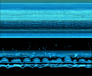
This work is motivated by the formation of bubbles due to the breakup of air cavities and spanwise filaments observed in the numerical simulations of breaking waves (see figure 1). Cavities and filaments, generically referred to as cylinders, are a ubiquitous feature of breaking waves, occurring in both spanwise and streamwise directions (Kiger & Duncan Reference Kiger and Duncan2012; Lubin & Glockner Reference Lubin and Glockner2015; Wang et al. Reference Wang, Yang and Stern2016; Lubin et al. Reference Lubin, Kimmoun, Véron and Glockner2019). The breakup of air cavities produces large bubbles, which are subsequently subject to further breakup through the Garrett et al. (Reference Garrett, Li and Farmer2000) fragmentation cascade. The stability of liquid and air jets is a classical problem that has been studied previously (see Chandrasekhar Reference Chandrasekhar2013). The unstable growth of interface waves on their boundaries, ultimately resulting in their breakup, is well known.

Figure 1. Breakup of (a) spanwise air filaments at  $t = 0.84T$ and (b) an air cavity in a simulated breaking wave crest at
  $t = 1.24T$. Wave-like perturbations appear on the interface of both structures and grow until bubbles are formed. See supplementary movie 1, available at https://doi.org/10.1017/jfm.2021.890, for an animation.
This paper presents a three-component study of the breakup of spanwise air cylinders: (1) the direct numerical simulation (DNS) of filament and cavity breakup in breaking waves, (2) a stability analysis of air cylinder breakup and (3) a grid convergence study of air cylinder breakup in a static flow field. In (1), DNS of breaking waves are performed by solving the incompressible Navier–Stokes equations on a fixed Eulerian grid using the coupled level set and volume of fluid (CLSVOF) method to capture the air–water interface. Air cylinders are identified and isolated from the breaking wave simulation domain and the most unstable mode of the unstable interface waves on the cylinders are then obtained. In (2), a theoretical analysis for the breakup of spanwise air cylinders is presented through a development of the Rayleigh–Taylor instability in cylindrical coordinates assuming that the fluid flow is stationary, incompressible and inviscid. This can also be thought of as a generalization of the Plateau–Rayleigh instability because it includes the effects of both gravity and surface tension on the stability of a fluid cylinder. A generalization is required because both these forces can be important for air cylinders in wave crests, depending on the scale of the cylinder in question. The result of the stability analysis is a generalized dispersion relation describing the relationship between the unstable modes and the cylinder radius. A comparison of the wavenumber of the most unstable modes of the interface waves on the air cylinders obtained from the DNS data with the theoretical predictions shows good agreement. In (3), the limitation of the grid resolution of the breaking wave simulations motivated us to study grid resolution effects on idealized, isolated air cylinders. The three grid resolutions chosen for the isolated air cylinders have grid sizes respectively equivalent to the same as, half of and a quarter of the breaking wave simulation grid size. The isolated cavity analysis demonstrates that there is not a grid resolution problem with the breakup of cylinders in the breaking wave simulations.
The remainder of this paper is organized as follows. We begin with the problem set-up, numerical simulation configurations and theoretical background in § 2. A generalized dispersion relation bridging the Plateau–Rayleigh instability and two-dimensional (2-D) Rayleigh–Taylor instability is also presented in § 2. The results, including data processing procedures, a comparison between the simulation results and the theoretical dispersion relation and grid convergence studies, are described in § 3. Finally, discussions and conclusions are presented in § 4 and § 5, respectively.
2. Problem set-up and theoretical background
2.1. Problem set-up
The analysis is motivated by the formation and breakup (figure 1) of an air cavity and spanwise filaments in breaking wave crests. These structures are observed in laboratory experiments (Kiger & Duncan Reference Kiger and Duncan2012) and can be identified and studied in DNS of breaking waves. The simulations are performed by solving the incompressible Navier–Stokes equations on a fixed Eulerian grid, where the air–water system is treated as a coherent system with varying physical properties. The in-house code used here implements the CLSVOF method (Sussman & Puckett Reference Sussman and Puckett2000) in capturing the air–water interface and is described in detail in Hu et al. (Reference Hu, Guo, Lu, Liu, Dalrymple and Shen2012), Liu (Reference Liu2013), Yang et al. (Reference Yang, Lu, Guo, Liu and Shen2017), Tang et al. (Reference Tang, Yang, Liu, Dong and Shen2017), Yang, Deng & Shen (Reference Yang, Deng and Shen2018) and Gao et al. (Reference Gao, Deane, Liu and Shen2021). A third-order Stokes wave with a large initial steepness in a periodic domain (Chen et al. Reference Chen, Kharif, Zaleski and Li1999; Iafrati Reference Iafrati2009; Deike et al. Reference Deike, Melville and Popinet2016; Wang et al. Reference Wang, Yang and Stern2016; Tang et al. Reference Tang, Yang, Liu, Dong and Shen2017; Yang et al. Reference Yang, Lu, Guo, Liu and Shen2017, Reference Yang, Deng and Shen2018) is adopted here. The wavelength  $L$ is
  $25~\mathrm {cm}$, which is close to that chosen by Iafrati (Reference Iafrati2009), Deike et al. (Reference Deike, Melville and Popinet2016) and Wang et al. (Reference Wang, Yang and Stern2016). The density ratio
  $\rho _a/\rho _w$ and viscosity ratio
  $\mu _a/\mu _w$ are set to
  $0.0012$ and
  $0.0154$, respectively, where
  $\rho$ is density,
  $\mu$ is dynamic viscosity and the subscripts
  $a$ and
  $w$, respectively, denote air and water.
A typical computational domain size is  $L_{x} \times L_{y} \times L_{z} = L \times L \times 0.5L$ and the largest domain size is
  $L_{x} \times L_{y} \times L_{z} = L \times L \times L$. Here
  $x$,
$x$,  $y$ and
  $z$ denote the streamwise, vertical and spanwise directions, respectively. The mean water depth is
  $d=0.5L$. The grid size is isotropic and uniform in the simulation domain and set to
  $\varDelta = L/512$. The computational time for a typical breaking wave case is approximately 100 h using 2048 cores on the supercomputer Onyx at the US Army Engineer Research and Development Center (ERDC), which uses 2.8 GHz Intel Xeon E5-2699v4 Broadwell processors, each with 22 cores, on its standard compute nodes.
The breakup of air filaments and that of an air cavity captured by the simulation are shown in figure 1. In both cases, initially small perturbations on the interface grow, forming bulges, necks and finally bubbles. The relative importance of interface curvature, gravity and surface tension to the growth of unstable interface waves depends on cylinder radius and spans what is usually referred to as the Rayleigh–Taylor instability for the largest structures, which tend to behave like a 2-D interface, to the Plateau–Rayleigh instability for the smallest structures. A new dispersion relation is required to handle cases between these two extremes and this is developed below.
2.2. The generalized dispersion relation
The filament or cavity is modelled as an infinitely long cylinder of air of radius  $R_0$ surrounded by water, with initially small wave-like perturbations growing on its boundary, as shown in figure 2. The perturbations are expressed as
  $\epsilon \exp (\omega t+\mathrm {i}kz)$, where
  $\epsilon$ is the perturbing wave amplitude,
  $\omega$ is the wave growth rate,
  $k$ is the wavenumber,
  $t$ is time and
  $\mathrm {i}$ is the imaginary unit. The fluid is assumed to be incompressible and inviscid in the stability analysis. Our study of effects of viscosity show that they are negligible for the air–water system at the scales studied here. The analysis is performed using the cylindrical coordinates
  $(r,\theta,z)$. The horizontal plane has
  $\theta =0$ or
  $\theta ={\rm \pi}$. Gravity is pointing downwards, corresponding to
  $\theta = 3{\rm \pi} /2$.

Figure 2. Geometry for the analysis in the cylindrical coordinates  $(r,\theta,z)$.
The continuity equation is
 \begin{equation} \frac{1}{r}\frac{\partial (r u_r)}{\partial r}+\frac{\partial u_z}{\partial z} = 0. \end{equation}
The Euler equations are
 \begin{equation} \rho\left(\frac{\partial u_r}{\partial t}+u_r\frac{\partial u_r}{\partial r}+u_z\frac{\partial u_r}{\partial z}\right) ={-}\frac{\partial p}{\partial r}-\rho g \sin\theta+\sigma\kappa\hat{\delta} \end{equation}
and
 \begin{equation} \rho\left(\frac{\partial u_z}{\partial t}+u_r\frac{\partial u_z}{\partial r}+u_z\frac{\partial u_z}{\partial z}\right) ={-}\frac{\partial p}{\partial z}, \end{equation}
where  $u_r$ and
  $u_z$ are the velocities along the
  $r$ and
  $z$ directions, respectively,
  $p$ is pressure,
  $g$ is gravity,
  $\sigma$ is the surface tension coefficient,
  $\kappa$ is the surface curvature and
  $\hat {\delta }$ is the Dirac delta function, which ensures that the surface tension force is imposed only on the interface. The density equation is
 \begin{equation} \frac{\partial \rho}{\partial t}+\frac{1}{r}\frac{\partial}{\partial r}\left(r\rho u_r\right)+\frac{\partial}{\partial z}\left(\rho u_z\right)=0. \end{equation}
Each of the variables  $u_r$,
  $u_z$,
  $\rho$,
  $p$ and
  $\kappa$ can be expanded as a small perturbation about an initial value:
 \begin{equation} A = \bar{A} (r) + A' (r,z,t ), \end{equation}
where  $A$ is
  $u_r$,
  $u_z$,
  $\rho$,
  $p$ or
  $\kappa$, and
  $\bar {A}$ and
  $A'$ denote the initial value and small perturbation of the variable
  $A$, respectively. We further assume that the undisturbed fluid is stationary.
Substituting (2.5) into (2.1)–(2.4) and neglecting terms of second order and higher yields the linearized equations:
 \begin{gather} \frac{1}{r}\frac{\partial (r u_r')}{\partial r}+\frac{\partial u_z'}{\partial z} = 0, \end{gather}
 \begin{gather} \bar{\rho}\frac{\partial u_r'}{\partial t}={-}\frac{\partial p'}{\partial r}-\rho' g\sin \theta +\sigma \kappa' \hat{\delta}, \end{gather}
 \begin{gather} \bar{\rho}\frac{\partial u_z'}{\partial t}={-}\frac{\partial p'}{\partial z} \end{gather}
and
 \begin{equation} \frac{\partial \rho'}{\partial t}+u_r'\frac{\partial \bar{\rho}}{\partial r} = 0. \end{equation}
The perturbation variables  $u_r'$,
  $u_z'$,
  $\rho '$ and
  $p'$ are assumed to have the form of waves:
 \begin{equation} B (r,z,t )=B_k (r) \exp(\mathrm{i}kz+\omega t ), \end{equation}
where  $B$ is
  $u_r'$,
  $u_z'$,
  $\rho '$ or
  $p'$, and
  $B_k$ is the
  $k$ component of
  $B$.
$B$.
Substituting (2.10) into (2.6)–(2.9) and eliminating  $u_{z}'$,
  $p'$ and
  $\rho '$, we obtain
 \begin{equation} \bar{\rho}k^2 u_r'=\frac{\partial}{\partial r} \left(\frac{\bar{\rho}}{r}\frac{\partial(r u_r')}{\partial r}\right) +\frac{k^2}{\omega^2}u_r' g\sin\theta\,\frac{\partial \bar{\rho}}{\partial r} +\frac{k^2}{\omega}\sigma \kappa' \hat{\delta}. \end{equation}
Away from the interface,  $\bar {\rho }$ is a constant,
  $\hat {\delta }=0$ and (2.11) simplifies to
 \begin{equation} \frac{\partial}{\partial r}\left(\frac{1}{r}\frac{\partial (r u_r')} {\partial r}\right)-k^2u_r'=0, \end{equation}
with solution
 \begin{equation} u_r' = \left\{
\begin{array}{ll} u_{r0}'
\dfrac{\textrm{I}_1(kr)}{\textrm{I}_1(kR_0)} & r\leq R_0, \\ u_{r0}' \dfrac{\textrm{K}_1(kr)}{\textrm{K}_1(kR_0)} &
r>R_0, \end{array} \right.
\end{equation}
\begin{equation} u_r' = \left\{
\begin{array}{ll} u_{r0}'
\dfrac{\textrm{I}_1(kr)}{\textrm{I}_1(kR_0)} & r\leq R_0, \\ u_{r0}' \dfrac{\textrm{K}_1(kr)}{\textrm{K}_1(kR_0)} &
r>R_0, \end{array} \right.
\end{equation}
where  $\textrm {I}_{\nu }$ and
  $\textrm {K}_{\nu }$ (
 $\nu =1$) are the first and second kinds of the modified Bessel functions, respectively, and
  $u_{r0}'$ is the perturbed velocity at the interface. The perturbed surface curvature is given by (Chandrasekhar Reference Chandrasekhar2013):
 \begin{equation} \kappa' ={-}\frac{u_r'}{R_0^2\omega} (1-k^2R_0^2 ). \end{equation}
Substituting (2.14) into (2.11) and integrating across the interface with an infinitesimal distance yields
 \begin{equation} \varDelta \left(\frac{\bar{\rho}}{r}\frac{\partial(r u_r')}{\partial r}\right) +\frac{k^2}{\omega^2} u_{r0}' g\sin\theta\,\varDelta \bar{\rho} + \frac{k^2}{\omega^2}\frac{\sigma \bar{u}_{r0}}{R_0^2} (1-k^2R_0^2 )=0, \end{equation}
where  $\varDelta (\cdot )=(\cdot )_w-(\cdot )_a$, and the subscripts
  $w$ and
  $a$ denote water and air, respectively. Substituting (2.13) into (2.15) and further simplification leads to the final result for the dispersion relation:
 \begin{equation} \omega^2\left(\rho_a\frac{\textrm{I}_0(kR_0)}{\textrm{I}_1(kR_0)} +\rho_w\frac{\textrm{K}_0(kR_0)}{\textrm{K}_1(kR_0)}\right) =k\left(g (\rho_w-\rho_a )\sin\theta+\frac{\sigma}{R_0^2} (1-k^2R_0^2)\right) . \end{equation}
Equation (2.16) permits solutions that grow exponentially in time. The length scale of the cylinder breakup processes is determined by the wavenumber of the mode that has the largest growth rate, which occurs on the top surface of the cylinder where  $\theta = {\rm \pi}/2$.
2.3. The effect of viscosity in the stability analysis
The two limiting cases, the Plateau–Rayleigh and 2-D Rayleigh–Taylor instabilities for both viscous and inviscid fluids, are discussed here for assessing the viscous effect in the stability analysis. If viscosity is present, based on Plesset & Whipple (Reference Plesset and Whipple1974) and Youngs (Reference Youngs1984), the dispersion relation for the 2-D Rayleigh–Taylor instability is approximated as
 \begin{equation} \omega^2+2\frac{\mu_w+\mu_a}{\rho_w+\rho_a}k^2\omega -\frac{\rho_w-\rho_a}{\rho_w+\rho_a}gk+\frac{\sigma k^3}{\rho_w+\rho_a}=0. \end{equation}
The dispersion relation and its derivation of the Plateau–Rayleigh instability for a viscous water cylinder can be found in Chandrasekhar (Reference Chandrasekhar2013) and Pekker (Reference Pekker2017). Similarly, the dispersion relation of the Plateau–Rayleigh instability for a viscous air cylinder is written as
 \begin{align} & (1- (kR_0)^2)kR_0\frac{\textrm{K}_1(kR_0)}{\textrm{K}_0(kR_0)} =\frac{\omega^2\rho_wR_0^3}{\sigma}+2\frac{\mu_w\omega R_0}{\sigma} (kR_0)^2 \nonumber\\ &\quad +\frac{\mu_w}{\sqrt{\sigma\rho_wR_0}} (kR_0)^2 \left(\omega\sqrt{\frac{\rho_w R_0^3}{\sigma}} +2\frac{\mu_w}{\sqrt{\sigma\rho_wR_0}} (kR_0)^2\right) \left(1+\frac{\textrm{K}_2(kR_0)}{\textrm{K}_0(kR_0)}\right. \nonumber\\ &\quad\left.-\,\frac{\xi}{1+\omega \rho_w/(2\mu_w k^2)} \frac{\textrm{K}_1(kR_0)}{\textrm{K}_1(kR_0\xi)} \left(\frac{\textrm{K}_0(kR_0\xi)}{\textrm{K}_0(kR_0)} +\frac{\textrm{K}_2(kR_0\xi)}{\textrm{K}_0(kR_0)}\right)\right), \end{align}
where  $\xi =\sqrt {1+\omega \rho _w/(\mu _w k^2) }$.
The wavenumbers for the most unstable mode of the 2-D Rayleigh–Taylor and Plateau–Rayleigh instabilities with viscous force in the air–water system are obtained by solving numerically (2.17) and (2.18), respectively, and are plotted in figure 3 together with the results for inviscid fluids. As shown, the viscous effect is negligible in the stability analysis for air–water system at the scales studied here.

Figure 3. Most unstable mode wavenumber versus cylinder radius of Plateau–Rayleigh instability and 2-D Rayleigh–Taylor instability for both inviscid and viscous fluids.
3. Results
3.1. Data processing for unstable cylinders in simulated breaking waves
The unstable growth of interface waves can be seen on air cylinders found in DNS of breaking waves. As a check against the theory, discussed in the sections below, the wavenumber of the most unstable mode is found through computer analysis in the following way. Cylinders with actively growing interface waves are identified through an inspection of the simulation, such as the one shown in the yellow box in figure 4(a). The extracted cylinder, shown in figure 4(b), contains small bubbles that affect the data analysis, which are identified and removed using the bubble identification algorithm developed by Herrmann (Reference Herrmann2010) and recently employed by Gao et al. (Reference Gao, Deane, Liu and Shen2021). The result is shown in figure 4(c), which contains only the cylinder of interest. The cylinder cross-sectional area is variable along its axis, but a characteristic radius,  $R_0$, is taken to be the radius of a cylinder with the same length and volume as that under analysis. The equivalent cross-sectional area radius,
  $R(z)$, at each location along the axis is also calculated and used to study the wavenumbers of interface waves. The
  $R_0$ and
  $R(z)$, both normalized by the capillary length, are plotted in figure 4(d) by dashed and solid lines, respectively. The most unstable mode in the DNS result is then obtained using Fourier analysis of
  $R(z)$ and is taken to be the wavenumber corresponding to the largest power.

Figure 4. Procedure for data processing. (a) An air cylinder is highlighted by a yellow box in a breaking wave simulation. (b) The air cylinder extracted from the simulation along with surrounding small bubbles, which need to be removed. (c) Small bubbles are removed leaving only the air cylinder using a bubble identification algorithm (Herrmann Reference Herrmann2010; Gao et al. Reference Gao, Deane, Liu and Shen2021). (d) Equivalent cross-sectional radius as a function of spanwise direction  $R(z)$ (solid line) and a characteristic radius
  $R_0$ (dashed line).
3.2. Most unstable mode
The dependence of growth rate on wavenumber is obtained by solving (2.16) numerically. The real component of the growth rate Re $(\omega )$ is plotted in figure 5(a) for various values of cylinder radius normalized by the capillary length,
  $\lambda _c=\sqrt {\sigma /((\rho _w-\rho _a)g)}$. The dot on each curve indicates the largest theoretical growth rate, corresponding to the mode of maximum instability. For this mode, the wavenumber increases as the cylinder radius decreases, indicating that the wavelength of the most unstable mode increases with increasing cylinder radius. Conversely, the real part of the wave growth rate of the most unstable mode increases with decreasing cylinder radius, indicating that cylinder breakup time decreases as the cylinder radius decreases.

Figure 5. (a) Real component of growth rate  $\omega$ versus wavenumber
  $k$ from (2.16). (b) Wavenumber of the most unstable mode
  $k$ versus cylinder radius
  $R_0$. Wavenumber is normalized by the capillary length,
  $\lambda _c=\sqrt {\sigma /((\rho _w-\rho _a)g)} =2.73~\mathrm {mm}$ for air and water. Growth rate is normalized by the characteristic time scale
  $\tau = \sqrt {\lambda _c/g} = 16.68~\mathrm {ms}$. In (a), the dots on the curves correspond to the largest Re
 $(\omega )$ and are referred to as the most unstable modes. In (b), the red solid line is the solution to (2.16) and the black circles are derived from the numerical simulations (see the text of § 3.1 for details). The most unstable modes of the Plateau–Rayleigh instability (3.3) and the 2-D interface Rayleigh–Taylor instability (3.8) are shown by the purple dashed and blue dashed lines, respectively.
The theoretical predictions are compared with breaking wave simulation results in figure 5(b), which shows the scaled wavenumber of the most unstable mode as a function of the scaled cylinder radius. The unstable mode wavenumber was quantified using the procedure described in § 3.1 for 68 spanwise cylinders found in breaking wave simulations with varying initial wave steepness. The lack of data points for  $R_0/\lambda _c \gtrsim 2$ is because cylinders of this scale persist on longer time scales and tend to interact with other air–water structures in the breaking wave, such as other cylinders, bubbles and the water surface, before they break up through unstable interface wave growth. These interactions make the estimation of the most unstable wave for large cylinders difficult. A single data point for
  $R_0/\lambda _c \approx 3$ was obtainable because the air cylinder was sufficiently isolated from other structures that its most unstable mode could be identified.
Equation (2.16) describes interface waves that lie between the two limiting cases of the Plateau–Rayleigh and 2-D interface Rayleigh–Taylor instabilities. As a check, these classical results can be recovered from the generalized dispersion relation. For air filaments with small radii, we have
 \begin{equation} \frac{\sigma}{R_0^2} (1-k^2R_0^2 ) \gg g(\rho_w-\rho_a)\sin \theta. \end{equation}
Moreover, as  $\rho _a \ll \rho _w$, the dispersion relation is reduced to
 \begin{equation} \omega^2\rho_w\frac{\textrm{K}_0(kR_0)}{\textrm{K}_1(kR_0)} = \frac{\sigma k}{R_0^2} (1-k^2R_0^2 ), \end{equation}
which is identical to the Plateau–Rayleigh instability dispersion relation for an air cylinder. The most unstable mode of the Plateau–Rayleigh instability satisfies (Chandrasekhar Reference Chandrasekhar2013)
 \begin{equation} kR_0=0.484, \end{equation}
which is shown as a dashed purple line in figure 5(b). For an air cavity with large radius, we have
 \begin{equation} \frac{\sigma}{R_0^2} (1-k^2R_0^2 ) \approx{-}k^2\sigma. \end{equation}
Asymptotic approximations of the modified Bessel functions are
 \begin{equation} \textrm{I}_\nu (x) \sim \frac{\textrm{e}^x}{\sqrt{2{\rm \pi} x}} \quad \mathrm{and} \quad \textrm{K}_\nu (x) \sim \frac{\textrm{e}^{{-}x}}{\sqrt{2x/{\rm \pi}}} \quad \mathrm{for} \ x \gg \nu, \end{equation}
which are independent of the function order  $\nu$ for large
  $x$. Consequently, for a large air cavity, we have
 \begin{equation} \frac{\textrm{I}_0(kR_0)}{\textrm{I}_1(kR_0)} \approx 1 \quad \mathrm{and} \quad \frac{\textrm{K}_0(kR_0)}{\textrm{K}_1(kR_0)} \approx 1. \end{equation}
 Restricting attention to the most unstable region of the interface (where  $\sin \theta =1$), the dispersion relation (2.16) is reduced to
 \begin{equation} \omega^2=gk\left(\frac{\rho_w-\rho_a}{\rho_a+\rho_w} -\frac{k^2\sigma}{g(\rho_a+\rho_w)}\right), \end{equation}
which is identical to the 2-D Rayleigh–Taylor instability dispersion relation with the inclusion of surface tension. The wavenumber of the most unstable mode of the 2-D Rayleigh–Taylor instability is given by
 \begin{equation} k = \sqrt{\frac{g(\rho_w-\rho_a)}{3\sigma}}, \end{equation}
which is shown as a blue dashed line in figure 5(b). The solution of (2.16) spans the Plateau–Rayleigh and 2-D interface Rayleigh–Taylor instabilities as the cylinder radius varies.
The breakup of small air filaments into bubbles is driven by surface tension effects, which tend to minimize the total surface energy as described by the Plateau–Rayleigh instability. The main air cavity, which has the largest radius, collapses due to the Rayleigh–Taylor instability, which includes the effects of both surface tension and gravity. The breakup of cylinders between these two extremes is controlled by interface waves with a growth rate dependent on gravity, surface tension and interface curvature, which is described by the full dispersion relation (2.16).
3.3. Distribution of bubble sizes
A theoretical expression for an estimate of bubble radius is derived by assuming that the bubbles produced by cylinder breakup have the same volume as the cylinder fragments, which is set by the wavelength of the most unstable mode, so that
 \begin{equation} \frac{4}{3}{\rm \pi} r^3={\rm \pi} R_0^2\lambda_p={\rm \pi} R_0^2\frac{2{\rm \pi}}{k}, \end{equation}
where  $r$ is bubble radius and
  $\lambda _p$ is the wavelength of the fastest-growing mode. This estimation can be compared with measured bubble radii from the DNS. In figure 6, the red curve denotes the bubble radius calculated by inserting the wavelength of the most unstable mode determined from (2.16) into (3.9). The black and grey circles denote the volume-equivalent radius of bubbles observed to be produced by the unstable breakup of cylinders in the breaking wave simulation. Fewer cylinders were analysed for bubble size distribution than for mode wavenumbers (compare figure 6 and figure 5b) because some air cylinders undergo other processes that complicate the analysis, such as coalescence with bubbles or the water surface, while they are breaking up. Moreover, the data do not include some very small bubbles observed between the bubbles associated with the most unstable interface mode. Small bubbles, known as satellite bubbles, can be formed as a bubble or cylinder breaks up (e.g. Thoroddsen, Etoh & Takehara Reference Thoroddsen, Etoh and Takehara2008). Although the DNS does produce some satellite bubbles, they have not been included in the results because the fluid dynamical processes leading to their formation lie well below the resolution of the simulations, and the number and size distributions of simulated satellite bubbles are not expected to be accurate.


Figure 6 shows that the sizes of bubbles in the DNS are distributed around the prediction by (3.9). The acceptable agreement between the simulated and predicted wavelengths (figure 5b) and bubble radii (figure 6) provides some confidence in the theoretical analysis because the two-phase flows internal to a breaking wave crest are complex, including both fluid turbulence and vortex motions, for example, and it is not obvious a priori that these characteristics of the flow can be neglected.
3.4. Surface tension effects
The stability analysis provides insight into the effects of surface tension on the generation of bubbles in breaking waves. The role of surface tension in the breakup of air cylinders can be to suppress the growth of interface waves or increase their growth rate, depending on the sign of the surface tension term in (2.16). This is illustrated in figure 7, which shows the scaled wavenumber of the most unstable mode plotted against the scaled cylinder radius (red line) and the equation  $kR_0=1$ (blue line). The intersection of the two curves defines a critical cylinder radius at
  $R_0/\lambda _c=1.65$. On the left of the critical radius, the most unstable mode curve satisfies
  $kR_0<1$, resulting in positive values of the surface tension term in the general dispersion relation (2.16) and, as a result, the surface tension forces add to the unstable mode growth. In contrast, the unstable modes on the right of the critical radius have a negative surface tension term, and thus the surface tension forces reduce the unstable mode growth.

Figure 7. Surface tension effects in cylinder breakup. The intersection of the  $kR_0=1$ line (blue) and the most unstable mode curve (red) defines a critical point:
  $R_0/\lambda _c=1.65$. Surface tension has destabilizing and stabilizing effects on the left and right of the critical point, respectively.
3.5. Grid convergence of simulation results
Available computational resources limit the grid resolution of the breaking wave simulations for a wave of length  $25~\mathrm {cm}$, which is typically considered in simulation studies, to approximately
  $0.3~\mathrm {mm}$, which is not small enough to accurately capture surface tension physics of the smallest bubbles of interest (e.g. Deike et al. Reference Deike, Melville and Popinet2016; Wang et al. Reference Wang, Yang and Stern2016; Gao et al. Reference Gao, Deane, Liu and Shen2021). Three convergence studies were conducted to ensure that the simulated breaking wave bubble size spectrum and the wavenumbers of the most unstable mode of simulated air cylinders were not impacted by grid resolution. These include a breaking wave study at various grid resolutions, a small air cylinder study and a 2-D interface study described below.
Figure 8 shows simulated bubble size distributions from the breaking wave of initial wave steepness of  $0.55$ using grid resolutions of
  $L/256$,
  $L/512$ and
  $L/768$, respectively, where
  $L$ is the wavelength. The results indicate that the bubble spectra are largely consistent among the runs, especially between the two simulations with higher resolutions and, as expected, a finer grid resolution extends the bubble size spectrum to smaller scales. The dash-dotted line in figure 8 shows the
  $-10/3$ power-law scaling expected from a turbulence-induced fragmentation cascade, predicted in Garrett et al. (Reference Garrett, Li and Farmer2000) and later verified in experiments by Deane & Stokes (Reference Deane and Stokes2002). The dotted line shows the
  $-3/2$ power-law scaling explained by dimensional analysis in Deane & Stokes (Reference Deane and Stokes2002). The consistency of the bubble size spectra among simulations with different grid resolutions and the reproduction of the expected power-law scalings both suggest that there is not a grid resolution problem with the present breaking wave simulations.

Figure 8. Bubble size spectra for cases with  $256$,
  $512$ and
  $768$ grid points per wavelength, respectively. The dotted and dash-dotted lines show power-law scalings of
  $-3/2$ and
  $-10/3$, respectively.
The limited resolution allowable for the breaking wave simulation motivated a finer grid resolution study of isolated air cylinders to further investigate the convergence of the numerical results. Cylinders of varying sizes were simulated using three domain classes of increasing resolution. The domains are all the same size, which is  $24~\mathrm {mm} \times 24~\mathrm {mm} \times 125~\mathrm {mm}$, where
  $125~\mathrm {mm}$ is the cylinder axial length. The number of grid points for the coarsest domain approximately matches the grid resolution of the breaking wave simulation. The other two domains refine this grid by a factor of 2 and 4, respectively, in each dimension. The resulting numbers of grid points are
  $48 \times 48 \times 256$ (resolution 1),
  $96 \times 96 \times 512$ (resolution 2) and
  $192 \times 192 \times 1024$ (resolution 3). The chosen cylinder radii lie in the range
  $0.5~\mathrm {mm}$ to
  $1.5~\mathrm {mm}$, which is comparable to the scales of the smallest cylinders seen in the breaking wave simulation. Small cylinders are chosen because these are the cylinders that will be most impacted by grid resolution limitations. Gravity has been neglected in the simulations because it does not play an important role in the growth of Plateau–Rayleigh waves, which drive the breakup of these small cylinders.
The behaviour of unstable interface waves was analysed using the same procedure employed for the cylinders isolated in the breaking wave simulations. The results of this analysis are shown by the coloured circles in figure 9, which indicate the wavenumber of the fastest-growing unstable wave as a function of cylinder radius. The results are in good agreement with both the theoretical predictions and the breaking wave simulations. The consistent agreement between the cylinder simulations of various grid resolutions with both theory and the breaking wave results supports the idea that the resolution of the breaking wave simulations appears to be sufficient to capture the behaviour of interface waves down to the smallest cylinders studied.

Figure 9. Grid convergence of cylinder and 2-D Rayleigh–Taylor simulations. The solid, dashed and dotted lines represent the theoretical formula for the generalized dispersion relation, Plateau–Rayleigh instability and 2-D Rayleigh–Taylor instability, respectively. The black circles show the scaled wavenumbers of the fastest-growing interface waves on cylinders identified in the breaking wave simulations. Coloured circles show scaled wavenumbers of the fastest-growing interface waves on simulated cylinders (see text, legend and vertical arrows along the horizontal axis for grid resolutions). The black arrow shows the grid size for the breaking wave simulations and the red arrow shows the grid size for the finest resolution cylinder simulation. The results of the 2-D Rayleigh–Taylor simulations with various grid resolutions all lie within the purple band on the right-hand side.
Moreover, 2-D interface simulations with water over air provide a check of the theoretical predictions in the asymptotic limit of large cylinder radius, which is controlled by the 2-D Rayleigh–Taylor instability (see dotted black line in figure 9). The simulation domain for the 2-D Rayleigh–Taylor instability is set to  $250~\mathrm {mm} \times 250~\mathrm {mm}$ with grid numbers
  $512\times 512$,
  $1024\times 1024$ and
  $2048\times 2048$, having the grid sizes, respectively, equivalent to the same as, half of and a quarter of the breaking wave simulation. All the results were found to lie within the purple band in figure 9.
4. Discussions
We remark on some limitations of this work. The breaking waves simulated here are steep Stokes waves in periodic domains. It would be an improvement to study the bubbles generated by more realistic breaking waves, such as those induced by focused wave packets. However, the wave focusing method is significantly more computationally expensive because it requires a larger computational domain to allow for the evolution of waves and to avoid reflected wave energy. For this reason, existing simulations of focused, breaking wave packets with bubbles either are 2-D simulations (Deike, Pizzo & Melville Reference Deike, Pizzo and Melville2017) or are done on a grid that is too coarse to directly capture the small scales of bubbles (Derakhti & Kirby Reference Derakhti and Kirby2014). Fully three-dimensional simulations of bubbles produced by more realistic breaking waves are desirable but will have to be conducted when the required computer resources become available.
Only spanwise filaments are considered here. Streamwise filaments are also known to lie within fluid vortex structures (e.g. Lubin & Glockner Reference Lubin and Glockner2015), and equation (2.16), which assumes an initially stationary fluid, may not be suitable for an analysis of their stability. We did not test the generalized stability analysis on streamwise filaments because the grid resolution in our breaking wave simulations ( $0.5~\mathrm {mm}$) is too large to capture these structures (Lubin & Glockner Reference Lubin and Glockner2015). This topic can be addressed in future work.
The generalized dispersion relation was derived under the assumptions that the cylinder is isolated, that the initial flow is stationary, and that both viscous effects and disturbances along the  $\theta$ direction induced by gravity can be neglected. The current formula for the generalized dispersion relation is concise and simple, with a clear physical meaning. The agreement of simulation results with the theoretical predictions provides some confidence that these assumptions are reasonable and the model is accurate enough for the spanwise cylinders studied here. This may not be true for all cylinders, such as the case of streamwise filaments. The mechanism revealed in the analytical dispersion relation obtained from the generalized Rayleigh–Taylor stability analysis and the agreement with DNS results show promise. A more complex model, for example, adding
  $\theta$ effects, and follow-up studies to overcome the above limitations can be subjects for future research.
Predictions from the generalized dispersion relation are validated with simulations of breaking waves with wavelength  $25~\mathrm {cm}$. Will the theory work for breaking waves with larger wavelengths (e.g. metre-scale and larger breaking waves)? There is no inherent limitation on the scale over which the theory holds, and both small and large air cylinders (in units of capillary length) have been examined with numerical simulations. Moreover, breaking waves produce air cylinders over a range of scales, and we anticipate that metre wavelength and larger breaking waves will also produce cylinders of a scale for which the theory works. There may be some evidence for this in the breakup of the primary air cavity through interface instability, observed in a breaking wave experiment with wavelength
  $1.2~\mathrm {m}$ (see figures 11, 12 and supplemental video 9 in Kiger & Duncan (Reference Kiger and Duncan2012)). However, direct numerical evidence for the extrapolation of the results presented here to larger-scale breaking waves must wait until simulations with large wavelength are conducted.
To show that the unstable wavelength can be identified for different scales of the air cylinders in the breaking wave simulations with limited grid resolution, the air cylinders with various radii and their equivalent cross-sectional radii as functions of spanwise direction are plotted in figure 10. The characteristic radii of these examples are  $0.30\lambda _c$,
  $0.55\lambda _c$,
  $1.20\lambda _c$ and
  $1.84\lambda _c$, which correspond to
  $3.4$,
  $6.2$,
  $13.4$ and
  $20.6$ grids across the cylinder diameters, respectively. These examples show a similar pattern as seen in figure 4, especially for
  $R_0/\lambda _c>0.5$, indicating that the data processing procedure is applicable to these scales. Nevertheless, calculations for small radii with
  $R_0/\lambda _c<0.5$ must be interpreted cautiously because the grid resolution is inadequate to resolve the subsequent bubble dynamics accurately. The reasonable agreement in figure 5(b) can be attributed to the fact that the wavelength in the spanwise direction is much larger than the grid length. For example, for
  $R_0/\lambda _c= 0.30$ and
  $0.55$, the most unstable interface waves in the spanwise direction have wavelengths
  $\lambda =2{\rm \pi} /k=10.6~\mathrm {mm}$ and
  $19.5~\mathrm {mm}$, respectively, which correspond to
  $22$ and
  $40$ grid points. As a result, it is relatively easier for the numerical scheme to capture the spanwise interface wave initial undulations in terms of the wavelength, which is the focus of the present study. For the subsequent dynamics of the bubbles, higher-resolution simulations with the increase in computing power in the coming years and the advancement in numerical algorithms (e.g. Zeng et al. Reference Zeng, Xuan, Blaschke and Shen2022) are called for.

Figure 10. Examples of air cylinders with radii varying from approximately  $0.30\lambda _c$ to
  $1.84\lambda _c$. Panels (a,c,e,g) show the identified air cylinders, which are visualized using the zeroth isosurface of the level set function, and panels (b,d,f,h) show the corresponding equivalent cross-sectional radii as a function of spanwise direction
  $R(z)$ (solid line) and characteristic radius
  $R_0$ (dashed line).
This work does not address the fluid dynamical processes leading to the formation of filaments and cavities or the fraction of bubbles created through cylinder breakup in breaking waves because it is difficult to distinguish the bubbles created by different mechanisms due to the complexity of the breaking wave process. Consequently, the contribution of unstable air cylinders to the final bubble size distribution remains unknown. These are topics of interest but are currently beyond the scope of this work.
5. Conclusions
This study investigates the breakup of air filaments and air cavities into bubbles through the unstable growth of interface waves. The dispersion equation for the waves is derived by generalizing the Rayleigh–Taylor instability to cylindrical coordinates with surface tension, surface curvature and gravity force simultaneously accommodated. The dispersion relation obtained from the stability analysis can accurately predict the breakup of spanwise air filaments and cavities through their most unstable mode, as confirmed by the comparison with the results of DNS of breaking waves and air cylinders. Cylinders with radii much less than the capillary length are broken up through the Plateau–Rayleigh instability with the action of surface tension, which acts to minimize surface energy. Those with radii much greater than the capillary length collapse through the growth of the Rayleigh–Taylor instability. In this case, surface tension acts to reduce the growth rate of the instability. Surface tension, boundary curvature and gravity are all important for cylinders with radii lying between the two extremes.
Supplementary movie
A supplementary movie is available at https://doi.org/10.1017/jfm.2021.890.
Funding
This research was made possible by a grant from The Gulf of Mexico Research Initiative. L.S. and Q.G. gratefully acknowledge support from the Office of Naval Research, grant number N00014-16-1-2192. G.B.D. gratefully acknowledges support from the Office of Naval Research, grant number N00014-17-1-2633.
Declaration of interests
The authors report no conflict of interest.


 Open access