


1. Introduction
In the following, the classical non-dimensionalization is adopted with the friction velocity  $\widehat{u}_\tau \equiv (\widehat{\tau}_w/\widehat{\rho})^{1/2}$ and the ‘inner’ or viscous length scale
  $\widehat{\ell} \equiv (\widehat{\nu}/\widehat{u}_\tau)$, where
  $\widehat{\tau}_w$,
  $\widehat{\rho}$ and
  $\widehat{\nu}$ are the wall shear stress, density and dynamic viscosity, respectively, and hats identify dimensional quantities. The resulting non-dimensional inner and outer wall-normal coordinates are
  $y^+=\hat {y}/\widehat {\ell }$ and
  $Y=y^+/Re_{\tau }$, respectively, with
  $Re_{\tau }\equiv \hat {L}/\widehat {\ell }$ the friction Reynolds number and
  $\hat {L}$ the outer length scale such as channel half-height, pipe radius or appropriately chosen boundary layer thickness in unconfined turbulent wall layers.
The scaling of normal Reynolds stresses in turbulent boundary layers, in particular of the streamwise component  $\langle uu\rangle ^+$, which is experimentally accessible with single hot-wires, has been and remains a subject of vigorous debate. Research in this area involves, in different proportions, data analysis and the correlation of profile characteristics with dominant balances in the governing equations or with simplified models of typical turbulent structures. Any complete summary of previous works on the subject goes beyond a research paper and the reader is referred to the review articles by Marusic et al. (Reference Marusic, McKeon, Monkewitz, Nagib, Smits and Sreenivasan2010) and Smits, McKeon & Marusic (Reference Smits, McKeon and Marusic2011) for a general introduction.
The specific topic of the present paper is the construction, believed to be the first, of a complete composite matched asymptotic expansion (abbreviated MAE, see e.g. Kevorkian & Cole Reference Kevorkian and Cole1981; Wilcox Reference Wilcox1995) for the streamwise Reynolds stress  $\langle uu\rangle ^+$ from available channel flow direct numerical simulations (DNS) and, at higher
  $Re_{\tau }$, experimental pipe flow profiles. Unlike the MAE for the mean velocity profile (see e.g. Monkewitz Reference Monkewitz2021), which provides, at higher laboratory Reynolds numbers, an excellent approximation of
  $U^+$ already at leading order, the MAE of the
  $\langle uu\rangle ^+$ profile requires at least two orders to properly describe its substantial evolution with
  $Re_{\tau }$.
One of the principal questions being currently debated is the scaling of the inner peak height  $\langle uu\rangle ^+_{{IP}}$ located at
  $y^+\approxeq 15$. According to one school of thought, this inner-scaled peak grows indefinitely with
  $\ln Re _{\tau }$, according to Samie et al. (Reference Samie, Marusic, Hutchins, Fu, Fan, Hultmark and Smits2018) as
  $3.54 + 0.646 \ln Re _{\tau }$ in the zero pressure gradient turbulent boundary layer (ZPG TBL). In order to obtain a finite non-dimensional inner peak in the limit of infinite
  $Re_{\tau }$ with this scaling,
  $\langle \hat {u}\hat {u}\rangle$ would have to be normalized by the product of
  $\hat {u}_\tau$ and the outer velocity scale, as proposed by DeGraaff & Eaton (Reference DeGraaff and Eaton2000), for instance. However, Chauhan, Monkewitz & Nagib (Reference Chauhan, Monkewitz and Nagib2009) have shown that this ‘mixed scaling’ does not significantly improve the collapse of profiles at different
  $Re_{\tau }$. The logarithmic scaling of the inner peak has nevertheless gained widespread acceptance, because it corresponds to a key prediction of the attached eddy model, originally proposed by Townsend (Reference Townsend1976), developed in Melbourne by Perry, Henbest & Chong (Reference Perry, Henbest and Chong1986), among others, and recently reviewed by Marusic & Monty (Reference Marusic and Monty2019). Closely linked to the unlimited growth of
  $\langle uu\rangle ^+_{{IP}}$ is the model prediction of a universal logarithmic decay,
  $\langle uu\rangle ^+ = 1.95 - 1.26 \ln Y$ in the outer region (see e.g. Marusic et al. Reference Marusic, Monty, Hultmark and Smits2013).
Both of these model predictions have been challenged by Monkewitz & Nagib (Reference Monkewitz and Nagib2015) (see also Monkewitz, Nagib & Boulanger Reference Monkewitz, Nagib and Boulanger2017), who have shown that, for the ZPG TBL, an unlimited growth of the inner peak  $\langle uu\rangle ^+_{{IP}}$ is incompatible with the Taylor expansion of the full streamwise mean momentum equation about
  $y^+=0$. Recently, this view has received support from Chen & Sreenivasan (Reference Chen and Sreenivasan2021), henceforth abbreviated CS2021, also for streamwise homogeneous flows such as channel and pipe flows. They argued, based on the maximum of 1/4 for the turbulent energy dissipation rate, that the infinite Reynolds number limit of the inner peak height is finite and decreases from there as
  $Re_{\tau }^{-1/4}$. It is noted, however, that these results (or any other scalings) have not yet been formally related to the Reynolds stress transport equations. This, and the limited variation of
  $Re_{\tau }^{-1/4}, (1/\ln Re _{\tau })$ and
  $\ln Re _{\tau }$ over the
  $Re_{\tau }$ range, where reliable streamwise normal stress data are available, go a long way to explaining the continuing disagreement on their scaling.
Leaving open questions for the concluding § 5, the asymptotic sequence  $\{1, Re_{\tau }^{-1/4},\ldots \}$ of CS2021 is adopted to construct, in § 2, the two-term inner asymptotic expansion of the streamwise normal stress from channel flow DNS. Analytic fits for both terms of the near-wall asymptotic expansion are developed in Appendix A and continued to a logarithmic overlap layer. The matching outer expansion is developed in § 3, resulting in the first complete two-term composite expansion of
  $\langle uu\rangle ^+$, which successfully describes DNS and experimental
  $\langle uu\rangle ^+$ profiles for Reynolds numbers ranging from
  $10^3$ to
  $10^5$. Close to the wall, however, discrepancies, in particular of inner peak heights, exist between some measurements with the nano-scale thermal anemometry probe, known as NSTAP (Vallikivi & Smits Reference Vallikivi and Smits2014), and the proposed composite profile. An explanation for these discrepancies is proposed in Appendix B.
The short § 4 is devoted to a detailed comparison between outer peak heights and locations, obtained from the composite expansion, and available data. The concluding § 5, finally, offers speculations on how the successful two-term expansion of  $\langle uu\rangle ^+$, based on the inner asymptotic sequence
  $\{1, Re_{\tau }^{-1/4},\ldots \}$ proposed by CS2021, could be related to the asymptotics of other terms in the transport equation for
  $\langle uu\rangle ^+$. The section concludes with a list of further comments and observations. Some supplementary materials are available at https://doi.org/10.1017/jfm.2021.924, notably a comparison with the patched asymptotic expansion of Marusic & Kunkel (Reference Marusic and Kunkel2003) (‘patched’, because their inner and outer expansions are not matched in an overlap layer, but patched across a fixed
  $y^+$ interval).
2. The inner asymptotic expansion of  $\langle uu\rangle ^+$ and its inner peak

The inner asymptotic expansion of the streamwise normal stress  $\langle uu\rangle ^+$ for large
  $Re_{\tau }$ is extracted from the channel DNS of table 1 in a similar fashion as the mean velocity expansion in Monkewitz (Reference Monkewitz2021), i.e. without recourse to a model.
Table 1. Channel DNS profiles used to determine the first two terms of the asymptotic expansion (2.1).

Generalizing the Reynolds number dependence of the gauge function in (3.1) of Monkewitz (Reference Monkewitz2021) from  $Re_{\tau }^{-1}$ to
  $\varPhi (Re_{\tau })$, the first two terms of the asymptotic expansion
 \begin{equation} \langle uu\rangle^+_{{DNS}} = f(y^+) + \varPhi(Re_{\tau}) g(y^+), \end{equation}
are obtained for various gauge functions  $\varPhi$ from pairs of DNS profiles at different
  $Re_{\tau }$. A good collapse of the
  $f$ and
  $g$ values from different profile pairs signifies that the gauge function
  $\varPhi$ has been properly chosen and that higher-order terms in the expansion (2.1) are small or absent.
It turns out that  $\varPhi = Re_{\tau }^{-1/4}$ and
  $\varPhi = 1/\ln Re_{\tau }$ both produce a good collapse of the functions
  $f$ and
  $g$ obtained from all possible profile pairs in table 1, with
  $f(y^+)$ the finite limit of
  $\langle uu\rangle ^+$ for
  $Re_{\tau }\to \infty$. The choice of
  $\varPhi = Re_{\tau }^{-1/4}$ for the present paper, proposed by CS2021, is based on the following considerations:
(i) Arguments in favour of
$\varPhi = Re_{\tau }^{-1/4}$: the decomposition (2.1) with $\varPhi = Re_{\tau }^{-1/4}$ is shown in figure 1 and the collapse from different profile pairs on the fit (2.2) is seen to be rather good up to $y^+$ of approximately 200. Furthermore, the leading term of the Taylor expansion (2.3) of (2.2) about the wall, shown in figure 1 as dotted lines, corresponds to an upper bound of $1/4$ for the dissipation rate at the wall, as argued by CS2021. They have furthermore argued, that the coefficient of $(y^+)^2$ in the Taylor expansion about the wall and the inner peak height $\langle uu\rangle ^+_{{IP}}$ are strictly proportional. Without having imposed this constraint on the fit (2.2), it yields a near perfect proportionality between (2.4) and the coefficient of $(y^+)^2$ in (2.3), the proportionality factor being $45(1 + 0.11/Re_{\tau })$. This proportionality has recently received strong support from the extensive data analyses of Hultmark & Smits (Reference Hultmark and Smits2021) and Smits et al. (Reference Smits, Hultmark, Lee, Pirozzoli and Wu2021), who found a ratio of 46, independent of Reynolds number.(ii) Arguments against
$\varPhi = 1/\ln Re_{\tau }$: the decomposition (2.1) with $\varPhi = 1/\ln Re_{\tau }$, on the other hand, is shown in figure 1 of the supplementary material and is seen to produce an equally good collapse of the $f$ and $g$ functions from different DNS pairs. The Taylor expansion of $\langle uu\rangle ^+$ about the wall, $(0.30 - 0.86/\ln Re _{\tau })(y^+)^2 + \cdots$ is also in good agreement with Smits et al. (Reference Smits, Hultmark, Lee, Pirozzoli and Wu2021). However, as the coefficient of $(y^+)^2$ exceeds the limit of $1/4$ inferred by CS2021, this scaling is not pursued further.(iii) Arguments against
$\varPhi = \ln Re_{\tau }$: the choice of $\varPhi = \ln Re_{\tau }$ in (2.1), finally, which corresponds to the inner peak scaling of the attached eddy model (Marusic & Monty Reference Marusic and Monty2019), produces no comparable collapse of the $f$ and $g$ values from different DNS pairs of table 1, as seen in figure 2 of the supplementary material, and, of course, $\langle uu\rangle ^+_{{IP}} \to \infty$ for $Re_{\tau }\to \infty$. For the simplest case of channel flow, the transport equation for $\langle uu\rangle ^+$ (see for instance Hinze (Reference Hinze1975), (4) and (5)) is in all likelihood unbalanced with this scaling: based on the available profiles, notably those of Lee & Moser (Reference Lee and Moser2015) at $Re_{\tau } = 5186$, the viscous transport term $\mathcal {D}^+ = (1/2)[\textrm {d}^2 \langle uu\rangle ^+/(\textrm {d} y^+)^2]$ becomes negative beyond $y^+ \approxeq 5$. In the neighbourhood of $y^+_{{IP}} \approxeq 15$, it may be approximated by $-\langle uu\rangle ^+_{{IP}} (y^+_{{IP}})^{-2}$. Hence, with $\langle uu\rangle ^+_{{IP}}$ scaling as $\ln Re_{\tau }$, the viscous transport term in the neighbourhood of the inner peak goes to negative infinity for $Re_{\tau }\to \infty$. For the DNS of Lee & Moser (Reference Lee and Moser2015) at $Re_{\tau } = 5186$, all the other terms of the transport equation are negative around $y^+_{{IP}}$, except the production term, which is limited to $1/4$ (see e.g. Pope (Reference Pope2000), exercise 7.6). With the reasonable assumption that, between $Re_{\tau } = 5186$ and infinity, no term of the transport equation for $\langle uu\rangle ^+$ becomes positive unbounded in a neighbourhood of $y^+_{{IP}}$, the equation is clearly asymptotically unbalanced. The choice of $\varPhi = \ln Re_{\tau }$ is therefore abandoned at this point.


Figure 1. The  ${O}(1)$ (a) and
  ${O}(1/Re_{\tau }^{1/4})$ (b) components of
  $\langle uu\rangle ^+$ extracted from DNS pairs of table 1: (red) profiles 1 and 2 (—), 1 and 3 (- - -), 1 and 4 (
 $\cdots$), 1 and 5 (
 $-\cdot -$); (green) 2 and 3 (—), 2 and 4 (- - -), 2 and 5 (
 $\cdots$); (blue) 3 and 5 (—), 4 and 5 (- - -). Panel (a) (black) — and
  $-\cdot -, {O}(1)$ part of (2.2) with and without hump. Panel (b) (black) — and
  $-\cdot -, {O}(1/Re_{\tau }^{1/4})$ part with and without hump; (black) - - -, logarithmic slopes modified by
  $\pm 5\,\%$.
Proceeding with the asymptotic sequence  $\{1, Re_{\tau }^{-1/4},\ldots \}$, the functions
  $f$ and
  $g$ of figure 1 need to be fitted in order to generate
  $\langle uu\rangle ^+$ profiles for any Reynolds number. Two features of
  $f$ and
  $g$ will prove to be important for the construction of the complete inner asymptotic expansion: the expected ‘hump’ at
  $y^+\approxeq 15$, and the rather clear logarithmic region between
  $y^+\approx 60$ and 200, with a logarithmic slope that decreases as
  $Re_{\tau }^{-1/4}$ from its maximum of 0.85 at infinite
  $Re_{\tau }$ (figure 1a). For the
  ${O}(1)$ part
  $f$, the fit
  $\mathcal {M}_2$ (A1), constructed from a Padé approximant for the derivative, analogous to the construction of the Musker mean velocity profile (Musker Reference Musker1979), has been developed and is supplemented by the ‘hump’ function
  $\mathcal {H}$ (A4). The
  ${O}(Re_{\tau }^{-1/4})$ part
  $g$ is well fitted by the ‘corner function’
  $\mathcal {C}$ (A5) plus a ‘hump.’ Hence, the near-wall stress, up to higher-order terms (HOT), is described by
 \begin{align} \langle uu\rangle^+_{{wall}} &= \mathcal{M}_2(y^+; 0.25, 373, 1.7, 8.8616) + \mathcal{H}(y^+; 4, 1.3, 15) + \nonumber\\ &\quad + \frac{1}{Re_{\tau}^{1/4}}\{\mathcal{C}(y^+; 3.1623, -8.4, 2) + \mathcal{H}(y^+; -3.7, 1, 13)\} + \mathrm{HOT.} \end{align}
To go beyond  ${O}(Re_{\tau }^{-1/4})$, the Reynolds number range of available DNS and their mutual consistency are insufficient.
From (2.2) and (A3), one readily obtains the Taylor expansion of  $\langle uu\rangle ^+$ about the wall as
 \begin{align} \langle uu\rangle^+_{{wall}}(y^+\to 0) = (0.25 - 0.42 Re_{\tau}^{{-}1/4})(y^+)^2- 0.02(1 - Re_{\tau}^{{-}1/4})(y^+)^4 + \cdots .\end{align}
As noted above in point (i), the coefficient of  $(y^+)^2$ in (2.3) fits all the
  $\overline {b_1^2}$ in table 1 of Hultmark & Smits (Reference Hultmark and Smits2021) to within less than
  $1\,\%$, which is not surprising as they used the same DNS data. The upper limit of 1/4 for the coefficient of
  $(y^+)^2$ in (2.3) is also consistent, within uncertainty, with the value of 0.26, obtained by Monkewitz & Nagib (Reference Monkewitz and Nagib2015, figure 6 and (2.19)) for the ZPG TBL.
Next, the inner peak height  $\langle uu\rangle ^+_{{IP}}$ at
  $y^+ \approxeq 15$ is obtained from (2.2) or figure 1 as
 \begin{equation} \langle uu\rangle^+_{{IP}} = 11.3 - 17.7 Re_{\tau}^{{-}1/4} , \end{equation}
to be compared in figure 2 with some laboratory and computational data for channel, pipe, ZPG TBL and Couette flows. Also included in the figure are the correlation  $11.5 - 19.3Re_{\tau }^{-1/4}$ of CS2021, which stays within 2 % of (2.4) for all
  $Re_{\tau }$, and
  $3.54 + 0.646\ln Re _{\tau }$ of Samie et al. (Reference Samie, Marusic, Hutchins, Fu, Fan, Hultmark and Smits2018), which starts to deviate more than +2 % beyond a
  $Re_{\tau }$ of 30 000.

Figure 2. Inner peak height  $\langle uu\rangle ^+_{{IP}}$ vs.
  $Re_{\tau }$: (red) —,
  $\cdots$, (2.4)
  $\pm 2\,\%$; (black) - - -,
  $11.5 - 19.3Re_{\tau }^{-1/4}$ of CS2021; (black)
  $-\cdot \cdot -, 3.54 + 0.646\ln Re _{\tau }$ of Samie et al. (Reference Samie, Marusic, Hutchins, Fu, Fan, Hultmark and Smits2018). Channel DNS (
 $\bullet$): (red) DNS of table 1, (dark red) DNS of Bernardini, Pirozzoli & Orlandi (Reference Bernardini, Pirozzoli and Orlandi2014), (yellow) DNS of Lozano-Durán & Jiménez (Reference Lozano-Durán and Jiménez2014). Pipe (
 $\blacklozenge$): (pink) DNS of Pirozzoli et al. (Reference Pirozzoli, Romero, Fatica, Verzicco and Orlandi2021), (blue) Superpipe NSTAP data of Hultmark et al. (Reference Hultmark, Vallikivi, Bailey and Smits2012), (purple) corrected and uncorrected (
 $\lozenge$) CICLoPE hot-wire data of Fiorini (Reference Fiorini2017). ZPG TBL (
 $\blacksquare$): (green) Sillero, Jiménez & Moser (Reference Sillero, Jiménez and Moser2013), (orange) Samie et al. (Reference Samie, Marusic, Hutchins, Fu, Fan, Hultmark and Smits2018). Couette (
 $\blacktriangle$): (green) Kraheberger et al. (Reference Kraheberger, Hoyas and Oberlack2018).
While most of the experimental and DNS data are within  $\pm$2 % of (2.4), there are two notable exceptions: the Couette data point of Kraheberger, Hoyas & Oberlack (Reference Kraheberger, Hoyas and Oberlack2018), for which no explanation can be offered at this time, and the Superpipe NSTAP data for
  $Re_{\tau } > 5400$. A tentative explanation for the low
  $\langle uu\rangle ^+_{{IP}}$ values in the Superpipe is given in Appendix B.
With (A2) and (A5) of Appendix A, the large  $y^+$ asymptote of the profile (2.2) is the logarithmic law
 $$\begin{gather} \langle uu\rangle^+_{{wall}}(y^+{\gg} 1) = S_{{wall}}\ln y^+{+}C_{{wall}} \quad \mathrm{with} \end{gather}$$
 $$\begin{gather}S_{{wall}} = 0.85 - 8.4 Re_{\tau}^{{-}1/4},\quad C_{{wall}} = 5.251 + 9.671 Re_{\tau}^{{-}1/4}. \end{gather}$$
 The logarithmic asymptotes (2.5) of  $\langle uu\rangle ^+_{{wall}}$ for different
  $Re_{\tau }$ are visualized in figure 3 by the fan of straight dashed lines intersecting at
  $y^+\approx 3$, and allow the completion of the inner expansion even though they are followed by the data only over a short interval. The logarithmic slope
  $S_{{wall}}$ of these asymptotes, negative at low
  $Re_{\tau }$, is seen to become positive at
  $Re_{\tau } \approx 10^4$. A short log law of
  $\langle uu\rangle ^+$, albeit with a fixed slope, has already been seen by Hultmark (Reference Hultmark2011, (4.3)) in the same
  $y^+$-range of the Superpipe, but the role of probe corrections remains an issue (see Appendix B). More recently, Samie et al. (Reference Samie, Marusic, Hutchins, Fu, Fan, Hultmark and Smits2018, figure 4) have developed a logarithmic fit of
  $\langle uu\rangle ^+$ for the region leading up to the outer peak, which, at
  $Re_{\tau }=20\,000$, is within 4 % of (2.5) over the interval
  $10^2\leq y^+\leq 10^3$. This establishes the relation between the change of sign of
  $S_{{wall}}$ in (2.6) and the emergence of an outer peak in the
  $\langle uu\rangle ^+$ profile, known for over 20 years to appear at high
  $Re_{\tau }$ (see, for instance, Fernholz & Finley Reference Fernholz and Finley1996).

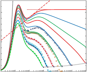
Figure 3. Solid lines: composite profiles of  $\langle uu\rangle ^+$ for
  $Re_{\tau } = 1000$ (green), 1995 (blue), 5186 (red), 20 250 (green), 98 190 (blue),
  $10^6$ (red),
  $10^7$ (green),
  $10^9$ (blue),
  $\infty$ (red). - - -, DNS profiles 5 (green), 4 (blue) and 1 (red) of table 1. Symbols:
  $\vartriangle \vartriangle \vartriangle$, NSTAP Superpipe profiles of Hultmark et al. (Reference Hultmark, Vallikivi, Bailey and Smits2012) at
  $Re_{\tau } = 1985$, 5411, 20 250 and 98 187;
  $\square$, ZPG TBL profile of Sillero et al. (Reference Sillero, Jiménez and Moser2013) for
  $Re_{\tau }= 1989$ (blue) and of Samie et al. (Reference Samie, Marusic, Hutchins, Fu, Fan, Hultmark and Smits2018) for
  $Re_{\tau } = 14\,500$ (orange). Note that TBL profiles have not been used for the construction of the composite expansion and are shown for comparison only. Long grey dashes (red for
  $Re_{\tau } = \infty$), wall log laws (2.5) for the
  $11\ Re_{\tau }$; short grey dashes (red for
  $Re_{\tau } = \infty$), corresponding overlap log laws (2.9) with
  $\circ$ marking their ‘end points’ at
  $y^+ = Re_{\tau }$;
  $\blacklozenge$, intersections of wall and overlap log laws at
  $y^+_\times$ (2.7); — (grey), fit (3.3) of
  $\langle uu\rangle ^+_{{CL}}$, with
  $\bullet$ marking the fit at the
  $Re_{\tau }$ values of the profiles shown;
  $\cdots$, leading term
  $0.25(y^+)^2$ of the Taylor expansion about the wall;
  $- \cdot -$, logarithmic slope of
  $-1.26$.
To actually form such an outer peak, the wall asymptote (2.5) has to cross over to a decay law at some  $y^+_\times$. This cross-over location
  $y^+_\times$ and the decay law beyond
  $y^+_\times$ could in principle be extracted from DNS data in a manner similar to the determination of
  $\langle uu\rangle ^+_{{wall}}$. Due to the complexity of the expansion and the limitations of the DNS data, this has not been possible. A first indication on the value of
  $y^+_\times$ comes from figure 1, which shows that the channel DNS closely follows the wall log law (2.5) up to
  $y^+\approx 200$, implying that
  $y^+_\times$ must be larger than 200.
Turning to a straight fit of  $y^+_\times$, all the data between
  $Re_{\tau } = 10^3$ and
  $10^5$ are seen in figure 3 to be compatible with
  $y^+_\times$ equal to a simple constant
 \begin{equation} y^+_\times{=} 470\quad \text{and}\quad \langle uu\rangle^+_\times{\equiv} \langle uu\rangle^+_{{wall}}(y^+_\times) = 10.48 - 42.0 Re_{\tau}^{{-}1/4}, \end{equation}
with the corresponding  $\langle uu\rangle ^+_\times$ following from ((2.5), (2.6)). To guide the eye, the points
  $(y^+_\times, \langle uu\rangle ^+_\times )$ are marked by
  $\blacklozenge$ for the profiles of figure 3. It is important to note here, that
  $\langle uu\rangle ^+_\times$ is not the outer maximum nor
  $y^+_\times$ its location, but the intersection of the logarithmic asymptote (2.5) with the asymptotic logarithmic decay law of the overlap region. As the actual outer peak height and its location depend on the slopes of both asymptotes, and on the manner the corner between them is smoothed, its detailed discussion is postponed to the short § 4, after the complete composite expansion is established in § 3.
The adoption of a constant  $y^+_\times$ for all
  $Re_{\tau }$ means that the inner expansion, which cannot end at a finite value of the inner coordinate, extends beyond the cross-over point
  $y^+_\times$ into the region of logarithmic decay, where it overlaps with the outer expansion. Hence, the complete inner expansion is obtained by adding a corner function (A5) to
  $\langle uu\rangle ^+_{{wall}}$ of (2.2)
 \begin{equation} \langle uu\rangle^+_{{in}} = \langle uu\rangle^+_{{wall}} + \mathcal{C}(y^+; y^+_\times, \Delta S, 2), \end{equation}
and its limit for  $y^+ \gg y^+_\times \gg 1$ yields the asymptotic logarithmic overlap layer, i.e. the common part of inner and outer expansions
 \begin{align} \langle uu\rangle^+_{{cp}} \equiv \langle uu\rangle^+_{{in}}(y^+{\gg} y^+_\times{\gg} 1) &= S_{{cp}}[\ln y^+{-} \ln y^+_\times ] + \langle uu\rangle^+_\times{+} \mathrm{HOT} \nonumber\\ \mathrm{with}\quad S_{{cp}} &= S_{{wall}} + \Delta S. \end{align}
 The logarithmic slope  $S_{{cp}}$ of the overlap log law (2.9) must be determined by matching to the outer expansion in § 3. At this point it can only be said that
  $S_{{cp}}$ must be negative to form an outer peak at large
  $Re_{\tau }$. Furthermore, it must go to zero at infinite
  $Re_{\tau }$, as shown in figure 3, because
  $\langle uu\rangle ^+$ near the wall has been shown to remain finite for all
  $Re_{\tau }$. This implies that
  $\Delta S$ is of the form
  $\Delta S = -0.85 + \Delta S'$, with
  $\Delta S'$ vanishing for
  $Re_{\tau }\to \infty$, to compensate the
  ${O}(1)$ contribution to
  $S_{{wall}}$ in (2.6).
3. The outer and composite expansions of $\langle uu\rangle ^+$

Moving on to the outer expansion, it is written as a logarithmic part matching the common part (2.9) for small  $Y$ and satisfying the symmetry condition on the centreline
  $Y=1$, plus a wake part
  $\mathcal {W}(Y)$, which goes to zero for
  $Y\to 0$
 \begin{equation} \langle uu\rangle^+_{{out}} = S_{{out}}\ln\left[Re_{\tau} Y \left(1 - \frac{Y}{2}\right)\right] - S_{{out}}\ln y^+_\times{+} \langle uu\rangle^+_\times{+} \mathcal{W}(Y) + \mathrm{HOT.} \end{equation}
The matching of outer and inner expansions furthermore requires  $S_{{out}}$ to be identical to
  $S_{{cp}}$ in (2.9).
To obtain the logarithmic slope  $S_{{out}} = S_{{cp}}$, the outer expansion (3.1) is evaluated at
  $Y=1$ and identified with the fit (3.3) of centreline stress
 \begin{align} \langle uu\rangle^+_{{CL}} &= S_{{out}}\ln\left(\frac{Re_{\tau}}2\right) - S_{{out}}\ln y^+_\times{+} \langle uu\rangle^+_\times{+} \mathcal{W}(1) \end{align}
 \begin{align} &= 0.55 + [0.1007 + 33Re_{\tau}^{{-}1/4}]^{{-}1} . \end{align}
As seen in figure 3, this fit reproduces the channel and Superpipe centreline data up to  $Re_{\tau } = 10^5$. At higher
  $Re_{\tau }, \langle uu\rangle ^+_{{CL}}$ increases to the infinite Reynolds number limit of
  $\langle uu\rangle ^+_{\times } = 10.48$, such that
  $\langle uu\rangle ^+_{{out}}$ becomes a simple constant throughout the channel or pipe. Note that the fit (3.3), which relies strongly on the outer Superpipe data of Hultmark et al. (Reference Hultmark, Vallikivi, Bailey and Smits2012), implies that differences are relatively minor between the outer expansions for pipe and channel (see comments in § 5).
What is still missing for the determination of the outer logarithmic slope  $S_{{out}}$ is the wake function
  $\mathcal {W}(Y)$. The fit with the requisite symmetry properties
 \begin{equation} \mathcal{W}(Y) = S_{{out}}\ln\left[\frac{1}4 + \frac{3}4(1-Y)^2\right], \end{equation}
is again developed from both channel DNS and Superpipe NSTAP data, while ZPG TBLs obviously require a different  $\mathcal {W}(Y)$. However, it appears from figure 3, that the TBL overlap log law remains close to (2.9) developed for channel and pipe.
Equation (3.4), together with (3.2) and (3.3), finally allows one to determine  $S_{{out}} = S_{{cp}}$ in (2.9). The resulting logarithmic slope is found to scale as
 \begin{equation} S_{{out}} = \sigma \ln^2Re_{\tau} Re_{\tau}^{{-}1/4}, \end{equation}
with  $\sigma$ a weak function of
  $Re_{\tau }$, varying between −0.19 and −0.15 in the interval
  $Re_{\tau } \in [10^3, 10^{10}]$. While the
  $Re_{\tau }^{-1/4}$ dependence is directly related to the scaling of
  $\langle uu\rangle ^+_{{in}}$, obtained without model assumptions, the factor
  $\ln ^2Re_{\tau }$ in (3.5) may depend on the details of how
  $S_{{out}}$ has been determined. However, as long as
  $\langle uu\rangle ^+_\times$ remains finite,
  $S_{{out}}$ must go to zero for
  $Re_{\tau } \to \infty$.
With the determination of  $S_{{out}}$, the composite expansion
 \begin{equation} \langle uu\rangle^+_{{comp}} = \langle uu\rangle^+_{{in}} + \langle uu\rangle^+_{{out}} - \langle uu\rangle^+_{{cp}}, \end{equation}
is complete up to  ${O}(Re_{\tau }^{-1/4})$. This final result is compared in figure 4 with the DNS data of table 1, and the differences between composite expansion and DNS are seen to be at most
  $1.5\,\%$ of the inner peak height (2.4). It is also noted that, in the region
  $0 \leq y^+ \lessapprox 10^2$, the difference between DNS and composite expansion is principally due to an imperfect ‘hump’ function (A4). However, no improvement is pursued here, as the deviations from DNS are barely larger than the line thickness in figure 1 and no additional insight would be gained from a more complex
  $\mathcal {H}$.


The composite expansion (3.6) allows a unified comparison with complete  $\langle uu\rangle ^+$ profiles of different origins, as well as an extrapolation of
  $\langle uu\rangle ^+$ to truly large
  $Re_{\tau }$. Figure 3 shows the close correspondence, over the entire
  $Re_{\tau }$ range of
  $10^3$ to
  $10^5$, between composite profiles and both DNS and several more recent high Reynolds number laboratory data. Only the Superpipe data of Hultmark et al. (Reference Hultmark, Vallikivi, Bailey and Smits2012) are seen to progressively fall below the composite expansion close to the wall, which is also reflected in the low inner peak heights for the Superpipe in figure 2. An explanation for these discrepancies is proposed in Appendix B.
Figure 3 also shows the asymptotic ‘skeleton’ of the composite expansion: the fan of logarithmic asymptotes (2.5) of  $\langle uu\rangle ^+_{{wall}}$ (2.2) and the corresponding asymptotic overlap log laws (2.9), together with their intersections (2.7), marked by
  $\blacklozenge$. The considerable difference, at the lower Reynolds numbers, between this asymptotic logarithmic ‘skeleton’ and the composite expansion, is already noted here. Similarly, the data are seen to closely approach the overlap log law (2.9) – the short-dashed grey lines between
  $\blacklozenge$ and
  $\circ$ in figure 3 – only beyond a
  $Re_{\tau }$ of approximately
  $10^5$. Below this
  $Re_{\tau }$, the wake region is reached before the condition
  $y^+\gg y^+_\times$ is satisfied. See also the comments in the concluding § 5 and the comparison with the patched asymptotic expansion of Marusic & Kunkel (Reference Marusic and Kunkel2003) in figure 3 of the supplementary material.
4. The outer peak
The scaling of the outer peak  $\langle uu\rangle ^+_{{OP}}$ and its location
  $y^+_{{OP}}$ have given and still give rise to extended debates, because they are not yet accessible to DNS and in experiments are typically seen at a wall distance where probe corrections are often an important issue. Probably the first, clean characterization of this peak has been provided by Samie et al. (Reference Samie, Marusic, Hutchins, Fu, Fan, Hultmark and Smits2018) for the ZPG TBL at
  $Re_{\tau }$ values up to 20’000. The Reynolds number dependence of the outer peak, observed by Samie et al. (Reference Samie, Marusic, Hutchins, Fu, Fan, Hultmark and Smits2018), appears to clash with the choice of a constant
  $y^+_\times$ in (2.7). A close look at figure 3 shows, however, that the location
  $y^+_{{OP}}$ of the actual outer peak depends strongly on the slopes of the wall and overlap log laws (2.5) and (2.9), as well as on how the transition between the two is fitted. This sensitivity to fitting details is comparable to the sensitivity to measurement errors in experiments (see also Appendix B).
The evolutions of the outer peak height  $\langle uu\rangle ^+_{{OP}}$ and location
  $y^+_{{OP}}$ with
  $Re_{\tau }$, obtained from the present composite expansion (3.6), are shown in figure 5;
  $\langle uu\rangle ^+_{{OP}}$, which is always below
  $\langle uu\rangle ^+_\times$ (2.7), is seen in panel (a) to be fully consistent with other experimental data, as well as with the outer peak correlations
  $2.82+0.42\ln Re _{\tau }$ and
  $0.33+0.63\ln Re _{\tau }$ of Pullin et al. (Reference Pullin, Inoue and Saito2013), up to
  $Re_{\tau }$ values well above
  $10^6$.

Figure 5. (a) Outer peak height  $\langle uu\rangle ^+_{{OP}}$ vs
  $Re_{\tau }$. Symbols as in figure 2, except for: green
  $\blacklozenge$, pipe data point of Morrison et al. (Reference Morrison, McKeon, Jiang and Smits2004); red
  $\bullet$, outer peak height of full composite expansion (3.6) at selected
  $Re_{\tau }$ values; red —,
  $\langle uu\rangle ^+_\times$ of (2.7); black - - - and
  $- \cdot - \cdot -$, outer peak correlations
  $2.82+0.42\ln Re _{\tau }$ and
  $0.33+0.63\ln Re _{\tau }$ of Pullin, Inoue & Saito (Reference Pullin, Inoue and Saito2013). (b) Corresponding outer peak locations
  $y^+_{{OP}}$. Symbols as in panel (a), except for: red —,
  $y^+_\times = 470$; blue - - -, correlation of Hultmark et al. (Reference Hultmark, Vallikivi, Bailey and Smits2012); red
  $\cdots$, fit
  $1200 - 1900Re_{\tau }^{-0.06}$; yellow
  $- \cdot - \cdot -$, correlation
  $32.66\ Re_{\tau }^{0.27}$ of Samie et al. (Reference Samie, Marusic, Hutchins, Fu, Fan, Hultmark and Smits2018, (3.3b)) for the intersection of tangents outside of
  $y^+_{{OP}}$.
Panel (b) shows the location  $y^+_{{OP}}$ vs
  $Re_{\tau }$. In this panel, the uncertainty of the experimental points is large and could be as high as 100 % at the lower
  $Re_{\tau }$ values. Up to
  $Re_{\tau }=10^5$ the outer peak locations for both the data and the present composite expansion are seen to be compatible with the correlation
  $\propto Re_{\tau }^{0.67}$ of Hultmark et al. (Reference Hultmark, Vallikivi, Bailey and Smits2012). Samie et al. (Reference Samie, Marusic, Hutchins, Fu, Fan, Hultmark and Smits2018, (3.3b)), on the other hand, give a correlation of
  $32.66Re_{\tau }^{0.27}$ for the intersection of two logarithmic tangents to the data, which is located outside of the outer peak, and provides an upper bound on
  $y^+_{{OP}}$. Together with the outer peak location of the present composite expansion, which is well fitted by the ad hoc correlation
  $y^+_{{OP}} = 1200 - 1900Re_{\tau }^{-0.06}$, the outer peak is firmly placed in the inner asymptotic region, meaning that, in terms of the usual intermediate or overlap variable
  $\eta =y^+/Re_{\tau }^{1/2}$, the outer peak approaches
  $\eta = 0$ in the limit of
  $Re_{\tau } \to \infty$.
5. Discussion and outlook
In conclusion, the first complete composite profile of  $\langle uu\rangle ^+$, based on the inner asymptotic sequence
  $\{1, Re_{\tau }^{-1/4},\ldots \}$ proposed by CS2021, provides a rather satisfactory description of DNS and experimental
  $\langle uu\rangle ^+$ profiles for Reynolds numbers between
  $10^3$ and
  $10^5$, as seen in figure 3. What is curious, however, is that CS2021 and Smits et al. (Reference Smits, Hultmark, Lee, Pirozzoli and Wu2021) fully agree on the proportionality between the inner peak height
  $\langle uu\rangle ^+_{{IP}}$ and the coefficient of
  $(y^+)^2$ in the Taylor expansion of
  $\langle uu\rangle ^+$ about the wall and even on the value of their ratio, while completely disagreeing on the Reynolds number scaling of the two quantities. Furthermore, the
  $Re_{\tau }^{-1/4}$ scale, or any other scale, apart from
  $Re_{\tau }^{-1}$, does not appear naturally in the Reynolds stress transport equation for
  $\langle uu\rangle ^+$. What is particularly intriguing is that the exact production term for channel flow,
  $\mathcal{P}^+ = (dU^+/dy^+)(1 - dU^+/dy^+ - y^+/Re_{\tau})$, does not vary as
  $Re_{\tau }^{-1/4}$, but has an inner asymptotic expansion of the form
  $\mathcal {P}^+_0(y^+) + Re_{\tau }^{-1}\mathcal {P}^+_1(y^+) + \cdots$ (see Monkewitz Reference Monkewitz2021).
If the correct expansion parameter was indeed  $(1/Re_{\tau })$, clearly more than two terms would be required in the inner expansion of
  $\langle uu\rangle ^+$ for a good approximation at the Reynolds numbers of the DNS data in table 1, that is
 \begin{equation} \langle uu\rangle^+ \approxeq f(y^+) + g(y^+)Re_{\tau}^{{-}1/4} \approxeq f(y^+) + \sum_{n=1}^{N} h_n(y^+)Re_{\tau}^{{-}n}. \end{equation}
 This is illustrated for the inner peak height in figure 6(a), which is figure 2 replotted against  $Re_{\tau }^{-1}$, with the addition of the relatively simple fit
 \begin{align} \langle uu\rangle^+_{{IP}} = 7.6 + 1.9 \exp\left(\frac{-1300}{Re_{\tau}}\right) + \exp\left(\frac{-15000}{Re_{\tau}}\right) = 10.5 - \frac{1.75\,10^4}{Re_{\tau}} + {O}(Re_{\tau}^{{-}2}), \end{align}
and its two-term Taylor expansion. This fit is seen to describe the Reynolds number dependence of all the  $\langle uu\rangle ^+_{{IP}}$ data included in figure 2 as well as the other correlations, and its two-term Taylor expansion provides an excellent fit for
  $Re_{\tau } \gtrapprox 2.10^4$. Figure 6(b) shows that the fit (5.2) divided by 46 is again an excellent match for the coefficient of
  $(y^+)^2$ in the Taylor expansion about the wall. However, one immediately notices that this coefficient only reaches 0.228 instead of the 0.25 inferred by CS2021. This discrepancy may well be due to the simplifying assumptions of CS2021. Actually, the ratio between the production at
  $y^+_{{IP}} \approxeq 15$ and the turbulent transport at the wall in the DNS 1 of table 1 is 1.12, tantalizingly close to the ratio
  $0.25/ 0.228 = 1.10$. Finally, the fact that the first two terms of the Taylor expansion in (5.2) require a
  $Re_{\tau }$ in excess of
  $10^4$ to provide a good approximation of the full exponential fit is reminiscent of the behaviour of the indicator function
  $\varXi ^+ = y^+(\textrm {d}U^+/{\textrm {d} y}^+)$ in figure 12 of Monkewitz (Reference Monkewitz2021), which starts to reach the correct log-law plateau only for Reynolds numbers around
  $10^5$.

Figure 6. (a) Inner peak height  $\langle uu\rangle ^+_{{IP}}$ vs
  $(1/Re_{\tau })$ with same data as in figure 2. Lines: (red) —, (2.4); (wide grey) —, (5.2); (grey)
  $\cdots$, two-term Taylor expansion of ‘grey’ fit;
  $\leftarrow$, lower end of the range of the atmospheric inner peak data of Metzger & Klewicki (Reference Metzger and Klewicki2001) at
  $Re_{\tau } \approxeq 8.10^5$. (b) Coefficient of
  $(y^+)^2$ in the Taylor expansion of
  $\langle uu\rangle ^+$ about the wall: (red)
  $\bullet$, DNS data 1, 4 and 5 of table 1; (red) —, (2.3); (wide grey) —, (5.2) divided by 46; (grey)
  $\cdots$, two-term Taylor expansion
  $0.228 - 380/Re_{\tau }$ of ‘grey’ fit.
Beyond these speculations on scaling, which require more thought, the features of the  $\langle uu\rangle ^+$ profiles, shown in figure 3, call for the following comments and conclusions:
(i) The analysis of the channel DNS profiles of table 1 in § 2 has demonstrated, that the structure of the inner asymptotic expansion of
$\langle uu\rangle ^+$ does not change between the wall and $y^+\approx 200$, and supports the somewhat complex argument of CS2021 that $\langle uu\rangle ^+$ remains finite in the limit of infinite Reynolds number. It has furthermore demonstrated that the coefficient of $(y^+)^2$ in the Taylor expansion of $\langle uu\rangle ^+$ about the wall and the inner peak height $\langle uu\rangle ^+_{{IP}}$ at $y^+\approx 15$ are proportional, or nearly so, which has been fully confirmed by the data analyses of Hultmark & Smits (Reference Hultmark and Smits2021) and Smits et al. (Reference Smits, Hultmark, Lee, Pirozzoli and Wu2021).(ii) The detailed analysis of the transport equation for
$\langle uu\rangle ^+$ in § 2 has shown that the unlimited growth of $\langle uu\rangle ^+_{{IP}}$ with $\ln Re_{\tau }$, predicted by the attached eddy model (Marusic & Monty Reference Marusic and Monty2019) is very unlikely. The possibility of an unlimited growth of the outer peak with $Re_{\tau }$ appears equally unlikely, considering that the cross-over location $y^+_\times$ from the wall log law (2.5) to the overlap log law not only scales on inner units, but remains constant over the $Re_{\tau }$ range where laboratory data are available, as seen in figure 3.(iii) As discussed in § 4, the present composite profiles in figure 3 also match, within the considerable uncertainty, the height and location of distinct outer peaks reported in the literature, with the notable exception of some NSTAP data discussed in Appendix B.
(iv) With both inner and outer peaks of
$\langle uu\rangle ^+$ finite, a simple geometric argument, already brought up by Monkewitz & Nagib (Reference Monkewitz and Nagib2015), rules out the Reynolds-independent slope of the overlap log law in the attached eddy model (see figure 3 in § 2 of the supplementary material). Due to its relatively simple structure, it appears nevertheless useful, if parameters are adapted to the Reynolds number range under consideration.(v) The switch over from the wall log law to the asymptotic overlap log law at a fixed value of
$y^+_\times \approxeq 470$ is reminiscent of the change of logarithmic slope from $1/0.398$ to $1/0.42$ at $y^+ = 624$, found by Monkewitz (Reference Monkewitz2021) in the mean velocity profile and tentatively interpreted as an opposite wall effect. A connection between the two observations is conceivable, but the mechanism remains to be elucidated.(vi) Also open is the question whether the
$\langle uu\rangle ^+$ composite expansion developed here is universal or not, excluding of course the wake region in ZPG TBLs. For the near-wall region in figure 1, the present expansion relies entirely on channel DNS, while at the higher $Re_{\tau }$, the outer part of the Superpipe profiles of Hultmark et al. (Reference Hultmark, Vallikivi, Bailey and Smits2012) has helped guide the expansion. The close correspondence in figure 3 between the channel DNS and Superpipe profiles for $Re_{\tau }$ of 1985 and 5411 suggests that the differences between channel and pipe are small. It would, however, be surprising if there were no differences at all, at least in the outer $\langle uu\rangle ^+$ expansion, as there are strong indications (Monkewitz Reference Monkewitz2021) that the outer mean velocity expansions, in particular the Kármán ‘constants’, are different for channel and pipe. In ZPG TBLs, finally, $\langle uu\rangle ^+$ also appears to remain close to channel and pipe, up to and including the overlap layer. However, the present asymptotic expansion underestimates the inner peak heights in the atmospheric data of Metzger & Klewicki (Reference Metzger and Klewicki2001), indicated in figure 6(a) by an arrow, but no attempt has been made here to untangle the possible reasons.(vii) Finally, it must be reiterated that determining the slopes of log laws, which are inherently asymptotic laws, by fitting tangents to finite Reynolds number data is hazardous. As illustrated in figure 3, only at the highest NSTAP
$Re_{\tau }$ of around $10^5$ does the overlap log law start to go through the data! This is the same conclusion as the one reached by Monkewitz (Reference Monkewitz2021, figure 12) and Spalart & Abe (Reference Spalart and Abe2021, see their extrapolation in figure 3b), who found that the mean velocity indicator function $y^+(\mathrm {d}U^+/\mathrm {d} y^+)$ starts to reach the correct log-law plateau only beyond a $Re_{\tau }$ of around $10^5$. Up to such high $Re_{\tau }$, the development of proper asymptotic expansions is indispensable.


Supplementary material
Supplementary material are available at https://doi.org/10.1017/jfm.2021.924.
Acknowledgements
I am grateful to K. ‘Sreeni’ Sreenivasan, H. Nagib, X. Chen and an anonymous reviewer for their helpful comments and encouragement. Thanks also to M. Hultmark for the stimulating discussion on Appendix B.
Declaration of interest
The author reports no conflict of interest.
Appendix A. The fit for the near-wall $\langle uu\rangle ^+$ profile and other fits

Inspired by the methodology of Musker (Reference Musker1979) for the mean velocity fit, the  ${O}(1)$ part of the inner (near-wall)
  $\langle uu\rangle ^+$ Reynolds stress profile is approximated analytically by the integral of
  $\textrm {d} \mathcal {M}_2/\textrm {d} y^+ = 2 p_0 y^+ [p_1 + p_2(y^+)^2][p_1 + p_3(y^+)^2 + (y^+)^4]^{-1}$, where the subscript ‘2’ indicates that the leading term of the Taylor expansion of
  $\mathcal {M}_2$ around
  $y^+=0$ is
  $\propto (y^+)^2$. The result of the integration is
 \begin{align} \mathcal{M}_2(y^+; p_0, p_1, p_2, p_3) &= \frac{p_0 (2p_1-p_2p_3)}{\sqrt{4p_1-p_3^2}}\left\{\arctan \frac{p_3+2(y^+)^2}{\sqrt{4p_1-p_3^2}} - \arctan \frac{p_3}{\sqrt{4p_1-p_3^2}}\right\} \nonumber\\ &\quad +\frac{p_0 p_2}{2} \ln\left[1 + \frac{p_3 (y^+)^2}{p_1} + \frac{(y^+)^4}{p_1}\right] , \end{align}
with the parameters  $p_0 \cdots p_3$ determined by the boundary conditions. For large
  $y^+, \mathcal {M}_2$ asymptotes to the log law
 \begin{align} \mathcal{M}_2(y^+{\gg} 1) = \frac{p_0 p_2}{2}\{4 \ln(y^+)-\ln(p_1)\} + \frac{p_0}{\sqrt{4p_1-p_3^2}}\left\{\frac{\rm \pi}{2} - \arctan \frac{p_3}{\sqrt{4p_1-p_3^2}}\right\}, \end{align}
and near the wall it has the Taylor expansion
 \begin{equation} \mathcal{M}_2(y^+\to 0) = p_0 (y^+)^2 + \frac{p_0 (p_2 - 2p_3)}{2 p_1}(y^+)^4 + \cdots . \end{equation}
 Like the original mean velocity Musker profile, the profile (A1) misses a ‘hump’ centred around  $y^+ ={O}(10)$. As in Monkewitz (Reference Monkewitz2021), it is modelled by the ‘hump’ function of Nagib & Chauhan (Reference Nagib and Chauhan2008)
 \begin{equation} \mathcal{H}(y^+; h_1, h_2, h_3) = h_1 \exp[- h_2 \ln^2(y^+{/}h_3)]. \end{equation}
 Finally, the smooth transition between two logarithmic laws with different slopes in a variable  $\eta$ is fitted by the corner function
 \begin{equation} \mathcal{C}(\eta; \eta_c, c, m) = \frac{c}{m} \ln\left[1 + \left(\frac{\eta}{\eta_c}\right)^m\right] \rightarrow \left\{ \begin{array}{ll} 0 & \text{for }\eta\ll\eta_c \\ c[\ln\eta-\ln\eta_c] & \text{for } \eta\gg\eta_c \end{array} \right. \end{equation}
with the rounding of the corner at  $\eta _c$ governed by the parameter
  $m$.
$m$.
Appendix B. Survey of the effect of wall proximity on NSTAP measurements
The debate on whether near-wall statistics in turbulent wall-bounded flows are universal or not depends crucially on experimental data at high Reynolds numbers. Focussing on the streamwise Reynolds stress, the problem is exemplified by the discrepancies between measured inner peak heights  $\langle uu\rangle ^+_{{IP}}$ in figure 2. Of particular interest is the marked difference between the CICLoPE data of Fiorini (Reference Fiorini2017) and the Superpipe data of Hultmark et al. (Reference Hultmark, Vallikivi, Bailey and Smits2012), both corrected for spatial probe averaging. Since the corrections (shown in the figure for the CICLoPE data) are rather large and the probes very different (standard hot-wire vs NSTAP, described in Vallikivi & Smits Reference Vallikivi and Smits2014), it has not yet been possible to explain the origin of the discrepancy.
To advance the discussion, the NSTAP measurements in two different ZPG TBL facilities are compared, one in the Melbourne wind tunnel at atmospheric pressure by Samie et al. (Reference Samie, Marusic, Hutchins, Fu, Fan, Hultmark and Smits2018) and the other in the pressurized Princeton facility by Vallikivi et al. (Reference Vallikivi, Hultmark and Smits2015) (available from https://smits.princeton.edu). The comparison is shown in figure 7 and reveals a significant difference between the two  $\langle uu\rangle ^+$ data sets below a
  $y^+$ of the order of
  $10^2$. Looking for corresponding differences of operating parameters in the two set-ups, the physical wall distance of the sensing element is the most conspicuous. In the pressurized Princeton facility, a wall distance of
  $300\ \mathrm {\mu }$m corresponds to
  $y^+$ of 90 and more, indicated in figure 7 by vertical dashed lines for the three
  $Re_{\tau }$ values. In the Melbourne tunnel, the same
  $300\ \mathrm {\mu }$m correspond to
  $y^+ \leq 17$ for the similar
  $Re_{\tau }$ values of Samie et al. (Reference Samie, Marusic, Hutchins, Fu, Fan, Hultmark and Smits2018). Lacking any other credible candidates, an explanation based on the difference between length scales
  $\hat {\nu }/\hat {u}_\tau$ is proposed.

Figure 7. Comparison of NSTAP profiles of  $\langle uu\rangle ^+$ and
  $U^+$ in different ZPG TBL facilities. Solid lines:
  $\langle uu\rangle ^+$ of Samie et al. (Reference Samie, Marusic, Hutchins, Fu, Fan, Hultmark and Smits2018) at
  $Re_{\tau } = 10\ 000$ (blue), 14 500 (green) and 20 000 (red); vertical solid lines:
  $y^+$ locations corresponding to a wall distance of
  $300\ \mathrm {\mu }$m. Symbols:
  $\langle uu\rangle ^+$ of Vallikivi, Hultmark & Smits (Reference Vallikivi, Hultmark and Smits2015) at
  $Re_{\tau } = 8260$ (blue
  $\blacktriangle$), 14 700 (green
  $\blacklozenge$) and 25 000 (red
  $\bullet$) and corresponding
  $U^+$ profiles (open symbols); vertical dashed lines:
  $y^+$ locations corresponding to wall distance of
  $300\ \mathrm {\mu }$m.
  $\times$: local minimum and outer maximum of
  $\langle uu\rangle ^+$ from figure 43 of Fernholz & Finley (Reference Fernholz and Finley1996) for
  $Re_{\tau }\approxeq 18\ 000\ ({Re}_{\delta 2}=57\ 720$); - - -,
  $U^+$ profile of Sillero et al. (Reference Sillero, Jiménez and Moser2013) for
  $Re_{\tau } = 1989$; —,
  $(1/0.384)\ln Re_{\tau } + 4.17$.
The fact that the  $300\ \mathrm {\mu }$m wall distance, below which the discrepancies emerge, is much larger than the NSTAP sensing element, which is a ‘flat plate’ of roughly
  $0.1\ \mathrm {\mu }$m thickness and 1
 $\ \mathrm {\mu }$m chord, suggests that the ‘culprit’ may be the NSTAP silicon support structure, with overall dimensions of
  $4\times 2.1$ mm and a thickness increasing downstream to
  $0.5$ mm. The difference between the
  $\langle uu\rangle ^+$ of Samie et al. (Reference Samie, Marusic, Hutchins, Fu, Fan, Hultmark and Smits2018) and those of Vallikivi et al. (Reference Vallikivi, Hultmark and Smits2015) in figure 7 is seen to reach about one for
  $y^+$ in the range of 20–30. In the same region, the mean velocities of Vallikivi et al. (Reference Vallikivi, Hultmark and Smits2015) are clearly above the DNS profile of Sillero et al. (Reference Sillero, Jiménez and Moser2013), again with a difference of order unity, while those of Samie et al. (Reference Samie, Marusic, Hutchins, Fu, Fan, Hultmark and Smits2018), not shown in the figure for clarity, are slightly below the DNS. This behaviour suggests a blockage effect of the NSTAP probe body when the volume between the two wedge shaped silicon sensor supports is progressively closed off by the wall, leading at the sensor location to a mean flow acceleration at the expense of turbulence intensity.
For comparison, the deviation of the Superpipe NSTAP data of Hultmark et al. (Reference Hultmark, Vallikivi, Bailey and Smits2012) from the composite profile (3.6) is shown in figure 8 and the similarity with the deviations between the Princeton and Melbourne ZPG TBL data, shown in figure 7, is obvious. This supports the idea that the  $\langle uu\rangle ^+$ profiles in pipes, ZPG TBLs and most probably channels are very similar, possibly even identical, well into the overlap region beyond
  $y^+_\times$ (
 $\blacklozenge$ in figure 3). However, it should be noted that the NSTAP pipe data in figure 8 are being compared with a composite expansion developed mainly on lower Reynolds number channel DNS and that the suspected origin of the discrepancy – near-wall blockage by the NSTAP silicon probe support, likely also dependent on its angle of attack – will have to be tested experimentally.

Figure 8. Difference between the composite expansion (3.6) and eight Superpipe NSTAP profiles of  $\langle uu\rangle ^+$ (Hultmark et al. Reference Hultmark, Vallikivi, Bailey and Smits2012), from
  $Re_{\tau }=98\,187$ to 1985 (available from https://smits.princeton.edu); colour sequence red, pink, violet, light blue, light green, dark green, orange, brown. Vertical - - -,
  $y^+$ values corresponding to 300
 $\ \mathrm {\mu }$m wall distance for each
  $Re_{\tau }$.


 Open access