


1. INTRODUCTION
The Tibetan Plateau (TP), known as the roof of the world or Third Pole, contains the largest concentration of glaciers and icefields outside the polar regions (Yao and others, Reference Yao, Ren and Xu2008). Meltwater from these feeds the headwaters of many prominent Asian rivers (e.g. the Yellow, Yangtze, Mekong, Salween, Brahmaputra, Ganges and Indus) (Immerzeel and others, Reference Immerzeel, van Beek and Bierkens2010), and are a key component of the cryospheric system (Li and others, Reference Li2008). Glaciers are important climate indicators because their extent and thickness adjust in response to climate change (Oerlemans, Reference Oerlemans1994; Yao and others, Reference Yao2012). With a warming climate, many mountain glaciers have shrunk progressively in mass and extent during the past few decades (IPCC, 2013). However, slight mass gains or balanced mass budgets have been evident for parts of the central Karakoram, eastern Pamir and the western TP in recent years (Gardelle and others, Reference Gardelle, Berthier and Arnaud2012b, Reference Gardelle, Berthier, Arnaud and Kääb2013; Yao and others, Reference Yao2012; Neckel and others, Reference Neckel, Kropáček, Bolch and Hochschild2014; Bao and others, Reference Bao, Liu, Wei and Guo2015; Kääb and others, Reference Kääb, Treichler, Nuth and Berthier2015; Ke and others, Reference Ke, Ding and Song2015). The relationships between glacier mass balance and climate change, water supply and the risk of glacier-related disasters, are the subject of much current research.
It is difficult to carry out in situ observations on the TP due to its rugged terrain and the great labor and logistical costs. Only 15 glaciers have decades of traditional mass-balance measurements (Yao and others, Reference Yao2012). By comparing elevation data from more than two points in time, glacier height and volume changes can be determined and hence glacier mass balance, after consideration of ice/firn/snow densities (Bolch and others, Reference Bolch, Pieczonka and Benn2011; Kääb and others, Reference Kääb, Berthier, Nuth, Gardelle and Arnaud2012; Gardelle and others, Reference Gardelle, Berthier, Arnaud and Kääb2013; Pieczonka and others, Reference Pieczonka, Bolch, Wei and Liu2013; Shangguan and others, Reference Shangguan2014; Paul and others, Reference Paul2015; Brun and others, Reference Brun, Berthier, Wagnon, Kääb and Treichler2017; Zhou and others, Reference Zhou, Li, Li, Zhao and Ding2018).
Glaciers in south-eastern Tibet are classified as temperate (maritime) type and are influenced by the South Asian monsoon (Li and others, Reference Li, Zheng and Yang1986; Shi and Liu, Reference Shi and Liu2000). Based on inventories from maps and remote sensing, or field measurements, a substantial reduction in glacier area and length has been recorded in this region from 1980 to 2013, as well as a glacier mass deficit from 2005 to 2009 (Yang and others, Reference Yang2008, Reference Yang2010; Yao and others, Reference Yao2012; Li and others, Reference Li, Yang and Ji2014). Most previous studies used satellite laser altimetry or stereo photogrammetry to calculate the glacier height changes that determined pronounced negative glacier mass balances in the region (Gardelle and others, Reference Gardelle, Berthier, Arnaud and Kääb2013; Gardner and others, Reference Gardner2013; Neckel and others, Reference Neckel, Kropáček, Bolch and Hochschild2014; Kääb and others, Reference Kääb, Treichler, Nuth and Berthier2015), although the results did differ slightly from each other. Laser altimetry from the ICESat (Ice, Cloud and Land Elevation Satellite) showed geodetic glacier-elevation difference trends in south-eastern Tibet during 2003–2008 of −1.34 ± 0.29 m a−1 (Kääb and others, Reference Kääb, Treichler, Nuth and Berthier2015), −0.81 ± 0.32 m a−1 (Neckel and others, Reference Neckel, Kropáček, Bolch and Hochschild2014) and −0.30 ± 0.13 m a−1 (Gardner and others, Reference Gardner2013), respectively. The large orbital gaps in ICESat footprint data mean spatial details cannot be mapped at a fine scale. A comparison between ASTER images found a mean glacier mass balance of −0.62 ± 0.23 m w.e. a−1 in Nyainqentanglha from 2000 to 2016 (Brun and others, Reference Brun, Berthier, Wagnon, Kääb and Treichler2017).
While stereo photogrammetry provides high resolution details on glacier height changes, it can be limited by image saturation, particularly at high elevations. Furthermore, the lack of local mass-balance measurements prevents analysis of glacier responses to climate change in the central Nyainqentanglha Range (CNR). Based on the Shuttle Radar Topography Mission (SRTM) and an interferometrically derived TanDEM-X elevation model, glaciers were determined to have experienced strong surface lowering in the CNR, at an average rate of −0.83 ± 0.57 m a−1 from 2000 to 2014 (Neckel and others, Reference Neckel, Loibl and Rankl2017). While this pronounced surface-lowering value came from five debris-covered valley glaciers which are located in the east of the study area, it does not represent large scale glacier response to climate warming. For the climate background, most meteorological stations, located in inhabited river valleys, are far from the glacierized high-mountain regions so their records cannot be used directly as climate background for them. Even in the same climate environment, glacier responses may differ due to local parameters, such as aspect, topography and debris cover (Kääb, Reference Kääb2005; Scherler and others, Reference Scherler, Bookhagen and Strecker2011; Neckel and others, Reference Neckel, Loibl and Rankl2017).
This study calculates geodetic glacier mass balances for a large number of glaciers in the CNR. Most glaciers have been mapped from aerial photographs taken in October 1980 and subsequently by SAR Interferometry (InSAR) in February 2000 (during the SRTM), resulting in a digital elevation model (DEM). Single-pass X-band InSAR from TerraSAR-X and TanDEM-X digital elevation measurements provided the basis for another map (Krieger and others, Reference Krieger2007). Bistatic Differential Synthetic Aperture Radar Interferometry (DInSAR) and common DEM differencing were used to estimate the geodetic glacier mass balance in different sub-regions of the CNR between 1968 and 2013.
2. STUDY REGION
The CNR (30°9′– 30°53′ N, 94°0′– 95°30′ E) lies in south-eastern Tibet, north of Linzhi County, east of Jiali County and west of Bomi County, and extends ~130 km from west to east. South of this region is the Yigong Tsangpo River, a tributary of the Purlung Tsangpo River and a secondary tributary of the Yarlung Tsangpo River (Fig. 1). The elevation differences between mountain peaks and valley bottoms often reach 3000–3500 m. The rugged topography with steep valleys and slopes results from the interplay of a still ongoing tectonic uplift and erosion (Li and others, Reference Li, Zheng and Yang1986). High precipitation amounts during the summer monsoon season (May to September) are the main reason for the intense erosion. The CNR is characterized by a strong climatic influence of the South Asian monsoon entering through the Yarlung Tsangpo valley (Loibl and others, Reference Loibl, Lehmkuhl and Grießinger2014). More than 80% of annual precipitation falls from June to September, while winter months are characterized by cold and dry conditions (Molnar and others, Reference Molnar, Boos and Battisti2010). According to the climatic classification of local meteorological station data, the CNR marks a transition zone between warm-wet subtropical and cold-dry plateau conditions (Leber and others, Reference Leber, Holawe and Häusler1995). Previous studies showed that average annual precipitation in most high-elevation areas in the CNR exceeds 2000 mm (Shi and others, Reference Shi, Huang and Ren1988). Farther north, the east–west orientation of the mountain range acts as a topographic barriers that produces heavy orographic rainfalls (Böhner, Reference Böhner2006; Maussion and others, Reference Maussion2014). This results in a distinct precipitation gradient that decreases from south to north (Shi and others, Reference Shi, Huang and Ren1988).
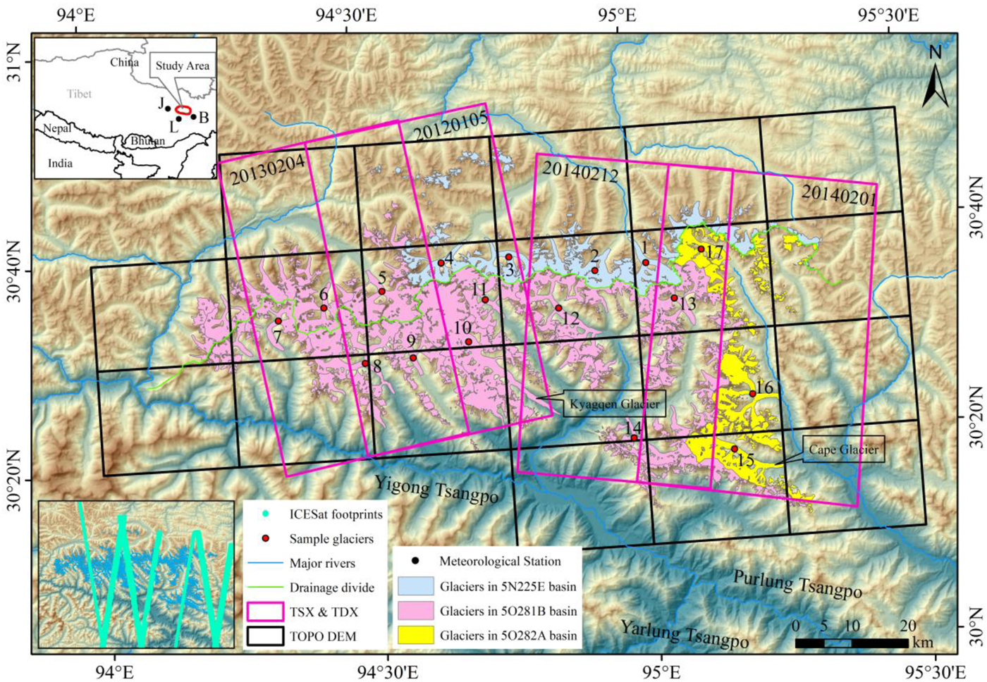
Fig. 1. Study area and distribution of 2016 glacier outlines in different drainage basins, and the location of the meteorological stations (J: Jiali station, L: Linzhi station, B: Bomi station). TOPO DEMs, TSX/TDX acquisitions and ICESat footprints. Numbers indicate specific sample glaciers chosen for analysis. The background map is SRTM DEM.
The first Chinese Glacier Inventory (CGI) determined that glaciers covered 2537.7 km2 of our study region, with an estimated total volume of 454.2 km3 in 1968 (Pu, Reference Pu2001; Mi and others, Reference Mi2002). At this time, ~8% of the glacier area was covered by debris. Three glaciers in the CNR are larger than 100 km2, the Xiaqu (CGI code: 5O281B0702), Kyagqen (CGI code: 5O281B0729) and Nalong (CGI code: 5O281B0768). The Kyagqen, on the south slope of the CNR, 35.3 km long and 206.7 km2, with a terminus at 2900 m a.s.l., is the largest of these (Li and others, Reference Li, Zheng and Yang1986). Above 4000 m a.s.l. it has a broad basin in which several ice streams converge to form a large accumulation zone. Below this, the glacier enters a narrow ice-filled valley where its velocity increases, and the tongue is 1000 m wide and 17 km long. The glacier terminus extends to subtropical conditions at an elevation of 2900 m a.s.l. (Li and others, Reference Li, Zheng and Yang1986).
3. DATA AND METHODS
3.1. Data
Our study uses eight topographic maps at a scale of 1 : 1 00 000 (Fig. 1 and Table 1). They were compiled by the Chinese Military Geodetic Service from airborne photos acquired in April 1968. Their geographic projection was based on the Beijing Geodetic Coordinate System 1954 (BJ54) geoid and the Yellow Sea 1956 datum. Using national trigonometric reference points, these maps were re-projected into the World Geodetic System 1984 (WGS1984)/Earth Gravity Model 1996 (EGM96) (Xu and others, Reference Xu, Liu, Zhang, Guo and Wang2013). The contours were digitized from topographic maps manually, and then using the Thiessen polygon method, converted into a raster DEM with a 30 m gridcell (hereafter called TOPO DEM) (Shangguan and others, Reference Shangguan2010; Wei and others, Reference Wei2015; Zhang and others, Reference Zhang2016). According to the national photogrammetric standard of China (Chinese National Standard, 2008), the nominal vertical accuracies of these topographic maps were ±3.0, ±5.0, ±8.0 and ±14.0 m for the flat areas (with slopes <2°), hilly areas (with slope 2–6°), mountain areas (with slope 6–25°) and high-mountain areas (with slope >25°), respectively. The vertical accuracy of the TOPO DEM is better than 11 m on glaciers with mean slopes <24° which is common for most of the glacierized areas in the CNR.
Table 1. Overview of satellite images and data sources
Acquired by radar interferometry with C-band and X-band in early February 2000, the SRTM DEM can be referred to the glacier surface in the last balance year (1999) with slight seasonal variances (Zwally and others, Reference Zwally2011; Gardelle and others, Reference Gardelle, Berthier, Arnaud and Kääb2013; Pieczonka and others, Reference Pieczonka, Bolch, Wei and Liu2013). Due to large data gaps in the X-band DEM (Rabus and others, Reference Rabus, Eineder, Roth and Bamler2003), only 20% of the CNR glaciers are covered. Hence, the 1 arc-second SRTM C-band DEM was used in this study for glacier surface elevation change. The non-void-filled SRTM C-band DEM, with a swath width of 225 km and 1 arc-second (~30 m) resolution in WGS84/EGM96, is freely available on http://earthexplorer.usgs.gov/.
TerraSAR-X was launched in June 2007, and then its twin satellite, TanDEM-X was launched in June 2010 by the German Aerospace Center (DLR). Flying in close orbit formation, the two satellites act as a flexible single-pass SAR interferometer (Krieger and others, Reference Krieger2007). Four pairs of X-band bistatic TerraSAR-X/TanDEM-X data acquisitions in the experimental Co-registered Single look Slant range Complex (CoSSC) format, acquired in bistatic InSAR stripmap mode, were used in this study (Fig. 1, Tables 1, 2). The frame sizes of these images were ~40 × 60 km, with resolutions of ~2.5 m in both the ground range and azimuth direction. To avoid seasonal variations induced by melting and snow cover, images were chosen mainly from those taken in February or adjacent months, the same season that the SRTM data were acquired.
Table 2. Specification of the bistatic TSX/TDX SAR dataset used
Current glacier outlines were generated from Landsat imagery. Due to the influence of the South Asian monsoon, the CNR is almost permanently covered by snow and ice during summer months. The Operational Land Imager (OLI) sensor, on board Landsat-8, provides an excellent mid-resolution image source for compiling regional-scale glacier inventories and can provide good-quality multispectral images. Acquired from the United States Geological Survey (USGS), the Landsat OLI images are orthorectified with the SRTM DEM. We selected two Landsat OLI scenes from July and August 2016 as references for glacier area.
3.2. Glacier delineation
Glacier outlines in 2016 were delineated using a band ratio method, a division of the visible or near-infrared band and shortwave infrared band of Landsat OLI images (Paul and others, Reference Paul2009; Racoviteanu and others, Reference Racoviteanu, Paul, Raup, Khalsa and Armstrong2009). A 3 × 3 median filter was applied to eliminate isolated ice patches <0.01 km2 (Bolch and others, Reference Bolch2010b; Wu and others, Reference Wu2016). In order to discriminate proglacial lakes, seasonal snow, supraglacial boulders and debris-covered ice, Landsat scenes without snow or cloud-free scenes acquired at nearly the same time, were used for reference when making manual adjustments. Generated from the SRTM-C DEM automatically, topographical ridgelines were used to divide the final contiguous ice coverage into individual glacier polygons (Guo and others, Reference Guo2015).
Glaciers in the CNR in 1968 were inventoried (the first CGI) based on topographical maps with a scale of 1 : 1 00 000. However, data from this inventory cannot be applied to derive glacier changes compared with glacier outlines in 2016 directly. The outlines of the first CGI were digitized manually based on scanned and well-georeferenced topographical maps, and validated with reference to the original aerial photographs. The spatial resolution of scanned topographical maps is 9 m for maps at a scale of 1 : 1 00 000. They were first georeferenced to Geodetic Coordinate System (BJ54) geoid (datum level is Yellow Sea mean sea level at Qingdao Tidal Observatory in 1956) and then reprojected into World Geodetic System 1984 (WGS84)/Earth Gravity Model 1996 (EGM96) using national trigonometric reference points over the CNR.
Uncertainty in the glacier outlines arises from positional and processing errors associated with glacier delineation (Racoviteanu and others, Reference Racoviteanu, Williams and Barry2008; Bolch and others, Reference Bolch, Menounos and Wheate2010a). No distinct horizontal shift was observed in Landsat images and the impact of seasonal snow, cloud and debris cover was reduced by manual inspection and corrections (Bolch and others, Reference Bolch, Menounos and Wheate2010a; Guo and others, Reference Guo2015). Comparing glacier outlines derived from Landsat-images with real-time kinematic differential GPS (RTK-DGPS) measurements, average offsets of ±10 and ±30 m were acquired for the delineation of clean and debris-covered ice (Guo and others, Reference Guo2015), whereas average offsets between topographic-maps outlines and Corona imagery were previously found to be ±6.8 m (Wu and others, Reference Wu2016). On the basis of these average offsets, mean relative errors of ±0.8 and ±3.0% were determined for glacier areas in 1968 and 2016, respectively.
3.3. Glacier elevation changes
Four acquisitions of bistatic TerraSAR-X/TanDEM-X images in the CoSSC format in both orbital passes were used to derive the decadal glacier height changes. Bistatic interferograms contain both flat earth and topographic phases from which glacier-elevation changes can be derived (Neckel and others, Reference Neckel, Braun, Kropáček and Hochschild2013; Paul and others, Reference Paul2015; Li and Lin, Reference Li and Lin2017; Li and others, Reference Li, Lin and Ye2018). Two methods can be used: the first, based on DInSAR, uses orbital information from bistatic SAR images and reference DEMs (here SRTM DEM and TOPO DEM) to simulate the flat earth and topographic phases, and then removes them from the original bistatic interferogram to leave a differential interferogram. The second, common DEM differencing, generates a new DEM from bistatic SAR images, based on InSAR technology, and then performs common DEM differencing with respect to reference DEMs (Neckel and others, Reference Neckel, Braun, Kropáček and Hochschild2013). In the DInSAR method, most parts of the topographic phase have been simulated and removed and the reliability of phase unwrapping increased by the smaller phase gradients (Neckel and others, Reference Neckel, Braun, Kropáček and Hochschild2013), so the topographic residual phase can be transformed directly to an elevation change. In this study, the DInSAR method was used to detect glacier-elevation changes in the CNR from 1968 to 2013, and from 2000 to 2013.
To improve the phase-unwrapping procedure and minimize errors, the unfilled finished SRTM C-band DEM was employed. The use of the DInSAR method to acquire elevation changes from bistatic SAR images can be described by
 $$\eqalign{\Delta \varphi _{elevation}\; & = \; -\displaystyle{{2\pi B_\bot h} \over {\lambda R\sin \theta}} \; \cr & = \; -\left( {\displaystyle{{2\pi B_\bot \Delta h_{srtm}} \over {\lambda R\sin \theta}} \; + \; \displaystyle{{2\pi B_\bot \Delta h_{residual}} \over {\lambda R\sin \theta}}} \right)}$$
where Δφ elevation is the elevation change, B ⊥ is the perpendicular baseline, λ is the wavelength of the radar signal, R is the geometric distance from the satellite to the scatterer, θ is the incidence angle and h is the elevation, which can be split into elevation in SRTM C-band DEM (Δh srtm) and the elevation changes (Δh residual) due to glacier thinning or thickening (Kubanek and others, Reference Kubanek2015; Li and others, Reference Li, Lin and Ye2018).
It is assumed that no height change occurs in the off-glacier regions. Precise horizontal offset registration between the SRTM C-band DEM and the TerraSAR-X/TanDEM-X acquisitions is mandatory. An initial lookup table was calculated, based on the relationship between the map coordinates of the SRTM C-band DEM segment covering the TerraSAR-X/TanDEM-X master file and the SAR geometry of the respective master file. Due to the side-looking geometry of TerraSAR-X/TanDEM-X, distortion in the foreshortening, layover and shadow regions can result in some errors. Regions with severe foreshortening, layover and shadow were masked out. The horizontal offsets between both datasets were calculated by GAMMA's offset_pwrm module for cross-correlation optimization of the simulated SAR images. The horizontal registration and geocoding lookup table was refined with these offsets and used to translate the SRTM C-band DEM from geographic into SAR coordinates. A differential interferogram was then generated from the TerraSAR-X/TanDEM-X interferogram and the simulated phase of the co-registered SRTM C-band DEM. This was filtered by an adaptive filtering approach and the flattened differential interferogram unwrapped with GAMMA's minimum cost flow algorithm. The unwrapped differential phase could be transformed to absolute elevation changes from the computed phase-to-height sensitivity and select ground control points (GCPs) of the off-glacier regions of the SRTM C-band DEM.
In the interferometric processing of the TerraSAR-X/TanDEM-X DEM, an artificial linear phase ramp was observed, which presumably related to an inaccurate flat earth estimate. This linear phase ramp was minimized by an additional baseline refinement based on off-glacier phase value from the differential interferogram. However, the baseline refinement cannot completely eliminate error, so a residual exists in the unwrapped differential interferogram. This residual can be regarded as a linear trend of elevation difference estimated by a 2-D first-order polynomial fit in off-glacier regions. The linear trend of elevation difference and a constant vertical offset were removed from maps of absolute elevation changes. Finally, the resulting datasets were translated from SAR coordinates into WGS84/EGM96 using the refined geocoding lookup table (Paul and others, Reference Paul2015). In order to generate absolute elevation maps, the absolute elevation changes were added to the co-registered SRTM C-band DEM, and the optimized DEM was obtained in the first iteration. Then the optimized DEM was used to simulate topographic phase, calculate offset and difference with TerraSAR-X/TanDEM-X DEM (repeating the steps mentioned above), and the second elevation changes were obtained. The second elevation changes were added to the optimized DEM, and the optimized absolute DEM was obtained in the second iteration.
DEM differencing with the TOPO DEM and SRTM C-band DEM was employed to acquire the glacier-elevation change from 1968 to 2000 (Nuth and Kääb, Reference Nuth and Kääb2011; Pieczonka and others, Reference Pieczonka, Bolch, Wei and Liu2013; Wei and others, Reference Wei2015; Liu and others, Reference Liu2017). Based on the relationship between elevation difference, slope and aspect, relative horizontal and vertical distortions between the two datasets were corrected statistically (Nuth and Kääb, Reference Nuth and Kääb2011). At first, a difference map was constructed with the TOPO DEM and SRTM C-band DEM. Before adjustments, the mean elevation difference for off-glacier regions was 6.73 m. Outliers are usually found around data gaps and near DEM edges and were excluded using 5 and 95% quantile thresholds based on statistical analysis (Pieczonka and others, Reference Pieczonka, Bolch, Wei and Liu2013). Then, based on the cosinusoidal relationship between standardized vertical bias and topographical parameters (slope and aspect), the vertical biases and horizontal displacements were rectified simultaneously (Fig. 2). The biases, caused by different spatial resolutions between the two datasets, were refined using the relationship between elevation differences and maximum curvatures for both on- and off-glacier regions (Gardelle and others, Reference Gardelle, Berthier and Arnaud2012a). After these adjustments, the elevation differences in off-glacier regions were concentrated on the mean elevation difference at −1.24 m. It was concluded that elevation differences in the off-glacier regions had stabilized after these refinements making the processed DEMs suitable for estimating changes in the glaciers' mass balance.
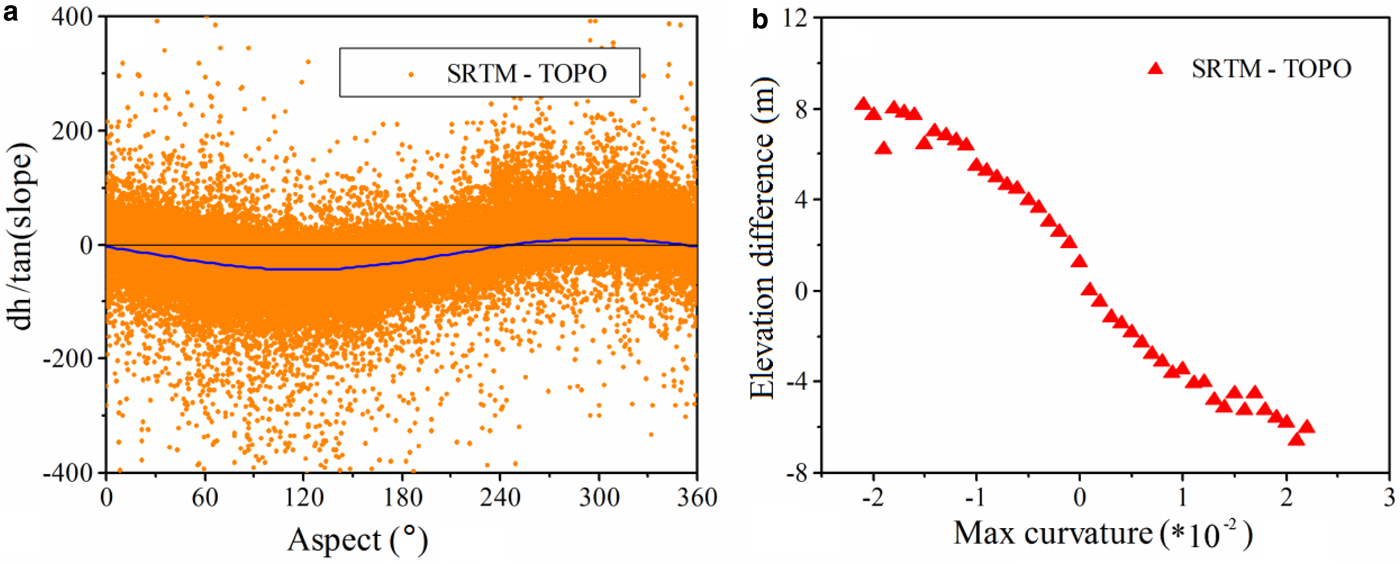
Fig. 2. Scatterplots of (a) aspect vs slope standardized elevation differences and (b) maximum curvature vs elevation difference in the CNR.
A difference map between SRTM and TerraSAR-X/TanDEM-X DEM was constructed by common DEM differencing. Based on the cosinusoidal relationship between elevation difference, slope and aspect, the vertical biases and horizontal displacements were rectified. Because TerraSAR-X/TanDEM-X DEM was created by the DInSAR method to optimize SRTM, both DEMs feature the same grid posting and are horizontally aligned. After these adjustments, the mean elevation difference in off-glacier regions was 0.80 m, which is slightly larger than 0.79 m that estimated by the DInSAR method.
3.4. Penetration depth
When the SRTM DEM is used for geodetic mass-balance calculations, the penetration depth of the radar signal into snow and ice has to be considered (Rignot and others, Reference Rignot, Echelmeyer and Krabill2001; Berthier and others, Reference Berthier, Arnaud, Vincent and Rémy2006; Gardelle and others, Reference Gardelle, Berthier and Arnaud2012a; Vijay and others, Reference Vijay and Braun2016; Neelmeijer and others, Reference Neelmeijer, Motagh and Bookhagen2017). Previous studies have indicated that the penetration depth is affected by the carrier frequency, the density of snow and ice and its water content (Berthier and others, Reference Berthier, Arnaud, Vincent and Rémy2006; Kääb and others, Reference Kääb, Treichler, Nuth and Berthier2015). Given that the TerraSAR-X/TanDEM-X were observed mostly in February, when the SRTM was performed, and the carrier frequencies of the TerraSAR-X/TanDEM-X and the SRTM X-band satellites are almost the same, it is assumed that penetration depths will be similar between these two datasets and can be neglected (Li and Lin, Reference Li and Lin2017). As a first approximation, because the penetration depth of the SRTM X-band radar beam is much smaller than the C-band, the elevation difference between SRTM C-band and X-band DEMs on glacier can be considered to be the SRTM C-band radar beam penetration into snow and ice (Gardelle and others, Reference Gardelle, Berthier and Arnaud2012a). As the acquisition date of SRTM avoided the main rainy season (Yang and others, Reference Yang2013), the penetration of radar signal would not occur in off-glacier regions, so elevation differences between SRTM C-band and X-band DEMs could be evaluated with common DEM differencing. At first, a difference map was constructed with SRTM C-band and X-band DEMs. Before adjustments, outliers are excluded using 5 and 95% quantile thresholds based on statistical analysis. Then, based on the substantial cosinusoidal relationship between standardized vertical bias and topographical parameters (slope and aspect), the vertical biases and horizontal displacements were rectified. After these adjustments, elevation differences between SRTM C-band and X-band DEMs on glacier can be considered to be the SRTM C-band radar beam penetration depth.
The penetration depth differences were analyzed and corrected in each 100 m elevation bin on glacier. Because the penetration difference should not exceed 10 m (Gardelle and others, Reference Gardelle, Berthier and Arnaud2012a), all of the difference values >±10 m were defined as outliers and were not considered for the penetration estimation. The median values of each elevation bin were used to correct the SRTM C-band DEM but only for areas with elevations below 6200 m a.s.l. In the CNR, the penetration depth difference for clean ice/firn/snow was ~0.88 m below 5200 m, and 1.28 m between 5200 and 6200 m. SRTM X-band DEM does not cover higher elevation region and penetration depth difference cannot be determined for regions above 6200 m. According to the linear trend calculated for the several highest bins in Figure 3, a value of 2.26 m was assumed for the area above 6200 m. For the debris-covered region, we did not apply any penetration corrections. In total, the average penetration depth of the SRTM C-band radar is 1.16 m for clean ice/firn/snow in the CNR. This value is consistent with previous studies finding an average penetration depth of 1.1 m in Yigong Tsangpo (Zhou and others, Reference Zhou, Li, Li, Zhao and Ding2018).
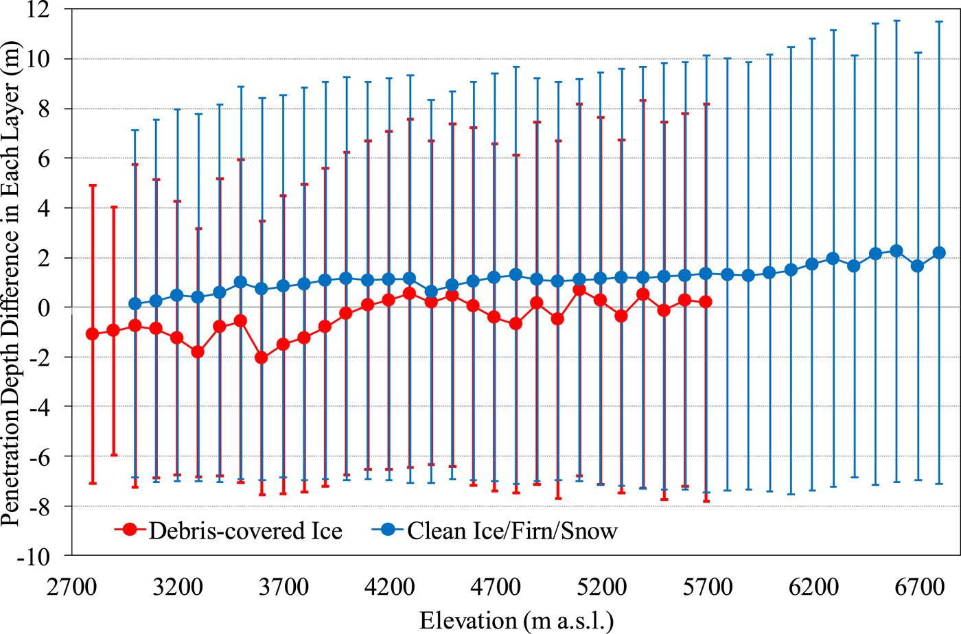
Fig. 3. Penetration depth differences between SRTM C-band and X-band DEMs at each elevation bin, red indicates debris-covered ice, while blue indicates clean ice/firn/snow.
3.5. Mass balance and accuracy estimation
In order to convert glacier-elevation changes to a geodetic mass balance, the glacier area and ice/firn/snow density must be considered. The geometric union of the 1968 and 2013 glacier masks was employed to respect maximum glacier extent between the dates of data acquisition (Li and others, Reference Li, Xing, Liu, Zhou and Huang2012; Neckel and others, Reference Neckel, Braun, Kropáček and Hochschild2013). An ice/firn/snow density of 850 kg m−3, with an uncertainty of 60 kg m−3, was applied to assess the w.e. of mass changes from elevation differences (Huss, Reference Huss2013; Wei and others, Reference Wei2015; Li and others, Reference Li, Lin and Ye2018).
Elevations from the ICESat Geoscience Laser Altimeter System (GLAS) were employed for a first accuracy assessment. These data are freely available from the National Snow and Ice Data Center (NSIDC) (release 634; product GLA14). Surface elevations of the DEMs were extracted at each ICESat footprint location. To ensure the accuracy of comparison, ICESat points were removed from the analysis if the elevation difference between GLA14 and multi-source DEMs exceeded 100 m in off-glacier region. A mean and SD of 2.14 ± 1.46 m and 1.95 ± 1.76 m in off-glacier regions were found for the TOPO and SRTM C-band DEMs, respectively. The GCPs used to convert the unwrapped TerraSAR-X/TanDEM-X interferogram into absolute heights from off-glacier pixel locations revealed that the vertical biases of the TerraSARX/TanDEM-X DEM and GLA 14 were similar to those of the SRTM C-band DEM and GLA 14.
To estimate the error in derived surface elevation changes, the residual elevation differences in off-glacier regions was calculated. The average elevation differences (AED) between the final difference maps in off-glacier regions ranged from −1.23 to 1.12 m (Table 3, Supplementary Fig. S1). The SD in off-glacier regions will probably overestimate the uncertainty of the larger sample because averaging in larger regions reduces the error. The uncertainty can be estimated by the standard error of the mean (SE) (Berthier and others, Reference Berthier, Schiefer, Clarke, Menounos and Rémy2010):
 $${\rm SE} = {\rm SD}/\sqrt N $$
where N is the number of the included pixels. To minimize the effect of autocorrelation, a decorrelation length based on the spatial resolution is recommended. For DEMs with a spatial resolution of 5 m, a decorrelation length of 100 m is suitable (Koblet and others, Reference Koblet2010). Bolch and others (Reference Bolch, Pieczonka and Benn2011) used values of 600 m for the spatial resolution of 30 and 400 m for 10–20 m. In this study, decorrelations of 600 and 200 m were employed for different DEMs with the spatial resolution of 30 and 10 m. The extent of study area was divided into several pixels according to the decorrelation length, N in Eqn (2) is the number of the included pixels in off-glacier area. In order to calculate the SE for a reasonable number of gridcells close to the glacier, only gridcells that located in a 5 km buffer around the glaciers were employed. The overall errors of derived surface-elevation changes can then be estimated using SE and AED in off-glacier regions:
 $$\sigma = \sqrt {{\rm AE}{\rm D}^2 + {\rm S}{\rm E}^2} $$
Table 3. Statistics of vertical errors between the TOPO, SRTM and TSX/TDX
AED, average elevation difference; STDV, standard deviation; SE, standard error.
* N, the number of considered pixels.
† σ, the overall error of the derived surface elevation change.
Finally, the overall mass-balance errors were determined using the estimated errors of glacier area and surface elevation change, and the ice density uncertainty of 60 kg m−3:
 $$Err_{MB} = \; (\sigma A_{max} + \; (\Delta H + \; \sigma )\; Err_{area})\; \rho $$
where Err MB is the overall errors of mass balance, σ is the overall errors of glacier elevation changes, ΔH is the mean glacier elevation changes, A max is the maximum glacier extent between 1968 and 2013, Err area is the overall errors of glacier area and ρ is the ice density of 910 kg m−3.
4 RESULTS
4.1. Area change
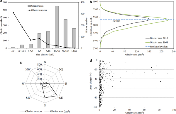
There were 715 glaciers with a total area of 1713.42 ± 51.82 km2 in 2016 in the CNR (Fig. 4). While large glaciers dominate the area (those >1 km2 occupy 93.5% of the total area) small glaciers dominate the number (those ≤0.5 km2 occupy 69.4% of the total number) (Fig. 4a). Approximately 82.2% of the total glacier area is found between 4500 and 5800 m of elevation, 4.9% is below 4200 m, and only 2.4% above 6200 m. The median elevation is ~5248 m (Fig. 4b). Kyagqen Glacier, the largest glacier (153.07 ± 0.43 km2) has the lowest tongue at 2882 m a.s.l. The mean glacier surface slope in the CNR is 22.8°, with most in the 12–32° range, accounting for 93.5% of total area. Glaciers having a SE, S or E aspect account for 85.5% of their area (Fig. 4c).
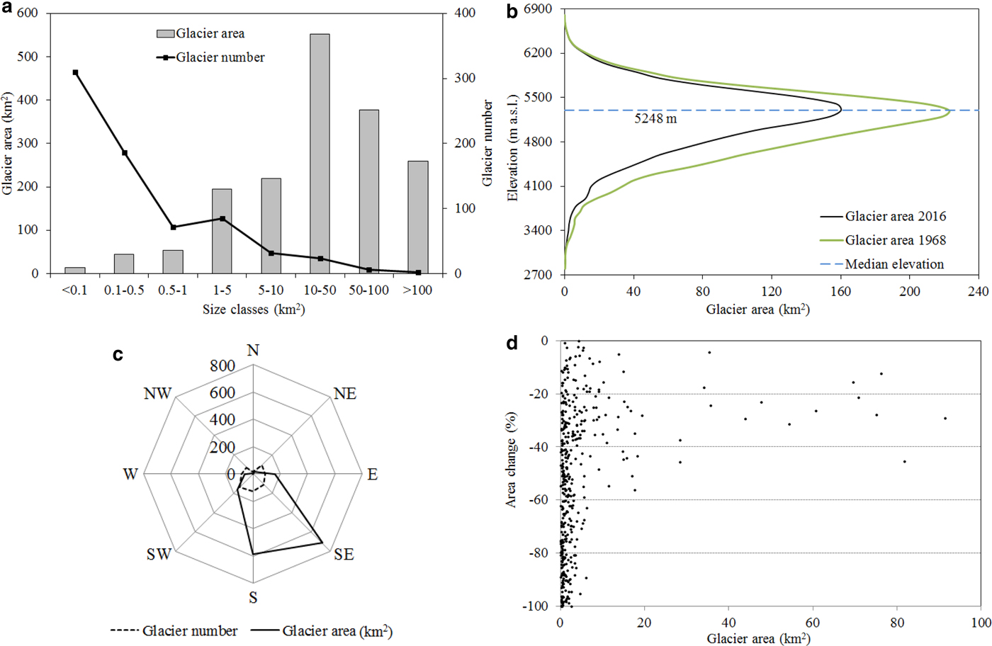
Fig. 4. Glacier distribution and change in the CNR. (a) Number and area of 2016 glaciers in different size categories. (b) Hypsography of glaciers in 1968 and 2016; the dashed line depicts the 2016 median elevation value. (c) Number and area of 2016 glaciers with different aspects. (d) Percentage change of glacier area from 1968 to 2016.
The CNR contains almost 100 glaciers with significant debris cover. The total debris-covered area of 203.23 km2 represents ~11.9% of the total glacierized area (Fig. 5). Among all the debris-covered glaciers, there were 12 glaciers with areas of debris cover that exceeded 5 km2. Nalong Glacier has the most in the CNR, 21.88 km2 or ~28.0% of its area. On Kyagqen Glacier, the debris cover only accounts for 3.2% of its area. Some 89.4% of the debris-covered area is in the 3700–5100 m elevation range, 7.4% is below 3700 m, and only 3.2% above 5100 m. The lowest elevation of debris cover (2882 m) coincides with the lowest limit of Kyagqen Glacier. The upper limit of debris cover (5754 m) is on Glacier 5N225E0033, on the north slope of the CNR.
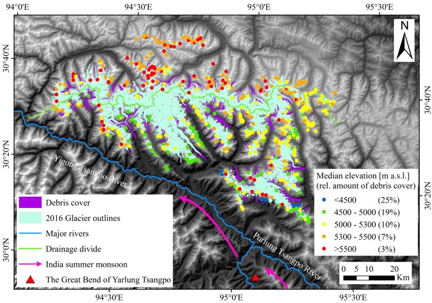
Fig. 5. Median glacier elevation and relative amount of debris cover is spatially correlated: median elevation is increasing from southeast to northwest, whereas the debris cover (indicated by the number in brackets in the legend) is decreasing along this gradient. The background map is SRTM DEM.
Comparing the total area of all glaciers in 1968 with that in 2016, ice cover in the CNR has diminished by 824.32 ± 55.65 km2 (32.5 ± 2.2%) or 0.68 ± 0.05% a−1 (Table 4). Small glaciers shrank the most, but large glaciers dominated the absolute area loss (Fig. 4d). Analysis of glacier hypsography showed that the ice cover below 2800 m, with an area of 0.32 km2, had disappeared completely, absolute area loss increased gradually with altitude through the 2800–5200 m a.s.l. range, then decreased gradually from 5200 to 6200 m a.s.l., remaining almost unchanged above 6200 m. Glaciers with lower elevation tended to lose relatively more area than higher elevation glaciers (Fig. 4b). The average minimum elevation of the glaciers increased by 258 m, while their median elevation rose ~97 m from 5151 to 5248 m. Disintegration of glaciers into smaller bodies of ice compensated for the disappearance of a few glaciers so the overall number of glaciers increased. Those that had disappeared were small and situated at relatively low altitudes.
Table 4. Glacier area changes in the CNR from 1968 to 2016
4.2. Mass balance
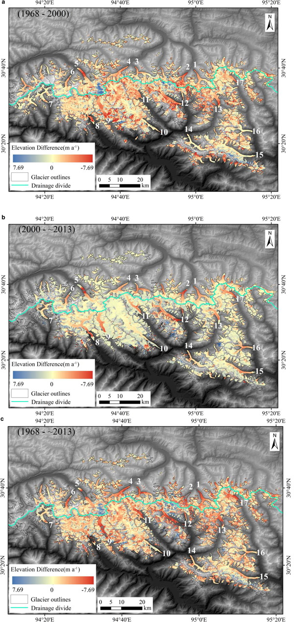
Significant glacier surface lowering has been observed in the CNR since 1968 with mass losses tending to increase during the most recent decade. Glaciers, with an area of 2624.30 km2 (the geometric union of the 1968 and 2016 glacier areas), experienced a mean thinning of 24.48 ± 0.70 m, or a mean mass loss of 0.46 ± 0.10 m w.e. a−1, equivalent to an overall mass loss of 64.21 ± 1.10 Gt from 1968 to 2013. The rate of thinning increased during the investigated periods. Glaciers thinned by 0.49 ± 0.22 m a−1, representing a mean mass loss of 0.42 ± 0.20 m w.e. a−1 from 1968 to 2000. Surface lowering was 0.71 ± 0.22 m a−1 with a mean mass loss of 0.60 ± 0.20 m w.e. a−1 from 2000 to 2013 (Fig. 6 and Supplementary Table S1). More details of elevation change are shown in Supplementary Figures S2–S5.
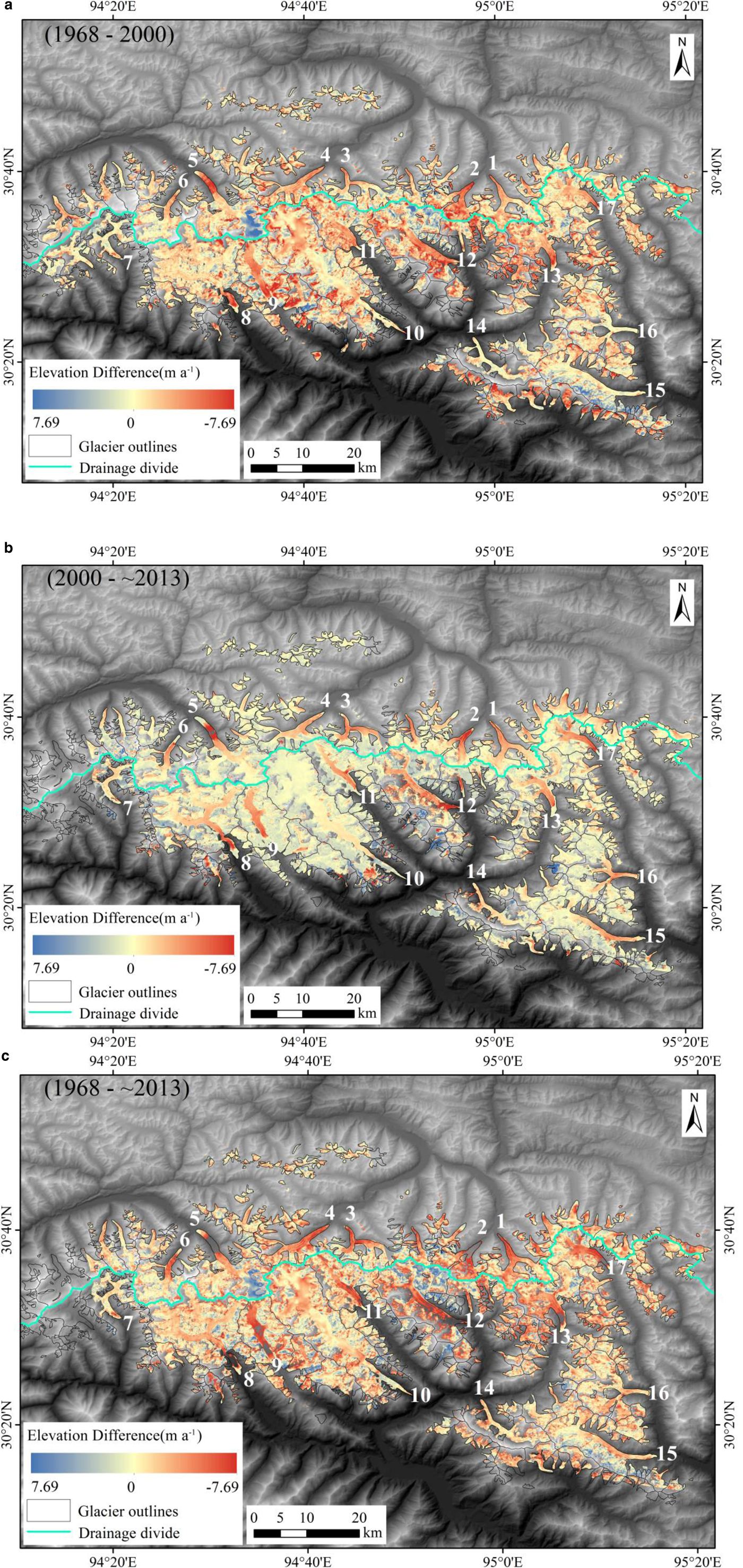
Fig. 6. Elevation changes in the CNR from 1968 to 2013. The glacier outlines are based on the geometric union of the 1968 and 2016 glacier extents. The background map is SRTM DEM. Numbers indicate specific sample glaciers chosen for analysis. (a) Elevation change from 1968 to 2000; (b) elevation change from 2000 to 2013 and (c) elevation change from 1968 to 2013.
Glaciers on the south slope, with an area of 1896.36 ± 20.39 km2, experienced a mean mass loss of 0.46 ± 0.09 m w.e. a−1 from 1968 to 2013, with means of 0.42 ± 0.19 m w.e. a−1 and 0.56 ± 0.17 m w.e. a−1 for 1968–2000 and 2000–2013, respectively. Losses of 0.48 ± 0.08 m w.e. a−1 on the north slope were close to those on the south slope from 1968 to 2013. Glaciers with an area of 727.94 ± 4.31 km2 in the former experienced a mean mass loss of 0.40 ± 0.20 m w.e. a−1 from 1968 to 2000, and then increased significantly to 0.72 ± 0.31 m w.e. a−1 from 2000 to 2013.
Changes varied significantly between the different time intervals and individual glaciers, even for those in the same basin with a similar climate. In 5O28 basin, Star Glacier (5O282A0103) experienced the largest mass loss from 1968 to 2013 (0.62 ± 0.11 m w.e. a−1) with losses much higher in the later period from 2000 to 2013 (1.09 ± 0.29 m w.e. a−1). Meanwhile Cape Glacier (5O282A0071), in the same drainage basin, experienced the smallest losses (0.24 ± 0.11 m w.e. a−1) from 1968 to 2013, with even less from 1968 to 2000 (0.07 ± 0.21 m w.e. a−1). Accelerating mass losses occurred on most sample glaciers, except for one glacier in the 5N225E basin and two in 5O281B, where the rate of mass loss decreased.
5 DISCUSSION
5.1. Uncertainty
The error in the derived glacier mass balance can result from both systematic and random components (Li and others, Reference Li, Lin and Ye2018). The latter comes from the precision of TerraSAR-X/TanDEM-X acquisitions, SRTM DEMs and TOPO DEMs, as well as the total glacier area measured. The systematic component includes errors in the seasonal effects and penetration depth.
Since geodetic measurements should determine mass balances ideally corresponding to an integer number of balance years, the seasonal variance of glacier mass balances needs to be considered (Gardelle and others, Reference Gardelle, Berthier and Arnaud2012b). In the CNR, maritime (temperate) glaciers develop and receive abundant summer monsoon precipitation. Most accumulation and melting occur simultaneously in the summer. TerraSAR-X/TanDEM-X and SRTM DEMs are acquired in February, and TOPO DEMs are acquired in April. To evaluate seasonal effects, glacier mass budgets determined from TOPO DEMs and TerraSAR-X/TanDEM-X or SRTM DEMs should be adjusted to the state of glaciers in February based on mass-balance variations. The annual distribution of mass balance is difficult to establish in the study area because field measurements are lacking. It has been assumed, conservatively, that precipitation is totally converted into mass accumulation. Based on the Dataset of Daily 0.5° × 0.5° Grid-based Precipitation in China (V2.0), the total precipitation in the study area from February to April in 1968 was 321 mm, which could create errors of up to ~0.01 m w.e. a−1 for the mass balances of 1968–2000 and 1968–2013. Compared with other factors in this study, any errors arising from the seasonal variance of mass balances can be considered negligible.
Another critical unknown is C-band radar penetration into snow and ice when SRTM C-band DEMs are used for geodetic mass-balance calculations. Penetration depths of 2.1–4.7 m at 10 GHz were measured in the Antarctic (Davis and Poznyak, Reference Davis and Poznyak1993), where the depth decreases as the temperature and water content of the surface snow increases (Surdyk, Reference Surdyk2002). Glaciers in the CNR are predominantly influenced by the monsoon and have higher snow moisture and temperatures than the Antarctic (Shi and Liu, Reference Shi and Liu2000). Hence, the assumption is that the penetration of the X-band radar is small, the difference between SRTM C- and X-band DEMs were used to estimate the absolute penetration of C-band. In total, the average penetration depth of the SRTM C-band radar is 1.16 m for clean ice/firn/snow in the CNR. This value is slightly smaller than that of Gardelle and others (Reference Gardelle, Berthier, Arnaud and Kääb2013), however, its possible penetration can be considered. The correction for C-band radar penetration led to average mass changes of +0.03 m w.e. a−1 for 1968–2000 and −0.08 m w.e. a−1 for 2000–2013.
5.2. Glacier inventory and changes of glacier area
The median elevation of a glacier is widely used to estimate the long-term equilibrium line altitude (Braithwaite and Raper, Reference Braithwaite and Raper2009), and is suitable for analyzing the governing climatic conditions (Ke and others, Reference Ke2016). Heterogeneous median elevations were detected in the CNR, and the spatial distribution of them reflects their climate dependence. This study area is located north of the Yarlung Tsangpo River where an important moisture transport path of the South Asian monsoon enters the plateau. From the Great Bend of the Yarlung Zangbo, the median elevation increases in SE–NW directions (Fig. 5). On the SE slope of the CNR, the South Asian monsoon brings abundant moisture, resulting in a relatively maritime climate and a lower median glacier elevation (below 5000 m). Because the high-mountain ranges block water vapor transport to the leeward side, a higher median glacier elevation (above 5300 m) is found on the NW slope. Conversely, if we classify the glaciers by median elevation first and then calculate the average debris cover for each class, it is found that the amount of debris cover for the median elevation classes decreases from 25.2% on the SE slope (median elevation <4500 m) to only 2.9% on the NW slope (median elevation >5500 m). The main reasons for this are probably an intensive debris supply from the steep rock walls facing south, the different geology of the SE and NW slopes, and autocorrelation effects between glaciers and the debris cover, i.e. the high amount of debris cover on low elevation glacier parts can be caused by the insulating effect of the debris itself (Kääb, Reference Kääb2005; Frey and others, Reference Frey, Paul and Strozzi2012; Ke and others, Reference Ke2016). Due to the insulating effect of the debris cover, the glacier terminus retreats more slowly. The amount of debris cover on the SE slope is larger than that on the NW slope, resulting in lower elevation glacier termini and a lower median glacier elevation on the SE slope than that on the NW slope.
Due to the influence of the South Asian monsoon, the CNR was almost permanently covered by snow and cloud, so the higher-quality optical-satellite images were rarely available from 2000 to 2010. Using 356 Landsat ETM+ scenes in 226 path-row sets from 1999 to 2003, Nuimura and others (Reference Nuimura2015) compiled the GAMDAM inventory (Glacier Area Mapping for Discharge from the Asian Mountains). There was a larger discrepancy between this and the 2000 CGI in the western Nyainqentanglha Range, probably because the GAMDAM inventory excluded thin ice on headwalls, the effects of shadow and seasonal snow cover, and tended to include smaller areas than those recommended by the GLIMS guidelines (Arendt and others, Reference Arendt2015; Wu and others, Reference Wu2016). An improved glacier inventory of the SE Tibetan Plateau (SETPGI) was compiled from Landsat images acquired from 2011 to 2013, coherence images from ALOS/PALSAR images and the SRTM DEM (Ke and others, Reference Ke2016). Comparing the SETPGI with our 2016 inventory, a slight discrepancy of glacier area (3.7%) was found which can be accounted for by a change in glacier area of −0.62% a−1 from 2010 to 2016. Meanwhile comparing the SETPGI with our 1968 inventory, ice cover in the CNR has diminished by −0.75% a−1 from 1968 to 2010. It was concluded that the glaciers in the study area have shrunk continuously since 1968 (−0.75% a−1 from 1968 to 2010 and 0.62% a−1 from 2010 to 2016), although the rate has eased during the most recent decade. The main reasons for this eased tendency are probably the effect of debris cover, which slowdown the retreat of glacier terminus.
5.3. Changes of glacier elevation and mass balance
Previous studies agreed that glaciers in the CNR were losing mass, though results differed from each other. Based on SRTM and SPOT5 DEMs (24 November 2011), a mean thinning of 0.39 ± 0.16 m a−1 was found between 2000 and 2011 by Gardelle and others (Reference Gardelle, Berthier, Arnaud and Kääb2013), whereas different rate of 1.34 ± 0.29 m a−1 from 2003 to 2008 was recorded over the CNR by Kääb and others (Reference Kääb, Treichler, Nuth and Berthier2015), using ICESat and SRTM. In this study, SRTM DEM and TerraSAR-X/TanDEM-X acquisitions yielded a mean thinning of 0.54 ± 0.05 m a−1 from 2000 to 2013. At a first glance, this result agrees with Gardelle and others (Reference Gardelle, Berthier, Arnaud and Kääb2013) but has significant difference from Kääb and others (Reference Kääb, Treichler, Nuth and Berthier2015). Different estimates of SRTM C-band penetration have resulted in thinnings at variance with those determined by Kääb and others (Reference Kääb, Treichler, Nuth and Berthier2015). An average SRTM C-band penetration of 8–10 m (7–9 m when based on winter trends assumed to reflect February conditions) was used for the eastern Nyainqentanglha Mountains in the Kääb and others (Reference Kääb, Treichler, Nuth and Berthier2015) study, much greater than the 1.7 m assumed in the study of Gardelle and others (Reference Gardelle, Berthier, Arnaud and Kääb2013) and 1.16 m assumed in this study. Previous studies suggested an average penetration of 2.4 m in Bhutan and 1.4 m around the Everest (Gardelle and others, Reference Gardelle, Berthier, Arnaud and Kääb2013), 2.26 m for clean ice below 6000 m in the Mount Everest region (Li and others, Reference Li, Lin and Ye2018), 2.5 ± 0.5 m for a wider area including east Nepal and Bhutan (Kääb and others, Reference Kääb, Berthier, Nuth, Gardelle and Arnaud2012), 1.67 ± 0.53 m in the western Nyainqentanglha Mountains (Li and Lin, Reference Li and Lin2017) and 1.24 m in the Kangri Karpo Mountains (Wu and others, Reference Wu2018). Because the CNR lies in the center of the eastern Himalaya, western Nyainqentanglha Mountains and Kangri Karpo Mountains, the characteristics of glacier in the CNR are similar to the surrounding regions (Shi and Liu, Reference Shi and Liu2000). Since penetration depth varies with temperature and water content (Surdyk, Reference Surdyk2002), an average penetration of 1.16 m, in agreement with previous studies, was deemed acceptable and suitable for estimating glacier elevation changes in the CNR.
Brun and others (Reference Brun, Berthier, Wagnon, Kääb and Treichler2017) recorded a mean mass loss of 0.62 ± 0.23 m w.e. a−1 between 2000 and 2016 in the Nyainqentanglha Range, based on ASTER optical satellite stereo pairs. Because this result relies exclusively on satellite optical data, it is not affected by signal penetration. Our determination of a mean mass loss of 0.60 ± 0.20 m w.e. a−1 from 2000 to 2013 in the CNR agrees with that Brun and others (Reference Brun, Berthier, Wagnon, Kääb and Treichler2017) and suggests our results are reliable. A larger discrepancy is noted with the Zhou and others (Reference Zhou, Li, Li, Zhao and Ding2018) results in Yigong Tsangpo from declassified KH-9 images (21 December 1975) and SRTM DEMs; 0.11 ± 0.14 m w.e. a−1 vs our result of 0.42 ± 0.20 m w.e. a−1 from 1968 to 2000. There are likely three reasons for this discrepancy: first, a difference in dates of the declassified KH-9 images and topographic maps; second, a difference in the glacier area measured. The Yigong Tsangpo study measured a glacier area of 1055 km2 while ours was 2622.95 km2. Third, there are differences in how data voids in the accumulation area are filled.
Ice in the comparatively flat lower parts of the larger valley glaciers is much thicker than that in the steep higher glacier reaches, due to the generalized flow law of ice (assumption of perfect plasticity) (Cuffey and Paterson, Reference Cuffey and Paterson2010). In other words, a large amount of the glacier volume is stored in the low-lying ablation regions, as median elevation separates glaciers in two halves of equal size. This suggests that large amounts of ice can become subject to melt in the event of climate warming. Whereas the mass-loss patterns on a debris-covered tongue are complicated, with supraglacial lakes, ice cliffs and heterogeneous debris cover (Pellicciotti and others, Reference Pellicciotti2015). Although it is generally believed that ablation rates are retarded with a thick debris cover due to its insulating effect (Benn and Lehmkuhl, Reference Benn and Lehmkuhl2000), some previous studies have found that ablation is greater when the debris is less than a critical thickness (Zhang and others, Reference Zhang, Fujita, Liu, Liu and Nuimura2011, Reference Zhang2016; Ye and others, Reference Ye2015). In this study, the surface properties have a positive influence on the melt: thinning was noticeably greater on the debris-covered ice than the clean ice in the 2800–5700 m a.s.l. range from 1968 to 2013 in the CNR (0.92 ± 0.10 vs 0.51 ± 0.10 m a−1) (Fig. 7). Similar results have been found in the eastern Pamir (Zhang and others, Reference Zhang2016), the Karakoram (Gardelle and others, Reference Gardelle, Berthier and Arnaud2012b), the western Himalaya (Berthier and others, Reference Berthier2007; Frey and others, Reference Frey, Paul and Strozzi2012) and the Mount Everest region (Bolch and others, Reference Bolch, Buchroithner, Pieczonka and Kunert2008).
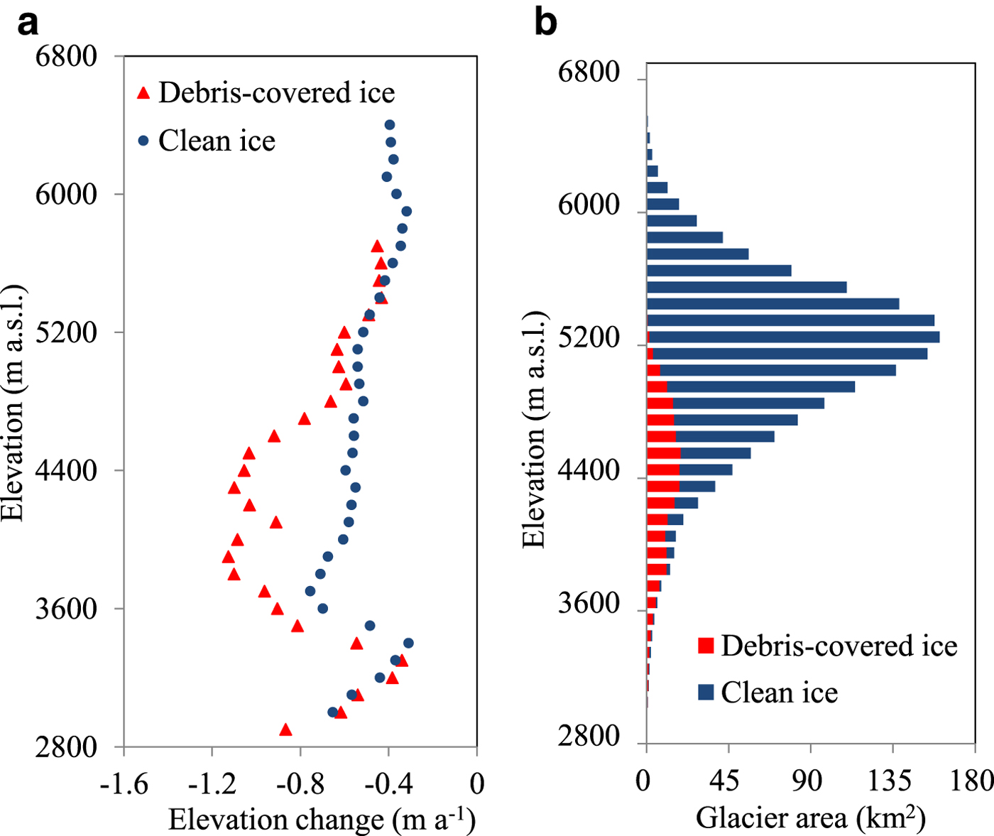
Fig. 7. Glacier elevation changes and distribution of 2016 glacier area at each 100 m interval by altitude in the CNR for clean ice and debris-covered ice from 1968 to 2013.
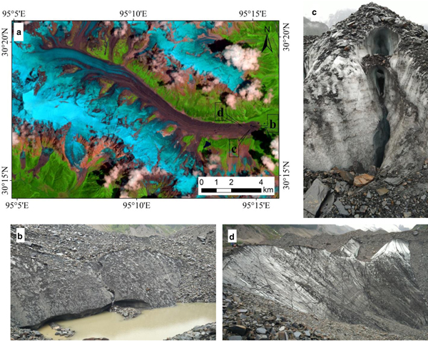
Apart from debris cover, there are other features that may affect surface elevation changes, such as supraglacial/proglacial lakes, and ice cliffs. Although ice cliffs account for a small proportion of the total debris-covered area, they can make a disproportionate contribution to total ablation (Sakai and others, Reference Sakai, Nakawo and Fujita2002; Han and others, Reference Han, Wang, Wei and Liu2010; Benn and others, Reference Benn2012). On steep slopes, heavy debris slides off leaving very fine debris on the ice cliffs. This reduces the ice albedo so the cliffs absorb more shortwave radiation, which is augmented by longwave radiation from the adjacent warm debris layers (Reid and Brock, Reference Reid and Brock2014). Figure 8 shows the debris cover on Cape Glacier, its ice cliffs, and supraglacial lake. Compared with the clean ice in the 2800–5700 m a.s.l. range in the CNR, the thin debris cover, exposed ice cliffs and supraglacial/proglacial lakes would contribute to the greater thinning rate observed on debris-covered glaciers in the CNR.

Fig. 8. The debris-covered tongue of Cape Glacier with supraglacial lakes and ice cliffs: (a) the background image is a Landsat OLI image (4 Aug 2013, RGB:743. The letters on the tongue of Cape Glacier correspond to photo panels in this figure); (b) supraglacial lake; (c) and (d) ice cliffs (photos taken by K. P. Wu, 12 June 2015).
Different thinning rates were detected for land-terminating glaciers and lake-terminating glaciers in the CNR. Land-terminating glaciers with heavy debris-covers (5N225E0005, 5N225E0031, Yenong, Xiaqu, Kyagqen, Nalong, Maguolong, Yangbiegong, Cape and North Cape) experienced a mean thinning of 0.53 ± 0.10 m a−1 from 1968 to 2013, which was smaller slightly than the regional average (0.54 ± 0.10 m a−1). Surface lowering of all lake-terminating glaciers (5N225E0010, 5N225E0033, Jiongla, Lepu, Daoge, Ruoguo and Star) was 0.62 ± 0.10 m a−1, or higher than the regional average. These results are in agreement with previous studies of surface thinning on land and lake-terminating glaciers (Neckel and others, Reference Neckel, Loibl and Rankl2017; Li and others, Reference Li, Lin and Ye2018).
5.4. Climate change
Based on temperature data from 79 meteorological stations on the TP, the SE TP was the area with the least warming, compared with the rest of the TP (Duan and others, Reference Duan, Li and Fang2015). Conversely, the MODIS land surface temperature (MODIS LST) showed that the SE TP experienced the most warming (Yang and others, Reference Yang2014). The National Centers for Environmental Prediction/National Center for Atmospheric Research (NCEP/NCAR) reanalysis data results indicated a decreasing trend of average annual temperature during 1961–2004 (You and others, Reference You2010). Similarly with precipitation, a negative trend in the SE TP was shown by Global Precipitation Climatology Project (GPCP) data (Yao and others, Reference Yao2012), while a positive trend came from Chinese meteorological station annual precipitation data (Li and others, Reference Li, Yang, Wang, Zhu and Tang2010). Thus, glacier changes in the CNR cannot be related directly to these contrasting summaries of climate information.
To analyze the response of glaciers in the CNR to climate change, relevant air temperature and precipitation datasets were taken from the Dataset of Daily 0.5° × 0.5° Grid-based Temperature/Precipitation in China (V2.0) (Dataset2.0). Using the thin plate smooth spline method, and a 50 year (1961–2010) quality controlled observational daily temperature and precipitation data series based on 2472 gages (http://data.cma.cn/data/cdcindex/cid/00f8a0e6c590ac15.html), Dateset2.0 was produced by the Climate Data Center, National Meteorological Information Center, China meteorological Administration for Mainland China. A previous study showed that the mean bias error of precipitation in most gages is between −1 and 1 mm d−1 (Zhao and Zhu, Reference Zhao and Zhu2015). Dataset2.0 underestimates the rain intensity during heavy or moderate rainfall events. Over the light rain, it has more veracity. Dataset2.0 describes the climate characteristic of the TP, the Tienshan Mountains and Tarim Basin (Zhao and Zhu, Reference Zhao and Zhu2015).
To calculate temperature and precipitation trends between 1961 and 2010, linear regression analysis was performed for each gridcell. Figure 9 shows the horizontal distribution of surface temperature and precipitation changes from May to September since 1961, with a confidence level <0.1. It is clear that increasing surface temperatures and decreasing precipitation have been dominant in the CNR in recent decades. The changes in surface temperature and precipitation were confirmed with data from the three nearest meteorological stations, Jiali (30°40′ N, 93°17′ E, 4488 m a.s.l.), Bomi (29°52′ N, 95°46′ E, 2736 m a.s.l.) and Linzhi (29°40′ N, 94°20′ E, 2992 m a.s.l.). Surface temperature at these stations increased slightly from 1961 to 2000 and then significantly after 2000. Average temperatures at Jiali, Bomi and Linzhi station after 2000 increased 0.45, 0.67 and 0.86 °C than those before 2000, respectively. Trends in precipitation are not evident at the three stations, which present large interannual precipitation fluctuations (Fig. 10).
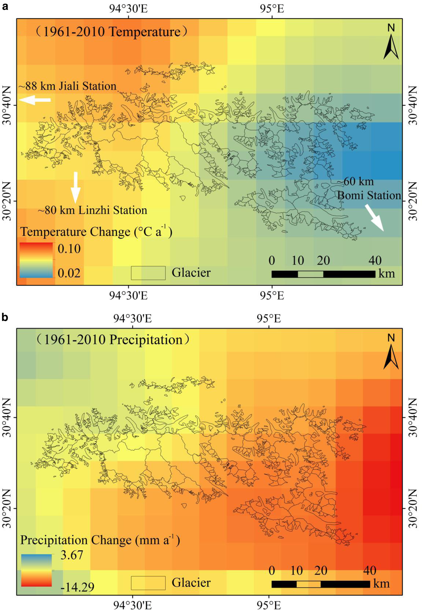
Fig. 9. The changes of temperature and precipitation (from May to September) in the CNR from Dataset2.0 during 1961–2010: (a) temperature and (b) precipitation.
Fig. 10. Annual variations of average temperature and precipitation (from May to September) around the CNR: (a) Jiali, (b) Bomi and (c) Linzhi, and linear trends are shown as black solid lines.
Dataset2.0 shows average precipitation decreasing by more than 4 mm a−1 since 1961, resulting in less glacier accumulation. The average surface temperature increased by more than 0.2 °C per decade in the CNR (with a confidence level <0.05), higher than the rate of global warming (0.12 °C per decade, 1951–2012) (IPCC, 2013). The reduced precipitation on the north slope is smaller than on the south slope, while the warming rate on the north slope is larger than that on the south slope. Therefore, the observed mass loss in the CNR is consistent with observed increases in temperature and decreases in precipitation. Analysis of drivers of sub-period glacier mass changes requires additional information and modeling. The mean mass loss before 2000 was smaller than that after 2000 in the CNR, glacier changes were consistent with climate warming. And the mass loss in the 5N22 drainage basin (on the north slope) was larger than that in the 5O28 drainage basin (on the south slope) during 2000–2013, resulting from the difference of precipitation decreasing. It is concluded that glacier mass loss in the CNR can be attributed to climate warming and precipitation decreasing.
6. CONCLUSION
Based on Topographical Maps, Landsat TM/ETM+/OLI images, SRTM and TerraSAR-X/TanDEM-X acquisitions, the changes of glacier area, surface elevation and mass balance in the CNR during recent decades have been estimated.
Results show that the CNR contained 715 glaciers, with a total area of 1713.42 ± 51.82 km2 in 2016. Ice cover has diminished by 0.68 ± 0.05% a−1 since 1968, but the rate of glacier shrinkage has lessened during the most recent decade. Compared with the recession of mountain glaciers in western China, those in the CNR have experienced extremely strong retreat. Overall, the area covered by debris accounts for 11.9% of the whole ice cover, with the coverage decreasing in SE–NW directions.
Significant surface lowering of glaciers has been observed since 1968, and mass losses have increased in recent decades. Thinning was noticeably greater on the debris-covered ice than the clean ice in the 2800–5700 m a.s.l. altitude range from 1968 to 2013. Aside from debris cover, other features increasing glacier surface melting include proglacial/supraglacial lakes, and ice cliffs. Observed glacier mass changes in the CNR region are consistent with increased temperatures and decreased precipitation observed from gridded meteorological observations.
SUPPLEMENTARY MATERIAL
The supplementary material for this article can be found at https://doi.org/10.1017/jog.2019.20
ACKNOWLEDGEMENTS
This work was supported by the fundamental program of the National Natural Science Foundation of China (grant no. 41801031), the Ministry of Science and Technology of China (MOST) (grant no. 2013FY111400), the project of State Key Laboratory of Cryospheric Science (grant no. SKLCS-OP-2019-07), the National Natural Science Foundation of China (grant nos. 41190084, 41671057, 41671075 and 41701087), the International Partnership Programme of the Chinese Academy of Sciences (grant no. 131C11KYSB20160061) and the grant for talent introduction of Yunnan University. Landsat images are from the US Geological Survey and NASA. The TerraSAR-X/TanDEM-X images are from the DLR. The GAMDAM glacier inventory was provided by A. Sakai. The first and second glacier inventories were provided by a recent MOST project (2006FY110200). The Dataset of Daily 0.5° × 0.5° Grid-based Temperature/Precipitation in China (V2.0) is from the China Meteorological Data Service Center (CMDC) in Beijing. All SAR processing was performed with GAMMA SAR and interferometric processing software. We thank DLR for free access to SRTM X-band data and USGS for free access to SRTM C-band and Landsat data.


 Open access