


Introduction
It is possible that in the near future the electrical properties of snow and ice may find various applications to glaciological problems in the field. Using established geophysical prospecting techniques, direct-current electrical resistivity measurements have already been used on polar and temperate glaciers to obtain some information about the depth of snow, and underlying rock type. This paper is concerned with alternating-current and radio-frequency properties of ice and snow. The information available in the literature has been collected with the intention of finding the gaps in present knowledge, and new experimental work directed to filling the gaps which appear to be of interest will appear in a later paper. Applications of the electrical properties to the measurement of ice thickness, temperature, mechanical stress, and crystal orientation, are indicated in this paper and it is hoped that further ideas will be stimulated. A complete annotated bibliography of published measurements is given in chronological order in Appendix A. In the text, references to other authorities have been kept to a minimum.
The Relaxation Spectrum
1.1. Pure ice
Many workers have investigated the large dielectric dispersion which occurs in ice at audio- and low radio-frequencies and it is therefore not our intention to treat this range or its relation to the molecular structure of ice in detail.
In general, measurements of various authors are in good agreement with one another and with the Debye equation for dielectrics consisting of polar molecules having a single relaxation time. This is a common type of spectrum and some of the important properties are given in Appendix B; the unusual features of ice are its extremely high static permittivity (of the order of 100) and its long relaxation time (of the order of 10−4 sec.). In comparing the various measurements there are a number of variables to be considered. Temperature is important because the relaxation time of all materials is increased as the temperature is reduced, the possible effect of impurities must be considered, and it is believed that mechanical stress may have an influence. If the medium considered is snow, then density is important because it is a mixture of two dielectrics, ice and air, and this introduces at least one further variable which characterizes the shape and orientation of the particles comprising the mixture.
Restricting ourselves to pure ice, free from cracks, bubbles, impurities, and stress, a representative Cole–Cole diagram at −11°C. is shown by curve (a) in Figure 1. The relaxation time, τ, can be related to absolute temperature, T, by the Boltzmann condition which gives
and Reference Auty and ColeAuty and Cole (1952) obtained values of τ 0 (the time constant) and E (the energy) for dipole orientation. When their values are substituted in (1) we obtain
and this relation has been used to plot the solid line in Figure 2 assuming the values of τ 0 and E to be substantially independent of temperature.

Fig. 1. Relative permittivity (abscissae) and loss factor (ordinates) of ice samples at − 10.8°C. (after Reference Auty and ColeAuty and Cole, 1952). Frequencies in kilocycles per second are marked against measured points (a) pure ice, free from cracks, bubbles, impurities, or stress; (b) with a crack perpendicular to the electric field reducing ϵs (c) with impurities, increasing the d.c. conductivity and increasing ϵs

Fig. 2. Frequency, for which the loss factor, ϵ″ is a maximum (abscissae) plotted logarithmically versus temperature (ordinates). The measurements of Reference Auty and ColeAuty and Cole (1952) are marked an the solid line which is computed from equation (2).▲ Laboratory measurements on pure ice by Reference LambLamb (1946); ■ Field measurements on Athabaska Glacier by Reference Watt and MaxwellWatt and Maxwell (1960); ● Natural snow samples from Sapporo City measured in the laboratory by Reference KuroiwaKuroiwa [1956]. The density in g./cm.3 is given alongside each point
The limiting value of permittivity at high frequency is found to be independent of temperature and equal to 3.15±0.05 but there is an increase in the low frequency or static value, from 92 to 103, in polycrystalline ice as the temperature is reduced from 0°C. to −45°C. and a steeper rise thereafter. Reference PowlesPowles (1952) has derived theoretical values for the static permittivity by considering a finite number of oxygen atoms in specific tetrahedral structures. He is able to include up to 24 atoms in an aggregate and to calculate the electric effect, and hence the contribution to the total polarization, of a single atom near the centre. Beyond 24 atoms the calculations become too long and the effect on the result small. The average dipole moment is then used in Fröhlich’s formula for the permittivity of a solid. Two results of Powles, on the assumption that all configurations of the aggregate are equally probable, and the alternative assumption that the probability is related to the electrostatic energy of the system, are shown in Figure 3 together with some experimental values. Careful measurements on individual crystals show that there is appreciable anisotropy. This was ignored, for simplicity, in Powles’ model but it may provide a means of examining the degree of crystal orientation by measuring the static permittivity in naturally occurring ice masses.

Fig. 3. Permittivity of ice at low frequencies (ordinates) against temperature in degrees centigrade (abscissae). ▲ Polycrystalline sample (Reference Auty and ColeAuty and Cole, 1952); ● Single crystal, electric field parallel to c-axis; ■ Single crystal, electric field perpendicular to c-axis; no pure real value at −5°C. (Reference HumbelHumbel and others, 1953). I and II: limiting cases from Reference PowlesPowles (1952) calculation
1.2. Snow
The behaviour of a mixture of dielectrics has been discussed by a number of authors who generally consider a sparse distribution of separate particles, of idealized mathematical shape, within a second dielectric medium (Reference WagnerWagner, 1913; Reference SillarsSillars, 1937; Reference Vieweg and GastVieweg and Gast, 1943). However Reference WeinerWeiner (1910) showed empirically that even in a dense distribution a single parameter, which he called the Formzahl, is often sufficient to describe how one medium is dispersed within the other. Basically this amounts to assuming that the geometry of the electric field is not a function of the relative proportion of the two media and this cannot be strictly true. It is easy to see that if the particles of the high-permittivity medium are elongated in the direction. of the electric field, the combined permittivity will be higher than if they lie across the field and the mixture may be anisotropie, requiring different Formzahl in different directions. A mixture of long thin particles, randomly orientated, will be isotropic in the mass but have a higher permittivity than a suspension of spherical particles having the same volume ratio. Some illustrative examples are given in Figure 4, and in Figure 1 curve (b) shows the effect of an air crack perpendicular to the electric field direction in an otherwise solid block of ice.
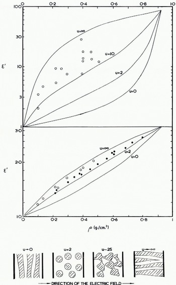
Fig. 4. Relative permittivity of snow (ordinates) versus density (abscissae). The upper turves are computed as explained in section 1.2 for snow particles having the characteristic Formzahl values u = 0, 2, 10, and ∞ in Weiner’s formula and taking the relative permittivity of solid ice to be 90 at low frequencies. The lower curves are for the limiting value of the permittivity at high, frequencies, taken to be 3.2 for solid ice. Measured values: O due to Reference KuroiwaKuroiwa [1956] at frequencies less than 1 kc. f sec. and at 3 Mc. sec., ● due to Reference CummingCumming (1952) at 9,375 Mc./set. The sketches beneath the graphs. show how snow structure is related to the Formzahl
Weiner found that if ϵ m , ϵ 1 and ϵ 2 are the relative permittivities of the mixture and the two separate media respectively then

where p is the proportion of the total volume occupied by medium 1 and u is the Formzahl. The formula includes the effect of losses if complex values are substituted for ϵ 1 and ϵ 2 but if the losses are such that tan2 δ ≪ 1 then only the real parts need to be substituted in equation (3) to find the real part of ϵ m , and in this section we restrict the application of the formula to the limiting values of permittivity at low and high frequencies, ϵ s and ϵ ∞ respectively. Furthermore, in the case of snow, medium 2 is air, ϵ 2 = 1+j0, and the second term on the right hand side of equation (3) is zero. Medium 1 is ice and thus p = ρ/0.92 where ρ is the specific gravity of the snow.
In Figure 4 independent measurements are compared with relationships computed from Weiner’s formula. Cumming’s results correspond to a Formzahl value between 2 and 4 whilst for Kuroiwa’s results a value greater than 10 is required. Cumming’s snow samples came from Ottawa, Canada, and Kuroiwa’s from Sapporo city, Japan, so that it would not be surprising if there had been more opportunity for bonds to form between the ice crystals by partial thawing and refreezing in Kuroiwa’s samples. They included new snow, compact snow, and granulated snow and he found in a separate investigation that the Formzahl value, u, increased with time. It is suggested that any values of u between 2 and infinity must be expected in practice according to the structure of the snow; the curves for these two values set some limit to the permittivity of snow of known specific gravity.
There is no obvious way in which the relaxation time should be related to snow density but the available measurements on snow of known specific gravity (due to Kuroiwa) all have shorter relaxation times than pure ice. In Figure 2 the experimental results are compared with a curve derived from the relaxation time of pure ice given by equation (2). G. de Q. Robin has suggested (private communication) that this relationship might be a basis for the measurement of temperature within large bodies of snow, and the method looks promising because the variation of frequency is so large. It will be necessary to establish that there are no important variables other than the temperature; Reference GränicherGränicher and others (1957) and Reference BrillBrill (1957) find that impurities in solid solution shorten the relaxation time and Westphal (private communication) finds that mechanical stress shortens the relaxation time. It would clearly be worth while to obtain measurements at lower temperatures on naturally occurring snow of known density and conductivity, and if possible, where some estimate of the stress can be made.
1.3. Effect of impurities and liquid water
The presence of impurities in small quantities, or of water when the temperature is near freezing point, may have two effects. First there is the effect on the permittivity due to the mixture of dielectric media as discussed above, and this is especially important if liquid water is present because the relative permittivity of water remains very high up to frequencies in the centimetre wavelength band. Values of permittivity at high frequency for a mixture of snow of specific gravity 0.5 (for which we take the real part of the permittivity at high frequency (ϵ′ = 2) and liquid water (ϵ′ = 80) have been calculated for various values of the Formzahl and the results are compared in Figure 5 with some measurements on wet snow of the same density. The results were published as deviations from the permittivity of dry snow, and there is clearly a systematic error in the measurement of free water content since there is a finite deviation when no measureable quantity of water is present; this is attributed to the inefficiency of the centrifugal separator used to extract the water. Reference AmbachAmbach (1963, p. 174–77) has proposed that measurement of the dielectric constant could be used to estimate the free water content of snow. However, the magnitude of the effect depends greatly on the specific gravity of the dry snow (which will not usually be known) and on the effective value of the Formzahl.

Fig. 5. Permittivity of wet snow at high frequencies (ordinates) versus volume percentage of liquid water (abscissae). The permittivity of the dry snow is assumed to be 2.0, corresponding to a specific gravity of approximately 0.5. The continuous lines are calculated from Weiner’s mixing formula and the measured values are due to Reference KuroiwaKuroiwa [1956]. There is a systematic error in his measurement of the free water content. Reference AmbachAmbach (1963, p. 174–77) has given results for snow of much lower density
The second consideration when impurities are present is the increased value of the direct-current conductivity, σ If the conductivity is known, or can be measured, then the contribution to the loss factor, ϵ″, may he calculated from the relationship in Appendix C. Some figures are given for natural snow in Table I; Kopp lists the widest range of samples and temperatures but it is interesting to compare his figures with others derived by entirely independent means. Those for impure city snow have been estimated by the reverse process to that mentioned above—by taking the deviation of ϵ″ from the semicircular form in Cole–Cole diagrams published by Kuroiwa for snow samples containing up to 30 parts per million of chloride ions among other impurities. The conductivity is high as would be expected. The low conductivities obtained by Watt and Maxwell for wet snow are more surprising, but they are believed to be entirely reliable since they are derived from consistent Cole-Cole plots measured with ELTRAN electrode arrays on the undisturbed material in the field. H. Röthlisberger reports (private communication) that it is now established that fine-grained Arctic snow has a higher conductivity than wet avalanche snow in Europe, for which values very close to those of Watt and Maxwell have been found.
Table I Direct-Current Electrical Conductivities

In the absence of experimental values of the conductivity in the required circumstances the best that can be done is to set some limits to the effect. Thus the d.c. conductivities of various waters and other materials are also listed in Table I together with the approximate frequency below which the loss tangent is greater than unity, that is, where the effect of the d.c. conductivity cannot in any circumstances be ignored. The surprising result here is the high conductivity of frozen earth, however there is good agreement between entirely independent measurements.
In cold ice with carefully controlled amounts of impurity, Reference GränicherGränicher (1963) found that concentrations of the order of a hundred parts per million of suitable atoms can exist in solid solution before the crystal lattice is disarranged with separate crystals and bubbles appearing. At this point, the limit of miscibility, the conductivity can be increased to about 10−3 mho per metre. There are large changes in permittivity for much lower concentrations, when the conductivity is about 10−5 mho per metre and this shows in curve (c) in Figure 1. The conductivity and increased permittivity arise from lattice imperfections and the contribution of various types of imperfections have been discussed by Reference HastedHasted (1961).
Radio Frequencies
2.1. Permittivity: Ice
Between a frequency of 1 Mc./sec. and the far infra-red region there is no absorption band in the spectrum of ice. We shall give the evidence for this statement below, but once the fact is established there is no further interest to the chemist in investigating the spectrum in the intervening region from the point of view of elucidating the crystal or molecular structure. The only incentive to experimental work is likely to come from a practical requirement for knowledge of the properties of ice or snow as a radio-frequency material in a particular application. One may be interested in radio propagation over snow-covered ground, over ice-covered water, or the effects of icing on antenna and transmission-line parameters. Consequently the available measurements are not easily compared with one another since they relate to samples differing in temperature, density, composition, and mechanical stress, factors which are not always adequately specified.
Let us consider first the relative permittivity of pure solid ice as a function of frequency. Results are collected in Figure 6 where code letters identify the individual authorities, the temperature, and other remarks about the measurements. At frequencies of the order of 1 Mc./sec. we expect to observe the high frequency tail of the relaxation spectrum, and this will be sensitive to temperature, the coefficient decreasing to zero with increasing frequency. The measurements of Lamb and Auty and Cole seem to represent the most recent and careful laboratory work on pure ice free from residual stress. The highest frequency plotted by Auty and Cole is 50 kc./sec. and the curve in Figure 6 is extrapolated to their published value of high-frequency permittivity using the Debye formula. Lamb’s measurements refer to a slightly higher temperature but the real difference between the two lies in the limiting values of the permittivity at high frequency, ϵ ∞ = 3.10 and 3.17 respectively. Lamb found the same value, 3.17, at 10,000 Mc./sec. and 24,000 Mc./sec. with negligible temperature coefficient in the range 0° to −190° Cumming’s results, 3.15 at 9,375 Mc./sec., and Von Hippel’s results, 3.17 at 10,000 Mc./sec. and 3.20 at 3,000 Mc./sec., are all in good agreement.

Fig. 6. Relative permittivity of ice (ordinates) versus logarithm of radio frequency (abscissae)
L: Reference LambLamb (1946) and Lamb and Turney (1949) −5°C. at low frequencies, 0° to −190°C. at high frequencies: distilled water.
C: Reference CummingCumming (1952) −18°C. Distilled water and melted snow.
A: Reference Auty and ColeAuty and Cole (1952) − 10°C. Conductivity water: ice free from stress.
V: Reference Von HippelVon Hippel (1954) −12°C. Conductivity water: ice not annealed.
Y: Reference YoshinoYoshino (1961) −18° to −36°C. Antarctic ice, not annealed, density 0.91 g./cm.3
W: Westphal (private communication) −5° to −60°C., annealed Greenland ice, density. 0.90g./cm3
Uncertainty arises in the intermediate range, 1 to 1,000 Mc./sec., where the measurements of Von Hippel on pure ice made in the laboratory from conductivity water, and recent measurements of Yoshino made in the Antarctic, lie much higher than would be expected from the results on either side. Westphal (private communication) states that Von Hippel’s measurements were made hurriedly during wartime and the samples contained residual stresses and temperature gradients due to the method of freezing. It is not known how large an effect this can produce, but, if it is serious, the agreement with Yoshino is surprising. Clearly, more measurements are desirable under a variety of conditions in this frequency range, but until they are available we conclude that the values of permittivity due to Von Hippel and Yoshino are too high. Westphal’s recent measurements (previously unpublished) on natural ice core samples of specific gravity 0.90 from the Greenland Ice Sheet, are in agreement with this view. He found it necessary, after machining the samples to fit the measuring apparatus, to anneal them for several hours at −5°C. in order to obtain reproducible results, but the presence of naturally occurring impurities has had no apparent effect. The temperature coefficient of permittivity at 24,000 Mc./sec. is 0.024 per cent per °C. which is higher than found by Cumming or Lamb at 10,000 Mc./sec. Westphal’s measurements on glacier ice cores (density 0.87 g./cm.3) and sea-ice samples (density 0.92 g./cm.3) have been tabulated by Ragle, Blair and Persson (1964). There is no significant difference from the above results except that the permittivity of the less dense material is slightly less than that of solid ice.
2.2. Permittivity: Snow
The treatment of a mixture of dielectrics given earlier is entirely applicable in this frequency range and some of the results for high-frequency permittivity plotted in Figure 4 (b) are due to Cumming at 9,375 Mc./sec. The curves are computed for different Formzahl assuming the permittivity of solid ice to be 3.20 and, bearing in mind the uncertainty in this value, Figure 4 (b) may be used at all frequencies from 10 Mc./sec. to 30,000 Mc./sec. The curves for u = 2 and u = ∞ represent the limits beyond which natural snow is unlikely to lie.
2.3. Loss tangent: ice
At frequencies much higher than the relaxation frequency the quantity ωϵ″ is constant if there are no contributions from other absorption bands. In Figure 7 we plot the more convenient practical quantity, f tan δ, where f is the frequency in Mc./sec.; the sources of information are given in the legend. Again, the measurements of Westphal on annealed ice core samples from Greenland may be joined smoothly to the high-frequency limiting values derived from the relaxation spectra of pure ice measured by Lamb, and by Auty and Cole. Since the high-frequency tail of the relaxation spectrum makes its presence felt at higher frequencies the higher the temperature, we have chosen to plot the limiting values arbitrarily at 1,000 times the relaxation frequency at different temperatures. The tail of the infra-red absorption spectrum may add to the residual value of f tan δ from the relaxation spectrum in this range and our choice is justified by the fact that the losses due to the relaxation spectrum evidently account for the whole of the observed loss at 0°C. up to about 300 Mc./sec. In the absence of other information, the values measured by Yoshino seem to be much too high; it should be remembered that any unforeseen errors in the experimental technique may increase the losses but they cannot in any circumstances be expected to result in measured loss less than the true value. At the high frequencies Westphal’s values may be joined smoothly to those of Lamb, except that Lamb (and Cumming, whose results are systematically higher at all temperatures) found tan δ to increase more sharply with temperature just below the melting point.

Fig. 7. Loss tangent of ice versus radio frequency. The quantity plotted vertically is log10 (f tan δ) where f is the frequency in Mc./sec. On the high frequency tail of a relaxation spectrum this quantity is constant: it has the further useful property that the attenuation of a radio wave (measured in dB./m.) passing through the medium is directly proportioned to f tan δ, see Appendix C. Temperatures are marked in °C.
L: Reference LambLamb (1946) and Reference Lamb and TurncyLamb and Turney (1949) Distilled water, ice not annealed.
C: Reference CummingCumming (1952) Distilled water, tap water, and melted snow (no observable difference).
A: Reference Auty and ColeAuty and Cole (1952) Conductivity water, ice free from stress. Limiting values plotted arbitrarily at 1,000 times the relaxation frequency.
V: Reference Von HippelVon Hippel (1954) Conductivity water, ice not annealed.
Y: Reference YoshinoYoshino (1961) Antarctic ice core samples, not annealed, density 0.91 g./ cm. 3
W: Westphal (private communication) Greenland ice, annealed, density. 0.90 g./cm.3
Approximate temperature coefficients below — 10° C.
1 Mc./sec. 0.05 per °C. in log tan δ = 2% per °C. in tan δ (from Aury and Cole)
100 Mc./sec. 0.025 per °C. in log tan δ = 6% per °C. in tan δ (from Westphal)
104 Mc./sec. 0.01 per °C. in log tan δ = 2.5% per °C. in tan δ (from Lamb)
Estimates of the absorption of radio echoes obtained through the Greenland Ice Sheet at 35 Mc./sec. and 440 Mc./sec. appear to be in good agreement with Figure 7. There are uncertainties in the reflection coefficient of the bottom of the ice sheet and in the temperature distribution within the ice and a more detailed assessment of this particular problem will be given elsewhere.
The general impression created by Figure 7 is that the increase of f tan δ which begins at a few hundred megacycles is due to an infrared absorption process which is not very temperature sensitive. Thus the infra-red contribution is felt first at the lower temperatures where the residual contribution to f tan δ from the relaxation spectrum is lower. At 10 cm. wavelength or less, the majority of the absorption is due to the infrared bands and the temperature coefficient is small. This view is in agreement with that of Lamb, who extended his measurements at 24,000 Mc./sec. (1.25 cm. wavelength) down to −190°C. to search for evidence of an absorption process where the resonant frequency was reduced by reducing the temperature. He concluded that it must be at a very much shorter wavelength than 1 cm. throughout his temperature range, and pointed out that the whole infrared absorption spectrum must account for the difference between ϵ″ = 3.17 at 1 cm. wavelength, and the square of the optical refractive index, n 2 = 1.72.
The infrared transmission of individual ice crystals and polycrystalline films has been given by Reference OckmanOckman (1958) who found broad absorption bands from wave-numbers of 500 cm.−1 up to 10,000 cm.−1 (1 micron wavelength). Over most of the range temperature changes had no significant effect but at the lowest frequencies there was a small decrease in the absorption as the temperature was reduced from −30°C. to −175°C.; it is possible that there are unexplored absorption bands in the range 10 to 100 cm−1
2.4. Loss tangent: Snow
Weiner’s formula, equation (3), may be used to find both the relative permittivity and the loss factor of a mixture, by separating the formula into real and imaginary parts. Unless some simplifying approximations can be made, the algebra is rather cumbersome and we restrict ourselves first to the case where medium 2 is air, and medium 1 is ice for which tan2 δ ≪ 1; this is always true at frequencies greater than 1 Mc./sec. Then the real part of the formula is identical with equation (3) substituting only the real parts of the permittivity for ϵ throughout. From the imaginary part

Suffix i refers to medium 1 (ice) and suffix s to the mixture (snow). The proportion of ice by volume is denoted by p. Note that this does not contain the Formzahl directly, but it does assume, as previously, that a single value of u is sufficient for all proportions of mixture and it contains the relative permittivity of the mixture which could be computed for an assumed value of u, or for which experimental values may be substituted directly. This latter method has been used for Cumming’s measurements plotted in Figure 8. They lie very close to the computed curve for u = 2 and it is unfortunate that no other measurements of loss tangent versus density seem to have been made. As a rough working rule, we can say that if the density is 0.5 g./cm.3 the losses are halved.

Fig. 8. Loss tangent of snow versus density (abscissae). The quantity plotted vertically is the ratio of the loss tangent of the ice/air mixture forming snow to that of the solid ice. Smooth curves are plotted for different values of the Formzahl in Weiner’s formula assuming that f tan δ is much less than unity for the solid ice considered. Measured values are due to Reference CummingCumming (1952) at 9,375 Mc./sec., ● at 0°C., ■ at −8°C.
2.5. Effect of impurities and free water
Westphal’s measurements on glacier ice from Ellesmere Island (Reference RagleRagle and others, 1964) although of slightly lower density do not differ significantly from the Greenland samples. However sea-ice cores have a loss tangent which is consistently about twenty times greater than the Greenland samples from 100 to 3,000 Mc./sec. and 0° to −60°C.
A small proportion of liquid water can have widely varying effects on the loss tangent of snow. Water has a relaxation spectrum in which the loss factor reaches a maximum at approximately 10,000 Mc./sec. at 0°C. but possibly more important in many cases is the d.c. conductivity of the water and its contribution to the loss factor at low frequencies as discussed in section 1.3. Table I gives the frequency for which the loss tangent is unity for various impure waters; note that at a frequency n times greater than that tabulated, the loss tangent will have fallen to 1/n. Thus, estimating the loss factor of the water concerned, we wish to know its contribution to the loss in wet snow. We use the imaginary part of Weiner’s formula with the simplifying assumptions that the loss tangent of the water is not greater than unity, and that the proportion of water is less than 1 per cent.

The factor in square brackets will usually be negligible.
As an example, the purest public water supply would have a loss tangent of approximately 2×10⁻³ at 100 Mc. f sec. and therefore a relative loss factor,
Cumming made measurements of the loss tangent of snow versus free water content at 9,375 Mc./sec., where the losses would be due predominantly to the relaxation spectrum of water. His results are shown in Figure 9 and in order to account for the magnitude of the observed effect by our equation (5) we require the relative loss factor of the water alone,

Fig. 9. Loss tangent of snow (ordinates) versus free water content in per cent by weight (abscissae). Mean curves are shown for two snow samples of density 0.76 and 0.38 g./ cm.3, temperature 0°C., radio frequency 9,375 M. e./sec. (after Reference CummingCumming, 1952)
3 Conclusions
We have shown that pure ice has a relaxation spectrum, related to temperature, but more measurements are needed on naturally occurring snow and ice. It may then be possible to develop a technique for temperature measurement in deep ice by investigating the relaxation spectrum with electrodes on the surface.
The V.H.F. range, from 30 to 300 Mc./sec., has recently become of interest because of the possibility of propagating radio signals of this frequency through large bodies of natural snow and ice. Appreciable uncertainty remains in the value of the loss tangent since we have only Westphal’s measurements on isolated samples and very little evidence of the variability of the natural material. Using his measurements on Greenland ice near 100 Mc./sec. we should expect the attenuation of a radio signal to be approximately 5 dB. per 100 m. at 0°C. and 0.5 dB. per 100 m. at −40°C. Thus signals could be propagated, and their source located, through glaciers at 0°C. provided they did not contain too much water. At the lowest temperatures we could expect to propagate detectable signals through the thickest parts of the Antarctic Ice Sheet. It is interesting to note that the possibility of measuring glacier depths by radio techniques was proposed, and some modest success attained by Stern on the Hochvernagtferner, as early as 1927. This, and the present-day possibilities, have been reviewed by Reference EvansEvans (1963).
Appendix B Dispersion Effects due to Relaxation and Resonance
In liquids and solids containing polar molecules the orientation of the molecules in an applied electric field will be the dominating factor contributing to the total polarizability at the lowest frequencies, usually extending into the radio or millimetre wavelength range. Molecules which are unpolarized in the absence of an applied electric field produce dispersion effects by molecular vibration and rotation in the near and far infrared respectively.
Relaxation spectra
If the orientation of a molecular dipole with respect to an applied electric field is described by an over-critically damped oscillation of relaxation time τ then the relative permittivity at an angular frequency ω is given by Debye’s formula

suffix s refers to static values, that is values at frequencies very much less than 1/τ. Suffix ∞ refers to values at frequencies very much greater than 1/τ. The ordered orientation is resisted by thermal agitation so that the polarizability may be simply related to absolute temperature by the Boltzmann principle. We find
and the constants A and E are characteristic of the molecule. In this type of spectrum the imaginary part of ϵ, ϵ″, reaches a maximum at a frequency 1/2πτ and the real part, ϵ′, decreases monotonically with increasing frequency through a range of about one decade in the vicinity of 1/2πτ. In practical work it may be more convenient to use the loss tangent, which reaches a maximum at a frequency f m = √(ϵ s /ϵ ∞)/2πτ cycles per second.
Reference Cole and ColeCole and Cole (1941) pointed out that if we plot ϵ″ versus ϵ′ points obeying the Debye equation lie on a semicircle, as in Figure 1, by which this type of spectrum may be recognized in practice. Material with a continuous range of relaxation times spread around a mean value have a Cole–Cole diagram which is broader and flatter, and materials with widely separated relaxation times may be recognized by their separate contributions.
Resonant absorption
Atomic spectra and molecular resonance phenomena such as vibration and rotation, on the other hand, are characterized by so-called anomalous dispersion. The relative permittivity and refractive index rise with frequency and then decrease abruptly in the vicinity of the resonant frequency, ωr , where the loss factor is a maximum as shown in Figure 10.


Fig. 10. (a) Relaxation spectrum with normalized ordinates. The relaxation time is τ and ω is the angular frequency. (b) Resonance spectrum or anomalous absorption. The scale of ordinates is arbitrary; the resonant frequency is ωr
The quantity C defines the strength of the absorption and 2α is the width of the spectrum of ϵ″ between half-maximum values.
For both these types of spectrum, by using approximations in the above expressions, we can show that at frequencies far removed from the absorption bands the value of ϵ′ is constant. At very low frequencies ϵ″ is small and proportional to frequency. For relaxation spectra, at frequencies higher than the absorption band, ϵ″ is inversely proportional to frequency (thus f tan δ is constant) For resonance spectra, on the skirts of the absorption band ϵ″ is inversely proportional to the deviation from resonance. We refer to these facts in section 2.
Appendix C Macroscopic Dielectric Parameters and Electromagnetic Waves
1. Complex permittivity
According to the interests of the observer, various sets of parameters have been introduced to describe the properties of dielectric materials, from their behaviour in static electric and magnetic fields through increasing frequencies up to the X-ray range. In this paper we deal with the complex relative permittivity
where ϵ′ is the relative permittivity (or dielectric constant) based on vacuum as unity, and ϵ″ is the relative loss factor. The dimensionless ratio ϵ″/ϵ′ is equal to tan δ or loss tangent, where δ is the phase angle between the displacement current and the total current in an alternating electric field. The term “power factor” frequently used in engineering, is strictly sin δ which is the ratio of the conduction current to the total current, but in low-loss media the power factor is small and may be taken equal to tan δ.
We use the rational M.K.S. system of units; ϵ 0 and μ 0 are the electric permittivity and magnetic permeability of vacuum and we assume we are dealing with non-magnetic materials.
2. Conductivity
Some authors refer to the conductivity in mhos per metre, σ derived from measurements of the apparent parallel leakage resistance of a capacitor containing the dielectric under test. Apart from this consideration σ does not lend itself to physical interpretation; it is not in general equal to the ohmic conductivity measured by direct currents because additional power loss is incurred in each reversal of polarization of the material with the electric field. The apparent conductivity is related to the dissipation by
where ω is the angular frequency in radians per second. Conversely, if the direct-current conductivity is known, its contribution to the total dissipation may be found by substitution in this formula.
3. Velocity
The phase velocity, v, of an electromagnetic wave is given by
where c = 2 998×108 m./sec., the velocity of electromagnetic waves in vacuum. If tan δ = 0.1 this approximation for v is in error by +1 part in 1,000. Thus the index of refraction used in optics, n, may be taken equal to √ϵ′ when tan δ ≤ 0.1.
4. Attenuation
The field strength of an electromagnetic wave decreases with distance with exponent α

In more convenient practical terms the power decreases by 9.10×10⁻²√ϵ′ f tan δ dB./m. where f is the frequency in Mc./sec.
The index of absorption used in optics measures the attenuation per radian, κ = αv/ω; with the above approximation for
5. Impedance
The intrinsic impedance of the medium, η, which is the ratio of the electric and magnetic field strengths in an electromagnetic wave reduces to
when tan δ < 0.1,or 377/√ϵ′ ohms when the small phase difference is of no interest.
6. Quality
The “quality factor” of the dielectric, Q = 1/tan δ. This term is more often used to describe the dissipation of a complete tuned circuit and the majority of the loss usually occurs in the inductance (in resistance of the conductors, eddy currents in the core, and hysteresis loss in the core) and not in the dielectric used in the capacitor.
In general,

and
where Q 1, Q 2, etc., are the quality factors of the individual components. This accounts for the difficulty of measuring tan δ in a low-loss material such as ice by inserting it between the plates of a capacitor used in a tuned circuit where the total Q is likely to be dominated by the losses in the inductance.


