


1 Introduction
We consider a structure-preserving numerical implementation of the Vlasov–Maxwell system, which is a system of kinetic equations describing the dynamics of charged particles in a plasma, coupled to Maxwell’s equations, describing electrodynamic phenomena arising from the motion of the particles as well as from externally applied fields. While the design of numerical methods for the Vlasov–Maxwell (and Vlasov–Poisson) system has attracted considerable attention since the early 1960s (see Sonnendrücker Reference Sonnendrücker2017 and references therein), the systematic development of structure-preserving or geometric numerical methods started only recently.
The Vlasov–Maxwell system exhibits a rather large set of structural properties, which should be considered in the discretization. Most prominently, the Vlasov–Maxwell system features a variational (Low Reference Low1958; Ye & Morrison Reference Ye and Morrison1992; Cendra et al. Reference Cendra, Holm, Hoyle and Marsden1998) as well as a Hamiltonian (Morrison Reference Morrison1980; Weinstein & Morrison Reference Weinstein and Morrison1981; Marsden & Weinstein Reference Marsden and Weinstein1982; Morrison Reference Morrison1982) structure. This implies a range of conserved quantities, which by Noether’s theorem are related to symmetries of the Lagrangian and the Hamiltonian, respectively. In addition, the degeneracy of the Poisson brackets in the Hamiltonian formulation implies the conservation of several families of so-called Casimir functionals (see e.g. Morrison Reference Morrison1998 for a review).
Maxwell’s equations have a rich structure themselves. The various fields and potentials appearing in these equations are most naturally described as differential forms (Bossavit Reference Bossavit1990; Baez & Muniain Reference Baez and Muniain1994; Warnick, Selfridge & Arnold Reference Warnick, Selfridge and Arnold1998; Warnick & Russer Reference Warnick and Russer2006) (see also Darling Reference Darling1994; Morita Reference Morita2001; Dray Reference Dray2014). The spaces of these differential forms build what is called a deRham complex. This implies certain compatibility conditions between the spaces, essentially boiling down to the identities from vector calculus,
 $\text{curl}\,\text{grad}=0$
and
$\text{curl}\,\text{grad}=0$
and
 $\text{div}\,\text{curl}=0$
. It has been realized that it is of utmost importance to preserve this complex structure in the discretization in order to obtain stable numerical methods. This goes hand in hand with preserving two more structural properties provided by the constraints on the electromagnetic fields, namely that the divergence of the magnetic field
$\text{div}\,\text{curl}=0$
. It has been realized that it is of utmost importance to preserve this complex structure in the discretization in order to obtain stable numerical methods. This goes hand in hand with preserving two more structural properties provided by the constraints on the electromagnetic fields, namely that the divergence of the magnetic field
 $\boldsymbol{B}$
vanishes,
$\boldsymbol{B}$
vanishes,
 $\text{div}\,\boldsymbol{B}=0$
, and Gauss’ law,
$\text{div}\,\boldsymbol{B}=0$
, and Gauss’ law,
 $\text{div}\,\boldsymbol{E}=\unicode[STIX]{x1D70C}$
, stating that the divergence of the electromagnetic field
$\text{div}\,\boldsymbol{E}=\unicode[STIX]{x1D70C}$
, stating that the divergence of the electromagnetic field
 $\boldsymbol{E}$
equals the charge density
$\boldsymbol{E}$
equals the charge density
 $\unicode[STIX]{x1D70C}$
.
$\unicode[STIX]{x1D70C}$
.
The compatibility problems of discrete Vlasov–Maxwell solvers has been widely discussed in the particle-in-cell (PIC) literature (Eastwood Reference Eastwood1991; Villasenor & Buneman Reference Villasenor and Buneman1992; Esirkepov Reference Esirkepov2001; Umeda et al. Reference Umeda, Omura, Tominaga and Matsumoto2003; Barthelmé & Parzani Reference Barthelmé and Parzani2005; Yu et al. Reference Yu, Jin, Zhou, Li and Gu2013) for exact charge conservation. An alternative is to modify Maxwell’s equations by adding Lagrange multipliers to relax the constraint (Boris Reference Boris1970; Marder Reference Marder1987; Langdon Reference Langdon1992; Munz et al. Reference Munz, Schneider, Sonnendrücker and Voß1999, Reference Munz, Omnes, Schneider, Sonnendrücker and Voss2000). For a more geometric perspective on charge conservation based on Whitney forms one can refer to Moon, Teixeira & Omelchenko (Reference Moon, Teixeira and Omelchenko2015). Even though it has attracted less interest the problem also exists for grid-based discretizations of the Vlasov equations and the same recipes apply there as discussed in Sircombe & Arber (Reference Sircombe and Arber2009), Crouseilles, Navaro & Sonnendrücker (Reference Crouseilles, Navaro and Sonnendrücker2014). Note also that the infinite-dimensional kernel of the curl operator has made it particularly hard to find good discretizations for Maxwell’s equations, especially for the eigenvalue problem (Caorsi, Fernandes & Raffetto Reference Caorsi, Fernandes and Raffetto2000; Hesthaven & Warburton Reference Hesthaven and Warburton2004; Boffi Reference Boffi2006, Reference Boffi2010; Buffa and Perugia Reference Buffa and Perugia2006).
Geometric Eulerian (grid-based) discretizations for the Vlasov–Poisson system have been proposed based on spline differential forms (Back & Sonnendrücker Reference Back and Sonnendrücker2014) as well as variational integrators (Kraus, Maj & Sonnendruecker Reference Kreeft, Palha and Gerritsmain preparation; Kraus Reference Kraus2013). While the former guarantees exact local conservation of important quantities like mass, momentum, energy and the
 $L^{2}$
norm of the distribution function after a semi-discretization in space, the latter retains these properties even after the discretization in time. Recently, also various discretizations based on discontinuous Galerkin methods have been proposed for both, the Vlasov–Poisson (de Dios, Carrillo & Shu Reference de Dios, Carrillo and Shu2011, Reference de Dios, Carrillo and Shu2012; de Dios & Hajian Reference de Dios and Hajian2012; Heath et al.
Reference Heath, Gamba, Morrison and Michler2012; Cheng, Gamba & Morrison Reference Cheng, Gamba and Morrison2013; Madaule, Restelli & Sonnendrücker Reference Madaule, Restelli and Sonnendrücker2014) and the Vlasov–Maxwell system (Cheng, Christlieb & Zhong Reference Cheng, Christlieb and Zhong2014a
,Reference Cheng, Christlieb and Zhong
b
; Cheng et al.
Reference Cheng, Gamba, Li and Morrison2014c
). Even though these are usually not based on geometric principles, they tend to show good long-time conservation properties with respect to momentum and/or energy.
$L^{2}$
norm of the distribution function after a semi-discretization in space, the latter retains these properties even after the discretization in time. Recently, also various discretizations based on discontinuous Galerkin methods have been proposed for both, the Vlasov–Poisson (de Dios, Carrillo & Shu Reference de Dios, Carrillo and Shu2011, Reference de Dios, Carrillo and Shu2012; de Dios & Hajian Reference de Dios and Hajian2012; Heath et al.
Reference Heath, Gamba, Morrison and Michler2012; Cheng, Gamba & Morrison Reference Cheng, Gamba and Morrison2013; Madaule, Restelli & Sonnendrücker Reference Madaule, Restelli and Sonnendrücker2014) and the Vlasov–Maxwell system (Cheng, Christlieb & Zhong Reference Cheng, Christlieb and Zhong2014a
,Reference Cheng, Christlieb and Zhong
b
; Cheng et al.
Reference Cheng, Gamba, Li and Morrison2014c
). Even though these are usually not based on geometric principles, they tend to show good long-time conservation properties with respect to momentum and/or energy.
First attempts to obtain geometric semi-discretizations for particle-in-cell methods for the Vlasov–Maxwell system have been made by Lewis (Reference Lewis1970, Reference Lewis1972). In his works, Lewis presents a fairly general framework for discretizing Low’s Lagrangian (Low Reference Low1958) in space. After fixing the Coulomb gauge and applying a simple finite difference approximation to the fields, he obtains semi-discrete, energy and charge-conserving Euler–Lagrange equations. For integration in time the leapfrog method is used. In a similar way, Evstatiev, Shadwick and Stamm performed a variational semi-discretization of Low’s Lagrangian in space, using standard finite difference and finite element discretizations of the fields and an explicit symplectic integrator in time (Evstatiev & Shadwick Reference Evstatiev and Shadwick2013; Shadwick, Stamm & Evstatiev Reference Shadwick, Stamm and Evstatiev2014; Stamm & Shadwick Reference Stamm and Shadwick2014). On the semi-discrete level, energy is conserved exactly but momentum and charge are only conserved in an average sense.
The first semi-discretization of the noncanonical Poisson bracket formulation of the Vlasov–Maxwell system (Morrison Reference Morrison1980; Weinstein & Morrison Reference Weinstein and Morrison1981; Marsden & Weinstein Reference Marsden and Weinstein1982; Morrison Reference Morrison1982) can be found in the work of Holloway (Reference Holloway1996). Spatial discretizations based on Fourier–Galerkin, Fourier collocation and Legendre–Gauss–Lobatto collocation methods are considered. The semi-discrete system is automatically guaranteed to be gauge invariant as it is formulated in terms of the electromagnetic fields instead of the potentials. The different discretization approaches are shown to have varying properties regarding the conservation of momentum maps and Casimir invariants but none preserves the Jacobi identity. It was already noted by Morrison (Reference Morrison1981a ) and Scovel & Weinstein (Reference Scovel and Weinstein1994) however that grid-based discretizations of noncanonical Poisson brackets do not appear to inherit a Poisson structure from the continuous problem and Scovel & Weinstein suggested that one should turn to particle-based discretizations instead. In fact, for the vorticity equation it was shown by Morrison (Reference Morrison1981b ) that using discrete vortices leads to a semi-discretization that retains the Hamiltonian structure. Such an integrator for the Vlasov–Ampère Poisson bracket was first presented by Evstatiev & Shadwick (Reference Evstatiev and Shadwick2013), based on a mixed semi-discretization in space, using particles for the distribution function and a grid-based discretization for the electromagnetic fields. However, this work lacks a proof of the Jacobi identity for the semi-discrete bracket, which is crucial for a Hamiltonian integrator.
The first fully discrete geometric particle-in-cell method for the Vlasov–Maxwell system has been proposed by Squire, Qin & Tang (Reference Squire, Qin and Tang2012), applying a fully discrete action principle to Low’s Lagrangian and discretizing the electromagnetic fields via discrete exterior calculus (DEC) Hirani (Reference Hirani2003), Desbrun, Kanso & Tong (Reference Desbrun, Kanso and Tong2008), Stern et al. (Reference Stern, Tong, Desbrun and Marsden2014). This leads to gauge-invariant variational integrators that satisfy exact charge conservation in addition to approximate energy conservation. Xiao et al. (Reference Xiao, Qin, Liu, He, Zhang and Sun2015) suggest a Hamiltonian discretization using Whitney form interpolants for the fields. Their integrator is obtained from a variational principle, so that the Jacobi identity is satisfied automatically. Moreover, the Whitney form interpolants preserve the deRham complex structure of the involved spaces, so that the algorithm is also charge conserving. Qin et al. (Reference Qin, Liu, Xiao, Zhang, He, Wang, Sun, Burby, Ellison and Zhou2016) use the same interpolants to directly discretize the canonical Vlasov–Maxwell bracket (Marsden & Weinstein Reference Marsden and Weinstein1982) and integrate the resulting finite dimensional system with the symplectic Euler method. He et al. (Reference He, Sun, Qin and Liu2016) introduce a discretization of the noncanonical Vlasov–Maxwell bracket, based on first-order finite elements, which is a special case of our framework. The system of ordinary differential equations obtained from the semi-discrete bracket is integrated in time using the splitting method developed by Crouseilles, Einkemmer & Faou (Reference Crouseilles, Einkemmer and Faou2015) with a correction provided by He et al. (Reference He, Qin, Sun, Xiao, Zhang and Liu2015) (see also Qin et al. Reference Qin, He, Zhang, Liu, Xiao and Wang2015). The authors prove the Jacobi identity of the semi-discrete bracket but skip over the Casimir invariants, which also need to be conserved for the semi-discrete system to be Hamiltonian.
In this work, we unify many of the preceding ideas in a general, flexible and rigorous framework based on finite element exterior calculus (FEEC) (Monk Reference Monk2003; Arnold, Falk & Winther Reference Arnold, Falk and Winther2006, Reference Arnold, Falk and Winther2010; Christiansen, Munthe-Kaas & Owren Reference Christiansen, Munthe-Kaas and Owren2011). We provide a semi-discretization of the noncanonical Vlasov–Maxwell Poisson structure, which preserves the defining properties of the bracket, anti-symmetry and the Jacobi identity, as well as its Casimir invariants, implying that the semi-discrete system is still a Hamiltonian system. Due to the generality of our framework, the aforementioned conservation properties are guaranteed independently of a particular choice of the finite element basis, as long as the corresponding finite element spaces satisfy certain compatibility conditions. In particular, this includes the spline spaces presented in § 3.4. In order to ensure that these properties are also conserved by the fully discrete numerical scheme, the semi-discrete bracket is used in conjunction with Poisson time integrators provided by the previously mentioned splitting method (Crouseilles et al. Reference Crouseilles, Einkemmer and Faou2015; He et al. Reference He, Qin, Sun, Xiao, Zhang and Liu2015; Qin et al. Reference Qin, He, Zhang, Liu, Xiao and Wang2015) and higher-order compositions thereof. A semi-discretization of the noncanonical Hamiltonian structure of the relativistic Vlasov–Maxwell system with spin and that for the gyrokinetic Vlasov–Maxwell system have recently been described by Burby (Reference Burby2017).
It is worth emphasizing that the aim and use of preserving the Hamiltonian structure in the course of discretization is not limited to good energy and momentum conservation properties. These are merely by-products but not the goal of the effort. Furthermore, from a practical point of view, the significance of global energy or momentum conservation by some numerical scheme for some Hamiltonian partial differential equation should not be overestimated. Of course, these are important properties of any Hamiltonian system and should be preserved within suitable error bounds in any numerical simulation. However, when performing a semi-discretization in space, the resulting finite-dimensional system of ordinary differential equations usually has millions or billions degrees of freedom. Conserving only a very small number of invariants hardly restricts the numerical solution of such a large system. It is not difficult to perceive that one can conserve the total energy of a system in a simulation and still obtain false or even unphysical results. It is much more useful to preserve local conservation laws like the local energy and momentum balance or multi-symplecticity (Reich Reference Reich2000; Moore & Reich Reference Moore and Reich2003), thus posing much more severe restrictions on the numerical solution than just conserving the total energy of the system. A symplectic or Poisson integrator, on the other hand, preserves the whole hierarchy of Poincaré integral invariants of the finite-dimensional system (Channell & Scovel Reference Channell and Scovel1990; Sanz-Serna & Calvo Reference Sanz-Serna and Calvo1993). For a Hamiltonian system of ordinary differential equations with
 $n$
degrees of freedom, e.g. obtained from a semi-discrete Poisson bracket, these are
$n$
degrees of freedom, e.g. obtained from a semi-discrete Poisson bracket, these are
 $n$
invariants. In addition, such integrators often preserve Noether symmetries and the associated local conservation laws as well as Casimir invariants.
$n$
invariants. In addition, such integrators often preserve Noether symmetries and the associated local conservation laws as well as Casimir invariants.
We proceed as follows. In § 2, we provide a short review of the Vlasov–Maxwell system and its Poisson bracket formulation, including a discussion of the Jacobi identity, Casimir invariants and invariants commuting with the specific Vlasov–Maxwell Hamiltonian. In § 3, we introduce the finite element exterior calculus framework using the example of Maxwell’s equation, we introduce the deRham complex and finite element spaces of differential forms. The actual discretization of the Poisson bracket is performed in § 4. We prove the discrete Jacobi identity and the conservation of discrete Casimir invariants, including the discrete Gauss’ law. In § 5, we introduce a splitting for the Vlasov–Maxwell Hamiltonian, which leads to an explicit time stepping scheme. Various compositions are used in order to obtain higher-order methods. Backward error analysis is used in order to study the long-time energy behaviour. In § 6, we apply the method to the Vlasov–Maxwell system in 1d2v (one spatial and two velocity dimensions) using splines for the discretization of the fields. Section 7 concludes the paper with numerical experiments, using nonlinear Landau damping and the Weibel instability to verify the favourable properties of our scheme.
2 The Vlasov–Maxwell system
The non-relativistic Vlasov equation for a particle species
 $s$
of charge
$s$
of charge
 $q_{s}$
and mass
$q_{s}$
and mass
 $m_{s}$
reads
$m_{s}$
reads
 $$\begin{eqnarray}\frac{\unicode[STIX]{x2202}f_{s}}{\unicode[STIX]{x2202}t}+\boldsymbol{v}\boldsymbol{\cdot }\unicode[STIX]{x1D735}_{\boldsymbol{x}}f_{s}+\frac{q_{s}}{m_{s}}(\boldsymbol{E}+\boldsymbol{v}\times \boldsymbol{B})\boldsymbol{\cdot }\unicode[STIX]{x1D735}_{\boldsymbol{v}}f_{s}=0,\end{eqnarray}$$
and couples nonlinearly to the Maxwell equations,
 $$\begin{eqnarray}\displaystyle \frac{\unicode[STIX]{x2202}\boldsymbol{E}}{\unicode[STIX]{x2202}t}-\text{curl}\,\boldsymbol{B} & = & \displaystyle -\boldsymbol{J},\end{eqnarray}$$
 $$\begin{eqnarray}\displaystyle \frac{\unicode[STIX]{x2202}\boldsymbol{B}}{\unicode[STIX]{x2202}t}+\text{curl}\,\boldsymbol{E} & = & \displaystyle 0,\end{eqnarray}$$
 $$\begin{eqnarray}\displaystyle \text{div}\,\boldsymbol{E} & = & \displaystyle \unicode[STIX]{x1D70C},\end{eqnarray}$$
 $$\begin{eqnarray}\displaystyle \text{div}\,\boldsymbol{B} & = & \displaystyle 0.\end{eqnarray}$$
These equations are to be solved with suitable initial and boundary conditions. Here,
 $(\boldsymbol{x},\boldsymbol{v})$
denotes the phasespace coordinates,
$(\boldsymbol{x},\boldsymbol{v})$
denotes the phasespace coordinates,
 $f_{s}$
is the phase space distribution function of particle species
$f_{s}$
is the phase space distribution function of particle species
 $s$
,
$s$
,
 $\boldsymbol{E}$
is the electric field and
$\boldsymbol{E}$
is the electric field and
 $\boldsymbol{B}$
is the magnetic flux density (or induction), which we will refer to as the magnetic field as is prevalent in the plasma physics literature, and we have scaled the variables, but retained the mass
$\boldsymbol{B}$
is the magnetic flux density (or induction), which we will refer to as the magnetic field as is prevalent in the plasma physics literature, and we have scaled the variables, but retained the mass
 $m_{s}$
and the signed charge
$m_{s}$
and the signed charge
 $q_{s}$
to distinguish species. Observe that we use
$q_{s}$
to distinguish species. Observe that we use
 $\text{grad}$
,
$\text{grad}$
,
 $\text{curl}$
,
$\text{curl}$
,
 $\text{div}$
to denote
$\text{div}$
to denote
 $\unicode[STIX]{x1D735}_{\boldsymbol{x}}$
,
$\unicode[STIX]{x1D735}_{\boldsymbol{x}}$
,
 $\unicode[STIX]{x1D735}_{\boldsymbol{x}}\times ,\unicode[STIX]{x1D735}_{\boldsymbol{x}}\boldsymbol{\cdot }$
, respectively, when they act on variables depending only on
$\unicode[STIX]{x1D735}_{\boldsymbol{x}}\times ,\unicode[STIX]{x1D735}_{\boldsymbol{x}}\boldsymbol{\cdot }$
, respectively, when they act on variables depending only on
 $\boldsymbol{x}$
. The sources for the Maxwell equations, the charge density
$\boldsymbol{x}$
. The sources for the Maxwell equations, the charge density
 $\unicode[STIX]{x1D70C}$
and the current density
$\unicode[STIX]{x1D70C}$
and the current density
 $\boldsymbol{J}$
, are obtained from the distribution functions
$\boldsymbol{J}$
, are obtained from the distribution functions
 $f_{s}$
by
$f_{s}$
by
 $$\begin{eqnarray}\unicode[STIX]{x1D70C}=\mathop{\sum }_{s}q_{s}\int f_{s}\text{d}\boldsymbol{v},\quad \boldsymbol{J}=\mathop{\sum }_{s}q_{s}\int f_{s}\boldsymbol{v}\text{d}\boldsymbol{v}.\end{eqnarray}$$
Taking the divergence of Ampère’s equation (2.2) and using Gauss’ law (2.4) gives the continuity equation for charge conservation
 $$\begin{eqnarray}\frac{\unicode[STIX]{x2202}\unicode[STIX]{x1D70C}}{\unicode[STIX]{x2202}t}+\text{div}\,\boldsymbol{J}=0.\end{eqnarray}$$
Equation (2.7) serves as a compatibility condition for Maxwell’s equations, which are ill posed when (2.7) is not satisfied. Moreover it can be shown that if the divergence constraints (2.4) and (2.5) are satisfied at the initial time, they remain satisfied for all times by the solution of Ampère’s equation (2.2) and Faraday’s law (2.3), which have a unique solution by themselves provided adequate initial and boundary conditions are imposed. This follows directly from the fact that the divergence of the curl vanishes and (2.7). The continuity equation follows from the Vlasov equation by integration over velocity space and using the definitions of charge and current densities. However this does not necessarily remain true when the charge and current densities are approximated numerically. The problem for numerical methods is then to find a way to have discrete sources, which satisfy a discrete continuity equation compatible with the discrete divergence and curl operators. Another option is to modify the Maxwell equations, so that they are well posed independently of the sources, by introducing two additional scalar unknowns that can be seen as Lagrange multipliers for the divergence constraints. These should become arbitrarily small when the continuity equation is close to being satisfied.
2.1 Non-canonical Hamiltonian structure
The Vlasov–Maxwell system possesses a noncanonical Hamiltonian structure. The system of equations (2.1)–(2.3) can be obtained from the following Poisson bracket, a bilinear, anti-symmetric bracket that satisfies Leibniz’ rule and the Jacobi identity:
 $$\begin{eqnarray}\displaystyle \left\{{\mathcal{F}},{\mathcal{G}}\right\}[\,f_{s},\boldsymbol{E},\boldsymbol{B}] & = & \displaystyle \mathop{\sum }_{s}\int {\displaystyle \frac{f_{s}}{m_{s}}}\left[\frac{\unicode[STIX]{x1D6FF}{\mathcal{F}}}{\unicode[STIX]{x1D6FF}f_{s}},\frac{\unicode[STIX]{x1D6FF}{\mathcal{G}}}{\unicode[STIX]{x1D6FF}f_{s}}\right]\,\text{d}\boldsymbol{x}\,\text{d}\boldsymbol{v}\nonumber\\ \displaystyle & & \displaystyle +\mathop{\sum }_{s}{\displaystyle \frac{q_{s}}{m_{s}}}\int f_{s}\left(\unicode[STIX]{x1D735}_{\boldsymbol{v}}\frac{\unicode[STIX]{x1D6FF}{\mathcal{F}}}{\unicode[STIX]{x1D6FF}f_{s}}\boldsymbol{\cdot }\frac{\unicode[STIX]{x1D6FF}{\mathcal{G}}}{\unicode[STIX]{x1D6FF}\boldsymbol{E}}-\unicode[STIX]{x1D735}_{\boldsymbol{v}}\frac{\unicode[STIX]{x1D6FF}{\mathcal{G}}}{\unicode[STIX]{x1D6FF}f_{s}}\boldsymbol{\cdot }\frac{\unicode[STIX]{x1D6FF}{\mathcal{F}}}{\unicode[STIX]{x1D6FF}\boldsymbol{E}}\right)\text{d}\boldsymbol{x}\,\text{d}\boldsymbol{v}\nonumber\\ \displaystyle & & \displaystyle +\mathop{\sum }_{s}{\displaystyle \frac{q_{s}}{m_{s}^{2}}}\int f_{s}\,\boldsymbol{B}\boldsymbol{\cdot }\left(\unicode[STIX]{x1D735}_{\boldsymbol{v}}\frac{\unicode[STIX]{x1D6FF}{\mathcal{F}}}{\unicode[STIX]{x1D6FF}f_{s}}\times \unicode[STIX]{x1D735}_{\boldsymbol{v}}\frac{\unicode[STIX]{x1D6FF}{\mathcal{G}}}{\unicode[STIX]{x1D6FF}f_{s}}\right)\text{d}\boldsymbol{x}\,\text{d}\boldsymbol{v}\nonumber\\ \displaystyle & & \displaystyle +\,\int \left(\text{curl}\,\frac{\unicode[STIX]{x1D6FF}{\mathcal{F}}}{\unicode[STIX]{x1D6FF}\boldsymbol{E}}\boldsymbol{\cdot }\frac{\unicode[STIX]{x1D6FF}{\mathcal{G}}}{\unicode[STIX]{x1D6FF}\boldsymbol{B}}-\text{curl}\,\frac{\unicode[STIX]{x1D6FF}{\mathcal{G}}}{\unicode[STIX]{x1D6FF}\boldsymbol{E}}\boldsymbol{\cdot }\frac{\unicode[STIX]{x1D6FF}{\mathcal{F}}}{\unicode[STIX]{x1D6FF}\boldsymbol{B}}\right)\text{d}\boldsymbol{x},\end{eqnarray}$$
where
 $[f,g]=\unicode[STIX]{x1D735}_{\boldsymbol{x}}f\boldsymbol{\cdot }\unicode[STIX]{x1D735}_{\boldsymbol{v}}g-\unicode[STIX]{x1D735}_{\boldsymbol{x}}g\boldsymbol{\cdot }\unicode[STIX]{x1D735}_{\boldsymbol{v}}f$
. This bracket was introduced in Morrison (Reference Morrison1980), with a term corrected in Marsden & Weinstein (Reference Marsden and Weinstein1982) (see also Weinstein & Morrison Reference Weinstein and Morrison1981; Morrison Reference Morrison1982), and its limitation to divergence-free magnetic fields first pointed out in Morrison (Reference Morrison1982). See also Chandre et al. (Reference Chandre, Guillebon, Back, Tassi and Morrison2013) and Morrison (Reference Morrison2013), where the latter contains the details of the direct proof of the Jacobi identity
$[f,g]=\unicode[STIX]{x1D735}_{\boldsymbol{x}}f\boldsymbol{\cdot }\unicode[STIX]{x1D735}_{\boldsymbol{v}}g-\unicode[STIX]{x1D735}_{\boldsymbol{x}}g\boldsymbol{\cdot }\unicode[STIX]{x1D735}_{\boldsymbol{v}}f$
. This bracket was introduced in Morrison (Reference Morrison1980), with a term corrected in Marsden & Weinstein (Reference Marsden and Weinstein1982) (see also Weinstein & Morrison Reference Weinstein and Morrison1981; Morrison Reference Morrison1982), and its limitation to divergence-free magnetic fields first pointed out in Morrison (Reference Morrison1982). See also Chandre et al. (Reference Chandre, Guillebon, Back, Tassi and Morrison2013) and Morrison (Reference Morrison2013), where the latter contains the details of the direct proof of the Jacobi identity
 $$\begin{eqnarray}\{{\mathcal{F}},\{{\mathcal{G}},{\mathcal{H}}\}\}+\{{\mathcal{G}},\{{\mathcal{H}},{\mathcal{F}}\}\}+\{{\mathcal{H}},\{{\mathcal{F}},{\mathcal{G}}\}\}=0.\end{eqnarray}$$
The time evolution of any functional
 ${\mathcal{F}}[\,f_{s},\boldsymbol{E},\boldsymbol{B}]$
is given by
${\mathcal{F}}[\,f_{s},\boldsymbol{E},\boldsymbol{B}]$
is given by
 $$\begin{eqnarray}{\displaystyle \frac{\text{d}}{\text{d}t}}{\mathcal{F}}[\,f_{s},\boldsymbol{E},\boldsymbol{B}]=\left\{{\mathcal{F}},{\mathcal{H}}\right\},\end{eqnarray}$$
with the Hamiltonian
 ${\mathcal{H}}$
given as the sum of the kinetic energy of the particles and the electric and magnetic field energies,
${\mathcal{H}}$
given as the sum of the kinetic energy of the particles and the electric and magnetic field energies,
 $$\begin{eqnarray}{\mathcal{H}}=\mathop{\sum }_{s}{\displaystyle \frac{m_{s}}{2}}\int \left|\boldsymbol{v}\right|^{2}\,f_{s}(t,\boldsymbol{x},\boldsymbol{v})\,\text{d}\boldsymbol{x}\,\text{d}\boldsymbol{v}+{\displaystyle \frac{1}{2}}\int (\left|\boldsymbol{E}(t,\boldsymbol{x})\right|^{2}+\left|\boldsymbol{B}(t,\boldsymbol{x})\right|^{2})\,\text{d}\boldsymbol{x}.\end{eqnarray}$$
In order to obtain the Vlasov equations, we consider the functional
 $$\begin{eqnarray}\unicode[STIX]{x1D6FF}_{\boldsymbol{x}\boldsymbol{v}}[\,f_{s}]=\int f_{s}(t,\boldsymbol{x}^{\prime },\boldsymbol{v}^{\prime })\,\unicode[STIX]{x1D6FF}(\boldsymbol{x}-\boldsymbol{x}^{\prime })\,\unicode[STIX]{x1D6FF}(\boldsymbol{v}-\boldsymbol{v}^{\prime })\,\text{d}\boldsymbol{x}^{\prime }\text{d}\boldsymbol{v}^{\prime }=f_{s}(t,\boldsymbol{x},\boldsymbol{v}),\end{eqnarray}$$
for which the equations of motion (2.10) are computed as
 $$\begin{eqnarray}\displaystyle \frac{\unicode[STIX]{x2202}f_{s}}{\unicode[STIX]{x2202}t}(t,\boldsymbol{x},\boldsymbol{v}) & = & \displaystyle \int \unicode[STIX]{x1D6FF}(\boldsymbol{x}-\boldsymbol{x}^{\prime })\,\unicode[STIX]{x1D6FF}(\boldsymbol{v}-\boldsymbol{v}^{\prime })\left[\frac{1}{2}\left|\boldsymbol{v}^{\prime }\right|^{2},f_{s}(t,\boldsymbol{x}^{\prime },\boldsymbol{v}^{\prime })\right]\,\text{d}\boldsymbol{x}^{\prime }\text{d}\boldsymbol{v}^{\prime }\nonumber\\ \displaystyle & & \displaystyle -\,{\displaystyle \frac{q_{s}}{m_{s}}}\int \unicode[STIX]{x1D6FF}(\boldsymbol{x}-\boldsymbol{x}^{\prime })\,\unicode[STIX]{x1D6FF}(\boldsymbol{v}-\boldsymbol{v}^{\prime })\left(\unicode[STIX]{x1D735}_{\boldsymbol{v}}f_{s}(t,\boldsymbol{x}^{\prime },\boldsymbol{v}^{\prime })\right)\boldsymbol{\cdot }\boldsymbol{E}(t,\boldsymbol{x}^{\prime })\,\text{d}\boldsymbol{x}^{\prime }\text{d}\boldsymbol{v}^{\prime }\nonumber\\ \displaystyle & & \displaystyle -\,{\displaystyle \frac{q_{s}}{m_{s}}}\int \unicode[STIX]{x1D6FF}(\boldsymbol{x}-\boldsymbol{x}^{\prime })\,\unicode[STIX]{x1D6FF}(\boldsymbol{v}-\boldsymbol{v}^{\prime })\left(\unicode[STIX]{x1D735}_{\boldsymbol{v}}f_{s}(t,\boldsymbol{x}^{\prime },\boldsymbol{v}^{\prime })\right)\boldsymbol{\cdot }\left(\boldsymbol{B}(t,\boldsymbol{x}^{\prime })\times \boldsymbol{v}^{\prime }\right)\text{d}\boldsymbol{x}^{\prime }\text{d}\boldsymbol{v}^{\prime }\nonumber\\ \displaystyle & = & \displaystyle -\boldsymbol{v}\boldsymbol{\cdot }\unicode[STIX]{x1D735}_{\boldsymbol{x}}f_{s}(t,\boldsymbol{x},\boldsymbol{v})-{\displaystyle \frac{q_{s}}{m_{s}}}(\boldsymbol{E}(t,\boldsymbol{x})+\boldsymbol{v}\times \boldsymbol{B}(t,\boldsymbol{x}))\boldsymbol{\cdot }\unicode[STIX]{x1D735}_{\boldsymbol{v}}f_{s}(t,\boldsymbol{x},\boldsymbol{v}).\end{eqnarray}$$
For the electric field, we consider
 $$\begin{eqnarray}\displaystyle \unicode[STIX]{x1D6FF}_{\boldsymbol{x}}[\boldsymbol{E}]=\int \boldsymbol{E}(t,\boldsymbol{x}^{\prime })\,\unicode[STIX]{x1D6FF}(\boldsymbol{x}-\boldsymbol{x}^{\prime })\,\text{d}\boldsymbol{x}^{\prime }=\boldsymbol{E}(t,\boldsymbol{x}), & & \displaystyle\end{eqnarray}$$
so that from (2.10) we obtain Ampère’s equation,
 $$\begin{eqnarray}\displaystyle \frac{\unicode[STIX]{x2202}\boldsymbol{E}}{\unicode[STIX]{x2202}t}(t,\boldsymbol{x}) & = & \displaystyle \int \bigg(\text{curl}\,\boldsymbol{B}(t,\boldsymbol{x}^{\prime })-\mathop{\sum }_{s}q_{s}f_{s}(t,\boldsymbol{x}^{\prime },\boldsymbol{v}^{\prime })\,\boldsymbol{v}^{\prime }\bigg)\,\unicode[STIX]{x1D6FF}(\boldsymbol{x}-\boldsymbol{x}^{\prime })\,\text{d}\boldsymbol{x}^{\prime }\text{d}\boldsymbol{v}^{\prime }\nonumber\\ \displaystyle & = & \displaystyle \text{curl}\,\boldsymbol{B}(t,\boldsymbol{x})-\boldsymbol{J}(t,\boldsymbol{x}),\end{eqnarray}$$
where the current density
 $\boldsymbol{J}$
is given by
$\boldsymbol{J}$
is given by
 $$\begin{eqnarray}\boldsymbol{J}(t,\boldsymbol{x})=\mathop{\sum }_{s}q_{s}\int f_{s}(t,\boldsymbol{x},\boldsymbol{v})\,\boldsymbol{v}\text{d}\boldsymbol{v}.\end{eqnarray}$$
And for the magnetic field, we consider
 $$\begin{eqnarray}\unicode[STIX]{x1D6FF}_{\boldsymbol{x}}[\boldsymbol{B}]=\int \boldsymbol{B}(t,\boldsymbol{x}^{\prime })\,\unicode[STIX]{x1D6FF}(\boldsymbol{x}-\boldsymbol{x}^{\prime })\,\text{d}\boldsymbol{x}^{\prime }=\boldsymbol{B}(t,\boldsymbol{x}),\end{eqnarray}$$
and obtain the Faraday equation,
 $$\begin{eqnarray}\frac{\unicode[STIX]{x2202}\boldsymbol{B}}{\unicode[STIX]{x2202}t}(t,\boldsymbol{x})=-\int (\text{curl}\,\boldsymbol{E}(t,\boldsymbol{x}^{\prime }))\,\unicode[STIX]{x1D6FF}(\boldsymbol{x}-\boldsymbol{x}^{\prime })\,\text{d}\boldsymbol{x}=-\text{curl}\,\boldsymbol{E}(t,\boldsymbol{x}).\end{eqnarray}$$
Our aim is to preserve this noncanonical Hamiltonian structure and its features at the discrete level. This can be done by taking only a finite number of initial positions for the particles instead of a continuum and by taking the electromagnetic fields in finite-dimensional subspaces of the original function spaces. A good candidate for such a discretization is the finite element particle-in-cell framework. In order to satisfy the continuity equation as well as the identities from vector calculus and thereby preserve Gauss’ law and the divergence of the magnetic field, the finite element spaces for the different fields cannot be chosen independently. The right framework is given by FEEC.
Before describing this framework in more detail, we shortly want to discuss some conservation laws of the Vlasov–Maxwell system. In Hamiltonian systems, there are two kinds of conserved quantities, Casimir invariants and momentum maps.
2.2 Invariants
A family of conserved quantities are Casimir invariants (Casimirs), which originate from the degeneracy of the Poisson bracket. Casimirs are functionals
 ${\mathcal{C}}(f_{s},\boldsymbol{E},\boldsymbol{B})$
which Poisson commute with every other functional
${\mathcal{C}}(f_{s},\boldsymbol{E},\boldsymbol{B})$
which Poisson commute with every other functional
 ${\mathcal{G}}(f_{s},\boldsymbol{E},\boldsymbol{B})$
, i.e.
${\mathcal{G}}(f_{s},\boldsymbol{E},\boldsymbol{B})$
, i.e.
 $\{{\mathcal{C}},{\mathcal{G}}\}=0$
. For the Vlasov–Maxwell bracket, there are several such Casimirs (Morrison Reference Morrison1987; Morrison & Pfirsch Reference Morrison and Pfirsch1989; Chandre et al.
Reference Chandre, Guillebon, Back, Tassi and Morrison2013). First, the integral of any real function
$\{{\mathcal{C}},{\mathcal{G}}\}=0$
. For the Vlasov–Maxwell bracket, there are several such Casimirs (Morrison Reference Morrison1987; Morrison & Pfirsch Reference Morrison and Pfirsch1989; Chandre et al.
Reference Chandre, Guillebon, Back, Tassi and Morrison2013). First, the integral of any real function
 $h_{s}$
of each distribution function
$h_{s}$
of each distribution function
 $f_{s}$
is preserved, i.e.
$f_{s}$
is preserved, i.e.
 $$\begin{eqnarray}{\mathcal{C}}_{s}=\int h_{s}(f_{s})\,\text{d}\boldsymbol{x}\,\text{d}\boldsymbol{v}.\end{eqnarray}$$
This family of Casimirs is a manifestation of Liouville’s theorem and corresponds to conservation of phase space volume. Further we have two Casimirs related to Gauss’ law (2.4) and the divergence-free property of the magnetic field (2.5),
 $$\begin{eqnarray}\displaystyle \displaystyle {\mathcal{C}}_{E} & = & \displaystyle \int h_{E}(\boldsymbol{x})(\text{div}\,\boldsymbol{E}-\unicode[STIX]{x1D70C})\,\text{d}\boldsymbol{x},\end{eqnarray}$$
 $$\begin{eqnarray}\displaystyle \displaystyle {\mathcal{C}}_{B} & = & \displaystyle \int h_{B}(\boldsymbol{x})\,\text{div}\,\boldsymbol{B}\,\text{d}\boldsymbol{x},\end{eqnarray}$$
where
 $h_{E}$
and
$h_{E}$
and
 $h_{B}$
are arbitrary real functions of
$h_{B}$
are arbitrary real functions of
 $\boldsymbol{x}$
. The latter functional,
$\boldsymbol{x}$
. The latter functional,
 ${\mathcal{C}}_{B}$
, is not a true Casimir but should rather be referred to as pseudo-Casimir. It acts like a Casimir in that it Poisson commutes with any other functional, but the Jacobi identity is only satisfied when
${\mathcal{C}}_{B}$
, is not a true Casimir but should rather be referred to as pseudo-Casimir. It acts like a Casimir in that it Poisson commutes with any other functional, but the Jacobi identity is only satisfied when
 $\text{div}\,B=0$
(see Morrison Reference Morrison1982, Reference Morrison2013).
$\text{div}\,B=0$
(see Morrison Reference Morrison1982, Reference Morrison2013).
A second family of conserved quantities are momentum maps
 $\unicode[STIX]{x1D6F7}$
, which arise from symmetries that preserve the particular Hamiltonian
$\unicode[STIX]{x1D6F7}$
, which arise from symmetries that preserve the particular Hamiltonian
 ${\mathcal{H}}$
, and therefore also the equations of motion. This means that the Hamiltonian is constant along the flow of
${\mathcal{H}}$
, and therefore also the equations of motion. This means that the Hamiltonian is constant along the flow of
 $\unicode[STIX]{x1D6F7}$
, i.e.
$\unicode[STIX]{x1D6F7}$
, i.e.
 $$\begin{eqnarray}\{{\mathcal{H}},\unicode[STIX]{x1D6F7}\}=0.\end{eqnarray}$$
From Noether’s theorem it follows that the generators
 $\unicode[STIX]{x1D6F7}$
of the symmetry are preserved by the time evolution, i.e.
$\unicode[STIX]{x1D6F7}$
of the symmetry are preserved by the time evolution, i.e.
 $$\begin{eqnarray}{\displaystyle \frac{\text{d}\unicode[STIX]{x1D6F7}}{\text{d}t}}=0.\end{eqnarray}$$
If the symmetry condition (2.22) holds, this is obvious by the anti-symmetry of the Poisson bracket as
 $$\begin{eqnarray}{\displaystyle \frac{\text{d}\unicode[STIX]{x1D6F7}}{\text{d}t}}=\{\unicode[STIX]{x1D6F7},{\mathcal{H}}\}=-\{{\mathcal{H}},\unicode[STIX]{x1D6F7}\}=0.\end{eqnarray}$$
Therefore
 $\unicode[STIX]{x1D6F7}$
is a constant of motion if and only if
$\unicode[STIX]{x1D6F7}$
is a constant of motion if and only if
 $\{\unicode[STIX]{x1D6F7},{\mathcal{H}}\}=0$
.
$\{\unicode[STIX]{x1D6F7},{\mathcal{H}}\}=0$
.
The complete set of constants of motion, the algebra of invariants, will be discussed elsewhere. However, as an example of a momentum map we shall consider here the total momentum
 $$\begin{eqnarray}{\mathcal{P}}=\mathop{\sum }_{s}\int m_{s}\boldsymbol{v}f_{s}\,\text{d}\boldsymbol{x}\,\text{d}\boldsymbol{v}+\int \boldsymbol{E}\times \boldsymbol{B}\,\text{d}\boldsymbol{x}.\end{eqnarray}$$
By direct computations, assuming periodic boundary conditions, it can be shown that
 $$\begin{eqnarray}{\displaystyle \frac{\text{d}{\mathcal{P}}}{\text{d}t}}=\left\{{\mathcal{P}},{\mathcal{H}}\right\}=\int \boldsymbol{E}(\unicode[STIX]{x1D70C}-\text{div}\,\boldsymbol{E})\,\text{d}\boldsymbol{x}=\int \boldsymbol{E}\,Q(\boldsymbol{x})\,\text{d}\boldsymbol{x}\end{eqnarray}$$
defining
 $Q(\boldsymbol{x}):=\unicode[STIX]{x1D70C}-\text{div}\,\boldsymbol{E}$
, which is a local version of the Casimir
$Q(\boldsymbol{x}):=\unicode[STIX]{x1D70C}-\text{div}\,\boldsymbol{E}$
, which is a local version of the Casimir
 ${\mathcal{C}}_{E}$
. Therefore, if at
${\mathcal{C}}_{E}$
. Therefore, if at
 $t=0$
the Casimir
$t=0$
the Casimir
 $Q\equiv 0$
, then momentum is conserved. If at
$Q\equiv 0$
, then momentum is conserved. If at
 $t=0$
the Casimir
$t=0$
the Casimir
 $Q\not \equiv 0$
, then momentum is not conserved and it changes in accordance with (2.26). For a multi-species plasma
$Q\not \equiv 0$
, then momentum is not conserved and it changes in accordance with (2.26). For a multi-species plasma
 $Q\equiv 0$
is equivalent to the physical requirement that Poisson’s equation be satisfied. If for some reason it is not exactly satisfied, then we have violation of momentum conservation.
$Q\equiv 0$
is equivalent to the physical requirement that Poisson’s equation be satisfied. If for some reason it is not exactly satisfied, then we have violation of momentum conservation.
For a single species plasma, say electrons, with a neutralizing positive background charge
 $\unicode[STIX]{x1D70C}_{B}(\boldsymbol{x})$
, say ions, Poisson’s equation is
$\unicode[STIX]{x1D70C}_{B}(\boldsymbol{x})$
, say ions, Poisson’s equation is
 $$\begin{eqnarray}\text{div}\,\boldsymbol{E}=\unicode[STIX]{x1D70C}_{B}-\unicode[STIX]{x1D70C}_{e}.\end{eqnarray}$$
The Poisson bracket for this case has the local Casimir
 $$\begin{eqnarray}Q_{e}=\text{div}\,\boldsymbol{E}+\unicode[STIX]{x1D70C}_{e},\end{eqnarray}$$
and it does not recognize the background charge. Because the background is stationary, the total momentum is
 $$\begin{eqnarray}{\mathcal{P}}=\int m_{e}\boldsymbol{v}\,f_{e}\,\text{d}\boldsymbol{x}\,\text{d}\boldsymbol{v}+\int \boldsymbol{E}\times \boldsymbol{B}\,\text{d}\boldsymbol{x},\end{eqnarray}$$
and it satisfies
 $$\begin{eqnarray}\frac{\text{d}{\mathcal{P}}_{e}}{\,\text{d}t}=\{{\mathcal{P}}_{e},{\mathcal{H}}\}=-\!\int \boldsymbol{E}\,\unicode[STIX]{x1D70C}_{B}(\boldsymbol{x})\,\text{d}\boldsymbol{x}.\end{eqnarray}$$
We will verify this relation in the numerical experiments of § 7.5.
3 Finite element exterior calculus
FEEC is a mathematical framework for mixed finite element methods, which uses geometrical and topological ideas for systematically analysing the stability and convergence of finite element discretizations of partial differential equations. This proved to be a particularly difficult problem for Maxwell’s equation, which we will use in the following as an example for reviewing this framework.
3.1 Maxwell’s equations
When Maxwell’s equations are used in some material medium, they are best understood by introducing two additional fields. The electromagnetic properties are then defined by the electric and magnetic fields, usually denoted by
 $\boldsymbol{E}$
and
$\boldsymbol{E}$
and
 $\boldsymbol{B}$
, the displacement field
$\boldsymbol{B}$
, the displacement field
 $\boldsymbol{D}$
and the magnetic intensity
$\boldsymbol{D}$
and the magnetic intensity
 $\boldsymbol{H}$
. For simple materials, the electric field is related to the displacement field and the magnetic field to the magnetic intensity by
$\boldsymbol{H}$
. For simple materials, the electric field is related to the displacement field and the magnetic field to the magnetic intensity by
 $$\begin{eqnarray}\boldsymbol{D}=\unicode[STIX]{x1D73A}\boldsymbol{E},\quad \boldsymbol{B}=\unicode[STIX]{x1D741}\boldsymbol{H},\end{eqnarray}$$
where
 $\unicode[STIX]{x1D73A}$
and
$\unicode[STIX]{x1D73A}$
and
 $\unicode[STIX]{x1D741}$
are the permittivity and permeability tensors reflecting the material properties. In vacuum they become the scalars
$\unicode[STIX]{x1D741}$
are the permittivity and permeability tensors reflecting the material properties. In vacuum they become the scalars
 $\unicode[STIX]{x1D700}_{0}$
and
$\unicode[STIX]{x1D700}_{0}$
and
 $\unicode[STIX]{x1D707}_{0}$
, which are unity in our scaled variables, while for more complicated media such as plasmas they can be nonlinear operators (Morrison Reference Morrison2013). The Maxwell equations with the four fields read
$\unicode[STIX]{x1D707}_{0}$
, which are unity in our scaled variables, while for more complicated media such as plasmas they can be nonlinear operators (Morrison Reference Morrison2013). The Maxwell equations with the four fields read
 $$\begin{eqnarray}\displaystyle \displaystyle \frac{\unicode[STIX]{x2202}\boldsymbol{D}}{\unicode[STIX]{x2202}t}-\text{curl}\,\boldsymbol{H} & = & \displaystyle -\boldsymbol{J},\end{eqnarray}$$
 $$\begin{eqnarray}\displaystyle \displaystyle \frac{\unicode[STIX]{x2202}\boldsymbol{B}}{\unicode[STIX]{x2202}t}+\text{curl}\,\boldsymbol{E} & = & \displaystyle 0,\end{eqnarray}$$
 $$\begin{eqnarray}\displaystyle \displaystyle \text{div}\,\boldsymbol{D} & = & \displaystyle \unicode[STIX]{x1D70C},\end{eqnarray}$$
 $$\begin{eqnarray}\displaystyle \displaystyle \text{div}\,\boldsymbol{B} & = & \displaystyle 0.\end{eqnarray}$$
The mathematical interpretation of these fields become clearer when interpreting them as differential forms:
 $\boldsymbol{E}$
and
$\boldsymbol{E}$
and
 $\boldsymbol{H}$
are 1-forms,
$\boldsymbol{H}$
are 1-forms,
 $\boldsymbol{D}$
and
$\boldsymbol{D}$
and
 $\boldsymbol{B}$
are 2-forms. The charge density
$\boldsymbol{B}$
are 2-forms. The charge density
 $\unicode[STIX]{x1D70C}$
is a 3-form and the current density
$\unicode[STIX]{x1D70C}$
is a 3-form and the current density
 $\boldsymbol{J}$
a 2-form. Moreover, the electrostatic potential
$\boldsymbol{J}$
a 2-form. Moreover, the electrostatic potential
 $\unicode[STIX]{x1D719}$
is a 0-form and the vector potential
$\unicode[STIX]{x1D719}$
is a 0-form and the vector potential
 $\boldsymbol{A}$
a 1-form. The
$\boldsymbol{A}$
a 1-form. The
 $\text{grad}$
,
$\text{grad}$
,
 $\text{curl}$
,
$\text{curl}$
,
 $\text{div}$
operators represent the exterior derivative applied respectively to 0-forms, 1-forms and 2-forms. To be more precise, there are two kinds of differential forms, depending on the orientation. Straight differential forms have an intrinsic (or inner) orientation, whereas twisted differential forms have an outer orientation, defined by the ambient space. Faraday’s equation and
$\text{div}$
operators represent the exterior derivative applied respectively to 0-forms, 1-forms and 2-forms. To be more precise, there are two kinds of differential forms, depending on the orientation. Straight differential forms have an intrinsic (or inner) orientation, whereas twisted differential forms have an outer orientation, defined by the ambient space. Faraday’s equation and
 $\text{div}\,\boldsymbol{B}=0$
are naturally inner oriented, whereas Ampère’s equation and Gauss’ law are outer oriented. This knowledge can be used to define a natural discretization for Maxwell’s equations. For finite difference approximations a dual mesh is needed for the discretization of twisted forms. This can already be found in Yee’s scheme (Yee Reference Yee1966). In the finite element context, only one mesh is used, but dual operators are used for the twisted forms. As an implication, the charge density
$\text{div}\,\boldsymbol{B}=0$
are naturally inner oriented, whereas Ampère’s equation and Gauss’ law are outer oriented. This knowledge can be used to define a natural discretization for Maxwell’s equations. For finite difference approximations a dual mesh is needed for the discretization of twisted forms. This can already be found in Yee’s scheme (Yee Reference Yee1966). In the finite element context, only one mesh is used, but dual operators are used for the twisted forms. As an implication, the charge density
 $\unicode[STIX]{x1D70C}$
will be treated as a 0-form and the current density
$\unicode[STIX]{x1D70C}$
will be treated as a 0-form and the current density
 $J$
as a 1-form, instead of a (twisted) 3-form and a (twisted) 2-form, respectively. Another consequence is that Ampère’s equation and Gauss’ law are being treated weakly while Faraday’s equation and
$J$
as a 1-form, instead of a (twisted) 3-form and a (twisted) 2-form, respectively. Another consequence is that Ampère’s equation and Gauss’ law are being treated weakly while Faraday’s equation and
 $\text{div}\,\boldsymbol{B}=0$
are treated strongly. A detailed description of this formalism can be found, e.g. in Bossavit’s lecture notes (Bossavit Reference Bossavit2006).
$\text{div}\,\boldsymbol{B}=0$
are treated strongly. A detailed description of this formalism can be found, e.g. in Bossavit’s lecture notes (Bossavit Reference Bossavit2006).
3.2 Finite element spaces of differential forms
The full mathematical theory for the finite element discretization of differential forms is due to Arnold et al. (Reference Arnold, Falk and Winther2006, Reference Arnold, Falk and Winther2010) and is called finite element exterior calculus (see also Monk Reference Monk2003, Christiansen et al. Reference Christiansen, Munthe-Kaas and Owren2011). Most finite element spaces appearing in this theory were known before, but their connection in the context of differential forms was not made clear. The first building block of FEEC is the following commuting diagram:
where
 $\unicode[STIX]{x1D6FA}\subset \mathbb{R}^{3}$
,
$\unicode[STIX]{x1D6FA}\subset \mathbb{R}^{3}$
,
 $\unicode[STIX]{x1D6EC}^{k}(\unicode[STIX]{x1D6FA})$
is the space of
$\unicode[STIX]{x1D6EC}^{k}(\unicode[STIX]{x1D6FA})$
is the space of
 $k$
-forms on
$k$
-forms on
 $\unicode[STIX]{x1D6FA}$
that we endow with the inner product
$\unicode[STIX]{x1D6FA}$
that we endow with the inner product
 $\langle \unicode[STIX]{x1D6FC},\unicode[STIX]{x1D6FD}\rangle =\int \unicode[STIX]{x1D6FC}\wedge \star \unicode[STIX]{x1D6FD}$
,
$\langle \unicode[STIX]{x1D6FC},\unicode[STIX]{x1D6FD}\rangle =\int \unicode[STIX]{x1D6FC}\wedge \star \unicode[STIX]{x1D6FD}$
,
 $\star$
is the Hodge operator and
$\star$
is the Hodge operator and
 $\unicode[STIX]{x1D625}$
is the exterior derivative that generalizes the gradient, curl and divergence. Then we define
$\unicode[STIX]{x1D625}$
is the exterior derivative that generalizes the gradient, curl and divergence. Then we define
 $$\begin{eqnarray}L^{2}\unicode[STIX]{x1D6EC}^{k}(\unicode[STIX]{x1D6FA})=\{\unicode[STIX]{x1D714}\in \unicode[STIX]{x1D6EC}^{k}(\unicode[STIX]{x1D6FA})|\langle \unicode[STIX]{x1D714},\unicode[STIX]{x1D714}\rangle <+\infty \}\end{eqnarray}$$
and the Sobolev spaces of differential forms
 $$\begin{eqnarray}H\unicode[STIX]{x1D6EC}^{k}(\unicode[STIX]{x1D6FA})=\{\unicode[STIX]{x1D714}\in L^{2}\unicode[STIX]{x1D6EC}^{k}(\unicode[STIX]{x1D6FA})|\unicode[STIX]{x1D625}\unicode[STIX]{x1D714}\in L^{2}\unicode[STIX]{x1D6EC}^{k+1}(\unicode[STIX]{x1D6FA})\}.\end{eqnarray}$$
Obviously in a three-dimensional manifold the exterior derivative of a 3-form vanishes so that
 $H\unicode[STIX]{x1D6EC}^{3}(\unicode[STIX]{x1D6FA})=L^{2}(\unicode[STIX]{x1D6FA})$
. This diagram can also be expressed using the standard vector calculus formalism:
$H\unicode[STIX]{x1D6EC}^{3}(\unicode[STIX]{x1D6FA})=L^{2}(\unicode[STIX]{x1D6FA})$
. This diagram can also be expressed using the standard vector calculus formalism:
The first row of (3.9) represents the sequence of function spaces involved in Maxwell’s equations. Such a sequence is called a complex if at each node, the image of the previous operator is in the kernel of the next operator, i.e.
 $\text{Im}(\text{grad})\subseteq \text{Ker}(\text{curl})$
and
$\text{Im}(\text{grad})\subseteq \text{Ker}(\text{curl})$
and
 $\text{Im}(\text{curl})\subseteq \text{Ker}(\text{div})$
. The power of the conforming finite element framework is that this complex can be reproduced at the discrete level by choosing the appropriate finite-dimensional subspaces
$\text{Im}(\text{curl})\subseteq \text{Ker}(\text{div})$
. The power of the conforming finite element framework is that this complex can be reproduced at the discrete level by choosing the appropriate finite-dimensional subspaces
 $V_{0}$
,
$V_{0}$
,
 $V_{1}$
,
$V_{1}$
,
 $V_{2}$
,
$V_{2}$
,
 $V_{3}$
. The order of the approximation is dictated by the choice made for
$V_{3}$
. The order of the approximation is dictated by the choice made for
 $V_{0}$
and the requirement of having a complex at the discrete level. The projection operators
$V_{0}$
and the requirement of having a complex at the discrete level. The projection operators
 $\unicode[STIX]{x1D6F1}_{i}$
are the finite element interpolants, which have the property that the diagram is commuting. This means for example, that the
$\unicode[STIX]{x1D6F1}_{i}$
are the finite element interpolants, which have the property that the diagram is commuting. This means for example, that the
 $\text{grad}$
of the projection on
$\text{grad}$
of the projection on
 $V_{0}$
is identical to the projection of the
$V_{0}$
is identical to the projection of the
 $\text{grad}$
on
$\text{grad}$
on
 $V_{1}$
. As proven by Arnold, Falk and Winther, their choice of finite elements naturally leads to stable discretizations.
$V_{1}$
. As proven by Arnold, Falk and Winther, their choice of finite elements naturally leads to stable discretizations.
There are many known sequences of finite element spaces that fit this diagram. The sequences proposed by Arnold, Falk and Winther are based on well-known finite element spaces. On tetrahedra these are
 $H^{1}$
conforming
$H^{1}$
conforming
 $\mathbb{P}_{k}$
Lagrange finite elements for
$\mathbb{P}_{k}$
Lagrange finite elements for
 $V_{0}$
, the
$V_{0}$
, the
 $H(\text{curl})$
conforming Nédélec elements for
$H(\text{curl})$
conforming Nédélec elements for
 $V_{1}$
, the
$V_{1}$
, the
 $H(\text{div})$
conforming Raviart–Thomas elements for
$H(\text{div})$
conforming Raviart–Thomas elements for
 $V_{2}$
and discontinuous Galerkin elements for
$V_{2}$
and discontinuous Galerkin elements for
 $V_{3}$
. A similar sequence can be defined on hexahedra based on the
$V_{3}$
. A similar sequence can be defined on hexahedra based on the
 $H^{1}$
conforming
$H^{1}$
conforming
 $\mathbb{Q}_{k}$
Lagrange finite elements for
$\mathbb{Q}_{k}$
Lagrange finite elements for
 $V_{0}$
.
$V_{0}$
.
Other sequences that satisfy the complex property are available. Let us in particular cite the mimetic spectral elements (Kreeft, Palha & Gerritsma Reference Kreeft, Palha and Gerritsma2011; Gerritsma Reference Gerritsma2012; Palha et al. Reference Palha, Rebelo, Hiemstra, Kreeft and Gerritsma2014) and the spline finite elements (Buffa, Sangalli & Vázquez Reference Buffa, Sangalli and Vázquez2010; Buffa et al. Reference Buffa, Rivas, Sangalli and Vázquez2011; Ratnani and Sonnendrücker Reference Ratnani and Sonnendrücker2012) that we shall use in this work, as splines are generally favoured in PIC codes due to their smoothness properties that enable noise reduction.
3.3 Finite element discretization of Maxwell’s equations
This framework is enough to express discrete relations between all the straight (or primal forms), i.e.
 $\boldsymbol{E}$
,
$\boldsymbol{E}$
,
 $\boldsymbol{B}$
,
$\boldsymbol{B}$
,
 $\boldsymbol{A}$
and
$\boldsymbol{A}$
and
 $\unicode[STIX]{x1D719}$
. The commuting diagram yields a direct expression of the discrete Faraday equation. Indeed projecting all the components of the equation onto
$\unicode[STIX]{x1D719}$
. The commuting diagram yields a direct expression of the discrete Faraday equation. Indeed projecting all the components of the equation onto
 $V_{2}$
yields
$V_{2}$
yields
 $$\begin{eqnarray}\frac{\unicode[STIX]{x2202}\unicode[STIX]{x1D6F1}_{2}\boldsymbol{B}}{\unicode[STIX]{x2202}t}+\unicode[STIX]{x1D6F1}_{2}\text{curl}\,\boldsymbol{E}=0,\end{eqnarray}$$
which is equivalent, due to the commuting diagram property, to
 $$\begin{eqnarray}\frac{\unicode[STIX]{x2202}\unicode[STIX]{x1D6F1}_{2}\boldsymbol{B}}{\unicode[STIX]{x2202}t}+\text{curl}\,\unicode[STIX]{x1D6F1}_{1}\boldsymbol{E}=0.\end{eqnarray}$$
Denoting with an
 $h$
index the discrete fields,
$h$
index the discrete fields,
 $\boldsymbol{B}_{h}=\unicode[STIX]{x1D6F1}_{2}\boldsymbol{B}$
,
$\boldsymbol{B}_{h}=\unicode[STIX]{x1D6F1}_{2}\boldsymbol{B}$
,
 $\boldsymbol{E}_{h}=\unicode[STIX]{x1D6F1}_{1}\boldsymbol{E}$
, this yields the discrete Faraday equation,
$\boldsymbol{E}_{h}=\unicode[STIX]{x1D6F1}_{1}\boldsymbol{E}$
, this yields the discrete Faraday equation,
 $$\begin{eqnarray}\frac{\unicode[STIX]{x2202}\boldsymbol{B}_{h}}{\unicode[STIX]{x2202}t}+\text{curl}\,\boldsymbol{E}_{h}=0.\end{eqnarray}$$
In the same way, the discrete electric and magnetic fields are defined exactly as in the continuous case from the discrete potentials, thanks to the compatible finite element spaces,
 $$\begin{eqnarray}\displaystyle \displaystyle \boldsymbol{E}_{h} & = & \displaystyle \unicode[STIX]{x1D6F1}_{1}\boldsymbol{E}=-\unicode[STIX]{x1D6F1}_{1}\text{grad}\,\unicode[STIX]{x1D719}-\unicode[STIX]{x1D6F1}_{1}\frac{\unicode[STIX]{x2202}\boldsymbol{A}}{\unicode[STIX]{x2202}t}=-\text{grad}\,\unicode[STIX]{x1D6F1}_{0}\unicode[STIX]{x1D719}-\frac{\unicode[STIX]{x2202}\unicode[STIX]{x1D6F1}_{1}\boldsymbol{A}}{\unicode[STIX]{x2202}t}=-\text{grad}\,\unicode[STIX]{x1D719}_{h}-\frac{\unicode[STIX]{x2202}\boldsymbol{A}_{h}}{\unicode[STIX]{x2202}t},\qquad\end{eqnarray}$$
 $$\begin{eqnarray}\displaystyle \displaystyle \boldsymbol{B}_{h} & = & \displaystyle \unicode[STIX]{x1D6F1}_{2}\boldsymbol{B}=\unicode[STIX]{x1D6F1}_{2}\text{curl}\,\boldsymbol{A}=\text{curl}\,\unicode[STIX]{x1D6F1}_{1}\boldsymbol{A}=\text{curl}\,\boldsymbol{A}_{h},\end{eqnarray}$$
so that automatically we get
 $$\begin{eqnarray}\text{div}\,\boldsymbol{B}_{h}=0.\end{eqnarray}$$
On the other hand, Ampère’s equation and Gauss’ law relate expressions involving twisted differential forms. In the finite element framework, these should be expressed on the dual complex to (3.9). But due to the property that the dual of an operator in
 $L^{2}(\unicode[STIX]{x1D6FA})$
can be identified with its
$L^{2}(\unicode[STIX]{x1D6FA})$
can be identified with its
 $L^{2}$
adjoint via an inner product, the discrete dual spaces are such that
$L^{2}$
adjoint via an inner product, the discrete dual spaces are such that
 $V_{0}^{\ast }=V_{3}$
,
$V_{0}^{\ast }=V_{3}$
,
 $V_{1}^{\ast }=V_{2}$
,
$V_{1}^{\ast }=V_{2}$
,
 $V_{2}^{\ast }=V_{1}$
and
$V_{2}^{\ast }=V_{1}$
and
 $V_{3}^{\ast }=V_{0}$
, so that the dual operators and spaces are not explicitly needed. They are most naturally used seamlessly by keeping the weak formulation of the corresponding equations. The weak form of Ampère’s equation is found by taking the dot product of (2.2) with a test function
$V_{3}^{\ast }=V_{0}$
, so that the dual operators and spaces are not explicitly needed. They are most naturally used seamlessly by keeping the weak formulation of the corresponding equations. The weak form of Ampère’s equation is found by taking the dot product of (2.2) with a test function
 $\bar{\boldsymbol{E}}\in H(\text{curl},\unicode[STIX]{x1D6FA})$
and applying a Green identity. Assuming periodic boundary conditions, the weak solution of Ampère’s equation
$\bar{\boldsymbol{E}}\in H(\text{curl},\unicode[STIX]{x1D6FA})$
and applying a Green identity. Assuming periodic boundary conditions, the weak solution of Ampère’s equation
 $(\boldsymbol{E},\boldsymbol{B})\in H(\text{curl},\unicode[STIX]{x1D6FA})\times H(\text{div},\unicode[STIX]{x1D6FA})$
is characterized by
$(\boldsymbol{E},\boldsymbol{B})\in H(\text{curl},\unicode[STIX]{x1D6FA})\times H(\text{div},\unicode[STIX]{x1D6FA})$
is characterized by
 $$\begin{eqnarray}\frac{\text{d}}{\text{d}t}\int _{\unicode[STIX]{x1D6FA}}\boldsymbol{E}\boldsymbol{\cdot }\bar{\boldsymbol{E}}\,\text{d}\boldsymbol{x}-\!\int _{\unicode[STIX]{x1D6FA}}\boldsymbol{B}\boldsymbol{\cdot }\text{curl}\,\bar{\boldsymbol{E}}\,\text{d}\boldsymbol{x}=-\!\int _{\unicode[STIX]{x1D6FA}}\boldsymbol{J}\boldsymbol{\cdot }\bar{\boldsymbol{E}}\,\text{d}\boldsymbol{x}\quad \forall \bar{\boldsymbol{E}}\in H(\text{curl},\unicode[STIX]{x1D6FA}).\end{eqnarray}$$
The discrete version is obtained by replacing the continuous spaces by their finite-dimensional subspaces. The approximate solution
 $(\boldsymbol{E}_{h},\boldsymbol{B}_{h})\in V_{1}\times V_{2}$
is characterized by
$(\boldsymbol{E}_{h},\boldsymbol{B}_{h})\in V_{1}\times V_{2}$
is characterized by
 $$\begin{eqnarray}\frac{\text{d}}{\text{d}t}\int _{\unicode[STIX]{x1D6FA}}\boldsymbol{E}_{h}\boldsymbol{\cdot }\bar{\boldsymbol{E}}_{h}\,\text{d}\boldsymbol{x}-\int _{\unicode[STIX]{x1D6FA}}\boldsymbol{B}_{h}\boldsymbol{\cdot }\text{curl}\,\bar{\boldsymbol{E}}_{h}\,\text{d}\boldsymbol{x}=-\int _{\unicode[STIX]{x1D6FA}}\boldsymbol{J}_{h}\boldsymbol{\cdot }\bar{\boldsymbol{E}}_{h}\,\text{d}\boldsymbol{x}\quad \forall \bar{\boldsymbol{E}}_{h}\in V_{1}.\end{eqnarray}$$
In the same way the weak solution of Gauss’ law with
 $\boldsymbol{E}\in H(\text{curl},\unicode[STIX]{x1D6FA})$
is characterized by
$\boldsymbol{E}\in H(\text{curl},\unicode[STIX]{x1D6FA})$
is characterized by
 $$\begin{eqnarray}\int _{\unicode[STIX]{x1D6FA}}\boldsymbol{E}\boldsymbol{\cdot }\text{grad}\,\bar{\unicode[STIX]{x1D719}}\,\text{d}\boldsymbol{x}=-\int _{\unicode[STIX]{x1D6FA}}\unicode[STIX]{x1D70C}\bar{\unicode[STIX]{x1D719}}\,\text{d}\boldsymbol{x}\quad \forall \bar{\unicode[STIX]{x1D719}}\in H^{1}(\unicode[STIX]{x1D6FA}),\end{eqnarray}$$
its discrete version for
 $\boldsymbol{E}_{h}\in V_{1}$
being characterized by
$\boldsymbol{E}_{h}\in V_{1}$
being characterized by
 $$\begin{eqnarray}\int _{\unicode[STIX]{x1D6FA}}\boldsymbol{E}_{h}\boldsymbol{\cdot }\text{grad}\,\bar{\unicode[STIX]{x1D719}}_{h}\,\text{d}\boldsymbol{x}=-\!\int _{\unicode[STIX]{x1D6FA}}\unicode[STIX]{x1D70C}_{h}\bar{\unicode[STIX]{x1D719}}_{h}\,\text{d}\boldsymbol{x}\quad \forall \bar{\unicode[STIX]{x1D719}}_{h}\in V_{0}.\end{eqnarray}$$
The last step for the finite element discretization is to define a basis for each of the finite-dimensional spaces
 $V_{0},V_{1},V_{2},V_{3}$
, with
$V_{0},V_{1},V_{2},V_{3}$
, with
 $\dim V_{k}=N_{k}$
and to find equations relating the coefficients on these bases. Let us denote by
$\dim V_{k}=N_{k}$
and to find equations relating the coefficients on these bases. Let us denote by
 $\{\unicode[STIX]{x1D6EC}_{i}^{0}\}_{i=1\ldots N_{0}}$
and
$\{\unicode[STIX]{x1D6EC}_{i}^{0}\}_{i=1\ldots N_{0}}$
and
 $\{\unicode[STIX]{x1D6EC}_{i}^{3}\}_{i=1\ldots N_{3}}$
a basis of
$\{\unicode[STIX]{x1D6EC}_{i}^{3}\}_{i=1\ldots N_{3}}$
a basis of
 $V_{0}$
and
$V_{0}$
and
 $V_{3}$
, respectively, which are spaces of scalar functions, and
$V_{3}$
, respectively, which are spaces of scalar functions, and
 $\{\unicode[STIX]{x1D726}_{i,\unicode[STIX]{x1D707}}^{1}\}_{i=1\ldots N_{1},\unicode[STIX]{x1D707}=1\ldots 3}$
a basis of
$\{\unicode[STIX]{x1D726}_{i,\unicode[STIX]{x1D707}}^{1}\}_{i=1\ldots N_{1},\unicode[STIX]{x1D707}=1\ldots 3}$
a basis of
 $V_{1}\subset H(\text{curl},\unicode[STIX]{x1D6FA})$
and
$V_{1}\subset H(\text{curl},\unicode[STIX]{x1D6FA})$
and
 $\{\unicode[STIX]{x1D726}_{i,\unicode[STIX]{x1D707}}^{2}\}_{i=1\ldots N_{2},\unicode[STIX]{x1D707}=1\ldots 3}$
a basis of
$\{\unicode[STIX]{x1D726}_{i,\unicode[STIX]{x1D707}}^{2}\}_{i=1\ldots N_{2},\unicode[STIX]{x1D707}=1\ldots 3}$
a basis of
 $V_{2}\subset H(\text{div},\unicode[STIX]{x1D6FA})$
, which are vector valued functions,
$V_{2}\subset H(\text{div},\unicode[STIX]{x1D6FA})$
, which are vector valued functions,
 $$\begin{eqnarray}\unicode[STIX]{x1D726}_{i,1}^{k}=\left(\begin{array}{@{}c@{}}\unicode[STIX]{x1D6EC}_{i}^{k,1}\\ 0\\ 0\end{array}\right),\quad \unicode[STIX]{x1D726}_{i,2}^{k}=\left(\begin{array}{@{}c@{}}0\\ \unicode[STIX]{x1D6EC}_{i}^{k,2}\\ 0\end{array}\right),\quad \unicode[STIX]{x1D726}_{i,1}^{k}=\left(\begin{array}{@{}c@{}}0\\ 0\\ \unicode[STIX]{x1D6EC}_{i}^{k,3}\end{array}\right),\quad k=1,2.\end{eqnarray}$$
Let us note that the restriction to a basis of this form is not strictly necessary and the generalization to more general bases is straightforward. However, for didactical reasons we stick to this form of the basis as it simplifies some of the computations and thus helps to clarify the following derivations. In order to keep a concise notation, and by slight abuse of the same, we introduce vectors of basis functions
 $\unicode[STIX]{x1D726}^{k}=(\unicode[STIX]{x1D726}_{1,1}^{k},\unicode[STIX]{x1D726}_{1,2}^{k},\ldots ,\unicode[STIX]{x1D726}_{N_{k},3}^{k})^{\text{T}}$
for
$\unicode[STIX]{x1D726}^{k}=(\unicode[STIX]{x1D726}_{1,1}^{k},\unicode[STIX]{x1D726}_{1,2}^{k},\ldots ,\unicode[STIX]{x1D726}_{N_{k},3}^{k})^{\text{T}}$
for
 $k=1,2$
, which are indexed by
$k=1,2$
, which are indexed by
 $I=3(i-1)+\unicode[STIX]{x1D707}=1\ldots 3N_{k}$
with
$I=3(i-1)+\unicode[STIX]{x1D707}=1\ldots 3N_{k}$
with
 $i=1\ldots N_{k}$
and
$i=1\ldots N_{k}$
and
 $\unicode[STIX]{x1D707}=1\ldots 3$
, and
$\unicode[STIX]{x1D707}=1\ldots 3$
, and
 $\unicode[STIX]{x1D6EC}^{k}=(\unicode[STIX]{x1D6EC}_{1}^{k},\unicode[STIX]{x1D6EC}_{2}^{k},\ldots ,\unicode[STIX]{x1D6EC}_{N_{k}}^{k})^{\text{T}}$
for
$\unicode[STIX]{x1D6EC}^{k}=(\unicode[STIX]{x1D6EC}_{1}^{k},\unicode[STIX]{x1D6EC}_{2}^{k},\ldots ,\unicode[STIX]{x1D6EC}_{N_{k}}^{k})^{\text{T}}$
for
 $k=0,3$
, which are indexed by
$k=0,3$
, which are indexed by
 $i=1\ldots N_{k}$
.
$i=1\ldots N_{k}$
.
We shall also need for each basis the dual basis, which in finite element terminology corresponds to the degrees of freedom. For each basis
 $\unicode[STIX]{x1D6EC}_{i}^{k}$
for
$\unicode[STIX]{x1D6EC}_{i}^{k}$
for
 $k=0,3$
and
$k=0,3$
and
 $\unicode[STIX]{x1D726}_{I}^{k}$
for
$\unicode[STIX]{x1D726}_{I}^{k}$
for
 $k=1,2$
, the dual basis is denoted by
$k=1,2$
, the dual basis is denoted by
 $\unicode[STIX]{x1D6F4}_{i}^{k}$
and
$\unicode[STIX]{x1D6F4}_{i}^{k}$
and
 $\unicode[STIX]{x1D72E}_{I}^{k}$
, respectively, and defined by
$\unicode[STIX]{x1D72E}_{I}^{k}$
, respectively, and defined by
 $$\begin{eqnarray}\left<\unicode[STIX]{x1D6F4}_{i}^{k},\unicode[STIX]{x1D6EC}_{j}^{k}\right>=\int \unicode[STIX]{x1D6F4}_{i}^{k}(\boldsymbol{x})\,\unicode[STIX]{x1D6EC}_{j}^{k}(\boldsymbol{x})\,\text{d}\boldsymbol{x}=\unicode[STIX]{x1D6FF}_{ij},\quad k=0,3,\end{eqnarray}$$
for the scalar valued bases
 $\unicode[STIX]{x1D6EC}_{i}^{k}$
, and
$\unicode[STIX]{x1D6EC}_{i}^{k}$
, and
 $$\begin{eqnarray}\left<\unicode[STIX]{x1D72E}_{I}^{k},\unicode[STIX]{x1D726}_{J}^{k}\right>=\int \unicode[STIX]{x1D72E}_{I}^{k}(\boldsymbol{x})\boldsymbol{\cdot }\unicode[STIX]{x1D726}_{J}^{k}(\boldsymbol{x})\,\text{d}\boldsymbol{x}=\unicode[STIX]{x1D6FF}_{IJ},\quad k=1,2,\end{eqnarray}$$
for the vector valued bases
 $\unicode[STIX]{x1D726}_{I}^{k}$
, where
$\unicode[STIX]{x1D726}_{I}^{k}$
, where
 $\left<\boldsymbol{\cdot },\boldsymbol{\cdot }\right>$
denotes the
$\left<\boldsymbol{\cdot },\boldsymbol{\cdot }\right>$
denotes the
 $L^{2}$
inner product in the appropriate space and
$L^{2}$
inner product in the appropriate space and
 $\unicode[STIX]{x1D6FF}_{IJ}$
is the Kronecker symbol, whose value is unity for
$\unicode[STIX]{x1D6FF}_{IJ}$
is the Kronecker symbol, whose value is unity for
 $I=J$
and zero otherwise. We introduce the linear functionals
$I=J$
and zero otherwise. We introduce the linear functionals
 $L^{2}\unicode[STIX]{x1D6EC}^{k}(\unicode[STIX]{x1D6FA})\rightarrow \mathbb{R}$
, which are denoted by
$L^{2}\unicode[STIX]{x1D6EC}^{k}(\unicode[STIX]{x1D6FA})\rightarrow \mathbb{R}$
, which are denoted by
 $\unicode[STIX]{x1D70E}_{i}^{k}$
for
$\unicode[STIX]{x1D70E}_{i}^{k}$
for
 $k=0,3$
and by
$k=0,3$
and by
 $\unicode[STIX]{x1D748}_{I}^{k}$
for
$\unicode[STIX]{x1D748}_{I}^{k}$
for
 $k=1,2$
, respectively. On the finite element space they are represented by the dual basis functions
$k=1,2$
, respectively. On the finite element space they are represented by the dual basis functions
 $\unicode[STIX]{x1D6F4}_{i}^{k}$
and
$\unicode[STIX]{x1D6F4}_{i}^{k}$
and
 $\unicode[STIX]{x1D72E}_{I}^{k}$
and defined by
$\unicode[STIX]{x1D72E}_{I}^{k}$
and defined by
 $$\begin{eqnarray}\unicode[STIX]{x1D70E}_{i}^{k}(\unicode[STIX]{x1D714})=\left<\unicode[STIX]{x1D6F4}_{i}^{k},\unicode[STIX]{x1D714}\right>\quad \forall \unicode[STIX]{x1D714}\in L^{2}\unicode[STIX]{x1D6EC}^{k}(\unicode[STIX]{x1D6FA}),k=0,3,\end{eqnarray}$$
and
 $$\begin{eqnarray}\unicode[STIX]{x1D748}_{I}^{k}(\unicode[STIX]{x1D74E})=\left<\unicode[STIX]{x1D72E}_{I}^{k},\unicode[STIX]{x1D74E}\right>\quad \forall \unicode[STIX]{x1D74E}\in L^{2}\unicode[STIX]{x1D6EC}^{k}(\unicode[STIX]{x1D6FA}),k=1,2,\end{eqnarray}$$
so that
 $\unicode[STIX]{x1D70E}_{i}^{k}(\unicode[STIX]{x1D6EC}_{j}^{k})=\unicode[STIX]{x1D6FF}_{ij}$
and
$\unicode[STIX]{x1D70E}_{i}^{k}(\unicode[STIX]{x1D6EC}_{j}^{k})=\unicode[STIX]{x1D6FF}_{ij}$
and
 $\unicode[STIX]{x1D748}_{I}^{k}(\unicode[STIX]{x1D726}_{J}^{k})=\unicode[STIX]{x1D6FF}_{IJ}$
for the appropriate
$\unicode[STIX]{x1D748}_{I}^{k}(\unicode[STIX]{x1D726}_{J}^{k})=\unicode[STIX]{x1D6FF}_{IJ}$
for the appropriate
 $k$
. Elements of the finite-dimensional spaces can be expanded on their respective bases, e.g. elements of
$k$
. Elements of the finite-dimensional spaces can be expanded on their respective bases, e.g. elements of
 $V_{1}$
and
$V_{1}$
and
 $V_{2}$
, respectively, as
$V_{2}$
, respectively, as
 $$\begin{eqnarray}\boldsymbol{E}_{h}(t,\boldsymbol{x})=\mathop{\sum }_{i=1}^{N_{1}}\mathop{\sum }_{\unicode[STIX]{x1D707}=1}^{3}e_{i,\unicode[STIX]{x1D707}}(t)\,\unicode[STIX]{x1D726}_{i,\unicode[STIX]{x1D707}}^{1}(\boldsymbol{x}),\quad \boldsymbol{B}_{h}(t,\boldsymbol{x})=\mathop{\sum }_{i=1}^{N_{2}}\mathop{\sum }_{\unicode[STIX]{x1D707}=1}^{3}b_{i,\unicode[STIX]{x1D707}}(t)\,\unicode[STIX]{x1D726}_{i,\unicode[STIX]{x1D707}}^{2}(\boldsymbol{x}),\end{eqnarray}$$
denoting by
 $\boldsymbol{e}=(e_{1,1},\,e_{1,2},\ldots ,e_{N_{1},3})^{\text{T}}\in \mathbb{R}^{3N_{1}}$
and
$\boldsymbol{e}=(e_{1,1},\,e_{1,2},\ldots ,e_{N_{1},3})^{\text{T}}\in \mathbb{R}^{3N_{1}}$
and
 $\boldsymbol{b}=(b_{1,1},\,b_{1,2},\ldots ,b_{N_{2},3})^{\text{T}}\in \mathbb{R}^{3N_{2}}$
the corresponding degrees of freedom with
$\boldsymbol{b}=(b_{1,1},\,b_{1,2},\ldots ,b_{N_{2},3})^{\text{T}}\in \mathbb{R}^{3N_{2}}$
the corresponding degrees of freedom with
 $e_{i,\unicode[STIX]{x1D707}}=\unicode[STIX]{x1D748}_{i,\unicode[STIX]{x1D707}}^{1}(\boldsymbol{E}_{h})$
and
$e_{i,\unicode[STIX]{x1D707}}=\unicode[STIX]{x1D748}_{i,\unicode[STIX]{x1D707}}^{1}(\boldsymbol{E}_{h})$
and
 $b_{i,\unicode[STIX]{x1D707}}=\unicode[STIX]{x1D748}_{i,\unicode[STIX]{x1D707}}^{2}(\boldsymbol{B}_{h})$
, respectively.
$b_{i,\unicode[STIX]{x1D707}}=\unicode[STIX]{x1D748}_{i,\unicode[STIX]{x1D707}}^{2}(\boldsymbol{B}_{h})$
, respectively.
Denoting the elements of
 $\boldsymbol{e}$
by
$\boldsymbol{e}$
by
 $\boldsymbol{e}_{I}$
and the elements of
$\boldsymbol{e}_{I}$
and the elements of
 $\boldsymbol{b}$
by
$\boldsymbol{b}$
by
 $\boldsymbol{b}_{I}$
, we have that
$\boldsymbol{b}_{I}$
, we have that
 $\boldsymbol{e}_{I}=\unicode[STIX]{x1D748}_{I}^{1}(\boldsymbol{E}_{h})$
and
$\boldsymbol{e}_{I}=\unicode[STIX]{x1D748}_{I}^{1}(\boldsymbol{E}_{h})$
and
 $\boldsymbol{b}_{I}=\unicode[STIX]{x1D748}_{I}^{2}(\boldsymbol{B}_{h})$
, respectively, and can re-express (3.25) as
$\boldsymbol{b}_{I}=\unicode[STIX]{x1D748}_{I}^{2}(\boldsymbol{B}_{h})$
, respectively, and can re-express (3.25) as
 $$\begin{eqnarray}\boldsymbol{E}_{h}(t,\boldsymbol{x})=\mathop{\sum }_{I=1}^{3N_{1}}\boldsymbol{e}_{I}(t)\,\unicode[STIX]{x1D726}_{I}^{1}(\boldsymbol{x}),\quad \boldsymbol{B}_{h}(t,\boldsymbol{x})=\mathop{\sum }_{I=1}^{3N_{2}}\boldsymbol{b}_{I}(t)\,\unicode[STIX]{x1D726}_{I}^{2}(\boldsymbol{x}).\end{eqnarray}$$
Henceforth we will use both notations in parallel, choosing whichever is more practical at any given time.
Due to the complex property we have that
 $\text{curl}\,\boldsymbol{E}_{h}\in V_{2}$
for all
$\text{curl}\,\boldsymbol{E}_{h}\in V_{2}$
for all
 $\boldsymbol{E}_{h}\in V_{1}$
, so that
$\boldsymbol{E}_{h}\in V_{1}$
, so that
 $\text{curl}\,\boldsymbol{E}_{h}$
can be expressed in the basis of
$\text{curl}\,\boldsymbol{E}_{h}$
can be expressed in the basis of
 $V_{2}$
by
$V_{2}$
by
 $$\begin{eqnarray}\text{curl}\,\boldsymbol{E}_{h}=\mathop{\sum }_{i=1}^{N_{2}}\mathop{\sum }_{\unicode[STIX]{x1D707}=1}^{3}c_{i,\unicode[STIX]{x1D707}}\unicode[STIX]{x1D726}_{i,\unicode[STIX]{x1D707}}^{2}.\end{eqnarray}$$
Let us also denote by
 $\boldsymbol{c}=(c_{1,1},\,c_{1,2},\ldots ,c_{N_{2},3})^{\text{T}}$
, so that
$\boldsymbol{c}=(c_{1,1},\,c_{1,2},\ldots ,c_{N_{2},3})^{\text{T}}$
, so that
 $\text{curl}\,\boldsymbol{E}_{h}$
can also be written as
$\text{curl}\,\boldsymbol{E}_{h}$
can also be written as
 $$\begin{eqnarray}\text{curl}\,\boldsymbol{E}_{h}=\mathop{\sum }_{I=1}^{3N_{2}}\boldsymbol{c}_{I}\unicode[STIX]{x1D726}_{I}^{2}.\end{eqnarray}$$
On the other hand
 $$\begin{eqnarray}\left.\begin{array}{@{}c@{}}\displaystyle \text{curl}\,\boldsymbol{E}_{h}=\text{curl}\left(\mathop{\sum }_{I=1}^{3N_{1}}\boldsymbol{e}_{I}\,\unicode[STIX]{x1D726}_{I}^{1}\right)=\mathop{\sum }_{I=1}^{3N_{1}}\boldsymbol{e}_{I}\,\text{curl}\,\unicode[STIX]{x1D726}_{I}^{1},\\ \displaystyle \unicode[STIX]{x1D748}_{I}^{2}(\text{curl}\,\boldsymbol{E}_{h})=\mathop{\sum }_{J=1}^{3N_{1}}e_{J}\,\unicode[STIX]{x1D748}_{I}^{2}(\text{curl}\,\unicode[STIX]{x1D726}_{J}^{1}).\end{array}\right\}\end{eqnarray}$$
Denoting by
 $\mathbb{C}$
the discrete curl matrix,
$\mathbb{C}$
the discrete curl matrix,
 $$\begin{eqnarray}\mathbb{C}=(\unicode[STIX]{x1D748}_{I}^{2}(\text{curl}\,\unicode[STIX]{x1D726}_{J}^{1}))_{1\leqslant I\leqslant 3N_{2},\,1\leqslant J\leqslant 3N_{1}},\end{eqnarray}$$
the degrees of freedom of
 $\text{curl}\,\boldsymbol{E}_{h}$
in
$\text{curl}\,\boldsymbol{E}_{h}$
in
 $V_{2}$
are related to the degrees of freedom of
$V_{2}$
are related to the degrees of freedom of
 $\boldsymbol{E}_{h}$
in
$\boldsymbol{E}_{h}$
in
 $V_{1}$
by
$V_{1}$
by
 $\boldsymbol{c}=\mathbb{C}\boldsymbol{e}$
. In the same way we can define the discrete gradient matrix
$\boldsymbol{c}=\mathbb{C}\boldsymbol{e}$
. In the same way we can define the discrete gradient matrix
 $\mathbb{G}$
and the discrete divergence matrix
$\mathbb{G}$
and the discrete divergence matrix
 $\mathbb{D}$
, given by
$\mathbb{D}$
, given by
 $$\begin{eqnarray}\mathbb{G}=(\unicode[STIX]{x1D748}_{I}^{1}(\text{grad}\,\unicode[STIX]{x1D726}_{J}^{0}))_{1\leqslant I\leqslant 3N_{1},\,1\leqslant J\leqslant N_{0}}\quad \text{and}\quad \mathbb{D}=(\unicode[STIX]{x1D748}_{I}^{3}(\text{div}\,\unicode[STIX]{x1D726}_{j}^{2}))_{1\leqslant I\leqslant N_{3},\,1\leqslant J\leqslant 3N_{2}},\end{eqnarray}$$
respectively. Denoting by
 $\unicode[STIX]{x1D753}=(\unicode[STIX]{x1D711}_{1},\ldots ,\unicode[STIX]{x1D711}_{N_{0}})^{\text{T}}$
and
$\unicode[STIX]{x1D753}=(\unicode[STIX]{x1D711}_{1},\ldots ,\unicode[STIX]{x1D711}_{N_{0}})^{\text{T}}$
and
 $\boldsymbol{a}=(\mathit{a}_{1,1},\,\mathit{a}_{1,2},\,\ldots ,\,\mathit{a}_{N_{1},3})^{\text{T}}$
the degrees of freedom of the potentials
$\boldsymbol{a}=(\mathit{a}_{1,1},\,\mathit{a}_{1,2},\,\ldots ,\,\mathit{a}_{N_{1},3})^{\text{T}}$
the degrees of freedom of the potentials
 $\unicode[STIX]{x1D719}_{h}$
and
$\unicode[STIX]{x1D719}_{h}$
and
 $\boldsymbol{A}_{h}$
, with
$\boldsymbol{A}_{h}$
, with
 $\unicode[STIX]{x1D711}_{i}=\unicode[STIX]{x1D70E}_{i}^{0}(\unicode[STIX]{x1D719}_{h})$
for
$\unicode[STIX]{x1D711}_{i}=\unicode[STIX]{x1D70E}_{i}^{0}(\unicode[STIX]{x1D719}_{h})$
for
 $1\leqslant i\leqslant N_{0}$
and
$1\leqslant i\leqslant N_{0}$
and
 $\boldsymbol{a}_{I}=\unicode[STIX]{x1D748}_{I}^{1}(\boldsymbol{A}_{h})$
for
$\boldsymbol{a}_{I}=\unicode[STIX]{x1D748}_{I}^{1}(\boldsymbol{A}_{h})$
for
 $1\leqslant I\leqslant 3N_{1}$
, the relation (3.13) between the discrete fields (3.25) and the potentials can be written using only the degrees of freedom as
$1\leqslant I\leqslant 3N_{1}$
, the relation (3.13) between the discrete fields (3.25) and the potentials can be written using only the degrees of freedom as
 $$\begin{eqnarray}\boldsymbol{e}=-\mathbb{G}\unicode[STIX]{x1D753}-\frac{\text{d}\boldsymbol{a}}{\text{d}t},\quad \boldsymbol{b}=\mathbb{C}\boldsymbol{a}.\end{eqnarray}$$
Finally, we need to define the so-called mass matrices in each of the discrete spaces
 $V_{i}$
, which define the discrete Hodge operator linking the primal complex with the dual complex. We denote by
$V_{i}$
, which define the discrete Hodge operator linking the primal complex with the dual complex. We denote by
 $(\mathbb{M}_{0})_{ij}=\int _{\unicode[STIX]{x1D6FA}}\unicode[STIX]{x1D6EC}_{i}^{0}(\boldsymbol{x})\,\unicode[STIX]{x1D6EC}_{j}^{0}(\boldsymbol{x})\,\text{d}\boldsymbol{x}$
with
$(\mathbb{M}_{0})_{ij}=\int _{\unicode[STIX]{x1D6FA}}\unicode[STIX]{x1D6EC}_{i}^{0}(\boldsymbol{x})\,\unicode[STIX]{x1D6EC}_{j}^{0}(\boldsymbol{x})\,\text{d}\boldsymbol{x}$
with
 $1\leqslant i,j\leqslant N_{0}$
and
$1\leqslant i,j\leqslant N_{0}$
and
 $(\mathbb{M}_{1})_{IJ}=\int _{\unicode[STIX]{x1D6FA}}\unicode[STIX]{x1D726}_{I}^{1}(\boldsymbol{x})\boldsymbol{\cdot }\unicode[STIX]{x1D726}_{J}^{1}(\boldsymbol{x})\,\text{d}\boldsymbol{x}$
with
$(\mathbb{M}_{1})_{IJ}=\int _{\unicode[STIX]{x1D6FA}}\unicode[STIX]{x1D726}_{I}^{1}(\boldsymbol{x})\boldsymbol{\cdot }\unicode[STIX]{x1D726}_{J}^{1}(\boldsymbol{x})\,\text{d}\boldsymbol{x}$
with
 $1\leqslant I,J\leqslant 3N_{1}$
the mass matrices in
$1\leqslant I,J\leqslant 3N_{1}$
the mass matrices in
 $V_{0}$
and
$V_{0}$
and
 $V_{1}$
, respectively, and similarly
$V_{1}$
, respectively, and similarly
 $\mathbb{M}_{2}$
and
$\mathbb{M}_{2}$
and
 $\mathbb{M}_{3}$
the mass matrices in
$\mathbb{M}_{3}$
the mass matrices in
 $V_{2}$
and
$V_{2}$
and
 $V_{3}$
. Using these definitions as well as
$V_{3}$
. Using these definitions as well as
 $\unicode[STIX]{x1D754}=(\unicode[STIX]{x1D71A}_{1},\ldots ,\unicode[STIX]{x1D71A}_{N_{0}})^{\text{T}}$
and
$\unicode[STIX]{x1D754}=(\unicode[STIX]{x1D71A}_{1},\ldots ,\unicode[STIX]{x1D71A}_{N_{0}})^{\text{T}}$
and
 $\boldsymbol{j}=(j_{1,1},\,j_{1,2},\ldots ,j_{N_{1},3})^{\text{T}}$
with
$\boldsymbol{j}=(j_{1,1},\,j_{1,2},\ldots ,j_{N_{1},3})^{\text{T}}$
with
 $\unicode[STIX]{x1D71A}_{i}=\unicode[STIX]{x1D70E}_{i}^{0}(\unicode[STIX]{x1D70C}_{h})$
for
$\unicode[STIX]{x1D71A}_{i}=\unicode[STIX]{x1D70E}_{i}^{0}(\unicode[STIX]{x1D70C}_{h})$
for
 $1\leqslant i\leqslant N_{0}$
and
$1\leqslant i\leqslant N_{0}$
and
 $\boldsymbol{j}_{I}=\unicode[STIX]{x1D748}_{I}^{1}(\boldsymbol{J}_{h})$
for
$\boldsymbol{j}_{I}=\unicode[STIX]{x1D748}_{I}^{1}(\boldsymbol{J}_{h})$
for
 $1\leqslant I\leqslant 3N_{1}$
(recall that the charge density
$1\leqslant I\leqslant 3N_{1}$
(recall that the charge density
 $\unicode[STIX]{x1D70C}$
is treated as a 0-form and the current density
$\unicode[STIX]{x1D70C}$
is treated as a 0-form and the current density
 $\boldsymbol{J}$
as a 1-form), we obtain a system of ordinary differential equations for each of the continuous equations, namely
$\boldsymbol{J}$
as a 1-form), we obtain a system of ordinary differential equations for each of the continuous equations, namely
 $$\begin{eqnarray}\displaystyle \displaystyle \mathbb{M}_{1}\frac{\text{d}\boldsymbol{e}}{\text{d}t}-\mathbb{C}^{\text{T}}\mathbb{M}_{2}\boldsymbol{b} & = & \displaystyle -\boldsymbol{j},\end{eqnarray}$$
 $$\begin{eqnarray}\displaystyle \displaystyle \frac{\text{d}\boldsymbol{b}}{\text{d}t}+\mathbb{C}\boldsymbol{e} & = & \displaystyle 0,\end{eqnarray}$$
 $$\begin{eqnarray}\displaystyle \displaystyle \mathbb{G}^{\text{T}}\mathbb{M}_{1}\boldsymbol{e} & = & \displaystyle \unicode[STIX]{x1D754},\end{eqnarray}$$
 $$\begin{eqnarray}\displaystyle \displaystyle \mathbb{D}\boldsymbol{b} & = & \displaystyle 0.\end{eqnarray}$$
It is worth emphasizing that
 $\text{div}\,\boldsymbol{B}=0$
is satisfied in strong form, which is important for the Jacobi identity of the discretized Poisson bracket (cf. § 4.4). The complex properties can also be expressed at the matrix level. The primal sequence being
$\text{div}\,\boldsymbol{B}=0$
is satisfied in strong form, which is important for the Jacobi identity of the discretized Poisson bracket (cf. § 4.4). The complex properties can also be expressed at the matrix level. The primal sequence being
with
 $\text{Im}\mathbb{G}\subseteq \text{Ker}\mathbb{C}$
,
$\text{Im}\mathbb{G}\subseteq \text{Ker}\mathbb{C}$
,
 $\text{Im}\mathbb{C}\subseteq \text{Ker}\mathbb{D}$
, and the dual sequence being
$\text{Im}\mathbb{C}\subseteq \text{Ker}\mathbb{D}$
, and the dual sequence being
with
 $\text{Im}\mathbb{D}^{\text{T}}\subseteq \text{Ker}\mathbb{C}^{\text{T}}$
,
$\text{Im}\mathbb{D}^{\text{T}}\subseteq \text{Ker}\mathbb{C}^{\text{T}}$
,
 $\text{Im}\mathbb{C}^{\text{T}}\subseteq \text{Ker}\mathbb{G}^{\text{T}}$
.
$\text{Im}\mathbb{C}^{\text{T}}\subseteq \text{Ker}\mathbb{G}^{\text{T}}$
.
3.4 Example: B-spline finite elements
In the following, we will use so-called basic splines, or B-splines, as bases for the finite element function spaces. B-splines are piecewise polynomials. The points where two polynomials connect are called knots. The
 $j$
th basic spline (B-spline) of degree
$j$
th basic spline (B-spline) of degree
 $p$
can be defined recursively by
$p$
can be defined recursively by
 $$\begin{eqnarray}N_{j}^{p}(x)=w_{j}^{p}(x)\,N_{j}^{p-1}(x)+(1-w_{j+1}^{p}(x))\,N_{j+1}^{p-1}(x),\end{eqnarray}$$
where
 $$\begin{eqnarray}w_{j}^{p}(x)={\displaystyle \frac{x-x_{j}}{x_{j+p}-x_{j}}},\end{eqnarray}$$
and
 $$\begin{eqnarray}N_{j}^{0}(x)=\left\{\begin{array}{@{}ll@{}}1\quad & x\in [x_{j},x_{j+1} ),\\ 0\quad & \text{else},\end{array}\right.\end{eqnarray}$$
with the knot vector
 $\unicode[STIX]{x1D6EF}=\{x_{i}\}_{1\leqslant i\leqslant N+k}$
being a non-decreasing sequence of points. The knot vector can also contain repeated knots. If a knot
$\unicode[STIX]{x1D6EF}=\{x_{i}\}_{1\leqslant i\leqslant N+k}$
being a non-decreasing sequence of points. The knot vector can also contain repeated knots. If a knot
 $x_{i}$
has multiplicity
$x_{i}$
has multiplicity
 $m$
, then the B-spline is
$m$
, then the B-spline is
 $C^{p-m}$
continuous at
$C^{p-m}$
continuous at
 $x_{i}$
. The derivative of a B-spline of degree
$x_{i}$
. The derivative of a B-spline of degree
 $p$
can easily be computed as the difference of two B-splines of degree
$p$
can easily be computed as the difference of two B-splines of degree
 $p-1$
,
$p-1$
,
 $$\begin{eqnarray}\frac{\text{d}}{\text{d}x}N_{j}^{p}(x)=p\,\bigg({\displaystyle \frac{N_{j}^{p-1}(x)}{x_{j+p}-x_{j}}}-{\displaystyle \frac{N_{j+1}^{p-1}(x)}{x_{j+p+1}-x_{j+1}}}\bigg).\end{eqnarray}$$
For convenience, we introduce the following shorthand notation for differentials,
 $$\begin{eqnarray}D_{j}^{p}(x)=p\,{\displaystyle \frac{N_{j}^{p-1}(x)}{x_{j+p}-x_{j}}}.\end{eqnarray}$$
In the case of an equidistant grid with grid step size
 $\unicode[STIX]{x0394}x=x_{j+1}-x_{j}$
, this simplifies to
$\unicode[STIX]{x0394}x=x_{j+1}-x_{j}$
, this simplifies to
 $$\begin{eqnarray}D_{j}^{p}(x)={\displaystyle \frac{N_{j}^{p-1}(x)}{\unicode[STIX]{x0394}x}}.\end{eqnarray}$$
Using
 $D_{j}^{p}$
the recursion formula (3.39) becomes
$D_{j}^{p}$
the recursion formula (3.39) becomes
 $$\begin{eqnarray}\frac{\text{d}}{\text{d}x}N_{j}^{p}(x)=D_{j}^{p}(x)-D_{j+1}^{p}(x).\end{eqnarray}$$
In more than one dimension, we can define tensor-product B-spline basis functions, e.g. for three dimensions as
 $$\begin{eqnarray}N_{ijk}^{p}=N_{i}^{p}(x_{1})\otimes N_{j}^{p}(x_{2})\otimes N_{k}^{p}(x_{3}).\end{eqnarray}$$
The bases of the differential form spaces will be tensor products of the basis functions
 $N_{i}^{p}$
and the differentials
$N_{i}^{p}$
and the differentials
 $D_{j}^{p}$
. The discrete function spaces are given by
$D_{j}^{p}$
. The discrete function spaces are given by
 $$\begin{eqnarray}\displaystyle \unicode[STIX]{x1D6EC}_{h}^{0}(\unicode[STIX]{x1D6FA}) & = & \displaystyle \text{span}\big\{N_{i}^{p}(x_{1})\,N_{j}^{p}(x_{2})\,N_{k}^{p}(x_{3})\;\big|\;1\leqslant i\leqslant N_{1},\,1\leqslant j\leqslant N_{2},\,1\leqslant k\leqslant N_{3}\big\},\end{eqnarray}$$
 $$\begin{eqnarray}\displaystyle \unicode[STIX]{x1D6EC}_{h}^{1}(\unicode[STIX]{x1D6FA}) & = & \displaystyle \text{span}\left\{\left(\begin{array}{@{}c@{}}D_{i}^{p}(x_{1})\,N_{j}^{p}(x_{2})\,N_{k}^{p}(x_{3})\\ 0\\ 0\end{array}\right),\,\left(\begin{array}{@{}c@{}}0\\ N_{i}^{p}(x_{1})\,D_{j}^{p}(x_{2})\,N_{k}^{p}(x_{3})\\ 0\end{array}\right),\right.\nonumber\\ \displaystyle & & \displaystyle \times \!\left.\left(\begin{array}{@{}c@{}}0\\ 0\\ N_{i}^{p}(x_{1})\,N_{j}^{p}(x_{2})\,D_{k}^{p}(x_{3})\end{array}\right)\bigg|\;1\leqslant i\leqslant N_{1},\,1\leqslant j\leqslant N_{2},\,1\leqslant k\leqslant N_{3}\right\}\!,\;\qquad \;\end{eqnarray}$$
 $$\begin{eqnarray}\displaystyle \unicode[STIX]{x1D6EC}_{h}^{2}(\unicode[STIX]{x1D6FA}) & = & \displaystyle \text{span}\left\{\left(\begin{array}{@{}c@{}}N_{i}^{p}(x_{1})\,D_{j}^{p}(x_{2})\,D_{k}^{p}(x_{3})\\ 0\\ 0\end{array}\right),\,\left(\begin{array}{@{}c@{}}0\\ D_{i}^{p}(x_{1})\,N_{j}^{p}(x_{2})\,D_{k}^{p}(x_{3})\\ 0\end{array}\right),\right.\nonumber\\ \displaystyle & & \displaystyle \times \left.\!\left(\begin{array}{@{}c@{}}0\\ 0\\ D_{i}^{p}(x_{1})\,D_{j}^{p}(x_{2})\,N_{k}^{p}(x_{3})\end{array}\right)\bigg|\;1\leqslant i\leqslant N_{1},\,1\leqslant j\leqslant N_{2},\,1\leqslant k\leqslant N_{3}\right\}\!,\;\qquad \;\end{eqnarray}$$
 $$\begin{eqnarray}\displaystyle \unicode[STIX]{x1D6EC}_{h}^{3}(\unicode[STIX]{x1D6FA}) & = & \displaystyle \text{span}\big\{D_{i}^{p}(x_{1})\,D_{j}^{p}(x_{2})\,D_{k}^{p}(x_{3})\;\big|\;1\leqslant i\leqslant N_{1},\,1\leqslant j\leqslant N_{2},\,1\leqslant k\leqslant N_{3}\big\}.\qquad\end{eqnarray}$$
 $$\begin{eqnarray}\unicode[STIX]{x1D719}_{h}(t,\boldsymbol{x})=\mathop{\sum }_{i,j,k}\unicode[STIX]{x1D711}_{ijk}(t)\,N_{i}^{p}(x_{1})\,N_{j}^{p}(x_{2})\,N_{k}^{p}(x_{3}),\end{eqnarray}$$
and
 $$\begin{eqnarray}\boldsymbol{A}_{h}(t,\boldsymbol{x})=\mathop{\sum }_{i,j,k}\left(\begin{array}{@{}c@{}}a_{ijk}^{1}(t)\,D_{i}^{p}(x_{1})\,N_{j}^{p}(x_{2})\,N_{k}^{p}(x_{3})\\ a_{ijk}^{2}(t)\,N_{i}^{p}(x_{1})\,D_{j}^{p}(x_{2})\,N_{k}^{p}(x_{3})\\ a_{ijk}^{3}(t)\,N_{i}^{p}(x_{1})\,N_{j}^{p}(x_{2})\,D_{k}^{p}(x_{3})\end{array}\right).\end{eqnarray}$$
Computing the gradient of the semi-discrete scalar potential
 $\unicode[STIX]{x1D719}_{h}$
, we find
$\unicode[STIX]{x1D719}_{h}$
, we find
 $$\begin{eqnarray}\displaystyle \text{grad}\,\unicode[STIX]{x1D719}_{h} & = & \displaystyle \mathop{\sum }_{i,j,k}\unicode[STIX]{x1D711}_{ijk}(t)\,\text{grad}[N_{i}^{p}(x_{1})\,N_{j}^{p}(x_{2})\,N_{k}^{p}(x_{3})],\nonumber\\ \displaystyle & = & \displaystyle \mathop{\sum }_{i,j,k}\unicode[STIX]{x1D711}_{ijk}(t)\,\left(\begin{array}{@{}c@{}}[D_{i}^{p}(x_{1})-D_{i+1}^{p}(x_{1})]\,N_{j}^{p}(x_{2})\,N_{k}^{p}(x_{3})\\ N_{i}^{p}(x_{1})\,[D_{j}^{p}(x_{2})-D_{j+1}^{p}(x_{2})]\,N_{k}^{p}(x_{3})\\ N_{i}^{p}(x_{1})\,N_{j}^{p}(x_{2})\,[D_{k}^{p}(x_{3})-D_{k+1}^{p}(x_{3})]\end{array}\right).\end{eqnarray}$$
Assuming periodic boundary conditions, the sums can be re-arranged to give
 $$\begin{eqnarray}\text{grad}\,\unicode[STIX]{x1D719}_{h}=\mathop{\sum }_{i,j,k}\left(\begin{array}{@{}c@{}}[\unicode[STIX]{x1D711}_{ijk}(t)-\unicode[STIX]{x1D711}_{i-1jk}(t)]\,D_{i}^{p}(x_{1})\,N_{j}^{p}(x_{2})\,N_{k}^{p}(x_{3})\\ \hspace{0.0pt}[\unicode[STIX]{x1D711}_{ijk}(t)-\unicode[STIX]{x1D711}_{ij-1k}(t)]\,N_{i}^{p}(x_{1})\,D_{j}^{p}(x_{2})\,N_{k}^{p}(x_{3})\\ \hspace{0.0pt}[\unicode[STIX]{x1D711}_{ijk}(t)-\unicode[STIX]{x1D711}_{ijk-1}(t)]\,N_{i}^{p}(x_{1})\,N_{j}^{p}(x_{2})\,D_{k}^{p}(x_{3})\end{array}\right).\end{eqnarray}$$
Similarly the curl of the semi-discrete vector potential
 $\boldsymbol{A}_{h}$
is computed as
$\boldsymbol{A}_{h}$
is computed as
 $$\begin{eqnarray}\displaystyle \text{curl}\boldsymbol{A}_{h} & = & \displaystyle \mathop{\sum }_{i,j,k}\left(\begin{array}{@{}c@{}}a_{ijk}^{3}(t)\,N_{i}^{p}(x_{1})\,[D_{j}^{p}(x_{2})-D_{j+1}^{p}(x_{2})]\,D_{k}^{p}(x_{3})\\ a_{ijk}^{1}(t)\,D_{i}^{p}(x_{1})\,N_{j}^{p}(x_{2})\,[D_{k}^{p}(x_{3})-D_{k+1}^{p}(x_{3})]\\ a_{ijk}^{2}(t)\,[D_{i}^{p}(x_{1})-D_{i+1}^{p}(x_{1})]\,D_{j}^{p}(x_{2})\,N_{k}^{p}(x_{3})\end{array}\right)\nonumber\\ \displaystyle & & \displaystyle -\,\mathop{\sum }_{i,j,k}\left(\begin{array}{@{}c@{}}a_{ijk}^{2}(t)\,N_{i}^{p}(x_{1})\,D_{j}^{p}(x_{2})\,[D_{k}^{p}(x_{3})-D_{k+1}^{p}(x_{3})]\\ a_{ijk}^{3}(t)\,[D_{i}^{p}(x_{1})-D_{i+1}^{p}(x_{1})]\,N_{j}^{p}(x_{2})\,D_{k}^{p}(x_{3})\\ a_{ijk}^{1}(t)\,D_{i}^{p}(x_{1})\,[D_{j}^{p}(x_{2})-D_{j+1}^{p}(x_{2})]\,N_{k}^{p}(x_{3})\end{array}\right).\end{eqnarray}$$
Again, assuming periodic boundary conditions, the sums can be re-arranged to give
 $$\begin{eqnarray}\text{curl}\boldsymbol{A}_{h}=\mathop{\sum }_{i,j,k}\left(\begin{array}{@{}c@{}}([a_{ijk}^{3}(t)-a_{ij-1k}^{3}(t)]-[a_{ijk}^{2}(t)-a_{ijk-1}^{2}(t)])\,N_{i}^{p}(x_{1})\,D_{j}^{p}(x_{2})\,D_{k}^{p}(x_{3})\\ ([a_{ijk}^{1}(t)-a_{ijk-1}^{1}(t)]-[a_{ijk}^{3}(t)-a_{i-1jk}^{3}(t)])\,D_{i}^{p}(x_{1})\,N_{j}^{p}(x_{2})\,D_{k}^{p}(x_{3})\\ ([a_{ijk}^{2}(t)-a_{i-1jk}^{2}(t)]-[a_{ijk}^{1}(t)-a_{ij-1k}^{1}(t)])\,D_{i}^{p}(x_{1})\,D_{j}^{p}(x_{2})\,N_{k}^{p}(x_{3})\\ \end{array}\right).\end{eqnarray}$$
Given the above, we determine the semi-discrete electromagnetic fields
 $\boldsymbol{E}_{h}$
and
$\boldsymbol{E}_{h}$
and
 $\boldsymbol{B}_{h}$
. The electric field
$\boldsymbol{B}_{h}$
. The electric field
 $\boldsymbol{E}_{h}=-\text{grad}\,\unicode[STIX]{x1D719}_{h}-\unicode[STIX]{x2202}\boldsymbol{A}_{h}/\unicode[STIX]{x2202}t$
is computed as
$\boldsymbol{E}_{h}=-\text{grad}\,\unicode[STIX]{x1D719}_{h}-\unicode[STIX]{x2202}\boldsymbol{A}_{h}/\unicode[STIX]{x2202}t$
is computed as
 $$\begin{eqnarray}\boldsymbol{E}_{h}(t,\boldsymbol{x})=\mathop{\sum }_{i,j,k}\left(\begin{array}{@{}c@{}}[\unicode[STIX]{x1D711}_{i-1jk}(t)-\unicode[STIX]{x1D711}_{ijk}(t)-{\dot{a}}_{ijk}^{1}(t)]\,D_{i}^{p}(x_{1})\,N_{j}^{p}(x_{2})\,N_{k}^{p}(x_{3})\\ \hspace{0.0pt}[\unicode[STIX]{x1D711}_{ij-1k}(t)-\unicode[STIX]{x1D711}_{ijk}(t)-{\dot{a}}_{ijk}^{2}(t)]\,N_{i}^{p}(x_{1})\,D_{j}^{p}(x_{2})\,N_{k}^{p}(x_{3})\\ \hspace{0.0pt}[\unicode[STIX]{x1D711}_{ijk-1}(t)-\unicode[STIX]{x1D711}_{ijk}(t)-{\dot{a}}_{ijk}^{3}(t)]\,N_{i}^{p}(x_{1})\,N_{j}^{p}(x_{2})\,D_{k}^{p}(x_{3})\end{array}\right),\end{eqnarray}$$
and the magnetic field
 $\boldsymbol{B}_{h}=\text{curl}\boldsymbol{A}_{h}$
as
$\boldsymbol{B}_{h}=\text{curl}\boldsymbol{A}_{h}$
as
 $$\begin{eqnarray}\boldsymbol{B}_{h}(t,\boldsymbol{x})=\mathop{\sum }_{i,j,k}\left(\begin{array}{@{}c@{}}[(a_{ijk}^{3}(t)-a_{ij-1k}^{3}(t))-(a_{ijk}^{2}(t)-a_{ijk-1}^{2}(t))]\,N_{i}^{p}(x_{1})\,D_{j}^{p}(x_{2})\,D_{k}^{p}(x_{3})\\ \hspace{0.0pt}[(a_{ijk}^{1}(t)-a_{ijk-1}^{1}(t))-(a_{ijk}^{3}(t)-a_{i-1jk}^{3}(t))]\,D_{i}^{p}(x_{1})\,N_{j}^{p}(x_{2})\,D_{k}^{p}(x_{3})\\ \hspace{0.0pt}[(a_{ijk}^{2}(t)-a_{i-1jk}^{2}(t))-(a_{ijk}^{1}(t)-a_{ij-1k}^{1}(t))]\,D_{i}^{p}(x_{1})\,D_{j}^{p}(x_{2})\,N_{k}^{p}(x_{3})\end{array}\right).\end{eqnarray}$$
Now it becomes clear why definitions (3.47) are the natural choice for the spline bases and it is straightforward to verify that
 $\text{div}\,\boldsymbol{B}_{h}=0$
.
$\text{div}\,\boldsymbol{B}_{h}=0$
.
4 Discretization of the Hamiltonian structure
The continuous bracket (2.8) is for the Eulerian (as opposed to Lagrangian) formulation of the Vlasov equation, and operates on functionals of the distribution function and the electric and magnetic fields. We incorporate a discretization that uses a finite number of characteristics instead of the continuum particle distribution function. This is done by localizing the distribution function on particles, which amounts to a Monte Carlo discretization of the first three integrals in (2.8) if the initial phase space positions are randomly drawn. Moreover instead of allowing the fields
 $\boldsymbol{E}$
and
$\boldsymbol{E}$
and
 $\boldsymbol{B}$
to vary in
$\boldsymbol{B}$
to vary in
 $H(\text{curl},\unicode[STIX]{x1D6FA})$
and
$H(\text{curl},\unicode[STIX]{x1D6FA})$
and
 $H(\text{div},\unicode[STIX]{x1D6FA})$
, respectively, we keep them in the discrete subspaces
$H(\text{div},\unicode[STIX]{x1D6FA})$
, respectively, we keep them in the discrete subspaces
 $V_{1}$
and
$V_{1}$
and
 $V_{2}$
. This procedure yields a discrete Poisson bracket, from which one obtains the dynamics of a large but finite number of degrees of freedom: the particle phase space positions
$V_{2}$
. This procedure yields a discrete Poisson bracket, from which one obtains the dynamics of a large but finite number of degrees of freedom: the particle phase space positions
 $\boldsymbol{z}_{a}=(\boldsymbol{x}_{a},\boldsymbol{v}_{a})$
, where
$\boldsymbol{z}_{a}=(\boldsymbol{x}_{a},\boldsymbol{v}_{a})$
, where
 $a=1,\ldots ,N_{p}$
, with
$a=1,\ldots ,N_{p}$
, with
 $N_{p}$
the number of particles, and the coefficients of the fields in the finite element basis, where we denote by
$N_{p}$
the number of particles, and the coefficients of the fields in the finite element basis, where we denote by
 $\boldsymbol{e}_{I}$
the degrees of freedom for
$\boldsymbol{e}_{I}$
the degrees of freedom for
 $\boldsymbol{E}_{h}$
and by
$\boldsymbol{E}_{h}$
and by
 $\boldsymbol{b}_{I}$
the degrees of freedom for
$\boldsymbol{b}_{I}$
the degrees of freedom for
 $\boldsymbol{B}_{h}$
, as introduced in § 3. The FEEC framework of § 3 automatically provides the following discretization spaces for the potentials, the fields and the densities:
$\boldsymbol{B}_{h}$
, as introduced in § 3. The FEEC framework of § 3 automatically provides the following discretization spaces for the potentials, the fields and the densities:
 $$\begin{eqnarray}\unicode[STIX]{x1D719}_{h},\unicode[STIX]{x1D70C}_{h}\in V_{0},\quad \boldsymbol{A}_{h},\boldsymbol{E}_{h},\boldsymbol{J}_{h}\in V_{1},\quad \boldsymbol{B}_{h}\in V_{2}.\end{eqnarray}$$
Recall that the coefficient vectors of the fields are denoted
 $\boldsymbol{e}$
and
$\boldsymbol{e}$
and
 $\boldsymbol{b}$
. In order to also get a vector expression for the particle quantities, we denote by
$\boldsymbol{b}$
. In order to also get a vector expression for the particle quantities, we denote by
 $$\begin{eqnarray}\boldsymbol{X}=(\boldsymbol{x}_{1},\ldots ,\boldsymbol{x}_{N_{p}})^{\text{T}},\quad \boldsymbol{V}=(\boldsymbol{v}_{1},\ldots ,\boldsymbol{v}_{N_{p}})^{\text{T}}.\end{eqnarray}$$
We use this setting to transform (2.8) into a discrete Poisson bracket for the dynamics of the coefficients
 $\boldsymbol{e}$
,
$\boldsymbol{e}$
,
 $\boldsymbol{b}$
,
$\boldsymbol{b}$
,
 $\boldsymbol{X}$
and
$\boldsymbol{X}$
and
 $\boldsymbol{V}$
.
$\boldsymbol{V}$
.
4.1 Discretization of the functional field derivatives
Upon inserting (3.25), any functional
 ${\mathcal{F}}[\boldsymbol{E}_{h}]$
can be considered as a function
${\mathcal{F}}[\boldsymbol{E}_{h}]$
can be considered as a function
 $F(\boldsymbol{e})$
of the finite element coefficients,
$F(\boldsymbol{e})$
of the finite element coefficients,
 $$\begin{eqnarray}{\mathcal{F}}[\boldsymbol{E}_{h}]=F(\boldsymbol{e}).\end{eqnarray}$$
Therefore, we can write the first variation of
 ${\mathcal{F}}[\boldsymbol{E}]$
,
${\mathcal{F}}[\boldsymbol{E}]$
,
 $$\begin{eqnarray}\unicode[STIX]{x1D6FF}{\mathcal{F}}[\boldsymbol{E}]=\left<\frac{\unicode[STIX]{x1D6FF}{\mathcal{F}}[\boldsymbol{E}]}{\unicode[STIX]{x1D6FF}\boldsymbol{E}},\unicode[STIX]{x1D6FF}\boldsymbol{E}\right>,\end{eqnarray}$$
as
 $$\begin{eqnarray}\left<\frac{\unicode[STIX]{x1D6FF}{\mathcal{F}}[\boldsymbol{E}_{h}]}{\unicode[STIX]{x1D6FF}\boldsymbol{E}},\bar{\boldsymbol{E}}_{h}\right>_{L^{2}}=\left<\frac{\unicode[STIX]{x2202}F(\boldsymbol{e})}{\unicode[STIX]{x2202}\boldsymbol{e}},\bar{\boldsymbol{e}}\right>_{\mathbb{R}^{N_{1}}},\end{eqnarray}$$
with
 $$\begin{eqnarray}\bar{\boldsymbol{E}}_{h}(t,\boldsymbol{x})=\mathop{\sum }_{I=1}^{3N_{1}}\bar{\boldsymbol{e}}_{I}(t)\,\unicode[STIX]{x1D726}_{I}^{1}(\boldsymbol{x}),\quad \bar{\boldsymbol{e}}=(\bar{e}_{1,1},\,\bar{e}_{1,2},\ldots ,\bar{e}_{N_{1},3})^{\text{T}}\in \mathbb{R}^{3N_{1}}.\end{eqnarray}$$
Let
 $\unicode[STIX]{x1D72E}_{I}^{1}(\boldsymbol{x})$
denote the dual basis of
$\unicode[STIX]{x1D72E}_{I}^{1}(\boldsymbol{x})$
denote the dual basis of
 $\unicode[STIX]{x1D726}_{I}^{1}(\boldsymbol{x})$
with respect to the
$\unicode[STIX]{x1D726}_{I}^{1}(\boldsymbol{x})$
with respect to the
 $L^{2}$
inner product (3.24) and let us express the functional derivative on this dual basis, i.e.
$L^{2}$
inner product (3.24) and let us express the functional derivative on this dual basis, i.e.
 $$\begin{eqnarray}\frac{\unicode[STIX]{x1D6FF}{\mathcal{F}}[\boldsymbol{E}_{h}]}{\unicode[STIX]{x1D6FF}\boldsymbol{E}}=\mathop{\sum }_{I=1}^{3N_{1}}\boldsymbol{f}_{I}(t)\,\unicode[STIX]{x1D72E}_{I}^{1}(\boldsymbol{x}),\quad \boldsymbol{f}=(\,\mathit{f}_{1,1},\,\mathit{f}_{1,2},\ldots ,\mathit{f}_{N_{1},3})^{\text{T}}\in \mathbb{R}^{3N_{1}}.\end{eqnarray}$$
Using (4.5) for
 $\bar{\boldsymbol{e}}=(0,\ldots ,0,1,0,,0)^{\text{T}}$
with
$\bar{\boldsymbol{e}}=(0,\ldots ,0,1,0,,0)^{\text{T}}$
with
 $1$
at the
$1$
at the
 $I$
th position and
$I$
th position and
 $0$
everywhere else, so that
$0$
everywhere else, so that
 $\bar{\boldsymbol{E}}_{h}=\unicode[STIX]{x1D726}_{I}^{1}$
, we find that
$\bar{\boldsymbol{E}}_{h}=\unicode[STIX]{x1D726}_{I}^{1}$
, we find that
 $$\begin{eqnarray}\boldsymbol{f}_{I}=\frac{\unicode[STIX]{x2202}F(\boldsymbol{e})}{\unicode[STIX]{x2202}\boldsymbol{e}_{I}},\end{eqnarray}$$
and can therefore write
 $$\begin{eqnarray}\frac{\unicode[STIX]{x1D6FF}{\mathcal{F}}[\boldsymbol{E}_{h}]}{\unicode[STIX]{x1D6FF}\boldsymbol{E}}=\mathop{\sum }_{I=1}^{3N_{1}}\frac{\unicode[STIX]{x2202}F(\boldsymbol{e})}{\unicode[STIX]{x2202}\boldsymbol{e}_{I}}\unicode[STIX]{x1D72E}_{I}^{1}(\boldsymbol{x}).\end{eqnarray}$$
On the other hand, expanding the dual basis in the original basis,
 $$\begin{eqnarray}\unicode[STIX]{x1D72E}_{I}^{1}(\boldsymbol{x})=\mathop{\sum }_{J=1}^{3N_{1}}\boldsymbol{a}_{IJ}\unicode[STIX]{x1D726}_{J}^{1}(\boldsymbol{x}),\end{eqnarray}$$
and taking the
 $L^{2}$
inner product with
$L^{2}$
inner product with
 $\unicode[STIX]{x1D726}_{J}^{1}(\boldsymbol{x})$
, we find that the matrix
$\unicode[STIX]{x1D726}_{J}^{1}(\boldsymbol{x})$
, we find that the matrix
 $\mathbb{A}=(\boldsymbol{a}_{IJ})$
verifies
$\mathbb{A}=(\boldsymbol{a}_{IJ})$
verifies
 $\mathbb{A}\mathbb{M}_{1}=\mathbb{I}_{3N_{1}}$
, where
$\mathbb{A}\mathbb{M}_{1}=\mathbb{I}_{3N_{1}}$
, where
 $\mathbb{I}_{3N_{1}}$
denotes the
$\mathbb{I}_{3N_{1}}$
denotes the
 $3N_{1}\times 3N_{1}$
identity matrix, so that
$3N_{1}\times 3N_{1}$
identity matrix, so that
 $\mathbb{A}$
is the inverse of the mass matrix
$\mathbb{A}$
is the inverse of the mass matrix
 $\mathbb{M}_{1}$
and
$\mathbb{M}_{1}$
and
 $$\begin{eqnarray}\frac{\unicode[STIX]{x1D6FF}{\mathcal{F}}[\boldsymbol{E}_{h}]}{\unicode[STIX]{x1D6FF}\boldsymbol{E}}=\mathop{\sum }_{I,J=1}^{3N_{1}}\frac{\unicode[STIX]{x2202}F(\boldsymbol{e})}{\unicode[STIX]{x2202}\boldsymbol{e}_{I}}\,(\mathbb{M}_{1}^{-1})_{IJ}\,\unicode[STIX]{x1D726}_{J}^{1}(\boldsymbol{x}).\end{eqnarray}$$
In full analogy we find
 $$\begin{eqnarray}\frac{\unicode[STIX]{x1D6FF}{\mathcal{F}}[\boldsymbol{B}_{h}]}{\unicode[STIX]{x1D6FF}\boldsymbol{B}}=\mathop{\sum }_{I,J=1}^{3N_{2}}\frac{\unicode[STIX]{x2202}F(\boldsymbol{b})}{\unicode[STIX]{x2202}\boldsymbol{b}_{I}}\,(\mathbb{M}_{2}^{-1})_{IJ}\,\unicode[STIX]{x1D726}_{J}^{2}(\boldsymbol{x}).\end{eqnarray}$$
Next, using (3.30), we find
 $$\begin{eqnarray}\text{curl}\,\frac{\unicode[STIX]{x1D6FF}{\mathcal{F}}[\boldsymbol{E}_{h}]}{\unicode[STIX]{x1D6FF}\boldsymbol{E}}=\mathop{\sum }_{I,J=1}^{3N_{1}}\mathop{\sum }_{K=1}^{3N_{2}}\frac{\unicode[STIX]{x2202}F(\boldsymbol{e})}{\unicode[STIX]{x2202}\boldsymbol{e}_{I}}\,(\mathbb{M}_{1}^{-1})_{IJ}\mathbb{C}_{JK}\unicode[STIX]{x1D726}_{K}^{2}(\boldsymbol{x}).\end{eqnarray}$$
Finally, we can re-express the following term in the Poisson bracket
 $$\begin{eqnarray}\displaystyle & & \displaystyle \int \text{curl}\,\,\frac{\unicode[STIX]{x1D6FF}{\mathcal{F}}[\boldsymbol{E}_{h}]}{\unicode[STIX]{x1D6FF}\boldsymbol{E}}\boldsymbol{\cdot }\frac{\unicode[STIX]{x1D6FF}{\mathcal{G}}[\boldsymbol{B}_{h}]}{\unicode[STIX]{x1D6FF}\boldsymbol{B}}\,\text{d}\boldsymbol{x}\nonumber\\ \displaystyle & & \displaystyle \quad =\mathop{\sum }_{I,J=1}^{3N_{1}}\mathop{\sum }_{K,L,M=1}^{3N_{2}}\frac{\unicode[STIX]{x2202}F(\boldsymbol{e})}{\unicode[STIX]{x2202}\boldsymbol{e}_{I}}\,(\mathbb{M}_{1}^{-1})_{IJ}\mathbb{C}_{JK}\frac{\unicode[STIX]{x2202}G(\boldsymbol{b})}{\unicode[STIX]{x2202}\boldsymbol{b}_{L}}\,(\mathbb{M}_{2}^{-1})_{LM}\int \unicode[STIX]{x1D726}_{K}^{2}(\boldsymbol{x})\boldsymbol{\cdot }\unicode[STIX]{x1D726}_{M}^{2}(\boldsymbol{x})\,\text{d}\boldsymbol{x}\nonumber\\ \displaystyle & & \displaystyle \quad =\mathop{\sum }_{I,J=1}^{3N_{1}}\mathop{\sum }_{K=1}^{3N_{2}}\frac{\unicode[STIX]{x2202}F(\boldsymbol{e})}{\unicode[STIX]{x2202}\boldsymbol{e}_{I}}\,(\mathbb{M}_{1}^{-1})_{IJ}\mathbb{C}_{JK}\frac{\unicode[STIX]{x2202}G(\boldsymbol{b})}{\unicode[STIX]{x2202}\boldsymbol{b}_{K}}=\mathop{\sum }_{I=1}^{3N_{1}}\mathop{\sum }_{K=1}^{3N_{2}}\frac{\unicode[STIX]{x2202}F(\boldsymbol{e})}{\unicode[STIX]{x2202}\boldsymbol{e}_{I}}\,(\mathbb{M}_{1}^{-1}\mathbb{C})_{IK}\frac{\unicode[STIX]{x2202}G(\boldsymbol{b})}{\unicode[STIX]{x2202}\boldsymbol{b}_{K}}.\qquad\end{eqnarray}$$
The other terms in the bracket involving functional derivatives with respect to the fields are handled similarly. In the next step we need to discretize the distribution function and the corresponding functional derivatives.
4.2 Discretization of the functional particle derivatives
We proceed by assuming a particle-like distribution function for
 $N_{p}$
particles labelled by
$N_{p}$
particles labelled by
 $a$
,
$a$
,
 $$\begin{eqnarray}f_{h}(\boldsymbol{x},\boldsymbol{v},t)=\mathop{\sum }_{a=1}^{N_{p}}\,w_{a}\,\unicode[STIX]{x1D6FF}(\boldsymbol{x}-\boldsymbol{x}_{a}(t))\,\unicode[STIX]{x1D6FF}(\boldsymbol{v}-\boldsymbol{v}_{a}(t)),\end{eqnarray}$$
with mass
 $m_{a}$
, charge
$m_{a}$
, charge
 $q_{a}$
, weights
$q_{a}$
, weights
 $w_{a}$
, particle positions
$w_{a}$
, particle positions
 $\boldsymbol{x}_{a}$
and particle velocities
$\boldsymbol{x}_{a}$
and particle velocities
 $\boldsymbol{v}_{a}$
. Here,
$\boldsymbol{v}_{a}$
. Here,
 $N_{p}$
denotes the total number of particles of all species, with each particle carrying its own mass and signed charge. Functionals of the distribution function,
$N_{p}$
denotes the total number of particles of all species, with each particle carrying its own mass and signed charge. Functionals of the distribution function,
 ${\mathcal{F}}[f]$
, can be considered as functions of the particle phase space trajectories,
${\mathcal{F}}[f]$
, can be considered as functions of the particle phase space trajectories,
 $F(\boldsymbol{X},\boldsymbol{V})$
, upon inserting (4.15),
$F(\boldsymbol{X},\boldsymbol{V})$
, upon inserting (4.15),
 $$\begin{eqnarray}{\mathcal{F}}[\,f_{h}]=F(\boldsymbol{X},\boldsymbol{V}).\end{eqnarray}$$
Variation of the left-hand side and integration by parts gives,
 $$\begin{eqnarray}\displaystyle \unicode[STIX]{x1D6FF}{\mathcal{F}}[\,f_{h}] & = & \displaystyle \int \frac{\unicode[STIX]{x1D6FF}{\mathcal{F}}}{\unicode[STIX]{x1D6FF}f}\,\unicode[STIX]{x1D6FF}f_{h}\,\text{d}\boldsymbol{x}\,\text{d}\boldsymbol{v}\nonumber\\ \displaystyle & = & \displaystyle -\mathop{\sum }_{a=1}^{N_{p}}w_{a}\int {\displaystyle \frac{\unicode[STIX]{x1D6FF}{\mathcal{F}}}{\unicode[STIX]{x1D6FF}f}}\bigg(\unicode[STIX]{x1D6FF}(\boldsymbol{v}-\boldsymbol{v}_{a}(t))\,\unicode[STIX]{x1D735}_{\boldsymbol{x}}\unicode[STIX]{x1D6FF}(\boldsymbol{x}-\boldsymbol{x}_{a}(t))\boldsymbol{\cdot }\unicode[STIX]{x1D6FF}\boldsymbol{x}_{a}\nonumber\\ \displaystyle & & \displaystyle +\,\unicode[STIX]{x1D6FF}(\boldsymbol{x}-\boldsymbol{x}_{a}(t))\,\unicode[STIX]{x1D735}_{\boldsymbol{v}}\unicode[STIX]{x1D6FF}(\boldsymbol{v}-\boldsymbol{v}_{a}(t))\boldsymbol{\cdot }\unicode[STIX]{x1D6FF}\boldsymbol{v}_{a}\bigg)\,\text{d}\boldsymbol{x}\,\text{d}\boldsymbol{v}\nonumber\\ \displaystyle & = & \displaystyle \mathop{\sum }_{a=1}^{N_{p}}w_{a}\left(\unicode[STIX]{x1D735}_{\boldsymbol{x}}\frac{\unicode[STIX]{x1D6FF}{\mathcal{F}}}{\unicode[STIX]{x1D6FF}f}\bigg|_{(\boldsymbol{x}_{a},\boldsymbol{v}_{a})}\boldsymbol{\cdot }\unicode[STIX]{x1D6FF}\boldsymbol{x}_{a}+\unicode[STIX]{x1D735}_{\boldsymbol{v}}\frac{\unicode[STIX]{x1D6FF}{\mathcal{F}}}{\unicode[STIX]{x1D6FF}f}\bigg|_{(\boldsymbol{x}_{a},\boldsymbol{v}_{a})}\boldsymbol{\cdot }\unicode[STIX]{x1D6FF}\boldsymbol{v}_{a}\right).\end{eqnarray}$$
Upon equating this expression with the variation of the right-hand side of (4.16),
 $$\begin{eqnarray}\unicode[STIX]{x1D6FF}F(\boldsymbol{X},\boldsymbol{V})=\mathop{\sum }_{a=1}^{N_{p}}\left(\frac{\unicode[STIX]{x2202}F}{\unicode[STIX]{x2202}\boldsymbol{x}_{a}}\,\unicode[STIX]{x1D6FF}\boldsymbol{x}_{a}+\frac{\unicode[STIX]{x2202}F}{\unicode[STIX]{x2202}\boldsymbol{v}_{a}}\,\unicode[STIX]{x1D6FF}\boldsymbol{v}_{a}\right),\end{eqnarray}$$
we obtain
 $$\begin{eqnarray}\frac{\unicode[STIX]{x2202}F}{\unicode[STIX]{x2202}\boldsymbol{x}_{a}}=w_{a}\unicode[STIX]{x1D735}_{\boldsymbol{x}}\frac{\unicode[STIX]{x1D6FF}{\mathcal{F}}}{\unicode[STIX]{x1D6FF}f}\bigg|_{(\boldsymbol{x}_{a},\boldsymbol{v}_{a})}\quad \text{and}\quad \frac{\unicode[STIX]{x2202}F}{\unicode[STIX]{x2202}\boldsymbol{v}_{a}}=w_{a}\unicode[STIX]{x1D735}_{\boldsymbol{v}}\frac{\unicode[STIX]{x1D6FF}{\mathcal{F}}}{\unicode[STIX]{x1D6FF}f}\bigg|_{(\boldsymbol{x}_{a},\boldsymbol{v}_{a})}.\end{eqnarray}$$
Considering the kinetic part of the Poisson bracket (2.8), the discretization proceeds in two steps. First, replace
 $f_{s}$
with
$f_{s}$
with
 $f_{h}$
to get
$f_{h}$
to get
 $$\begin{eqnarray}\displaystyle & & \displaystyle \mathop{\sum }_{a=1}^{N_{p}}\,\int {\displaystyle \frac{w_{a}}{m_{a}}}\,\unicode[STIX]{x1D6FF}(\boldsymbol{x}-\boldsymbol{x}_{a}(t))\,\unicode[STIX]{x1D6FF}(\boldsymbol{v}-\boldsymbol{v}_{a}(t))\left[\frac{\unicode[STIX]{x1D6FF}{\mathcal{F}}}{\unicode[STIX]{x1D6FF}f},\frac{\unicode[STIX]{x1D6FF}{\mathcal{G}}}{\unicode[STIX]{x1D6FF}f}\right]\,\text{d}\boldsymbol{x}\,\text{d}\boldsymbol{v}\nonumber\\ \displaystyle & & \displaystyle \quad =\mathop{\sum }_{a=1}^{N_{p}}\,{\displaystyle \frac{w_{a}}{m_{a}}}\bigg(\unicode[STIX]{x1D735}_{\boldsymbol{x}}\frac{\unicode[STIX]{x1D6FF}{\mathcal{F}}}{\unicode[STIX]{x1D6FF}f}\boldsymbol{\cdot }\unicode[STIX]{x1D735}_{\boldsymbol{v}}\frac{\unicode[STIX]{x1D6FF}{\mathcal{G}}}{\unicode[STIX]{x1D6FF}f}-\unicode[STIX]{x1D735}_{\boldsymbol{v}}\frac{\unicode[STIX]{x1D6FF}{\mathcal{F}}}{\unicode[STIX]{x1D6FF}f}\boldsymbol{\cdot }\unicode[STIX]{x1D735}_{\boldsymbol{x}}\frac{\unicode[STIX]{x1D6FF}{\mathcal{G}}}{\unicode[STIX]{x1D6FF}f}\bigg)\bigg|_{(\boldsymbol{x}_{a},\boldsymbol{v}_{a})}.\end{eqnarray}$$
Then insert (4.19) in order to obtain the discrete kinetic bracket.
4.3 Discrete Poisson bracket
Replacing all functional derivatives in (2.8) as outlined in the previous two sections, we obtain the semi-discrete Poisson bracket
 $$\begin{eqnarray}\displaystyle & & \displaystyle \{F,G\}[\boldsymbol{X},\boldsymbol{V},\boldsymbol{e},\boldsymbol{b}]=\mathop{\sum }_{a=1}^{N_{p}}\frac{1}{m_{a}w_{a}}\bigg(\frac{\unicode[STIX]{x2202}F}{\unicode[STIX]{x2202}\boldsymbol{x}_{a}}\boldsymbol{\cdot }\frac{\unicode[STIX]{x2202}G}{\unicode[STIX]{x2202}\boldsymbol{v}_{a}}-\frac{\unicode[STIX]{x2202}G}{\unicode[STIX]{x2202}\boldsymbol{x}_{a}}\boldsymbol{\cdot }\frac{\unicode[STIX]{x2202}F}{\unicode[STIX]{x2202}\boldsymbol{v}_{a}}\bigg)\nonumber\\ \displaystyle & & \displaystyle \quad +\,\mathop{\sum }_{a=1}^{N_{p}}\mathop{\sum }_{I,J=1}^{3N_{1}}{\displaystyle \frac{q_{a}}{m_{a}}}\left(\frac{\unicode[STIX]{x2202}G}{\unicode[STIX]{x2202}\boldsymbol{e}_{I}}\,(\mathbb{M}_{1}^{-1})_{IJ}\,\unicode[STIX]{x1D726}_{J}^{1}(\boldsymbol{x}_{a})\boldsymbol{\cdot }\frac{\unicode[STIX]{x2202}F}{\unicode[STIX]{x2202}\boldsymbol{v}_{a}}-\frac{\unicode[STIX]{x2202}F}{\unicode[STIX]{x2202}\boldsymbol{e}_{I}}\,(\mathbb{M}_{1}^{-1})_{IJ}\,\unicode[STIX]{x1D726}_{J}^{1}(\boldsymbol{x}_{a})\boldsymbol{\cdot }\frac{\unicode[STIX]{x2202}G}{\unicode[STIX]{x2202}\boldsymbol{v}_{a}}\right)\nonumber\\ \displaystyle & & \displaystyle \quad +\mathop{\sum }_{a=1}^{N_{p}}\mathop{\sum }_{I=1}^{3N_{2}}{\displaystyle \frac{q_{a}}{m_{a}^{2}w_{a}}}\,\boldsymbol{b}_{I}(t)\,\unicode[STIX]{x1D726}_{I}^{2}(\boldsymbol{x}_{a})\boldsymbol{\cdot }\left(\frac{\unicode[STIX]{x2202}F}{\unicode[STIX]{x2202}\boldsymbol{v}_{a}}\times \frac{\unicode[STIX]{x2202}G}{\unicode[STIX]{x2202}\boldsymbol{v}_{a}}\right)\nonumber\\ \displaystyle & & \displaystyle \quad +\mathop{\sum }_{I,J=1}^{3N_{1}}\mathop{\sum }_{K,L=1}^{3N_{2}}\left(\frac{\unicode[STIX]{x2202}F}{\unicode[STIX]{x2202}\boldsymbol{e}_{I}}\,(\mathbb{M}_{1}^{-1})_{IJ}\,\mathbb{C}_{JK}^{\text{T}}\,\frac{\unicode[STIX]{x2202}G}{\unicode[STIX]{x2202}\boldsymbol{b}_{L}}-\frac{\unicode[STIX]{x2202}G}{\unicode[STIX]{x2202}\boldsymbol{e}_{I}}\,(\mathbb{M}_{1}^{-1})_{IJ}\,\mathbb{C}_{JK}^{\text{T}}\,\frac{\unicode[STIX]{x2202}F}{\unicode[STIX]{x2202}\boldsymbol{b}_{L}}\right),\end{eqnarray}$$
with the curl matrix
 $\mathbb{C}$
as given in (3.30). In order to express the semi-discrete Poisson bracket (4.21) in matrix form, we denote by
$\mathbb{C}$
as given in (3.30). In order to express the semi-discrete Poisson bracket (4.21) in matrix form, we denote by
 $\unicode[STIX]{x1D726}^{1}(\boldsymbol{X})$
the
$\unicode[STIX]{x1D726}^{1}(\boldsymbol{X})$
the
 $3N_{p}\times 3N_{1}$
matrix with generic term
$3N_{p}\times 3N_{1}$
matrix with generic term
 $\unicode[STIX]{x1D726}_{I}^{1}(\boldsymbol{x}_{a})$
, where
$\unicode[STIX]{x1D726}_{I}^{1}(\boldsymbol{x}_{a})$
, where
 $1\leqslant a\leqslant N_{p}$
and
$1\leqslant a\leqslant N_{p}$
and
 $1\leqslant I\leqslant 3N_{1}$
, and by
$1\leqslant I\leqslant 3N_{1}$
, and by
 $\mathbb{B}(\boldsymbol{X},\boldsymbol{b})$
the
$\mathbb{B}(\boldsymbol{X},\boldsymbol{b})$
the
 $3N_{p}\times 3N_{p}$
block diagonal matrix with generic block
$3N_{p}\times 3N_{p}$
block diagonal matrix with generic block
 $$\begin{eqnarray}\widehat{\unicode[STIX]{x1D63D}}_{h}(\boldsymbol{x}_{a},t)=\mathop{\sum }_{i=1}^{N_{2}}\left(\begin{array}{@{}ccc@{}}0 & b_{i,3}(t)\,\unicode[STIX]{x1D726}_{i}^{2,3}(\boldsymbol{x}_{a}) & -b_{i,2}(t)\,\unicode[STIX]{x1D726}_{i}^{2,2}(\boldsymbol{x}_{a})\\ -b_{i,3}(t)\,\unicode[STIX]{x1D726}_{i}^{2,3}(\boldsymbol{x}_{a}) & 0 & b_{i,1}(t)\,\unicode[STIX]{x1D726}_{i}^{2,1}(\boldsymbol{x}_{a})\\ b_{i,2}(t)\,\unicode[STIX]{x1D726}_{i}^{2,2}(\boldsymbol{x}_{a}) & -b_{i,1}(t)\,\unicode[STIX]{x1D726}_{i}^{2,1}(\boldsymbol{x}_{a}) & 0\\ \end{array}\right).\end{eqnarray}$$
Further, let us introduce a mass matrix
 $\unicode[STIX]{x1D648}_{p}$
and a charge matrix
$\unicode[STIX]{x1D648}_{p}$
and a charge matrix
 $\unicode[STIX]{x1D648}_{q}$
for the particles. Both are diagonal
$\unicode[STIX]{x1D648}_{q}$
for the particles. Both are diagonal
 $N_{p}\times N_{p}$
matrices with elements
$N_{p}\times N_{p}$
matrices with elements
 $(\unicode[STIX]{x1D648}_{p})_{aa}=m_{a}w_{a}$
and
$(\unicode[STIX]{x1D648}_{p})_{aa}=m_{a}w_{a}$
and
 $(\unicode[STIX]{x1D648}_{q})_{aa}=q_{a}w_{a}$
, respectively. Additionally, we will need the
$(\unicode[STIX]{x1D648}_{q})_{aa}=q_{a}w_{a}$
, respectively. Additionally, we will need the
 $3N_{p}\times 3N_{p}$
matrices
$3N_{p}\times 3N_{p}$
matrices
 $$\begin{eqnarray}\mathbb{M}_{p}=\unicode[STIX]{x1D648}_{p}\otimes \mathbb{I}_{3},\quad \mathbb{M}_{q}=\unicode[STIX]{x1D648}_{q}\otimes \mathbb{I}_{3},\end{eqnarray}$$
where
 $\mathbb{I}_{3}$
denotes the
$\mathbb{I}_{3}$
denotes the
 $3\times 3$
identity matrix. This allows us to rewrite
$3\times 3$
identity matrix. This allows us to rewrite
 $$\begin{eqnarray}\displaystyle & & \displaystyle \mathop{\sum }_{a=1}^{N_{p}}\mathop{\sum }_{I=1}^{3N_{2}}{\displaystyle \frac{q_{a}}{m_{a}^{2}w_{a}}}\boldsymbol{b}_{I}(t)\,\unicode[STIX]{x1D726}_{I}^{2}(\boldsymbol{x}_{a})\boldsymbol{\cdot }\left(\frac{\unicode[STIX]{x2202}F}{\unicode[STIX]{x2202}\boldsymbol{v}_{a}}\times \frac{\unicode[STIX]{x2202}G}{\unicode[STIX]{x2202}\boldsymbol{v}_{a}}\right)\nonumber\\ \displaystyle & & \displaystyle \quad =\mathop{\sum }_{a=1}^{N_{p}}\mathop{\sum }_{i=1}^{N_{2}}\mathop{\sum }_{\unicode[STIX]{x1D707}=1}^{3}{\displaystyle \frac{q_{a}}{m_{a}^{2}w_{a}}}\,b_{i,\unicode[STIX]{x1D707}}(t)\,\unicode[STIX]{x1D726}_{i,\unicode[STIX]{x1D707}}^{2}(\boldsymbol{x}_{a})\boldsymbol{\cdot }\left(\frac{\unicode[STIX]{x2202}F}{\unicode[STIX]{x2202}\boldsymbol{v}_{a}}\times \frac{\unicode[STIX]{x2202}G}{\unicode[STIX]{x2202}\boldsymbol{v}_{a}}\right)\nonumber\\ \displaystyle & & \displaystyle \quad =-\mathop{\sum }_{a=1}^{N_{p}}\frac{\unicode[STIX]{x2202}F}{\unicode[STIX]{x2202}\boldsymbol{v}_{a}}{\displaystyle \frac{q_{a}}{m_{a}}}\boldsymbol{\cdot }\mathop{\sum }_{i=1}^{N_{2}}\mathop{\sum }_{\unicode[STIX]{x1D707}=1}^{3}b_{i,\unicode[STIX]{x1D707}}(t)\,\unicode[STIX]{x1D726}_{i,\unicode[STIX]{x1D707}}^{2}(\boldsymbol{x}_{a})\times {\displaystyle \frac{1}{m_{a}w_{a}}}\frac{\unicode[STIX]{x2202}G}{\unicode[STIX]{x2202}\boldsymbol{v}_{a}}\nonumber\\ \displaystyle & & \displaystyle \quad =-\mathop{\sum }_{a=1}^{N_{p}}\frac{\unicode[STIX]{x2202}F}{\unicode[STIX]{x2202}\boldsymbol{v}_{a}}{\displaystyle \frac{q_{a}w_{a}}{m_{a}w_{a}}}\boldsymbol{\cdot }\widehat{\unicode[STIX]{x1D63D}}_{h}(\boldsymbol{x}_{a},t)\boldsymbol{\cdot }{\displaystyle \frac{1}{m_{a}w_{a}}}\frac{\unicode[STIX]{x2202}G}{\unicode[STIX]{x2202}\boldsymbol{v}_{a}}\nonumber\\ \displaystyle & & \displaystyle \quad =-\bigg(\frac{\unicode[STIX]{x2202}F}{\unicode[STIX]{x2202}\boldsymbol{V}}\bigg)^{\text{T}}\mathbb{M}_{p}^{-1}\mathbb{M}_{q}\mathbb{B}(\boldsymbol{X},\boldsymbol{b})\,\mathbb{M}_{p}^{-1}\bigg(\frac{\unicode[STIX]{x2202}G}{\unicode[STIX]{x2202}\boldsymbol{V}}\bigg).\end{eqnarray}$$
Here, the derivatives are represented by the
 $3N_{p}$
vector
$3N_{p}$
vector
 $$\begin{eqnarray}\frac{\unicode[STIX]{x2202}F}{\unicode[STIX]{x2202}\boldsymbol{V}}=\left(\frac{\unicode[STIX]{x2202}F}{\unicode[STIX]{x2202}\boldsymbol{v}_{1}},\,\ldots ,\,\frac{\unicode[STIX]{x2202}F}{\unicode[STIX]{x2202}\boldsymbol{v}_{N_{p}}}\right)^{\text{T}}=\left(\frac{\unicode[STIX]{x2202}F}{\unicode[STIX]{x2202}\mathit{v}_{1}^{1}},\,\frac{\unicode[STIX]{x2202}F}{\unicode[STIX]{x2202}\mathit{v}_{1}^{2}},\,\frac{\unicode[STIX]{x2202}F}{\unicode[STIX]{x2202}\mathit{v}_{1}^{3}},\,\ldots ,\,\frac{\unicode[STIX]{x2202}F}{\unicode[STIX]{x2202}\mathit{v}_{N_{p}}^{1}},\,\frac{\unicode[STIX]{x2202}F}{\unicode[STIX]{x2202}\mathit{v}_{N_{p}}^{2}},\,\frac{\unicode[STIX]{x2202}F}{\unicode[STIX]{x2202}\mathit{v}_{N_{p}}^{3}}\right)^{\text{T}},\end{eqnarray}$$
and correspondingly for
 $\unicode[STIX]{x2202}G/\unicode[STIX]{x2202}\boldsymbol{V}$
,
$\unicode[STIX]{x2202}G/\unicode[STIX]{x2202}\boldsymbol{V}$
,
 $\unicode[STIX]{x2202}F/\unicode[STIX]{x2202}\boldsymbol{e}$
,
$\unicode[STIX]{x2202}F/\unicode[STIX]{x2202}\boldsymbol{e}$
,
 $\unicode[STIX]{x2202}F/\unicode[STIX]{x2202}\boldsymbol{b}$
, etc. Thus, the discrete Poisson bracket (4.21) becomes
$\unicode[STIX]{x2202}F/\unicode[STIX]{x2202}\boldsymbol{b}$
, etc. Thus, the discrete Poisson bracket (4.21) becomes
 $$\begin{eqnarray}\displaystyle \{F,G\}[\boldsymbol{X},\boldsymbol{V},\boldsymbol{e},\boldsymbol{b}] & = & \displaystyle \frac{\unicode[STIX]{x2202}F}{\unicode[STIX]{x2202}\boldsymbol{X}}\mathbb{M}_{p}^{-1}\frac{\unicode[STIX]{x2202}G}{\unicode[STIX]{x2202}\boldsymbol{V}}-\frac{\unicode[STIX]{x2202}G}{\unicode[STIX]{x2202}\boldsymbol{X}}\mathbb{M}_{p}^{-1}\frac{\unicode[STIX]{x2202}F}{\unicode[STIX]{x2202}\boldsymbol{V}}\nonumber\\ \displaystyle & & \displaystyle +\,\bigg(\frac{\unicode[STIX]{x2202}F}{\unicode[STIX]{x2202}\boldsymbol{V}}\bigg)^{\text{T}}\mathbb{M}_{p}^{-1}\mathbb{M}_{q}\unicode[STIX]{x1D726}^{1}(\boldsymbol{X})^{\text{T}}\mathbb{M}_{1}^{-1}\bigg(\frac{\unicode[STIX]{x2202}G}{\unicode[STIX]{x2202}\boldsymbol{e}}\bigg)\nonumber\\ \displaystyle & & \displaystyle -\,\bigg(\frac{\unicode[STIX]{x2202}F}{\unicode[STIX]{x2202}\boldsymbol{e}}\bigg)^{\text{T}}\mathbb{M}_{1}^{-1}\unicode[STIX]{x1D726}^{1}(\boldsymbol{X})\,\mathbb{M}_{q}\mathbb{M}_{p}^{-1}\bigg(\frac{\unicode[STIX]{x2202}G}{\unicode[STIX]{x2202}\boldsymbol{V}}\bigg)\nonumber\\ \displaystyle & & \displaystyle +\,\bigg(\frac{\unicode[STIX]{x2202}F}{\unicode[STIX]{x2202}\boldsymbol{V}}\bigg)^{\text{T}}\mathbb{M}_{p}^{-1}\mathbb{M}_{q}\mathbb{B}(\boldsymbol{X},\boldsymbol{b})\,\mathbb{M}_{p}^{-1}\bigg(\frac{\unicode[STIX]{x2202}G}{\unicode[STIX]{x2202}\boldsymbol{V}}\bigg)\nonumber\\ \displaystyle & & \displaystyle +\,\bigg(\frac{\unicode[STIX]{x2202}F}{\unicode[STIX]{x2202}\boldsymbol{e}}\bigg)^{\text{T}}\mathbb{M}_{1}^{-1}\mathbb{C}^{\text{T}}\bigg(\frac{\unicode[STIX]{x2202}G}{\unicode[STIX]{x2202}\boldsymbol{b}}\bigg)-\bigg(\frac{\unicode[STIX]{x2202}F}{\unicode[STIX]{x2202}\boldsymbol{b}}\bigg)^{\text{T}}\mathbb{C}\mathbb{M}_{1}^{-1}\bigg(\frac{\unicode[STIX]{x2202}G}{\unicode[STIX]{x2202}\boldsymbol{e}}\bigg).\end{eqnarray}$$
The action of this bracket on two functions
 $F$
and
$F$
and
 $G$
can also be expressed as
$G$
can also be expressed as
 $$\begin{eqnarray}\{F,G\}=\mathit{D}F^{\text{T}}\mathbb{J}(\boldsymbol{u})\,\mathit{D}G,\end{eqnarray}$$
denoting by
 $\mathit{D}$
the derivative with respect to the dynamical variables
$\mathit{D}$
the derivative with respect to the dynamical variables
 $$\begin{eqnarray}\boldsymbol{u}=(\boldsymbol{X},\boldsymbol{V},\boldsymbol{e},\boldsymbol{b})^{\text{T}},\end{eqnarray}$$
and by
 $\mathbb{J}$
the Poisson matrix, given by
$\mathbb{J}$
the Poisson matrix, given by
 $$\begin{eqnarray}\mathbb{J}(\boldsymbol{u})=\left(\begin{array}{@{}cccc@{}}0 & \mathbb{M}_{p}^{-1} & 0 & 0\\ -\mathbb{M}_{p}^{-1} & \mathbb{M}_{p}^{-1}\mathbb{M}_{q}\mathbb{B}(\boldsymbol{X},\boldsymbol{b})\,\mathbb{M}_{p}^{-1} & \mathbb{M}_{p}^{-1}\mathbb{M}_{q}\unicode[STIX]{x1D726}^{1}(\boldsymbol{X})\mathbb{M}_{1}^{-1} & 0\\ 0 & -\mathbb{M}_{1}^{-1}\unicode[STIX]{x1D726}^{1}(\boldsymbol{X})^{\text{T}}\mathbb{M}_{q}\mathbb{M}_{p}^{-1} & 0 & \mathbb{M}_{1}^{-1}\mathbb{C}^{\text{T}}\\ 0 & 0 & -\mathbb{C}\mathbb{M}_{1}^{-1} & 0\\ \end{array}\right).\end{eqnarray}$$
We immediately see that
 $\mathbb{J}(\boldsymbol{u})$
is anti-symmetric, but it remains to be shown that it satisfies the Jacobi identity.
$\mathbb{J}(\boldsymbol{u})$
is anti-symmetric, but it remains to be shown that it satisfies the Jacobi identity.
4.4 Jacobi identity
The discrete Poisson bracket (4.26) satisfies the Jacobi identity if and only if the following condition holds (see e.g. (Morrison Reference Morrison1998, § IV) or (Hairer, Lubich & Wanner Reference Hairer, Lubich and Wanner2006, § VII.2, Lemma 2.3)):
 $$\begin{eqnarray}\mathop{\sum }_{l}\left(\frac{\unicode[STIX]{x2202}\mathbb{J}_{ij}(\boldsymbol{u})}{\unicode[STIX]{x2202}\mathit{u}_{l}}\,\mathbb{J}_{lk}(\boldsymbol{u})+\frac{\unicode[STIX]{x2202}\mathbb{J}_{jk}(\boldsymbol{u})}{\unicode[STIX]{x2202}\mathit{u}_{l}}\,\mathbb{J}_{li}(\boldsymbol{u})+\frac{\unicode[STIX]{x2202}\mathbb{J}_{ki}(\boldsymbol{u})}{\unicode[STIX]{x2202}\mathit{u}_{l}}\,\mathbb{J}_{lj}(\boldsymbol{u})\right)=0\quad \text{for all }i,j,k.\end{eqnarray}$$
Here, all indices
 $i,j,k,l$
run from
$i,j,k,l$
run from
 $1$
to
$1$
to
 $6N_{p}+3N_{1}+3N_{2}$
. To simplify the verification of (4.30), we start by identifying blocks of the Poisson matrix
$6N_{p}+3N_{1}+3N_{2}$
. To simplify the verification of (4.30), we start by identifying blocks of the Poisson matrix
 $\mathbb{J}$
whose elements contribute to the above condition. Therefore, we write
$\mathbb{J}$
whose elements contribute to the above condition. Therefore, we write
 $$\begin{eqnarray}\mathbb{J}(\boldsymbol{u})=\left(\begin{array}{@{}cccc@{}}\unicode[STIX]{x1D645}_{11}(\boldsymbol{u}) & \unicode[STIX]{x1D645}_{12}(\boldsymbol{u}) & \unicode[STIX]{x1D645}_{13}(\boldsymbol{u}) & \unicode[STIX]{x1D645}_{14}(\boldsymbol{u})\\ \unicode[STIX]{x1D645}_{21}(\boldsymbol{u}) & \unicode[STIX]{x1D645}_{22}(\boldsymbol{u}) & \unicode[STIX]{x1D645}_{23}(\boldsymbol{u}) & \unicode[STIX]{x1D645}_{24}(\boldsymbol{u})\\ \unicode[STIX]{x1D645}_{31}(\boldsymbol{u}) & \unicode[STIX]{x1D645}_{32}(\boldsymbol{u}) & \unicode[STIX]{x1D645}_{33}(\boldsymbol{u}) & \unicode[STIX]{x1D645}_{34}(\boldsymbol{u})\\ \unicode[STIX]{x1D645}_{41}(\boldsymbol{u}) & \unicode[STIX]{x1D645}_{42}(\boldsymbol{u}) & \unicode[STIX]{x1D645}_{43}(\boldsymbol{u}) & \unicode[STIX]{x1D645}_{44}(\boldsymbol{u})\\ \end{array}\right)=\left(\begin{array}{@{}cccc@{}}0 & \unicode[STIX]{x1D645}_{12} & 0 & 0\\ \unicode[STIX]{x1D645}_{21} & \unicode[STIX]{x1D645}_{22}(\boldsymbol{X},\boldsymbol{b}) & \unicode[STIX]{x1D645}_{23}(\boldsymbol{X}) & 0\\ 0 & \unicode[STIX]{x1D645}_{32}(\boldsymbol{X}) & 0 & \unicode[STIX]{x1D645}_{34}\\ 0 & 0 & \unicode[STIX]{x1D645}_{43} & 0\\ \end{array}\right).\end{eqnarray}$$
The Poisson matrix
 $\mathbb{J}$
only depends on
$\mathbb{J}$
only depends on
 $\boldsymbol{X}$
and
$\boldsymbol{X}$
and
 $\boldsymbol{b}$
, so in (4.30) we only need to sum
$\boldsymbol{b}$
, so in (4.30) we only need to sum
 $l$
over the corresponding indices,
$l$
over the corresponding indices,
 $1\leqslant l\leqslant 3N_{p}$
and
$1\leqslant l\leqslant 3N_{p}$
and
 $6N_{p}+3N_{1}<l\leqslant 6N_{p}+3N_{1}+3N_{2}$
, respectively. Considering the terms
$6N_{p}+3N_{1}<l\leqslant 6N_{p}+3N_{1}+3N_{2}$
, respectively. Considering the terms
 $\mathbb{J}_{li}(\boldsymbol{u})$
,
$\mathbb{J}_{li}(\boldsymbol{u})$
,
 $\mathbb{J}_{lj}(\boldsymbol{u})$
and
$\mathbb{J}_{lj}(\boldsymbol{u})$
and
 $\mathbb{J}_{lk}(\boldsymbol{u})$
, we see that in the aforementioned index ranges for
$\mathbb{J}_{lk}(\boldsymbol{u})$
, we see that in the aforementioned index ranges for
 $l$
, only
$l$
, only
 $\unicode[STIX]{x1D645}_{12}=\mathbb{M}_{p}^{-1}$
and
$\unicode[STIX]{x1D645}_{12}=\mathbb{M}_{p}^{-1}$
and
 $\unicode[STIX]{x1D645}_{43}=-\mathbb{M}_{2}^{-1}\mathbb{C}\mathbb{M}_{1}^{-1}$
are non-vanishing, so that we have to account only for those two blocks, i.e. for
$\unicode[STIX]{x1D645}_{43}=-\mathbb{M}_{2}^{-1}\mathbb{C}\mathbb{M}_{1}^{-1}$
are non-vanishing, so that we have to account only for those two blocks, i.e. for
 $1\leqslant l\leqslant 3N_{p}$
we only need to consider
$1\leqslant l\leqslant 3N_{p}$
we only need to consider
 $3N_{p}<i,j,k\leqslant 6N_{p}$
and for
$3N_{p}<i,j,k\leqslant 6N_{p}$
and for
 $6N_{p}+3N_{1}<l\leqslant 6N_{p}+3N_{1}+3N_{2}$
we only need to consider
$6N_{p}+3N_{1}<l\leqslant 6N_{p}+3N_{1}+3N_{2}$
we only need to consider
 $6N_{p}<i,j,k\leqslant 6N_{p}+3N_{1}$
. Note that
$6N_{p}<i,j,k\leqslant 6N_{p}+3N_{1}$
. Note that
 $\unicode[STIX]{x1D645}_{12}$
is a diagonal matrix, therefore
$\unicode[STIX]{x1D645}_{12}$
is a diagonal matrix, therefore
 $(\unicode[STIX]{x1D645}_{12})_{ab}=(\unicode[STIX]{x1D645}_{12})_{aa}\unicode[STIX]{x1D6FF}_{ab}$
with
$(\unicode[STIX]{x1D645}_{12})_{ab}=(\unicode[STIX]{x1D645}_{12})_{aa}\unicode[STIX]{x1D6FF}_{ab}$
with
 $1\leqslant a,b\leqslant N_{p}$
. Further, only
$1\leqslant a,b\leqslant N_{p}$
. Further, only
 $\unicode[STIX]{x1D645}_{22}$
,
$\unicode[STIX]{x1D645}_{22}$
,
 $\unicode[STIX]{x1D645}_{23}$
and
$\unicode[STIX]{x1D645}_{23}$
and
 $\unicode[STIX]{x1D645}_{32}$
depend on
$\unicode[STIX]{x1D645}_{32}$
depend on
 $\boldsymbol{b}$
and/or
$\boldsymbol{b}$
and/or
 $\boldsymbol{X}$
, so only those blocks have to be considered when computing derivatives with respect to
$\boldsymbol{X}$
, so only those blocks have to be considered when computing derivatives with respect to
 $\boldsymbol{u}$
. In summary, we obtain two conditions. The contributions involving
$\boldsymbol{u}$
. In summary, we obtain two conditions. The contributions involving
 $\unicode[STIX]{x1D645}_{22}$
and
$\unicode[STIX]{x1D645}_{22}$
and
 $\unicode[STIX]{x1D645}_{12}$
are
$\unicode[STIX]{x1D645}_{12}$
are
 $$\begin{eqnarray}\displaystyle & & \displaystyle \mathop{\sum }_{a=1}^{3N_{p}}\Bigg(\frac{\unicode[STIX]{x2202}(\unicode[STIX]{x1D645}_{22}(\boldsymbol{X},\boldsymbol{b}))_{bc}}{\unicode[STIX]{x2202}\boldsymbol{X}_{a}}\,(\unicode[STIX]{x1D645}_{12})_{ad}+\frac{\unicode[STIX]{x2202}(\unicode[STIX]{x1D645}_{22}(\boldsymbol{X},\boldsymbol{b}))_{cd}}{\unicode[STIX]{x2202}\boldsymbol{X}_{a}}\,(\unicode[STIX]{x1D645}_{12})_{ab}\nonumber\\ \displaystyle & & \displaystyle \quad +\,\frac{\unicode[STIX]{x2202}(\unicode[STIX]{x1D645}_{22}(\boldsymbol{X},\boldsymbol{b}))_{db}}{\unicode[STIX]{x2202}\boldsymbol{X}_{a}}\,(\unicode[STIX]{x1D645}_{12})_{ac}\Bigg)=0,\end{eqnarray}$$
for
 $1\leqslant b,c,d\leqslant 3N_{p}$
, which corresponds to (4.30) for
$1\leqslant b,c,d\leqslant 3N_{p}$
, which corresponds to (4.30) for
 $3N_{p}<i,j,k\leqslant 6N_{p}$
. Inserting the actual values for
$3N_{p}<i,j,k\leqslant 6N_{p}$
. Inserting the actual values for
 $\unicode[STIX]{x1D645}_{12}$
and
$\unicode[STIX]{x1D645}_{12}$
and
 $\unicode[STIX]{x1D645}_{22}$
and using that
$\unicode[STIX]{x1D645}_{22}$
and using that
 $\mathbb{M}_{p}$
is diagonal, equation (4.32) becomes
$\mathbb{M}_{p}$
is diagonal, equation (4.32) becomes
 $$\begin{eqnarray}\displaystyle & & \displaystyle \frac{\unicode[STIX]{x2202}(\mathbb{M}_{p}^{-1}\mathbb{M}_{q}\mathbb{B}(\boldsymbol{X},\boldsymbol{b})\,\mathbb{M}_{p}^{-1})_{bc}}{\unicode[STIX]{x2202}\boldsymbol{X}_{d}}\,(\mathbb{M}_{p}^{-1})_{dd}+\frac{\unicode[STIX]{x2202}(\mathbb{M}_{p}^{-1}\mathbb{M}_{q}\mathbb{B}(\boldsymbol{X},\boldsymbol{b})\,\mathbb{M}_{p}^{-1})_{cd}}{\unicode[STIX]{x2202}\boldsymbol{X}_{b}}\,(\mathbb{M}_{p}^{-1})_{bb}\nonumber\\ \displaystyle & & \displaystyle \quad +\,\frac{\unicode[STIX]{x2202}(\mathbb{M}_{p}^{-1}\mathbb{M}_{q}\mathbb{B}(\boldsymbol{X},\boldsymbol{b})\,\mathbb{M}_{p}^{-1})_{db}}{\unicode[STIX]{x2202}\boldsymbol{X}_{c}}\,(\mathbb{M}_{p}^{-1})_{cc}=0.\end{eqnarray}$$
All outer indices of this expression belong to the inverse matrix
 $\mathbb{M}_{p}^{-1}$
. As this matrix is constant, symmetric and positive definite, we can contract the above expression with
$\mathbb{M}_{p}^{-1}$
. As this matrix is constant, symmetric and positive definite, we can contract the above expression with
 $\mathbb{M}_{p}$
on all indices, to obtain
$\mathbb{M}_{p}$
on all indices, to obtain
 $$\begin{eqnarray}\frac{\unicode[STIX]{x2202}(\mathbb{M}_{q}\mathbb{B}(\boldsymbol{X},\boldsymbol{b}))_{bc}}{\unicode[STIX]{x2202}\boldsymbol{X}_{d}}+\frac{\unicode[STIX]{x2202}(\mathbb{M}_{q}\mathbb{B}(\boldsymbol{X},\boldsymbol{b}))_{cd}}{\unicode[STIX]{x2202}\boldsymbol{X}_{b}}+\frac{\unicode[STIX]{x2202}(\mathbb{M}_{q}\mathbb{B}(\boldsymbol{X},\boldsymbol{b}))_{db}}{\unicode[STIX]{x2202}\boldsymbol{X}_{c}}=0,\quad 1\leqslant b,c,d\leqslant 3N_{p}.\end{eqnarray}$$
If in the first term of (4.34) one picks a particular index
 $k$
, then this selects the
$k$
, then this selects the
 $\unicode[STIX]{x1D70E}$
component of the position
$\unicode[STIX]{x1D70E}$
component of the position
 $\boldsymbol{x}_{a}$
of some particle. At the same time, in the second and third terms, this selects a block of (4.22), which is evaluated at the same particle position
$\boldsymbol{x}_{a}$
of some particle. At the same time, in the second and third terms, this selects a block of (4.22), which is evaluated at the same particle position
 $\boldsymbol{x}_{a}$
. This means that the only non-vanishing contributions in (4.34) will be those indexed by
$\boldsymbol{x}_{a}$
. This means that the only non-vanishing contributions in (4.34) will be those indexed by
 $b$
and
$b$
and
 $c$
with
$c$
with
 $\boldsymbol{X}_{b}$
and
$\boldsymbol{X}_{b}$
and
 $\boldsymbol{X}_{c}$
corresponding to components
$\boldsymbol{X}_{c}$
corresponding to components
 $\unicode[STIX]{x1D707}$
and
$\unicode[STIX]{x1D707}$
and
 $\unicode[STIX]{x1D708}$
of the same particle position
$\unicode[STIX]{x1D708}$
of the same particle position
 $\boldsymbol{x}_{a}$
. Therefore, the condition (4.22) reduces further to
$\boldsymbol{x}_{a}$
. Therefore, the condition (4.22) reduces further to
 $$\begin{eqnarray}q_{a}\left(\frac{\unicode[STIX]{x2202}\widehat{B}_{\unicode[STIX]{x1D707}\unicode[STIX]{x1D708}}(\boldsymbol{x}_{a})}{\unicode[STIX]{x2202}\mathit{x}_{a}^{\unicode[STIX]{x1D70E}}}+\frac{\unicode[STIX]{x2202}\widehat{B}_{\unicode[STIX]{x1D708}\unicode[STIX]{x1D70E}}(\boldsymbol{x}_{a})}{\unicode[STIX]{x2202}\mathit{x}_{a}^{\unicode[STIX]{x1D707}}}+\frac{\unicode[STIX]{x2202}\widehat{B}_{\unicode[STIX]{x1D70E}\unicode[STIX]{x1D707}}(\boldsymbol{x}_{a})}{\unicode[STIX]{x2202}\mathit{x}_{a}^{\unicode[STIX]{x1D708}}}\right)=0,\quad 1\leqslant a\leqslant N_{p},1\leqslant \unicode[STIX]{x1D707},\unicode[STIX]{x1D708},\unicode[STIX]{x1D70E}\leqslant 3,\end{eqnarray}$$
where
 $\widehat{B}_{\unicode[STIX]{x1D707}\unicode[STIX]{x1D708}}$
denotes the components of the matrix in (4.22). When all three indices are equal, this corresponds to diagonal terms of the matrix
$\widehat{B}_{\unicode[STIX]{x1D707}\unicode[STIX]{x1D708}}$
denotes the components of the matrix in (4.22). When all three indices are equal, this corresponds to diagonal terms of the matrix
 $\widehat{\unicode[STIX]{x1D63D}}_{h}(\boldsymbol{x}_{a},t)$
which vanish. When two of the three are equal, it cancels because of the skew symmetry of the same matrix and for all three indices distinct, this condition corresponds to
$\widehat{\unicode[STIX]{x1D63D}}_{h}(\boldsymbol{x}_{a},t)$
which vanish. When two of the three are equal, it cancels because of the skew symmetry of the same matrix and for all three indices distinct, this condition corresponds to
 $\text{div}\,\boldsymbol{B}_{h}=0$
. Choosing initial conditions such that
$\text{div}\,\boldsymbol{B}_{h}=0$
. Choosing initial conditions such that
 $\text{div}\,\boldsymbol{B}_{h}(\boldsymbol{x},0)=0$
and using a discrete deRham complex guarantees
$\text{div}\,\boldsymbol{B}_{h}(\boldsymbol{x},0)=0$
and using a discrete deRham complex guarantees
 $\text{div}\,\boldsymbol{B}_{h}(\boldsymbol{x},t)=0$
for all times
$\text{div}\,\boldsymbol{B}_{h}(\boldsymbol{x},t)=0$
for all times
 $t$
. Note that this was to be expected, because it is the discrete version of the
$t$
. Note that this was to be expected, because it is the discrete version of the
 $\text{div}\,\boldsymbol{B}=0$
condition for the continuous Poisson bracket (2.8) (Morrison Reference Morrison1982). Further note that in the discrete case, just as in the continuous case, the Jacobi identity requires the magnetic field to be divergence free, but it is not required to be the curl of some vector potential. In the language of differential forms this is to say that the magnetic field as a 2-form needs to be closed but does not need to be exact.
$\text{div}\,\boldsymbol{B}=0$
condition for the continuous Poisson bracket (2.8) (Morrison Reference Morrison1982). Further note that in the discrete case, just as in the continuous case, the Jacobi identity requires the magnetic field to be divergence free, but it is not required to be the curl of some vector potential. In the language of differential forms this is to say that the magnetic field as a 2-form needs to be closed but does not need to be exact.
From the contributions involving
 $\unicode[STIX]{x1D645}_{22}$
,
$\unicode[STIX]{x1D645}_{22}$
,
 $\unicode[STIX]{x1D645}_{23}$
,
$\unicode[STIX]{x1D645}_{23}$
,
 $\unicode[STIX]{x1D645}_{32}$
and
$\unicode[STIX]{x1D645}_{32}$
and
 $\unicode[STIX]{x1D645}_{43}$
we have
$\unicode[STIX]{x1D645}_{43}$
we have
 $$\begin{eqnarray}\displaystyle & & \displaystyle \mathop{\sum }_{a=1}^{3N_{p}}\left(\frac{\unicode[STIX]{x2202}(\unicode[STIX]{x1D645}_{23}(\boldsymbol{X},\boldsymbol{b}))_{cI}}{\unicode[STIX]{x2202}\boldsymbol{X}_{a}}\,(\unicode[STIX]{x1D645}_{12})_{ab}+\frac{\unicode[STIX]{x2202}(\unicode[STIX]{x1D645}_{32}(\boldsymbol{X},\boldsymbol{b}))_{Ib}}{\unicode[STIX]{x2202}\boldsymbol{X}_{a}}\,(\unicode[STIX]{x1D645}_{12})_{ac}\right)\nonumber\\ \displaystyle & & \displaystyle \qquad +\,\mathop{\sum }_{J=1}^{N_{2}}\frac{\unicode[STIX]{x2202}(\unicode[STIX]{x1D645}_{22}(\boldsymbol{X},\boldsymbol{b}))_{bc}}{\unicode[STIX]{x2202}\boldsymbol{b}_{J}}\,(\unicode[STIX]{x1D645}_{43})_{JI}=0,\end{eqnarray}$$
for
 $1\leqslant b,c\leqslant 3N_{p}$
and
$1\leqslant b,c\leqslant 3N_{p}$
and
 $1\leqslant I\leqslant 3N_{1}$
, which corresponds to (4.30) for
$1\leqslant I\leqslant 3N_{1}$
, which corresponds to (4.30) for
 $3N_{p}<i,j\leqslant 6N_{p}<k\leqslant 6N_{p}+3N_{1}$
. Writing out (4.36) and using that
$3N_{p}<i,j\leqslant 6N_{p}<k\leqslant 6N_{p}+3N_{1}$
. Writing out (4.36) and using that
 $\mathbb{M}_{p}$
is diagonal gives
$\mathbb{M}_{p}$
is diagonal gives
 $$\begin{eqnarray}\displaystyle & & \displaystyle \frac{\unicode[STIX]{x2202}(\mathbb{M}_{1}^{-1}\unicode[STIX]{x1D726}^{1}(\boldsymbol{X})^{\text{T}}\mathbb{M}_{q}\mathbb{M}_{p}^{-1})_{Ib}}{\unicode[STIX]{x2202}\boldsymbol{X}_{c}}\,(\mathbb{M}_{p}^{-1})_{cc}-\frac{\unicode[STIX]{x2202}(\mathbb{M}_{p}^{-1}\mathbb{M}_{q}\unicode[STIX]{x1D726}^{1}(\boldsymbol{X})\mathbb{M}_{1}^{-1})_{cI}}{\unicode[STIX]{x2202}\boldsymbol{X}_{b}}\,(\mathbb{M}_{p}^{-1})_{bb}\nonumber\\ \displaystyle & & \displaystyle \quad =\mathop{\sum }_{J=1}^{N_{2}}\frac{\unicode[STIX]{x2202}(\mathbb{M}_{p}^{-1}\mathbb{M}_{q}\mathbb{B}(\boldsymbol{X},\boldsymbol{b})\,\mathbb{M}_{p}^{-1})_{bc}}{\unicode[STIX]{x2202}\boldsymbol{b}_{J}}\,(\mathbb{C}\mathbb{M}_{1}^{-1})_{JI}.\end{eqnarray}$$
Again, we can contract this with the matrix
 $\mathbb{M}_{p}$
on the indices
$\mathbb{M}_{p}$
on the indices
 $b$
and
$b$
and
 $c$
, in order to remove
$c$
, in order to remove
 $\mathbb{M}_{p}^{-1}$
, and with
$\mathbb{M}_{p}^{-1}$
, and with
 $\mathbb{M}_{1}$
on the index
$\mathbb{M}_{1}$
on the index
 $I$
, in order to remove
$I$
, in order to remove
 $\mathbb{M}_{1}^{-1}$
. Similarly,
$\mathbb{M}_{1}^{-1}$
. Similarly,
 $\mathbb{M}_{q}$
can be removed by contracting with
$\mathbb{M}_{q}$
can be removed by contracting with
 $\mathbb{M}_{q}^{-1}$
, noting that this matrix is constant and therefore commutes with the curl. This results in the simplified condition
$\mathbb{M}_{q}^{-1}$
, noting that this matrix is constant and therefore commutes with the curl. This results in the simplified condition
 $$\begin{eqnarray}\frac{\unicode[STIX]{x2202}\unicode[STIX]{x1D726}_{bI}^{1}(\boldsymbol{X})}{\unicode[STIX]{x2202}\boldsymbol{X}_{c}}-\frac{\unicode[STIX]{x2202}\unicode[STIX]{x1D726}_{cI}^{1}(\boldsymbol{X})}{\unicode[STIX]{x2202}\boldsymbol{X}_{b}}=\mathop{\sum }_{J=1}^{N_{2}}\frac{\unicode[STIX]{x2202}\mathbb{B}_{bc}(\boldsymbol{X},\boldsymbol{b})}{\unicode[STIX]{x2202}\boldsymbol{b}_{J}}\,\mathbb{C}_{JI}.\end{eqnarray}$$
The
 $\boldsymbol{b}_{J}$
derivative of
$\boldsymbol{b}_{J}$
derivative of
 $\mathbb{B}$
results in the
$\mathbb{B}$
results in the
 $3N_{p}\times 3N_{p}$
block diagonal matrix
$3N_{p}\times 3N_{p}$
block diagonal matrix
 $\unicode[STIX]{x1D726}_{J}^{2}(\boldsymbol{X})$
with generic block
$\unicode[STIX]{x1D726}_{J}^{2}(\boldsymbol{X})$
with generic block
 $$\begin{eqnarray}\widehat{\unicode[STIX]{x1D726}}_{J}^{2}(\boldsymbol{x}_{a})=\left(\begin{array}{@{}ccc@{}}0 & \unicode[STIX]{x1D726}_{J}^{2,3}(\boldsymbol{x}_{a}) & -\unicode[STIX]{x1D726}_{J}^{2,2}(\boldsymbol{x}_{a})\\ -\unicode[STIX]{x1D726}_{J}^{2,3}(\boldsymbol{x}_{a}) & 0 & \unicode[STIX]{x1D726}_{J}^{2,1}(\boldsymbol{x}_{a})\\ \unicode[STIX]{x1D726}_{J}^{2,2}(\boldsymbol{x}_{a}) & -\unicode[STIX]{x1D726}_{J}^{2,1}(\boldsymbol{x}_{a}) & 0\\ \end{array}\right),\end{eqnarray}$$
so that (4.38) becomes
 $$\begin{eqnarray}\frac{\unicode[STIX]{x2202}(\unicode[STIX]{x1D726}^{1}(\boldsymbol{X})^{\text{T}}\mathbb{M}_{q})_{Ib}}{\unicode[STIX]{x2202}\boldsymbol{X}_{c}}-\frac{\unicode[STIX]{x2202}(\mathbb{M}_{q}\unicode[STIX]{x1D726}^{1}(\boldsymbol{X}))_{cI}}{\unicode[STIX]{x2202}\boldsymbol{X}_{b}}=\mathop{\sum }_{J=1}^{N_{2}}\mathbb{C}_{IJ}^{\text{T}}\,(\mathbb{M}_{q}\unicode[STIX]{x1D726}_{J}^{2}(\boldsymbol{X}))_{bc}.\end{eqnarray}$$
This condition can be compactly written as
 $$\begin{eqnarray}\text{curl}\,\unicode[STIX]{x1D726}^{1}(\boldsymbol{X})=\unicode[STIX]{x1D726}^{2}(\boldsymbol{X})\mathbb{C}.\end{eqnarray}$$
That the charge matrices
 $\mathbb{M}_{q}$
can be eliminated can be seen as follows. Similarly as before, picking a particular index
$\mathbb{M}_{q}$
can be eliminated can be seen as follows. Similarly as before, picking a particular index
 $c$
in the first term selects the
$c$
in the first term selects the
 $\unicode[STIX]{x1D708}$
component of the position
$\unicode[STIX]{x1D708}$
component of the position
 $\boldsymbol{x}_{a}$
of some particle. At the same time, in the second term, this selects the
$\boldsymbol{x}_{a}$
of some particle. At the same time, in the second term, this selects the
 $\unicode[STIX]{x1D708}$
component of
$\unicode[STIX]{x1D708}$
component of
 $\unicode[STIX]{x1D726}^{1}$
, evaluated at the same particle position
$\unicode[STIX]{x1D726}^{1}$
, evaluated at the same particle position
 $\boldsymbol{x}_{a}$
. The only non-vanishing derivative of this term is therefore with respect to components of the same particle position, so that
$\boldsymbol{x}_{a}$
. The only non-vanishing derivative of this term is therefore with respect to components of the same particle position, so that
 $\boldsymbol{X}_{b}$
denotes the
$\boldsymbol{X}_{b}$
denotes the
 $\unicode[STIX]{x1D707}$
component of
$\unicode[STIX]{x1D707}$
component of
 $\boldsymbol{x}_{a}$
. Hence, condition (4.40) simplifies to
$\boldsymbol{x}_{a}$
. Hence, condition (4.40) simplifies to
 $$\begin{eqnarray}q_{a}\left(\frac{\unicode[STIX]{x2202}\unicode[STIX]{x1D726}_{I}^{1,\unicode[STIX]{x1D707}}(\boldsymbol{x}_{a})}{\unicode[STIX]{x2202}\mathit{x}_{a}^{\unicode[STIX]{x1D708}}}-\frac{\unicode[STIX]{x2202}\unicode[STIX]{x1D726}_{I}^{1,\unicode[STIX]{x1D708}}(\boldsymbol{x}_{a})}{\unicode[STIX]{x2202}\mathit{x}_{a}^{\unicode[STIX]{x1D707}}}\right)=q_{a}\mathop{\sum }_{J=1}^{N_{2}}\mathbb{C}_{IJ}^{\text{T}}\,(\widehat{\unicode[STIX]{x1D726}}_{J}^{2}(\boldsymbol{x}_{a}))_{\unicode[STIX]{x1D707}\unicode[STIX]{x1D708}},\end{eqnarray}$$
for
 $1\leqslant a\leqslant N_{p}$
,
$1\leqslant a\leqslant N_{p}$
,
 $1\leqslant \unicode[STIX]{x1D707},\unicode[STIX]{x1D708}\leqslant 3$
and
$1\leqslant \unicode[STIX]{x1D707},\unicode[STIX]{x1D708}\leqslant 3$
and
 $1\leqslant I\leqslant 3N_{1}$
. The charge
$1\leqslant I\leqslant 3N_{1}$
. The charge
 $q_{a}$
is the same on both sides and can therefore be removed. This conditions states how the curl of the 1-form basis, evaluated at some particle’s position, is expressed in the 2-form basis, evaluated at the same particle’s position, using the curl matrix
$q_{a}$
is the same on both sides and can therefore be removed. This conditions states how the curl of the 1-form basis, evaluated at some particle’s position, is expressed in the 2-form basis, evaluated at the same particle’s position, using the curl matrix
 $\mathbb{C}$
. For spaces which build a deRham complex, this is always satisfied. This concludes the verification of condition (4.30) for the Jacobi identity to hold for the discrete bracket (4.26).
$\mathbb{C}$
. For spaces which build a deRham complex, this is always satisfied. This concludes the verification of condition (4.30) for the Jacobi identity to hold for the discrete bracket (4.26).
4.5 Discrete Hamiltonian and equations of motion
The Hamiltonian is discretized by inserting (4.15) and (3.25) into (2.11),
 $$\begin{eqnarray}\displaystyle H(\boldsymbol{V},\boldsymbol{e},\boldsymbol{b}) & \equiv & \displaystyle {\mathcal{H}}[\,f_{h},\boldsymbol{E}_{h},\boldsymbol{B}_{h}]\nonumber\\ \displaystyle & = & \displaystyle {\displaystyle \frac{1}{2}}\int \left|\boldsymbol{v}\right|^{2}\,\mathop{\sum }_{a=1}^{N_{p}}\,m_{a}w_{a}\,\unicode[STIX]{x1D6FF}(\boldsymbol{x}-\boldsymbol{x}_{a}(t))\,\unicode[STIX]{x1D6FF}(\boldsymbol{v}-\boldsymbol{v}_{a}(t))\,\text{d}\boldsymbol{x}\,\text{d}\boldsymbol{v}\nonumber\\ \displaystyle & & \displaystyle +\,{\displaystyle \frac{1}{2}}\int \bigg[\Big|\!\mathop{\sum }_{I=1}^{3N_{1}}\,\boldsymbol{e}_{I}(t)\,\unicode[STIX]{x1D726}_{I}^{1}(\boldsymbol{x})\Big|^{2}+\Big|\!\mathop{\sum }_{J=1}^{3N_{2}}\,\boldsymbol{b}_{J}(t)\,\unicode[STIX]{x1D726}_{J}^{2}(\boldsymbol{x})\Big|^{2}\bigg]\,\text{d}\boldsymbol{x},\end{eqnarray}$$
which in matrix notation becomes
 $$\begin{eqnarray}H={\textstyle \frac{1}{2}}\,\boldsymbol{V}^{\text{T}}\mathbb{M}_{p}\boldsymbol{V}+{\textstyle \frac{1}{2}}\,\boldsymbol{e}^{\text{T}}\mathbb{M}_{1}\boldsymbol{e}+{\textstyle \frac{1}{2}}\,\boldsymbol{b}^{\text{T}}\mathbb{M}_{2}\boldsymbol{b}.\end{eqnarray}$$
The semi-discrete equations of motion are given by
 $$\begin{eqnarray}\dot{\boldsymbol{X}}=\{\boldsymbol{X},H\},\quad \dot{\boldsymbol{V}}=\{\boldsymbol{V},H\},\quad \dot{\boldsymbol{e}}=\{\boldsymbol{e},H\},\quad \dot{\boldsymbol{b}}=\{\boldsymbol{b},H\},\end{eqnarray}$$
which are equivalent to
 $$\begin{eqnarray}\dot{\boldsymbol{u}}=\mathbb{J}(\boldsymbol{u})\,\mathit{D}H(\boldsymbol{u}).\end{eqnarray}$$
With
 $\mathit{D}H(\boldsymbol{u})=(0,\,\mathbb{M}_{p}\boldsymbol{V},\,\mathbb{M}_{1}\boldsymbol{e},\,\mathbb{M}_{2}\boldsymbol{b})^{\text{T}}$
, we obtain
$\mathit{D}H(\boldsymbol{u})=(0,\,\mathbb{M}_{p}\boldsymbol{V},\,\mathbb{M}_{1}\boldsymbol{e},\,\mathbb{M}_{2}\boldsymbol{b})^{\text{T}}$
, we obtain
 $$\begin{eqnarray}\displaystyle \dot{\boldsymbol{X}} & = & \displaystyle \boldsymbol{V},\end{eqnarray}$$
 $$\begin{eqnarray}\displaystyle \dot{\boldsymbol{V}} & = & \displaystyle \mathbb{M}_{p}^{-1}\mathbb{M}_{q}(\unicode[STIX]{x1D726}^{1}(\boldsymbol{X})\boldsymbol{e}+\mathbb{B}(\boldsymbol{X},\boldsymbol{b})\boldsymbol{V}),\end{eqnarray}$$
 $$\begin{eqnarray}\displaystyle \dot{\boldsymbol{e}} & = & \displaystyle \mathbb{M}_{1}^{-1}(\mathbb{C}^{\text{T}}\mathbb{M}_{2}\boldsymbol{b}(t)-\unicode[STIX]{x1D726}^{1}(\boldsymbol{X})^{\text{T}}\mathbb{M}_{q}\boldsymbol{V}),\end{eqnarray}$$
 $$\begin{eqnarray}\displaystyle \dot{\boldsymbol{b}} & = & \displaystyle -\mathbb{C}\boldsymbol{e}(t),\end{eqnarray}$$
 $\mathbb{M}_{p}$
and
$\mathbb{M}_{p}$
and
 $\mathbb{M}_{q}$
are diagonal matrices and that
$\mathbb{M}_{q}$
are diagonal matrices and that
 $\mathbb{M}_{p}^{-1}\mathbb{M}_{q}$
is nothing but the factor
$\mathbb{M}_{p}^{-1}\mathbb{M}_{q}$
is nothing but the factor
 $q_{a}/m_{a}$
for the particle labelled by
$q_{a}/m_{a}$
for the particle labelled by
 $a$
. The purpose of introducing these matrices is solely to obtain a compact notation and to display the Poisson structure of the semi-discrete system. However, these matrices are neither explicitly constructed nor is there a need to invert them.
$a$
. The purpose of introducing these matrices is solely to obtain a compact notation and to display the Poisson structure of the semi-discrete system. However, these matrices are neither explicitly constructed nor is there a need to invert them.
4.6 Discrete Gauss’ law
Multiplying (4.47c
) by
 $\mathbb{G}^{\text{T}}\mathbb{M}_{1}$
on the left, we get
$\mathbb{G}^{\text{T}}\mathbb{M}_{1}$
on the left, we get
 $$\begin{eqnarray}\mathbb{G}^{\text{T}}\mathbb{M}_{1}\dot{\boldsymbol{e}}(t)=\mathbb{G}^{\text{T}}\mathbb{C}^{\text{T}}\mathbb{M}_{2}\boldsymbol{b}(t)-\mathbb{G}^{\text{T}}\unicode[STIX]{x1D726}^{1}(\boldsymbol{X}(t))^{\text{T}}\mathbb{M}_{q}\boldsymbol{V}(t).\end{eqnarray}$$
As
 $\mathbb{C}\mathbb{G}=0$
from (3.37), the first term on the right-hand side vanishes. Observe that
$\mathbb{C}\mathbb{G}=0$
from (3.37), the first term on the right-hand side vanishes. Observe that
 $$\begin{eqnarray}\unicode[STIX]{x1D726}^{1}(\boldsymbol{X})\mathbb{G}\unicode[STIX]{x1D713}=\text{grad}\,\unicode[STIX]{x1D726}^{0}(\boldsymbol{X})\unicode[STIX]{x1D713}\quad \forall \unicode[STIX]{x1D713}\in \mathbb{R}^{N_{0}},\end{eqnarray}$$
and using
 $\text{d}\boldsymbol{x}_{a}/\text{d}t=\boldsymbol{v}_{a}$
we find that
$\text{d}\boldsymbol{x}_{a}/\text{d}t=\boldsymbol{v}_{a}$
we find that
 $$\begin{eqnarray}\frac{\text{d}\unicode[STIX]{x1D6F9}_{h}(\boldsymbol{x}_{a}(t))}{\text{d}t}=\frac{\text{d}\boldsymbol{x}_{a}(t)}{\text{d}t}\cdot \text{grad}\,\unicode[STIX]{x1D6F9}_{h}(\boldsymbol{x}_{a}(t))=\boldsymbol{v}_{a}(t)\cdot \text{grad}\,\unicode[STIX]{x1D6F9}_{h}(\boldsymbol{x}_{a}(t)),\end{eqnarray}$$
for any
 $\unicode[STIX]{x1D6F9}_{h}\in V_{0}$
with
$\unicode[STIX]{x1D6F9}_{h}\in V_{0}$
with
 $\text{grad}\,\unicode[STIX]{x1D6F9}_{h}\in V_{1}$
, so that we obtain
$\text{grad}\,\unicode[STIX]{x1D6F9}_{h}\in V_{1}$
, so that we obtain
 $$\begin{eqnarray}\mathbb{G}^{\text{T}}\mathbb{M}_{1}\dot{\boldsymbol{e}}=-\mathbb{G}^{\text{T}}\unicode[STIX]{x1D726}^{1}(\boldsymbol{X})^{\text{T}}\mathbb{M}_{q}\boldsymbol{V}=-(\text{grad}\,\unicode[STIX]{x1D726}^{0}(\boldsymbol{X}))^{\text{T}}\mathbb{M}_{q}{\displaystyle \frac{\text{d}\boldsymbol{X}}{\text{d}t}}=-\frac{\text{d}\unicode[STIX]{x1D726}^{0}(\boldsymbol{X})^{\text{T}}}{\text{d}t}\mathbb{M}_{q}\unicode[STIX]{x1D7D9}_{N_{p}},\end{eqnarray}$$
where
 $\unicode[STIX]{x1D7D9}_{N_{p}}$
denotes the column vector with
$\unicode[STIX]{x1D7D9}_{N_{p}}$
denotes the column vector with
 $N_{p}$
terms all being unity, needed for the sum over the particles when there is no velocity vector. This shows that the discrete Gauss’ law is conserved,
$N_{p}$
terms all being unity, needed for the sum over the particles when there is no velocity vector. This shows that the discrete Gauss’ law is conserved,
 $$\begin{eqnarray}\mathbb{G}^{\text{T}}\mathbb{M}_{1}\boldsymbol{e}=-\unicode[STIX]{x1D726}^{0}(\boldsymbol{X})^{\text{T}}\mathbb{M}_{q}\unicode[STIX]{x1D7D9}_{N_{p}}.\end{eqnarray}$$
Moreover, note that (4.51) also contains a discrete version of the continuity equation (2.7),
 $$\begin{eqnarray}\frac{\text{d}\unicode[STIX]{x1D754}}{\text{d}t}+\mathbb{G}^{\text{T}}\boldsymbol{j}=0,\end{eqnarray}$$
with the discrete charge and current density given by
 $$\begin{eqnarray}\unicode[STIX]{x1D754}=-\unicode[STIX]{x1D726}^{0}(\boldsymbol{X})^{\text{T}}\mathbb{M}_{q}\unicode[STIX]{x1D7D9}_{N_{p}},\quad \boldsymbol{j}=\unicode[STIX]{x1D726}^{1}(\boldsymbol{X})^{\text{T}}\mathbb{M}_{q}\boldsymbol{V}.\end{eqnarray}$$
The conservation of this relation in the fully discrete system depends on the choice of the time stepping scheme.
4.7 Discrete Casimir invariants
Let us now find the Casimir invariants of the semi-discrete Poisson structure. In order to obtain the discrete Casimir invariants, we assume that the discrete spaces in (3.9) not only form a complex, so that
 $\text{Im}(\text{grad})\subseteq \text{Ker}(\text{curl})$
and
$\text{Im}(\text{grad})\subseteq \text{Ker}(\text{curl})$
and
 $\text{Im}(\text{curl})\subseteq \text{Ker}(\text{div})$
, but that they form an exact sequence, so that
$\text{Im}(\text{curl})\subseteq \text{Ker}(\text{div})$
, but that they form an exact sequence, so that
 $\text{Im}(\text{grad})=\text{Ker}(\text{curl})$
and
$\text{Im}(\text{grad})=\text{Ker}(\text{curl})$
and
 $\text{Im}(\text{curl})=\text{Ker}(\text{div})$
, i.e. at each node in (3.9), the image of the previous operator is not only a subset of the kernel of the next operator but is exactly equal to the kernel of the next operator. We will then see that this requirement is not necessary for the identified functionals to be valid Casimir invariants. However, it is a useful assumption in their identification.
$\text{Im}(\text{curl})=\text{Ker}(\text{div})$
, i.e. at each node in (3.9), the image of the previous operator is not only a subset of the kernel of the next operator but is exactly equal to the kernel of the next operator. We will then see that this requirement is not necessary for the identified functionals to be valid Casimir invariants. However, it is a useful assumption in their identification.
The Casimir invariants of the semi-discrete system are functions
 $C(\boldsymbol{X},\boldsymbol{V},\boldsymbol{e},\boldsymbol{b})$
such that
$C(\boldsymbol{X},\boldsymbol{V},\boldsymbol{e},\boldsymbol{b})$
such that
 $\{C,F\}=0$
for any function
$\{C,F\}=0$
for any function
 $F$
. In terms of the Poisson matrix
$F$
. In terms of the Poisson matrix
 $\mathbb{J}$
, this can be expressed as
$\mathbb{J}$
, this can be expressed as
 $\mathbb{J}(\boldsymbol{u})\,\mathit{D}C(\boldsymbol{u})=0$
. Upon writing this for each of the lines of
$\mathbb{J}(\boldsymbol{u})\,\mathit{D}C(\boldsymbol{u})=0$
. Upon writing this for each of the lines of
 $\mathbb{J}$
of (4.29), we find for the first line
$\mathbb{J}$
of (4.29), we find for the first line
 $$\begin{eqnarray}\mathbb{M}_{p}^{-1}\mathit{D}_{\boldsymbol{ V}}C=0.\end{eqnarray}$$
This implies that
 $C$
does not depend on
$C$
does not depend on
 $\boldsymbol{V}$
, which we shall use in the sequel. Then the third line simply becomes
$\boldsymbol{V}$
, which we shall use in the sequel. Then the third line simply becomes
 $$\begin{eqnarray}\mathbb{M}_{1}^{-1}\mathbb{C}^{\text{T}}\mathit{D}_{\boldsymbol{ b}}C=0\Rightarrow \mathit{D}_{\boldsymbol{b}}C\in \text{Ker}(\mathbb{C}^{\text{T}}).\end{eqnarray}$$
Then, because of the exact sequence property, there exists
 $\bar{\boldsymbol{b}}\in \mathbb{R}^{N_{3}}$
such that
$\bar{\boldsymbol{b}}\in \mathbb{R}^{N_{3}}$
such that
 $\mathit{D}_{\boldsymbol{b}}C=\mathbb{D}^{\text{T}}\bar{\boldsymbol{b}}$
. Hence all functions of the form
$\mathit{D}_{\boldsymbol{b}}C=\mathbb{D}^{\text{T}}\bar{\boldsymbol{b}}$
. Hence all functions of the form
 $$\begin{eqnarray}C(\boldsymbol{b})=\boldsymbol{b}^{\text{T}}\mathbb{D}^{\text{T}}\bar{\boldsymbol{b}}=\bar{\boldsymbol{b}}^{\text{T}}\mathbb{D}\boldsymbol{b},\quad \bar{\boldsymbol{b}}\in \mathbb{R}^{N_{3}}\end{eqnarray}$$
are Casimirs, which means that
 $\mathbb{D}\boldsymbol{b}$
, the matrix form of
$\mathbb{D}\boldsymbol{b}$
, the matrix form of
 $\text{div}\,\boldsymbol{B}_{h}$
, is conserved.
$\text{div}\,\boldsymbol{B}_{h}$
, is conserved.
The fourth line, using that
 $C$
does not depend on
$C$
does not depend on
 $\boldsymbol{V}$
, becomes
$\boldsymbol{V}$
, becomes
 $$\begin{eqnarray}\mathbb{C}\mathbb{M}_{1}^{-1}\mathit{D}_{\boldsymbol{ e}}C=0\quad \Rightarrow \quad \mathbb{M}_{1}^{-1}\mathit{D}_{\boldsymbol{ e}}C\in \text{Ker}(\mathbb{C}).\end{eqnarray}$$
Because of the exact sequence property there exists
 $\bar{\boldsymbol{e}}\in \mathbb{R}^{N_{1}}$
, such that
$\bar{\boldsymbol{e}}\in \mathbb{R}^{N_{1}}$
, such that
 $\mathit{D}_{\boldsymbol{e}}C=\mathbb{M}_{1}\mathbb{G}\bar{\boldsymbol{e}}$
. Finally, the second line couples
$\mathit{D}_{\boldsymbol{e}}C=\mathbb{M}_{1}\mathbb{G}\bar{\boldsymbol{e}}$
. Finally, the second line couples
 $\boldsymbol{e}$
and
$\boldsymbol{e}$
and
 $\boldsymbol{X}$
and reads, upon multiplying by
$\boldsymbol{X}$
and reads, upon multiplying by
 $M_{p}$
,
$M_{p}$
,
 $$\begin{eqnarray}\mathit{D}_{\boldsymbol{X}}C=\mathbb{M}_{q}\unicode[STIX]{x1D726}^{1}(\boldsymbol{X})\mathbb{M}_{1}^{-1}\mathit{D}_{\boldsymbol{ e}}C=\mathbb{M}_{q}\unicode[STIX]{x1D726}^{1}(\boldsymbol{X})\mathbb{G}\bar{\boldsymbol{e}}=\mathbb{M}_{q}\text{grad}\,\unicode[STIX]{x1D726}_{0}(\boldsymbol{X})\bar{\boldsymbol{e}},\end{eqnarray}$$
using the expression for
 $\mathit{D}_{\boldsymbol{e}}C$
derived previously and (4.49). It follows that all functions of the form
$\mathit{D}_{\boldsymbol{e}}C$
derived previously and (4.49). It follows that all functions of the form
 $$\begin{eqnarray}C(\boldsymbol{X},\boldsymbol{e})=\unicode[STIX]{x1D7D9}_{N}^{\text{T}}\mathbb{M}_{q}\unicode[STIX]{x1D726}^{0}(\boldsymbol{X})\bar{\boldsymbol{e}}+\boldsymbol{e}^{\text{T}}\mathbb{M}_{1}\mathbb{G}\bar{\boldsymbol{e}}=\bar{\boldsymbol{e}}^{\text{T}}\unicode[STIX]{x1D726}^{0}(\boldsymbol{X})^{\text{T}}\mathbb{M}_{q}\unicode[STIX]{x1D7D9}_{N}+\bar{\boldsymbol{e}}^{\text{T}}\mathbb{G}^{\text{T}}\mathbb{M}_{1}\boldsymbol{e},\quad \bar{\boldsymbol{e}}\in \mathbb{R}^{N_{0}},\end{eqnarray}$$
are Casimirs, so that
 $\mathbb{G}^{\text{T}}\mathbb{M}_{1}\boldsymbol{e}+\unicode[STIX]{x1D726}^{0}(\boldsymbol{X})^{\text{T}}\mathbb{M}_{q}\unicode[STIX]{x1D7D9}_{N}$
is conserved. This is the matrix form of Gauss’ law (4.52).
$\mathbb{G}^{\text{T}}\mathbb{M}_{1}\boldsymbol{e}+\unicode[STIX]{x1D726}^{0}(\boldsymbol{X})^{\text{T}}\mathbb{M}_{q}\unicode[STIX]{x1D7D9}_{N}$
is conserved. This is the matrix form of Gauss’ law (4.52).
Having identified the discrete Casimir invariants (4.57) and (4.60), it is easy to see by plugging them into the discrete Poisson bracket (4.26) that they are valid Casimir invariants, even if the deRham complex is not exact, because all that is needed for
 $\mathbb{J}(\boldsymbol{u})\,\mathit{D}C(\boldsymbol{u})=0$
is the complex property
$\mathbb{J}(\boldsymbol{u})\,\mathit{D}C(\boldsymbol{u})=0$
is the complex property
 $\text{Im}\mathbb{D}^{\text{T}}\subseteq \text{Ker}\mathbb{C}^{\text{T}}$
and
$\text{Im}\mathbb{D}^{\text{T}}\subseteq \text{Ker}\mathbb{C}^{\text{T}}$
and
 $\text{grad}\unicode[STIX]{x1D726}^{0}(\boldsymbol{X})=\unicode[STIX]{x1D726}^{1}(\boldsymbol{X})\mathbb{G}$
.
$\text{grad}\unicode[STIX]{x1D726}^{0}(\boldsymbol{X})=\unicode[STIX]{x1D726}^{1}(\boldsymbol{X})\mathbb{G}$
.
5 Hamiltonian splitting
Following Crouseilles et al. (Reference Crouseilles, Einkemmer and Faou2015), He et al. (Reference He, Qin, Sun, Xiao, Zhang and Liu2015), Qin et al. (Reference Qin, He, Zhang, Liu, Xiao and Wang2015), we split the discrete Hamiltonian (4.44) into three parts,
 $$\begin{eqnarray}H=H_{p}+H_{E}+H_{B},\end{eqnarray}$$
with
 $$\begin{eqnarray}H_{p}={\textstyle \frac{1}{2}}\,\boldsymbol{V}^{\text{T}}\mathbb{M}_{p}\boldsymbol{V},\quad H_{E}={\textstyle \frac{1}{2}}\,\boldsymbol{e}^{\text{T}}\mathbb{M}_{1}\boldsymbol{e},\quad H_{B}={\textstyle \frac{1}{2}}\,\boldsymbol{b}^{\text{T}}\mathbb{M}_{2}\boldsymbol{b}.\end{eqnarray}$$
Writing
 $\boldsymbol{u}=(\boldsymbol{X},\boldsymbol{V},\boldsymbol{e},\boldsymbol{b})^{\text{T}}$
, we split the discrete Vlasov–Maxwell equations (4.47) into three subsystems,
$\boldsymbol{u}=(\boldsymbol{X},\boldsymbol{V},\boldsymbol{e},\boldsymbol{b})^{\text{T}}$
, we split the discrete Vlasov–Maxwell equations (4.47) into three subsystems,
 $$\begin{eqnarray}\dot{\boldsymbol{u}}=\{\boldsymbol{u},H_{p}\},\quad \dot{\boldsymbol{u}}=\{\boldsymbol{u},H_{E}\},\quad \dot{\boldsymbol{u}}=\{\boldsymbol{u},H_{B}\}.\end{eqnarray}$$
The exact solution to each of these subsystems will constitute a Poisson map. Because a composition of Poisson maps is itself a Poisson map, we can construct Poisson structure-preserving integration methods for the Vlasov–Maxwell system by composition of the exact solutions of each of the subsystems.
5.1 Solution of the subsystems
The discrete equations of motion for
 $H_{E}$
are
$H_{E}$
are
 $$\begin{eqnarray}\displaystyle \dot{\boldsymbol{X}} & = & \displaystyle 0,\end{eqnarray}$$
 $$\begin{eqnarray}\displaystyle \mathbb{M}_{p}\dot{\boldsymbol{V}} & = & \displaystyle \mathbb{M}_{q}\unicode[STIX]{x1D726}^{1}(\boldsymbol{X})\boldsymbol{e},\end{eqnarray}$$
 $$\begin{eqnarray}\displaystyle \dot{\boldsymbol{e}} & = & \displaystyle 0,\end{eqnarray}$$
 $$\begin{eqnarray}\displaystyle \dot{\boldsymbol{b}} & = & \displaystyle -\mathbb{C}\boldsymbol{e}(t).\end{eqnarray}$$
 $(\boldsymbol{X}(0),\boldsymbol{V}(0),\boldsymbol{e}(0),\boldsymbol{b}(0))$
the exact solutions at time
$(\boldsymbol{X}(0),\boldsymbol{V}(0),\boldsymbol{e}(0),\boldsymbol{b}(0))$
the exact solutions at time
 $\unicode[STIX]{x0394}t$
are given by the map
$\unicode[STIX]{x0394}t$
are given by the map
 $\unicode[STIX]{x1D711}_{\unicode[STIX]{x0394}t,E}$
defined as
$\unicode[STIX]{x1D711}_{\unicode[STIX]{x0394}t,E}$
defined as  $$\begin{eqnarray}\displaystyle \boldsymbol{X}(\unicode[STIX]{x0394}t) & = & \displaystyle \boldsymbol{X}(0),\end{eqnarray}$$
 $$\begin{eqnarray}\displaystyle \mathbb{M}_{p}\boldsymbol{V}(\unicode[STIX]{x0394}t) & = & \displaystyle \mathbb{M}_{p}\boldsymbol{V}(0)+\unicode[STIX]{x0394}t\,\mathbb{M}_{q}\unicode[STIX]{x1D726}^{1}(\boldsymbol{X}(0))\boldsymbol{e}(0),\end{eqnarray}$$
 $$\begin{eqnarray}\displaystyle \boldsymbol{e}(\unicode[STIX]{x0394}t) & = & \displaystyle \boldsymbol{e}(0),\end{eqnarray}$$
 $$\begin{eqnarray}\displaystyle \boldsymbol{b}(\unicode[STIX]{x0394}t) & = & \displaystyle \boldsymbol{b}(0)-\unicode[STIX]{x0394}t\,\mathbb{C}\boldsymbol{e}(0).\end{eqnarray}$$
 $H_{B}$
are
$H_{B}$
are  $$\begin{eqnarray}\displaystyle \dot{\boldsymbol{X}} & = & \displaystyle 0,\end{eqnarray}$$
 $$\begin{eqnarray}\displaystyle \dot{\boldsymbol{V}} & = & \displaystyle 0,\end{eqnarray}$$
 $$\begin{eqnarray}\displaystyle \mathbb{M}_{1}\dot{\boldsymbol{e}} & = & \displaystyle \mathbb{C}^{\text{T}}\mathbb{M}_{2}\boldsymbol{b}(t),\end{eqnarray}$$
 $$\begin{eqnarray}\displaystyle \dot{\boldsymbol{b}} & = & \displaystyle 0.\end{eqnarray}$$
 $(\boldsymbol{X}(0),\boldsymbol{V}(0),\boldsymbol{e}(0),\boldsymbol{b}(0))$
the exact solutions at time
$(\boldsymbol{X}(0),\boldsymbol{V}(0),\boldsymbol{e}(0),\boldsymbol{b}(0))$
the exact solutions at time
 $\unicode[STIX]{x0394}t$
are given by the map
$\unicode[STIX]{x0394}t$
are given by the map
 $\unicode[STIX]{x1D711}_{\unicode[STIX]{x0394}t,B}$
defined as
$\unicode[STIX]{x1D711}_{\unicode[STIX]{x0394}t,B}$
defined as  $$\begin{eqnarray}\displaystyle \boldsymbol{X}(\unicode[STIX]{x0394}t) & = & \displaystyle \boldsymbol{X}(0),\end{eqnarray}$$
 $$\begin{eqnarray}\displaystyle \boldsymbol{V}(\unicode[STIX]{x0394}t) & = & \displaystyle \boldsymbol{V}(0),\end{eqnarray}$$
 $$\begin{eqnarray}\displaystyle \mathbb{M}_{1}\boldsymbol{e}(\unicode[STIX]{x0394}t) & = & \displaystyle \mathbb{M}_{1}\boldsymbol{e}(0)+\unicode[STIX]{x0394}t\,\mathbb{C}^{\text{T}}\mathbb{M}_{2}\boldsymbol{b}(0),\end{eqnarray}$$
 $$\begin{eqnarray}\displaystyle \boldsymbol{b}(\unicode[STIX]{x0394}t) & = & \displaystyle \boldsymbol{b}(0).\end{eqnarray}$$
 $H_{p}$
are
$H_{p}$
are  $$\begin{eqnarray}\displaystyle \dot{\boldsymbol{X}} & = & \displaystyle \boldsymbol{V},\end{eqnarray}$$
 $$\begin{eqnarray}\displaystyle \mathbb{M}_{p}\dot{\boldsymbol{V}} & = & \displaystyle \mathbb{M}_{q}\mathbb{B}(\boldsymbol{X},\boldsymbol{b})\boldsymbol{V},\end{eqnarray}$$
 $$\begin{eqnarray}\displaystyle \mathbb{M}_{1}\dot{\boldsymbol{e}} & = & \displaystyle -\unicode[STIX]{x1D726}^{1}(\boldsymbol{X})^{\text{T}}\mathbb{M}_{q}\boldsymbol{V},\end{eqnarray}$$
 $$\begin{eqnarray}\displaystyle \dot{\boldsymbol{b}} & = & \displaystyle 0.\end{eqnarray}$$
 $\boldsymbol{b}$
, this system cannot be exactly integrated (He et al.
Reference He, Qin, Sun, Xiao, Zhang and Liu2015). Note that each component
$\boldsymbol{b}$
, this system cannot be exactly integrated (He et al.
Reference He, Qin, Sun, Xiao, Zhang and Liu2015). Note that each component
 $\dot{\boldsymbol{V}}_{\unicode[STIX]{x1D707}}$
of the equation for
$\dot{\boldsymbol{V}}_{\unicode[STIX]{x1D707}}$
of the equation for
 $\dot{\boldsymbol{V}}$
does not depend on
$\dot{\boldsymbol{V}}$
does not depend on
 $\boldsymbol{V}_{\unicode[STIX]{x1D707}}$
, where
$\boldsymbol{V}_{\unicode[STIX]{x1D707}}$
, where
 $\boldsymbol{V}_{\unicode[STIX]{x1D707}}=(\mathit{v}_{1,\unicode[STIX]{x1D707}},\mathit{v}_{2,\unicode[STIX]{x1D707}},\ldots ,\mathit{v}_{N_{p},\unicode[STIX]{x1D707}})^{\text{T}}$
, etc., with
$\boldsymbol{V}_{\unicode[STIX]{x1D707}}=(\mathit{v}_{1,\unicode[STIX]{x1D707}},\mathit{v}_{2,\unicode[STIX]{x1D707}},\ldots ,\mathit{v}_{N_{p},\unicode[STIX]{x1D707}})^{\text{T}}$
, etc., with
 $1\leqslant \unicode[STIX]{x1D707}\leqslant 3$
. Therefore we can split this system once more into
$1\leqslant \unicode[STIX]{x1D707}\leqslant 3$
. Therefore we can split this system once more into  $$\begin{eqnarray}H_{p}=H_{p_{1}}+H_{p_{2}}+H_{p_{3}},\end{eqnarray}$$
with
 $$\begin{eqnarray}H_{p_{\unicode[STIX]{x1D707}}}={\textstyle \frac{1}{2}}\,\boldsymbol{V}_{\unicode[STIX]{x1D707}}^{\text{T}}\unicode[STIX]{x1D648}_{p}\boldsymbol{V}_{\unicode[STIX]{x1D707}}\quad \text{for }1\leqslant \unicode[STIX]{x1D707}\leqslant 3.\end{eqnarray}$$
For concise notation we introduce the
 $N_{p}\times N_{1}$
matrix
$N_{p}\times N_{1}$
matrix
 $\unicode[STIX]{x1D726}_{\unicode[STIX]{x1D707}}^{1}(\boldsymbol{X})$
with generic term
$\unicode[STIX]{x1D726}_{\unicode[STIX]{x1D707}}^{1}(\boldsymbol{X})$
with generic term
 $\unicode[STIX]{x1D726}_{i,\unicode[STIX]{x1D707}}^{1}(\boldsymbol{x}_{a})$
, and the
$\unicode[STIX]{x1D726}_{i,\unicode[STIX]{x1D707}}^{1}(\boldsymbol{x}_{a})$
, and the
 $N_{p}\times N_{p}$
diagonal matrix
$N_{p}\times N_{p}$
diagonal matrix
 $\unicode[STIX]{x1D726}_{\unicode[STIX]{x1D707}}^{2}(\boldsymbol{b},\boldsymbol{X})$
with entries
$\unicode[STIX]{x1D726}_{\unicode[STIX]{x1D707}}^{2}(\boldsymbol{b},\boldsymbol{X})$
with entries
 $\sum _{i=1}^{N_{2}}b_{i}(t)\unicode[STIX]{x1D726}_{i,\unicode[STIX]{x1D707}}^{2}(\boldsymbol{x}_{a})$
, where
$\sum _{i=1}^{N_{2}}b_{i}(t)\unicode[STIX]{x1D726}_{i,\unicode[STIX]{x1D707}}^{2}(\boldsymbol{x}_{a})$
, where
 $1\leqslant \unicode[STIX]{x1D707}\leqslant 3$
,
$1\leqslant \unicode[STIX]{x1D707}\leqslant 3$
,
 $1\leqslant a\leqslant N_{p}$
,
$1\leqslant a\leqslant N_{p}$
,
 $1\leqslant i\leqslant N_{1}$
,
$1\leqslant i\leqslant N_{1}$
,
 $1\leqslant j\leqslant N_{2}$
. Then, for
$1\leqslant j\leqslant N_{2}$
. Then, for
 $H_{p_{1}}$
we have
$H_{p_{1}}$
we have
 $$\begin{eqnarray}\displaystyle \dot{\boldsymbol{X}}_{1} & = & \displaystyle \boldsymbol{V}_{1}(t),\end{eqnarray}$$
 $$\begin{eqnarray}\displaystyle \unicode[STIX]{x1D648}_{p}\dot{\boldsymbol{V}}_{2} & = & \displaystyle -\unicode[STIX]{x1D648}_{q}\unicode[STIX]{x1D726}_{3}^{2}(\boldsymbol{b}(t),\boldsymbol{X}(t))^{\text{T}}\,\boldsymbol{V}_{1}(t),\end{eqnarray}$$
 $$\begin{eqnarray}\displaystyle \unicode[STIX]{x1D648}_{p}\dot{\boldsymbol{V}}_{3} & = & \displaystyle \unicode[STIX]{x1D648}_{q}\unicode[STIX]{x1D726}_{2}^{2}(\boldsymbol{b}(t),\boldsymbol{X}(t))^{\text{T}}\,\boldsymbol{V}_{1}(t),\end{eqnarray}$$
 $$\begin{eqnarray}\displaystyle \mathbb{M}_{1}\dot{\boldsymbol{e}} & = & \displaystyle -\unicode[STIX]{x1D726}_{1}^{1}(\boldsymbol{X}(t))^{\text{T}}\unicode[STIX]{x1D648}_{q}\boldsymbol{V}_{1}(t),\end{eqnarray}$$
 $H_{p_{2}}$
we have
$H_{p_{2}}$
we have  $$\begin{eqnarray}\displaystyle \dot{\boldsymbol{X}}_{2} & = & \displaystyle \boldsymbol{V}_{2}(t),\end{eqnarray}$$
 $$\begin{eqnarray}\displaystyle \unicode[STIX]{x1D648}_{p}\dot{\boldsymbol{V}}_{1} & = & \displaystyle \unicode[STIX]{x1D648}_{q}\unicode[STIX]{x1D726}_{3}^{2}(\boldsymbol{b}(t),\boldsymbol{X}(t))^{\text{T}}\,\boldsymbol{V}_{2}(t),\end{eqnarray}$$
 $$\begin{eqnarray}\displaystyle \unicode[STIX]{x1D648}_{p}\dot{\boldsymbol{V}}_{3} & = & \displaystyle -\unicode[STIX]{x1D648}_{q}\unicode[STIX]{x1D726}_{1}^{2}(\boldsymbol{b}(t),\boldsymbol{X}(t))^{\text{T}}\,\boldsymbol{V}_{2}(t),\end{eqnarray}$$
 $$\begin{eqnarray}\displaystyle \mathbb{M}_{1}\dot{\boldsymbol{e}} & = & \displaystyle -\unicode[STIX]{x1D726}_{2}^{1}(\boldsymbol{X}(t))^{\text{T}}\unicode[STIX]{x1D648}_{q}\boldsymbol{V}_{2}(t),\end{eqnarray}$$
 $H_{p_{3}}$
we have
$H_{p_{3}}$
we have  $$\begin{eqnarray}\displaystyle \dot{\boldsymbol{X}}_{3} & = & \displaystyle \boldsymbol{V}_{3}(t),\end{eqnarray}$$
 $$\begin{eqnarray}\displaystyle \unicode[STIX]{x1D648}_{p}\dot{\boldsymbol{V}}_{1} & = & \displaystyle -\unicode[STIX]{x1D648}_{q}\unicode[STIX]{x1D726}_{2}^{2}(\boldsymbol{b}(t),\boldsymbol{X}(t))^{\text{T}}\,\boldsymbol{V}_{3}(t),\end{eqnarray}$$
 $$\begin{eqnarray}\displaystyle \unicode[STIX]{x1D648}_{p}\dot{\boldsymbol{V}}_{2} & = & \displaystyle \unicode[STIX]{x1D648}_{q}\unicode[STIX]{x1D726}_{1}^{2}(\boldsymbol{b}(t),\boldsymbol{X}(t))^{\text{T}}\,\boldsymbol{V}_{3}(t),\end{eqnarray}$$
 $$\begin{eqnarray}\displaystyle \mathbb{M}_{1}\dot{\boldsymbol{e}} & = & \displaystyle -\unicode[STIX]{x1D726}_{3}^{1}(\boldsymbol{X}(t))^{\text{T}}\unicode[STIX]{x1D648}_{q}\boldsymbol{V}_{3}(t).\end{eqnarray}$$
 $H_{p_{1}}$
and initial conditions
$H_{p_{1}}$
and initial conditions
 $(\boldsymbol{X}(0),\boldsymbol{V}(0),\boldsymbol{e}(0),\boldsymbol{b}(0))$
the exact solutions at time
$(\boldsymbol{X}(0),\boldsymbol{V}(0),\boldsymbol{e}(0),\boldsymbol{b}(0))$
the exact solutions at time
 $\unicode[STIX]{x0394}t$
are given by the map
$\unicode[STIX]{x0394}t$
are given by the map
 $\unicode[STIX]{x1D711}_{\unicode[STIX]{x0394}t,p_{1}}$
defined as
$\unicode[STIX]{x1D711}_{\unicode[STIX]{x0394}t,p_{1}}$
defined as  $$\begin{eqnarray}\displaystyle \boldsymbol{X}_{1}(\unicode[STIX]{x0394}t) & = & \displaystyle \boldsymbol{X}_{1}(0)+\unicode[STIX]{x0394}t\,\boldsymbol{V}_{1}(0),\end{eqnarray}$$
 $$\begin{eqnarray}\displaystyle \unicode[STIX]{x1D648}_{p}\boldsymbol{V}_{2}(\unicode[STIX]{x0394}t) & = & \displaystyle \unicode[STIX]{x1D648}_{p}\boldsymbol{V}_{2}(0)-\!\int _{0}^{\unicode[STIX]{x0394}t}\unicode[STIX]{x1D648}_{q}\unicode[STIX]{x1D726}_{3}^{2}(\boldsymbol{b}(0),\boldsymbol{X}(t))\,\boldsymbol{V}_{1}(0)\,\text{d}t,\end{eqnarray}$$
 $$\begin{eqnarray}\displaystyle \unicode[STIX]{x1D648}_{p}\boldsymbol{V}_{3}(\unicode[STIX]{x0394}t) & = & \displaystyle \unicode[STIX]{x1D648}_{p}\boldsymbol{V}_{3}(0)+\int _{0}^{\unicode[STIX]{x0394}t}\unicode[STIX]{x1D648}_{q}\unicode[STIX]{x1D726}_{2}^{2}(\boldsymbol{b}(0),\boldsymbol{X}(t))\,\boldsymbol{V}_{1}(0)\,\text{d}t,\end{eqnarray}$$
 $$\begin{eqnarray}\displaystyle \mathbb{M}_{1}\boldsymbol{e}(\unicode[STIX]{x0394}t) & = & \displaystyle \mathbb{M}_{1}\boldsymbol{e}(0)-\!\int _{0}^{\unicode[STIX]{x0394}t}\unicode[STIX]{x1D726}_{1}^{1}(\boldsymbol{X}(t))^{\text{T}}\unicode[STIX]{x1D648}_{q}\boldsymbol{V}_{1}(0)\,\text{d}t,\end{eqnarray}$$
 $H_{p_{2}}$
by the map
$H_{p_{2}}$
by the map
 $\unicode[STIX]{x1D711}_{\unicode[STIX]{x0394}t,p_{2}}$
defined as
$\unicode[STIX]{x1D711}_{\unicode[STIX]{x0394}t,p_{2}}$
defined as  $$\begin{eqnarray}\displaystyle \boldsymbol{X}_{2}(\unicode[STIX]{x0394}t) & = & \displaystyle \boldsymbol{X}_{2}(0)+\unicode[STIX]{x0394}t\,\boldsymbol{V}_{2}(0),\end{eqnarray}$$
 $$\begin{eqnarray}\displaystyle \unicode[STIX]{x1D648}_{p}\boldsymbol{V}_{1}(\unicode[STIX]{x0394}t) & = & \displaystyle \unicode[STIX]{x1D648}_{p}\boldsymbol{V}_{1}(0)+\int _{0}^{\unicode[STIX]{x0394}t}\unicode[STIX]{x1D648}_{q}\unicode[STIX]{x1D726}_{3}^{2}(\boldsymbol{b}(0),\boldsymbol{X}(t))\,\boldsymbol{V}_{2}(0)\,\text{d}t,\end{eqnarray}$$
 $$\begin{eqnarray}\displaystyle \unicode[STIX]{x1D648}_{p}\boldsymbol{V}_{3}(\unicode[STIX]{x0394}t) & = & \displaystyle \unicode[STIX]{x1D648}_{p}\boldsymbol{V}_{3}(0)-\!\int _{0}^{\unicode[STIX]{x0394}t}\unicode[STIX]{x1D648}_{q}\unicode[STIX]{x1D726}_{1}^{2}(\boldsymbol{b}(0),\boldsymbol{X}(t))\,\boldsymbol{V}_{2}(0)\,\text{d}t,\end{eqnarray}$$
 $$\begin{eqnarray}\displaystyle \mathbb{M}_{1}\boldsymbol{e}(\unicode[STIX]{x0394}t) & = & \displaystyle \mathbb{M}_{1}\boldsymbol{e}(0)-\!\int _{0}^{\unicode[STIX]{x0394}t}\unicode[STIX]{x1D726}_{2}^{1}(\boldsymbol{X}(t))^{\text{T}}\unicode[STIX]{x1D648}_{q}\boldsymbol{V}_{2}(0)\,\text{d}t,\end{eqnarray}$$
 $H_{p_{3}}$
by the map
$H_{p_{3}}$
by the map
 $\unicode[STIX]{x1D711}_{\unicode[STIX]{x0394}t,p_{3}}$
defined as
$\unicode[STIX]{x1D711}_{\unicode[STIX]{x0394}t,p_{3}}$
defined as  $$\begin{eqnarray}\displaystyle \boldsymbol{X}_{3}(\unicode[STIX]{x0394}t) & = & \displaystyle \boldsymbol{X}_{3}(0)+\unicode[STIX]{x0394}t\,\boldsymbol{V}_{3}(0),\end{eqnarray}$$
 $$\begin{eqnarray}\displaystyle \unicode[STIX]{x1D648}_{p}\boldsymbol{V}_{1}(\unicode[STIX]{x0394}t) & = & \displaystyle \unicode[STIX]{x1D648}_{p}\boldsymbol{V}_{1}(0)-\!\int _{0}^{\unicode[STIX]{x0394}t}\unicode[STIX]{x1D648}_{q}\unicode[STIX]{x1D726}_{2}^{2}(\boldsymbol{b}(0),\boldsymbol{X}(t))\,\boldsymbol{V}_{3}(0)\,\text{d}t,\end{eqnarray}$$
 $$\begin{eqnarray}\displaystyle \unicode[STIX]{x1D648}_{p}\boldsymbol{V}_{2}(\unicode[STIX]{x0394}t) & = & \displaystyle \unicode[STIX]{x1D648}_{p}\boldsymbol{V}_{2}(0)+\int _{0}^{\unicode[STIX]{x0394}t}\unicode[STIX]{x1D648}_{q}\unicode[STIX]{x1D726}_{1}^{2}(\boldsymbol{b}(0),\boldsymbol{X}(t))\,\boldsymbol{V}_{3}(0)\,\text{d}t,\end{eqnarray}$$
 $$\begin{eqnarray}\displaystyle \mathbb{M}_{1}\boldsymbol{e}(\unicode[STIX]{x0394}t) & = & \displaystyle \mathbb{M}_{1}\boldsymbol{e}(0)-\!\int _{0}^{\unicode[STIX]{x0394}t}\unicode[STIX]{x1D726}_{3}^{1}(\boldsymbol{X}(t))^{\text{T}}\unicode[STIX]{x1D648}_{q}\boldsymbol{V}_{3}(0)\,\text{d}t,\end{eqnarray}$$
 $\boldsymbol{x}_{a}$
is changing in each step of the splitting and, moreover, the trajectory during one sub step of the splitting is approximated by a straight line, this is not very complicated. Compared to standard particle-in-cell methods for the Vlasov–Maxwell system, the exact integration causes slightly increased computational costs. These are, however, comparable to existing charge-conserving algorithms like that of Villasenor & Buneman (Reference Villasenor and Buneman1992) or the Boris correction method (Boris Reference Boris1970).
$\boldsymbol{x}_{a}$
is changing in each step of the splitting and, moreover, the trajectory during one sub step of the splitting is approximated by a straight line, this is not very complicated. Compared to standard particle-in-cell methods for the Vlasov–Maxwell system, the exact integration causes slightly increased computational costs. These are, however, comparable to existing charge-conserving algorithms like that of Villasenor & Buneman (Reference Villasenor and Buneman1992) or the Boris correction method (Boris Reference Boris1970).
5.2 Splitting methods
Given initial conditions
 $\boldsymbol{u}(0)=(\boldsymbol{X}(0),\boldsymbol{V}(0),\boldsymbol{e}(0),\boldsymbol{b}(0))^{\text{T}}$
, a numerical solution of the discrete Vlasov–Maxwell equations (4.47a
)–(4.47d
) at time
$\boldsymbol{u}(0)=(\boldsymbol{X}(0),\boldsymbol{V}(0),\boldsymbol{e}(0),\boldsymbol{b}(0))^{\text{T}}$
, a numerical solution of the discrete Vlasov–Maxwell equations (4.47a
)–(4.47d
) at time
 $\unicode[STIX]{x0394}t$
can be obtained by composition of the exact solutions of all the subsystems. A first-order integrator can be obtained by the Lie–Trotter composition (Trotter Reference Trotter1959),
$\unicode[STIX]{x0394}t$
can be obtained by composition of the exact solutions of all the subsystems. A first-order integrator can be obtained by the Lie–Trotter composition (Trotter Reference Trotter1959),
 $$\begin{eqnarray}\unicode[STIX]{x1D711}_{\unicode[STIX]{x0394}t,L}=\unicode[STIX]{x1D711}_{\unicode[STIX]{x0394}t,p_{3}}\circ \unicode[STIX]{x1D711}_{\unicode[STIX]{x0394}t,p_{2}}\circ \unicode[STIX]{x1D711}_{\unicode[STIX]{x0394}t,p_{1}}\circ \unicode[STIX]{x1D711}_{\unicode[STIX]{x0394}t,B}\circ \unicode[STIX]{x1D711}_{\unicode[STIX]{x0394}t,E}.\end{eqnarray}$$
A second-order integrator can be obtained by the symmetric Strang composition (Strang Reference Strang1968),
 $$\begin{eqnarray}\unicode[STIX]{x1D711}_{\unicode[STIX]{x0394}t,S2}=\unicode[STIX]{x1D711}_{\unicode[STIX]{x0394}t/2,L}\circ \unicode[STIX]{x1D711}_{\unicode[STIX]{x0394}t/2,L}^{\ast },\end{eqnarray}$$
where
 $\unicode[STIX]{x1D711}_{\unicode[STIX]{x0394}t,L}^{\ast }$
denotes the adjoint of
$\unicode[STIX]{x1D711}_{\unicode[STIX]{x0394}t,L}^{\ast }$
denotes the adjoint of
 $\unicode[STIX]{x1D711}_{\unicode[STIX]{x0394}t,L}$
, defined as
$\unicode[STIX]{x1D711}_{\unicode[STIX]{x0394}t,L}$
, defined as
 $$\begin{eqnarray}\unicode[STIX]{x1D711}_{\unicode[STIX]{x0394}t,L}^{\ast }=\unicode[STIX]{x1D711}_{-\unicode[STIX]{x0394}t,L}^{-1}.\end{eqnarray}$$
Explicitly, the Strang splitting can be written as
 $$\begin{eqnarray}\displaystyle \unicode[STIX]{x1D711}_{\unicode[STIX]{x0394}t,S2} & = & \displaystyle \unicode[STIX]{x1D711}_{\unicode[STIX]{x0394}t/2,E}\circ \unicode[STIX]{x1D711}_{\unicode[STIX]{x0394}t/2,B}\circ \unicode[STIX]{x1D711}_{\unicode[STIX]{x0394}t/2,p_{1}}\circ \unicode[STIX]{x1D711}_{\unicode[STIX]{x0394}t/2,p_{2}}\circ \unicode[STIX]{x1D711}_{\unicode[STIX]{x0394}t/2,p_{3}}\nonumber\\ \displaystyle & & \displaystyle \circ \unicode[STIX]{x1D711}_{\unicode[STIX]{x0394}t/2,p_{3}}\circ \unicode[STIX]{x1D711}_{\unicode[STIX]{x0394}t/2,p_{2}}\circ \unicode[STIX]{x1D711}_{\unicode[STIX]{x0394}t/2,p_{1}}\circ \unicode[STIX]{x1D711}_{\unicode[STIX]{x0394}t/2,B}\circ \unicode[STIX]{x1D711}_{\unicode[STIX]{x0394}t/2,E}.\end{eqnarray}$$
Let us note that the Lie splitting
 $\unicode[STIX]{x1D711}_{\unicode[STIX]{x0394}t,L}$
and the Strang splitting
$\unicode[STIX]{x1D711}_{\unicode[STIX]{x0394}t,L}$
and the Strang splitting
 $\unicode[STIX]{x1D711}_{\unicode[STIX]{x0394}t,S2}$
are conjugate methods by the adjoint of
$\unicode[STIX]{x1D711}_{\unicode[STIX]{x0394}t,S2}$
are conjugate methods by the adjoint of
 $\unicode[STIX]{x1D711}_{\unicode[STIX]{x0394}t,L}$
(McLachlan & Quispel Reference McLachlan and Quispel2002), i.e.
$\unicode[STIX]{x1D711}_{\unicode[STIX]{x0394}t,L}$
(McLachlan & Quispel Reference McLachlan and Quispel2002), i.e.
 $$\begin{eqnarray}\unicode[STIX]{x1D711}_{\unicode[STIX]{x0394}t,S2}=(\unicode[STIX]{x1D711}_{\unicode[STIX]{x0394}t/2,L}^{\ast })^{-1}\circ \unicode[STIX]{x1D711}_{\unicode[STIX]{x0394}t,L}\circ \unicode[STIX]{x1D711}_{\unicode[STIX]{x0394}t/2,L}^{\ast }=\unicode[STIX]{x1D711}_{-\unicode[STIX]{x0394}t/2,L}\circ \unicode[STIX]{x1D711}_{\unicode[STIX]{x0394}t,L}\circ \unicode[STIX]{x1D711}_{\unicode[STIX]{x0394}t/2,L}^{\ast }=\unicode[STIX]{x1D711}_{\unicode[STIX]{x0394}t/2,L}\circ \unicode[STIX]{x1D711}_{\unicode[STIX]{x0394}t/2,L}^{\ast }.\end{eqnarray}$$
The last equality holds by the group property of the flow, but is only valid when the exact solution of each subsystem is used in the composition (and not some general symplectic or Poisson integrator). This implies that the Lie splitting shares many properties with the Strang splitting which are not found in general first-order methods.
Another second-order integrator with a smaller error constant than
 $\unicode[STIX]{x1D711}_{\unicode[STIX]{x0394}t,S2}$
can be obtained by the following composition,
$\unicode[STIX]{x1D711}_{\unicode[STIX]{x0394}t,S2}$
can be obtained by the following composition,
 $$\begin{eqnarray}\unicode[STIX]{x1D711}_{\unicode[STIX]{x0394}t,L2}=\unicode[STIX]{x1D711}_{\unicode[STIX]{x1D6FC}\unicode[STIX]{x0394}t,L}\circ \unicode[STIX]{x1D711}_{(1/2-\unicode[STIX]{x1D6FC})\unicode[STIX]{x0394}t,L}^{\ast }\circ \unicode[STIX]{x1D711}_{(1/2-\unicode[STIX]{x1D6FC})\unicode[STIX]{x0394}t,L}\circ \unicode[STIX]{x1D711}_{\unicode[STIX]{x1D6FC}\unicode[STIX]{x0394}t,L}^{\ast }.\end{eqnarray}$$
Here,
 $\unicode[STIX]{x1D6FC}$
is a free parameter which can be used to reduce the error constant. A particularly small error is obtained for
$\unicode[STIX]{x1D6FC}$
is a free parameter which can be used to reduce the error constant. A particularly small error is obtained for
 $\unicode[STIX]{x1D6FC}=0.1932$
(McLachlan Reference McLachlan1995). Fourth-order time integrators can easily be obtained from a second-order integrator like
$\unicode[STIX]{x1D6FC}=0.1932$
(McLachlan Reference McLachlan1995). Fourth-order time integrators can easily be obtained from a second-order integrator like
 $\unicode[STIX]{x1D711}_{\unicode[STIX]{x0394}t,S}$
by the following composition (Suzuki Reference Suzuki1990; Yoshida Reference Yoshida1990),
$\unicode[STIX]{x1D711}_{\unicode[STIX]{x0394}t,S}$
by the following composition (Suzuki Reference Suzuki1990; Yoshida Reference Yoshida1990),
 $$\begin{eqnarray}\unicode[STIX]{x1D711}_{\unicode[STIX]{x0394}t,S4}=\unicode[STIX]{x1D711}_{\unicode[STIX]{x1D6FE}_{1}\unicode[STIX]{x0394}t,S2}\circ \unicode[STIX]{x1D711}_{\unicode[STIX]{x1D6FE}_{2}\unicode[STIX]{x0394}t,S2}\circ \unicode[STIX]{x1D711}_{\unicode[STIX]{x1D6FE}_{1}\unicode[STIX]{x0394}t,S2},\end{eqnarray}$$
with
 $$\begin{eqnarray}\unicode[STIX]{x1D6FE}_{1}={\displaystyle \frac{1}{2-2^{1/3}}},\quad \unicode[STIX]{x1D6FE}_{2}=-{\displaystyle \frac{2^{1/3}}{2-2^{1/3}}}.\end{eqnarray}$$
Alternatively, we can compose the first-order integrator
 $\unicode[STIX]{x1D711}_{\unicode[STIX]{x0394}t,L}$
together with its adjoint
$\unicode[STIX]{x1D711}_{\unicode[STIX]{x0394}t,L}$
together with its adjoint
 $\unicode[STIX]{x1D711}_{\unicode[STIX]{x0394}t,L}^{\ast }$
as follows (McLachlan Reference McLachlan1995),
$\unicode[STIX]{x1D711}_{\unicode[STIX]{x0394}t,L}^{\ast }$
as follows (McLachlan Reference McLachlan1995),
 $$\begin{eqnarray}\unicode[STIX]{x1D711}_{\unicode[STIX]{x0394}t,L4}=\unicode[STIX]{x1D711}_{a_{5}\unicode[STIX]{x0394}t,L}\circ \unicode[STIX]{x1D711}_{b_{5}\unicode[STIX]{x0394}t,L}^{\ast }\circ \ldots \circ \unicode[STIX]{x1D711}_{a_{2}\unicode[STIX]{x0394}t,L}\circ \unicode[STIX]{x1D711}_{b_{2}\unicode[STIX]{x0394}t,L}^{\ast }\circ \unicode[STIX]{x1D711}_{a_{1}\unicode[STIX]{x0394}t,L}\circ \unicode[STIX]{x1D711}_{b_{1}\unicode[STIX]{x0394}t,L}^{\ast },\end{eqnarray}$$
with
 $$\begin{eqnarray}\left.\begin{array}{@{}c@{}}\displaystyle a_{1}=b_{5}={\displaystyle \frac{146+5\sqrt{19}}{540}},\quad a_{2}=b_{4}={\displaystyle \frac{-2+10\sqrt{19}}{135}},\quad a_{3}=b_{3}={\displaystyle \frac{1}{5}},\\ \displaystyle a_{4}=b_{2}={\displaystyle \frac{-23-20\sqrt{19}}{270}},\quad a_{5}=b_{1}={\displaystyle \frac{14-\sqrt{19}}{108}}.\end{array}\right\}\end{eqnarray}$$
For higher-order composition methods see e.g. Hairer et al. (Reference Hairer, Lubich and Wanner2006) and McLachlan & Quispel (Reference McLachlan and Quispel2002) and references therein.
5.3 Backward error analysis
In the following, we want to compute the modified Hamiltonian for the Lie–Trotter composition (5.17). For a splitting in two terms,
 $H=H_{A}+H_{B}$
, the Lie–Trotter composition can be written as
$H=H_{A}+H_{B}$
, the Lie–Trotter composition can be written as
 $$\begin{eqnarray}\unicode[STIX]{x1D711}_{\unicode[STIX]{x0394}t}=\unicode[STIX]{x1D711}_{\unicode[STIX]{x0394}t,B}\circ \unicode[STIX]{x1D711}_{\unicode[STIX]{x0394}t,A}=\exp (\unicode[STIX]{x0394}t\,\boldsymbol{X}_{A})\exp (\unicode[STIX]{x0394}t\,\boldsymbol{X}_{B})=\exp (\unicode[STIX]{x0394}t\,\tilde{\boldsymbol{X}}),\end{eqnarray}$$
where
 $\boldsymbol{X}_{A}$
and
$\boldsymbol{X}_{A}$
and
 $\boldsymbol{X}_{B}$
are the Hamiltonian vector fields corresponding to
$\boldsymbol{X}_{B}$
are the Hamiltonian vector fields corresponding to
 $H_{A}$
and
$H_{A}$
and
 $H_{B}$
, respectively, and
$H_{B}$
, respectively, and
 $\tilde{\boldsymbol{X}}$
is the modified vector field corresponding to the modified Hamiltonian
$\tilde{\boldsymbol{X}}$
is the modified vector field corresponding to the modified Hamiltonian
 $\tilde{H}$
. Following Hairer et al. (Reference Hairer, Lubich and Wanner2006, Chapter IX), the modified Hamiltonian
$\tilde{H}$
. Following Hairer et al. (Reference Hairer, Lubich and Wanner2006, Chapter IX), the modified Hamiltonian
 $\tilde{H}$
is given by
$\tilde{H}$
is given by
 $$\begin{eqnarray}\tilde{H}=H+\unicode[STIX]{x0394}t\tilde{H}_{1}+\unicode[STIX]{x0394}t^{2}\tilde{H}_{2}+O(\unicode[STIX]{x0394}t^{3}),\end{eqnarray}$$
with
 $$\begin{eqnarray}\displaystyle & \displaystyle \tilde{H}_{1}={\textstyle \frac{1}{2}}\{H_{A},H_{B}\}, & \displaystyle\end{eqnarray}$$
 $$\begin{eqnarray}\displaystyle & \displaystyle \tilde{H}_{2}={\textstyle \frac{1}{12}}[\{\{H_{A},H_{B}\},H_{B}\}+\{\{H_{B},H_{A}\},H_{A}\}]. & \displaystyle\end{eqnarray}$$
In order to compute the modified Hamiltonian for splittings with more than two terms, we have to apply the Baker–Campbell–Hausdorff formula recursively. Denoting by
 $\boldsymbol{X}_{E}$
the Hamiltonian vector field corresponding to
$\boldsymbol{X}_{E}$
the Hamiltonian vector field corresponding to
 $H_{E}$
, that is
$H_{E}$
, that is
 $\boldsymbol{X}_{E}=\mathbb{J}(\boldsymbol{\cdot },\mathit{D}H_{E})$
, and similar for
$\boldsymbol{X}_{E}=\mathbb{J}(\boldsymbol{\cdot },\mathit{D}H_{E})$
, and similar for
 $\boldsymbol{X}_{B}$
and
$\boldsymbol{X}_{B}$
and
 $\boldsymbol{X}_{p_{i}}$
, the Lie–Trotter splitting (5.17) can be expressed in terms of these Hamiltonian vector fields as
$\boldsymbol{X}_{p_{i}}$
, the Lie–Trotter splitting (5.17) can be expressed in terms of these Hamiltonian vector fields as
 $$\begin{eqnarray}\unicode[STIX]{x1D711}_{\unicode[STIX]{x0394}t,L}=\exp (\unicode[STIX]{x0394}t\,\boldsymbol{X}_{E})\exp (\unicode[STIX]{x0394}t\,\boldsymbol{X}_{B})\exp (\unicode[STIX]{x0394}t\,\boldsymbol{X}_{p_{1}})\exp (\unicode[STIX]{x0394}t\,\boldsymbol{X}_{p_{2}})\exp (\unicode[STIX]{x0394}t\,\boldsymbol{X}_{p_{3}}).\end{eqnarray}$$
Let us split
 $\unicode[STIX]{x1D711}_{\unicode[STIX]{x0394}t}=\exp (\unicode[STIX]{x0394}t\,\tilde{\boldsymbol{X}})$
into
$\unicode[STIX]{x1D711}_{\unicode[STIX]{x0394}t}=\exp (\unicode[STIX]{x0394}t\,\tilde{\boldsymbol{X}})$
into
 $$\begin{eqnarray}\left.\begin{array}{@{}rcl@{}}\displaystyle \exp (\unicode[STIX]{x0394}t\,\boldsymbol{X}_{E})\exp (\unicode[STIX]{x0394}t\,\boldsymbol{X}_{B})\ & =\ & \exp (\unicode[STIX]{x0394}t\,\tilde{\boldsymbol{X}}_{EB}),\\ \displaystyle \exp (\unicode[STIX]{x0394}t\,\boldsymbol{X}_{p_{1}})\exp (\unicode[STIX]{x0394}t\,\boldsymbol{X}_{p_{2}})\ & =\ & \exp (\unicode[STIX]{x0394}t\,\tilde{\boldsymbol{X}}_{p_{1,2}}),\\ \displaystyle \exp (\unicode[STIX]{x0394}t\,\tilde{\boldsymbol{X}}_{p_{1,2}})\exp (h\boldsymbol{X}_{p_{3}})\ & =\ & \exp (\unicode[STIX]{x0394}t\,\tilde{\boldsymbol{X}}_{p_{1,2,3}}),\\ \displaystyle \exp (\unicode[STIX]{x0394}t\,\tilde{\boldsymbol{X}}_{EB})\exp (\unicode[STIX]{x0394}t\,\tilde{\boldsymbol{X}}_{p_{1,2,3}})\ & =\ & \exp (\unicode[STIX]{x0394}t\,\tilde{\boldsymbol{X}}),\end{array}\right\}\end{eqnarray}$$
where the corresponding Hamiltonians are given by
 $$\begin{eqnarray}\left.\begin{array}{@{}rcl@{}}\tilde{H}_{EB}\,\, & =\,\, & H_{E}+H_{B}+{\displaystyle \frac{\unicode[STIX]{x0394}t}{2}}\{H_{E},H_{B}\}+O(\unicode[STIX]{x0394}t^{2}),\\ \tilde{H}_{p_{1,2}}\,\, & =\,\, & H_{p_{1}}+H_{p_{2}}+{\displaystyle \frac{\unicode[STIX]{x0394}t}{2}}\{H_{p_{1}},H_{p_{2}}\}+O(\unicode[STIX]{x0394}t^{2}),\\ \tilde{H}_{p_{1,2,3}}\,\, & =\,\, & \tilde{H}_{p_{1,2}}+H_{p_{3}}+{\displaystyle \frac{\unicode[STIX]{x0394}t}{2}}\{\tilde{H}_{p_{1,2}},H_{p_{3}}\}+O(\unicode[STIX]{x0394}t^{2})\\ \,\, & =\,\, & H_{p_{1}}+H_{p_{2}}+H_{p_{3}}+{\displaystyle \frac{\unicode[STIX]{x0394}t}{2}}\{H_{p_{1}},H_{p_{2}}\}+{\displaystyle \frac{\unicode[STIX]{x0394}t}{2}}\{H_{p_{1}}+H_{p_{2}},H_{p_{3}}\}+O(\unicode[STIX]{x0394}t^{2}).\end{array}\right\}\end{eqnarray}$$
The Hamiltonian
 $\tilde{H}$
corresponding to
$\tilde{H}$
corresponding to
 $\tilde{X}$
is given by
$\tilde{X}$
is given by
 $$\begin{eqnarray}\tilde{H}=H_{E}+H_{B}+H_{p_{1}}+H_{p_{2}}+H_{p_{3}}+\unicode[STIX]{x0394}t\,\tilde{H}_{1}+O(\unicode[STIX]{x0394}t^{2}),\end{eqnarray}$$
with the first-order correction
 $\tilde{H}_{1}$
obtained as
$\tilde{H}_{1}$
obtained as
 $$\begin{eqnarray}\tilde{H}_{1}={\textstyle \frac{1}{2}}(\{H_{E},H_{B}\}+\{H_{p_{1}},H_{p_{2}}\}+\{H_{p_{1}}+H_{p_{2}},H_{p_{3}}\}+\{H_{E}+H_{B},H_{p}\}).\end{eqnarray}$$
The various Poisson brackets are computed as follows,
 $$\begin{eqnarray}\left.\begin{array}{@{}rcl@{}}\displaystyle \{H_{E},H_{B}\}\ & =\ & \boldsymbol{e}^{\text{T}}\mathbb{C}^{\text{T}}\boldsymbol{b},\\ \{H_{E},H_{p}\}\ & =\ & -\boldsymbol{e}^{\text{T}}\unicode[STIX]{x1D726}^{1}(\boldsymbol{X})^{\text{T}}\mathbb{M}_{q}\boldsymbol{V},\\ \{H_{B},H_{p}\}\ & =\ & 0,\\ \{H_{p_{1}},H_{p_{2}}\}\ & =\ & \boldsymbol{V}_{1}\unicode[STIX]{x1D648}_{q}\mathbb{B}_{3}(\boldsymbol{b},\boldsymbol{X})^{\text{T}}\,\boldsymbol{V}_{2},\\ \{H_{p_{2}},H_{p_{3}}\}\ & =\ & \boldsymbol{V}_{2}\unicode[STIX]{x1D648}_{q}\mathbb{B}_{1}(\boldsymbol{b},\boldsymbol{X})^{\text{T}}\,\boldsymbol{V}_{3},\\ \{H_{p_{3}},H_{p_{1}}\}\ & =\ & \boldsymbol{V}_{3}\unicode[STIX]{x1D648}_{q}\mathbb{B}_{2}(\boldsymbol{b},\boldsymbol{X})^{\text{T}}\,\boldsymbol{V}_{1},\end{array}\right\}\end{eqnarray}$$
where
 $\mathbb{B}_{\unicode[STIX]{x1D707}}(\boldsymbol{X},\boldsymbol{b})$
denotes
$\mathbb{B}_{\unicode[STIX]{x1D707}}(\boldsymbol{X},\boldsymbol{b})$
denotes
 $N_{p}\times N_{p}$
diagonal matrix with elements
$N_{p}\times N_{p}$
diagonal matrix with elements
 $B_{h,\unicode[STIX]{x1D707}}(\boldsymbol{x}_{a})$
. The Lie–Trotter integrator (5.17) preserves the modified energy
$B_{h,\unicode[STIX]{x1D707}}(\boldsymbol{x}_{a})$
. The Lie–Trotter integrator (5.17) preserves the modified energy
 $\tilde{H}=H+\unicode[STIX]{x0394}t\,\tilde{H}_{1}$
to
$\tilde{H}=H+\unicode[STIX]{x0394}t\,\tilde{H}_{1}$
to
 ${\mathcal{O}}(\unicode[STIX]{x0394}t^{2})$
, while the original energy
${\mathcal{O}}(\unicode[STIX]{x0394}t^{2})$
, while the original energy
 $H$
is preserved only to
$H$
is preserved only to
 ${\mathcal{O}}(\unicode[STIX]{x0394}t)$
.
${\mathcal{O}}(\unicode[STIX]{x0394}t)$
.
6 Example: Vlasov–Maxwell in 1d2v
Starting from the Vlasov equation for a particle species
 $s$
, charge
$s$
, charge
 $q_{s}$
, and mass
$q_{s}$
, and mass
 $m_{s}$
given in (2.1), we reduce by assuming a single species and
$m_{s}$
given in (2.1), we reduce by assuming a single species and
 $$\begin{eqnarray}\boldsymbol{x}=(x,0,0)\quad \text{and}\quad \boldsymbol{v}=(v_{1},v_{2},0)\end{eqnarray}$$
as well as
 $$\begin{eqnarray}\boldsymbol{E}(x,t)=(E_{1},E_{2},0),\quad \boldsymbol{B}(x,t)=(0,0,B_{3}),\quad f(\boldsymbol{x},\boldsymbol{v},t)=f(x,v_{1},v_{2},t),\end{eqnarray}$$
so that the Vlasov equation takes the form
 $$\begin{eqnarray}\frac{\unicode[STIX]{x2202}f(x,\boldsymbol{v},t)}{\unicode[STIX]{x2202}t}+v_{1}\frac{\unicode[STIX]{x2202}f(x,\boldsymbol{v},t)}{\unicode[STIX]{x2202}x}+\frac{q_{s}}{m_{s}}\bigg[\boldsymbol{E}(x,t)+B_{3}(x,t)\left(\begin{array}{@{}c@{}}v_{2}\\ -v_{1}\end{array}\right)\bigg]\boldsymbol{\cdot }\unicode[STIX]{x1D735}_{\boldsymbol{v}}f(x,v,t)=0,\end{eqnarray}$$
while Maxwell’s equations become
 $$\begin{eqnarray}\displaystyle \frac{\unicode[STIX]{x2202}E_{1}(x,t)}{\unicode[STIX]{x2202}t} & = & \displaystyle -J_{1}(x),\end{eqnarray}$$
 $$\begin{eqnarray}\displaystyle \frac{\unicode[STIX]{x2202}E_{2}(x,t)}{\unicode[STIX]{x2202}t} & = & \displaystyle -\frac{\unicode[STIX]{x2202}B(x,t)}{\unicode[STIX]{x2202}x}-J_{2}(x),\end{eqnarray}$$
 $$\begin{eqnarray}\displaystyle \frac{\unicode[STIX]{x2202}B(x,t)}{\unicode[STIX]{x2202}t} & = & \displaystyle -\frac{\unicode[STIX]{x2202}E_{2}(x,t)}{\unicode[STIX]{x2202}x},\end{eqnarray}$$
 $$\begin{eqnarray}\displaystyle \frac{\unicode[STIX]{x2202}E_{1}(x,t)}{\unicode[STIX]{x2202}x} & = & \displaystyle \unicode[STIX]{x1D70C}+\unicode[STIX]{x1D70C}_{B},\end{eqnarray}$$
with sources given by
 $$\begin{eqnarray}\unicode[STIX]{x1D70C}=q_{s}\int f\text{d}\boldsymbol{v},\quad J_{1}=q_{s}\int fv_{1}\text{d}\boldsymbol{v},\quad J_{2}=q_{s}\int fv_{2}\text{d}\boldsymbol{v}.\end{eqnarray}$$
Note that
 $\text{div}\,\boldsymbol{B}=0$
is manifest.
$\text{div}\,\boldsymbol{B}=0$
is manifest.
6.1 Non-canonical Hamiltonian structure
Under the assumptions of (6.1) and (6.2), the bracket of (2.8) reduces to
 $$\begin{eqnarray}\displaystyle \{{\mathcal{F}},{\mathcal{G}}\} & = & \displaystyle \frac{1}{m}\int f\left[\frac{\unicode[STIX]{x1D6FF}{\mathcal{F}}}{\unicode[STIX]{x1D6FF}f},\frac{\unicode[STIX]{x1D6FF}{\mathcal{G}}}{\unicode[STIX]{x1D6FF}f}\right]\,\text{d}\boldsymbol{x}[1]\,\text{d}v_{1}\text{d}v_{2}\nonumber\\ \displaystyle & & \displaystyle +\,\frac{q}{m}\int f\bigg(\frac{\unicode[STIX]{x2202}}{\unicode[STIX]{x2202}v_{1}}\frac{\unicode[STIX]{x1D6FF}{\mathcal{F}}}{\unicode[STIX]{x1D6FF}f}\frac{\unicode[STIX]{x1D6FF}{\mathcal{G}}}{\unicode[STIX]{x1D6FF}E_{1}}+\frac{\unicode[STIX]{x2202}}{\unicode[STIX]{x2202}v_{2}}\frac{\unicode[STIX]{x1D6FF}{\mathcal{F}}}{\unicode[STIX]{x1D6FF}f}\frac{\unicode[STIX]{x1D6FF}{\mathcal{G}}}{\unicode[STIX]{x1D6FF}E_{2}}-\frac{\unicode[STIX]{x2202}}{\unicode[STIX]{x2202}v_{1}}\frac{\unicode[STIX]{x1D6FF}{\mathcal{G}}}{\unicode[STIX]{x1D6FF}f}\frac{\unicode[STIX]{x1D6FF}{\mathcal{F}}}{\unicode[STIX]{x1D6FF}E_{1}}-\frac{\unicode[STIX]{x2202}}{\unicode[STIX]{x2202}v_{2}}\frac{\unicode[STIX]{x1D6FF}{\mathcal{G}}}{\unicode[STIX]{x1D6FF}f}\frac{\unicode[STIX]{x1D6FF}{\mathcal{F}}}{\unicode[STIX]{x1D6FF}E_{2}}\bigg)\nonumber\\ \displaystyle & & \displaystyle \times \,\text{d}\boldsymbol{x}[1]\,\text{d}v_{1}\text{d}v_{2}\nonumber\\ \displaystyle & & \displaystyle +\,\frac{q}{m^{2}}\int f\,B\bigg(\frac{\unicode[STIX]{x2202}}{\unicode[STIX]{x2202}v_{1}}\frac{\unicode[STIX]{x1D6FF}{\mathcal{F}}}{\unicode[STIX]{x1D6FF}f}\frac{\unicode[STIX]{x2202}}{\unicode[STIX]{x2202}v_{2}}\frac{\unicode[STIX]{x1D6FF}{\mathcal{G}}}{\unicode[STIX]{x1D6FF}f}-\frac{\unicode[STIX]{x2202}}{\unicode[STIX]{x2202}v_{2}}\frac{\unicode[STIX]{x1D6FF}{\mathcal{F}}}{\unicode[STIX]{x1D6FF}f}\frac{\unicode[STIX]{x2202}}{\unicode[STIX]{x2202}v_{1}}\frac{\unicode[STIX]{x1D6FF}{\mathcal{G}}}{\unicode[STIX]{x1D6FF}f}\bigg)\,\text{d}\boldsymbol{x}[1]\,\text{d}v_{1}\text{d}v_{2}\nonumber\\ \displaystyle & & \displaystyle +\,\int \bigg(\frac{\unicode[STIX]{x1D6FF}{\mathcal{G}}}{\unicode[STIX]{x1D6FF}E_{2}}\frac{\unicode[STIX]{x2202}}{\unicode[STIX]{x2202}x}\frac{\unicode[STIX]{x1D6FF}{\mathcal{F}}}{\unicode[STIX]{x1D6FF}B}-\frac{\unicode[STIX]{x1D6FF}{\mathcal{F}}}{\unicode[STIX]{x1D6FF}E_{2}}\frac{\unicode[STIX]{x2202}}{\unicode[STIX]{x2202}x}\frac{\unicode[STIX]{x1D6FF}{\mathcal{G}}}{\unicode[STIX]{x1D6FF}B}\bigg)\,\text{d}\boldsymbol{x}[1],\end{eqnarray}$$
where now
 $$\begin{eqnarray}[f,g]:=\frac{\unicode[STIX]{x2202}f}{\unicode[STIX]{x2202}x}\frac{\unicode[STIX]{x2202}g}{\unicode[STIX]{x2202}v_{1}}-\frac{\unicode[STIX]{x2202}f}{\unicode[STIX]{x2202}v_{1}}\frac{\unicode[STIX]{x2202}g}{\unicode[STIX]{x2202}x}.\end{eqnarray}$$
The Hamiltonian (2.11) becomes
 $$\begin{eqnarray}{\mathcal{H}}=\frac{m}{2}\int f(x,v_{1},v_{2})\,(v_{1}^{2}+v_{2}^{2})\,\text{d}\boldsymbol{x}[1]\,\text{d}v_{1}\text{d}v_{2}+\frac{1}{2}\int (E_{1}^{2}+E_{2}^{2}+B^{2})\,\text{d}\boldsymbol{x}[1].\end{eqnarray}$$
The bracket of (6.9) with Hamiltonian (6.11), generates (6.4), (6.5) and (6.6), with the
 $\boldsymbol{J}$
of (6.8).
$\boldsymbol{J}$
of (6.8).
6.2 Reduced Jacobi identity
The bracket of (6.9) can be shown to satisfy the Jacobi identity by direct calculations. However since (2.8) satisfies the Jacobi identity for all functionals, it must also satisfy it for all reduced functionals. Here we have closure, i.e. if
 ${\mathcal{F}}$
and
${\mathcal{F}}$
and
 ${\mathcal{G}}$
are reduced functionals, then
${\mathcal{G}}$
are reduced functionals, then
 $\{{\mathcal{F}},{\mathcal{G}}\}$
is a reduced functional, where the bracket is the full bracket of (2.8).
$\{{\mathcal{F}},{\mathcal{G}}\}$
is a reduced functional, where the bracket is the full bracket of (2.8).
More specifically, to understand this closure, observe that the reduced functionals have the form
 $$\begin{eqnarray}\displaystyle {\mathcal{F}}[E_{1},E_{2},B,f] & = & \displaystyle \int {\mathcal{F}}(\boldsymbol{x},\boldsymbol{E},\boldsymbol{B},f,\mathit{D}\boldsymbol{E},\mathit{D}\boldsymbol{B},\mathit{D}f,\ldots \,)\,\text{d}\boldsymbol{x}\,\text{d}\boldsymbol{v}\nonumber\\ \displaystyle & = & \displaystyle \int {\mathcal{F}}(x,E_{1},E_{2},B,f,\mathit{D}E_{1},\mathit{D}E_{2},\mathit{D}B,\mathit{D}f,\ldots \,)\,\text{d}\boldsymbol{x}\,\text{d}\boldsymbol{v}\nonumber\\ \displaystyle & = & \displaystyle \int \bar{{\mathcal{F}}}(x,E_{1},E_{2},B,f,\mathit{D}E_{1},\mathit{D}E_{2},\mathit{D}B,\mathit{D}f,\ldots \,)\,\text{d}\boldsymbol{x}[1]\,\text{d}v_{1}\text{d}v_{2},\qquad\end{eqnarray}$$
where in (6.12) we assumed (6.1) and (6.2). In the second equality of (6.12) the integrations over
 $x_{2}$
,
$x_{2}$
,
 $x_{3}$
and
$x_{3}$
and
 $v_{3}$
are easily performed because the integrand is independent of these variables or it has been performed with an explicit dependence on
$v_{3}$
are easily performed because the integrand is independent of these variables or it has been performed with an explicit dependence on
 $x_{2}$
,
$x_{2}$
,
 $x_{3}$
and
$x_{3}$
and
 $v_{3}$
that makes the integrals converge. Any constant factors resulting from the integrations are absorbed into the definition of
$v_{3}$
that makes the integrals converge. Any constant factors resulting from the integrations are absorbed into the definition of
 $\bar{{\mathcal{F}}}$
. The closure condition on
$\bar{{\mathcal{F}}}$
. The closure condition on
 $\{{\mathcal{F}},{\mathcal{G}}\}$
amounts to the statement that given any two functionals
$\{{\mathcal{F}},{\mathcal{G}}\}$
amounts to the statement that given any two functionals
 ${\mathcal{F}}$
,
${\mathcal{F}}$
,
 ${\mathcal{G}}$
of the form of (6.12), their bracket is again a reduced functional of this form. This follows from the fact that the bracket of two such functionals reduces (2.8) to (6.9), which of course is reduced.
${\mathcal{G}}$
of the form of (6.12), their bracket is again a reduced functional of this form. This follows from the fact that the bracket of two such functionals reduces (2.8) to (6.9), which of course is reduced.
That not all reductions of functionals have closure can be seen by considering ones of the form
 ${\mathcal{F}}[\boldsymbol{E},f]$
, i.e. ones for which dependence on
${\mathcal{F}}[\boldsymbol{E},f]$
, i.e. ones for which dependence on
 $\boldsymbol{B}$
is absent. The bracket of two functions of this form gives the bracket of (2.8) with the absence of the last term. Clearly this bracket depends on
$\boldsymbol{B}$
is absent. The bracket of two functions of this form gives the bracket of (2.8) with the absence of the last term. Clearly this bracket depends on
 $\boldsymbol{B}$
and thus there is no closure. A consequence of this is that the bracket (2.8) with the absence of the last term does not satisfy the Jacobi identity. We note, however, that adding a projector can remedy this, as was shown in Chandre et al. (Reference Chandre, Guillebon, Back, Tassi and Morrison2013).
$\boldsymbol{B}$
and thus there is no closure. A consequence of this is that the bracket (2.8) with the absence of the last term does not satisfy the Jacobi identity. We note, however, that adding a projector can remedy this, as was shown in Chandre et al. (Reference Chandre, Guillebon, Back, Tassi and Morrison2013).
6.3 Discrete deRham complex in one dimension
Here, we consider the components of the electromagnetic fields separately and we have that
 $E_{1}$
is a 1-form,
$E_{1}$
is a 1-form,
 $E_{2}$
is a 0-form and
$E_{2}$
is a 0-form and
 $B_{3}$
is again a 1-form. We denote the semi-discrete fields by
$B_{3}$
is again a 1-form. We denote the semi-discrete fields by
 $D_{h}$
,
$D_{h}$
,
 $E_{h}$
and
$E_{h}$
and
 $B_{h}$
respectively, and write
$B_{h}$
respectively, and write
 $$\begin{eqnarray}\left.\begin{array}{@{}c@{}}\displaystyle \displaystyle D_{h}(x,t)=\mathop{\sum }_{i=1}^{N_{1}}d_{i}(t)\,\unicode[STIX]{x1D6EC}_{i}^{1}(x),\\ \displaystyle E_{h}(x,t)=\mathop{\sum }_{i=1}^{N_{0}}e_{i}(t)\,\unicode[STIX]{x1D6EC}_{i}^{0}(x),\\ \displaystyle B_{h}(x,t)=\mathop{\sum }_{i=1}^{N_{1}}b_{i}(t)\,\unicode[STIX]{x1D6EC}_{i}^{1}(x).\end{array}\right\}\end{eqnarray}$$
Next we introduce an equidistant grid in
 $x$
and denote the spline of degree
$x$
and denote the spline of degree
 $p$
with support starting at
$p$
with support starting at
 $x_{i}$
by
$x_{i}$
by
 $N_{i}^{p}$
. We can express the derivative of
$N_{i}^{p}$
. We can express the derivative of
 $N_{i}^{p}$
as follows
$N_{i}^{p}$
as follows
 $$\begin{eqnarray}\frac{\text{d}}{\text{d}x}N_{i}^{p}(x)=\frac{1}{\unicode[STIX]{x0394}x}\left(N_{i}^{p-1}(x)-N_{i+1}^{p-1}(x)\right).\end{eqnarray}$$
In the finite element field solver, we represent
 $E_{h}$
by an expansion in splines of degree
$E_{h}$
by an expansion in splines of degree
 $p$
and
$p$
and
 $D_{h}$
,
$D_{h}$
,
 $B_{h}$
by an expansion in splines of degree
$B_{h}$
by an expansion in splines of degree
 $p-1$
, that is
$p-1$
, that is
 $$\begin{eqnarray}\left.\begin{array}{@{}rcl@{}}~\displaystyle \displaystyle D_{h}(x,t)\ & =\ & \displaystyle \mathop{\sum }_{i=1}^{N_{1}}d_{i}(t)\,N_{i}^{p-1}(x),\\ ~\displaystyle E_{h}(x,t)\ & =\ & \displaystyle \mathop{\sum }_{i=1}^{N_{0}}e_{i}(t)\,N_{i}^{p}(x),\\ ~\displaystyle B_{h}(x,t)\ & =\ & \displaystyle \mathop{\sum }_{i=1}^{N_{1}}b_{i}(t)\,N_{i}^{p-1}(x).\end{array}\right\}\end{eqnarray}$$
6.4 Discrete Poisson bracket
The discrete Poisson bracket for this reduced system reads
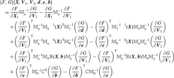 $$\begin{eqnarray}\displaystyle & & \displaystyle \{F,G\}[\boldsymbol{X},\boldsymbol{V}_{1},\boldsymbol{V}_{2},\boldsymbol{d},\boldsymbol{e},\boldsymbol{b}]\nonumber\\ \displaystyle & & \displaystyle \quad =\frac{\unicode[STIX]{x2202}F}{\unicode[STIX]{x2202}\boldsymbol{X}_{1}}\mathbb{M}_{p}^{-1}\frac{\unicode[STIX]{x2202}G}{\unicode[STIX]{x2202}\boldsymbol{V}_{1}}-\frac{\unicode[STIX]{x2202}G}{\unicode[STIX]{x2202}\boldsymbol{X}_{1}}\mathbb{M}_{p}^{-1}\frac{\unicode[STIX]{x2202}F}{\unicode[STIX]{x2202}\boldsymbol{V}_{1}}\nonumber\\ \displaystyle & & \displaystyle \qquad +\bigg(\frac{\unicode[STIX]{x2202}F}{\unicode[STIX]{x2202}\boldsymbol{V}_{1}}\bigg)^{\text{T}}\mathbb{M}_{p}^{-1}\mathbb{M}_{q}\unicode[STIX]{x1D726}^{1}(\boldsymbol{X})^{\text{T}}\mathbb{M}_{1}^{-1}\bigg(\frac{\unicode[STIX]{x2202}G}{\unicode[STIX]{x2202}\boldsymbol{d}}\bigg)-\bigg(\frac{\unicode[STIX]{x2202}F}{\unicode[STIX]{x2202}\boldsymbol{d}}\bigg)^{\text{T}}\mathbb{M}_{1}^{-1}\unicode[STIX]{x1D726}^{1}(\boldsymbol{X})\mathbb{M}_{q}\mathbb{M}_{p}^{-1}\bigg(\frac{\unicode[STIX]{x2202}G}{\unicode[STIX]{x2202}\boldsymbol{V}_{1}}\bigg)\nonumber\\ \displaystyle & & \displaystyle \qquad +\bigg(\frac{\unicode[STIX]{x2202}F}{\unicode[STIX]{x2202}\boldsymbol{V}_{2}}\bigg)^{\text{T}}\mathbb{M}_{p}^{-1}\mathbb{M}_{q}\unicode[STIX]{x1D726}^{0}(\boldsymbol{X})^{\text{T}}\mathbb{M}_{0}^{-1}\bigg(\frac{\unicode[STIX]{x2202}G}{\unicode[STIX]{x2202}\boldsymbol{e}}\bigg)-\bigg(\frac{\unicode[STIX]{x2202}F}{\unicode[STIX]{x2202}\boldsymbol{e}}\bigg)^{\text{T}}\mathbb{M}_{0}^{-1}\unicode[STIX]{x1D726}^{0}(\boldsymbol{X})\mathbb{M}_{q}\mathbb{M}_{p}^{-1}\bigg(\frac{\unicode[STIX]{x2202}G}{\unicode[STIX]{x2202}\boldsymbol{V}_{2}}\bigg)\nonumber\\ \displaystyle & & \displaystyle \qquad +\bigg(\frac{\unicode[STIX]{x2202}F}{\unicode[STIX]{x2202}\boldsymbol{V}_{1}}\bigg)^{\text{T}}\mathbb{M}_{p}^{-1}\mathbb{M}_{q}\mathbb{B}(\boldsymbol{X},\boldsymbol{b})\mathbb{M}_{p}^{-1}\bigg(\frac{\unicode[STIX]{x2202}G}{\unicode[STIX]{x2202}\boldsymbol{V}_{2}}\bigg)-\bigg(\frac{\unicode[STIX]{x2202}F}{\unicode[STIX]{x2202}\boldsymbol{V}_{2}}\bigg)^{\text{T}}\mathbb{M}_{p}^{-1}\mathbb{B}(\boldsymbol{X},\boldsymbol{b})\mathbb{M}_{q}\mathbb{M}_{p}^{-1}\bigg(\frac{\unicode[STIX]{x2202}G}{\unicode[STIX]{x2202}\boldsymbol{V}_{1}}\bigg)\nonumber\\ \displaystyle & & \displaystyle \qquad +\,\bigg(\frac{\unicode[STIX]{x2202}F}{\unicode[STIX]{x2202}\boldsymbol{e}}\bigg)^{\text{T}}\mathbb{M}_{0}^{-1}\mathbb{C}^{\text{T}}\bigg(\frac{\unicode[STIX]{x2202}G}{\unicode[STIX]{x2202}\boldsymbol{b}}\bigg)-\bigg(\frac{\unicode[STIX]{x2202}F}{\unicode[STIX]{x2202}\boldsymbol{b}}\bigg)^{\text{T}}\mathbb{C}\mathbb{M}_{0}^{-1}\bigg(\frac{\unicode[STIX]{x2202}G}{\unicode[STIX]{x2202}\boldsymbol{e}}\bigg).\end{eqnarray}$$
Here, we denote by
 $\mathbb{M}_{p}=\unicode[STIX]{x1D648}_{p}$
and
$\mathbb{M}_{p}=\unicode[STIX]{x1D648}_{p}$
and
 $\mathbb{M}_{q}=\unicode[STIX]{x1D648}_{q}$
the
$\mathbb{M}_{q}=\unicode[STIX]{x1D648}_{q}$
the
 $N_{p}\times N_{p}$
diagonal matrices holding the particle masses and charges, respectively. We denote by
$N_{p}\times N_{p}$
diagonal matrices holding the particle masses and charges, respectively. We denote by
 $\unicode[STIX]{x1D726}^{0}(\boldsymbol{X})$
the
$\unicode[STIX]{x1D726}^{0}(\boldsymbol{X})$
the
 $N_{p}\times N_{0}$
matrix with generic term
$N_{p}\times N_{0}$
matrix with generic term
 $\unicode[STIX]{x1D6EC}_{i}^{0}(\mathit{x}_{a})$
, where
$\unicode[STIX]{x1D6EC}_{i}^{0}(\mathit{x}_{a})$
, where
 $1\leqslant a\leqslant N_{p}$
and
$1\leqslant a\leqslant N_{p}$
and
 $1\leqslant i\leqslant N_{0}$
, and by
$1\leqslant i\leqslant N_{0}$
, and by
 $\unicode[STIX]{x1D726}^{1}(\boldsymbol{X})$
the
$\unicode[STIX]{x1D726}^{1}(\boldsymbol{X})$
the
 $N_{p}\times N_{1}$
matrix with generic term
$N_{p}\times N_{1}$
matrix with generic term
 $\unicode[STIX]{x1D6EC}_{i}^{1}(\mathit{x}_{a})$
, where
$\unicode[STIX]{x1D6EC}_{i}^{1}(\mathit{x}_{a})$
, where
 $1\leqslant a\leqslant N_{p}$
and
$1\leqslant a\leqslant N_{p}$
and
 $1\leqslant i\leqslant N_{1}$
. Further,
$1\leqslant i\leqslant N_{1}$
. Further,
 $\mathbb{B}(\boldsymbol{X},\boldsymbol{b})$
denotes the
$\mathbb{B}(\boldsymbol{X},\boldsymbol{b})$
denotes the
 $N_{p}\times N_{p}$
diagonal matrix with entries
$N_{p}\times N_{p}$
diagonal matrix with entries
 $$\begin{eqnarray}B_{h}(\mathit{x}_{a},t)=\mathop{\sum }_{i=1}^{N_{1}}b_{i}(t)\,\unicode[STIX]{x1D6EC}_{i}^{1}(\mathit{x}_{a}).\end{eqnarray}$$
The reduced bracket can be shown to satisfy the Jacobi identity by direct proof in full analogy to the proof for the full bracket shown in § 4.4. However, one can also follow along the lines of § 6.2 in order to arrive at the same result.
6.5 Discrete Hamiltonian and equations of motion
The discrete Hamiltonian is given in terms of the reduced set of degrees of freedom
 $\boldsymbol{u}=(\boldsymbol{X},\boldsymbol{V}_{1},\boldsymbol{V}_{2},\boldsymbol{d},\boldsymbol{e},\boldsymbol{b})$
by
$\boldsymbol{u}=(\boldsymbol{X},\boldsymbol{V}_{1},\boldsymbol{V}_{2},\boldsymbol{d},\boldsymbol{e},\boldsymbol{b})$
by
 $$\begin{eqnarray}H={\textstyle \frac{1}{2}}\,\boldsymbol{V}_{1}^{\text{T}}\mathbb{M}_{p}\boldsymbol{V}_{1}+{\textstyle \frac{1}{2}}\,\boldsymbol{V}_{2}^{\text{T}}\mathbb{M}_{p}\boldsymbol{V}_{2}+{\textstyle \frac{1}{2}}\,\boldsymbol{d}^{\text{T}}\mathbb{M}_{1}\boldsymbol{d}+{\textstyle \frac{1}{2}}\,\boldsymbol{e}^{\text{T}}\mathbb{M}_{0}\boldsymbol{e}+{\textstyle \frac{1}{2}}\,\boldsymbol{b}^{\text{T}}\mathbb{M}_{1}\boldsymbol{b}.\end{eqnarray}$$
and the equations of motion are obtained as
 $$\begin{eqnarray}\left.\begin{array}{@{}rcl@{}}\displaystyle \dot{\boldsymbol{X}}\ & =\ & \boldsymbol{V}_{1},\\ \displaystyle \dot{\boldsymbol{V}}_{1}\ & =\ & \mathbb{M}_{p}^{-1}\mathbb{M}_{q}(\unicode[STIX]{x1D726}^{1}(\boldsymbol{X})\boldsymbol{d}+\mathbb{B}(\boldsymbol{X},\boldsymbol{b})\boldsymbol{V}_{2}),\\ \displaystyle \dot{\boldsymbol{V}}_{2}\ & =\ & \mathbb{M}_{p}^{-1}\mathbb{M}_{q}(\unicode[STIX]{x1D726}^{0}(\boldsymbol{X})\boldsymbol{e}-\mathbb{B}(\boldsymbol{X},\boldsymbol{b})\boldsymbol{V}_{1}),\\ \displaystyle \dot{\boldsymbol{d}}\ & =\ & -\mathbb{M}_{1}^{-1}\unicode[STIX]{x1D726}^{1}(\boldsymbol{X})^{\text{T}}\mathbb{M}_{q}\boldsymbol{V}_{1},\\ \displaystyle \dot{\boldsymbol{e}}\ & =\ & \mathbb{M}_{0}^{-1}(\mathbb{C}^{\text{T}}\mathbb{M}_{1}\boldsymbol{b}(t)-\unicode[STIX]{x1D726}^{0}(\boldsymbol{X})^{\text{T}}\mathbb{M}_{q}\boldsymbol{V}_{2}),\\ \displaystyle \dot{\boldsymbol{b}}\ & =\ & -\mathbb{C}\boldsymbol{e}(t),\end{array}\right\}\end{eqnarray}$$
which is seen to be in direct correspondence with (6.3)–(6.7).
6.6 Hamiltonian splitting
The solution of the discrete equations of motion for
 $H_{D}+H_{E}$
at time
$H_{D}+H_{E}$
at time
 $\unicode[STIX]{x0394}t$
is
$\unicode[STIX]{x0394}t$
is
 $$\begin{eqnarray}\left.\begin{array}{@{}rcl@{}}\displaystyle \mathbb{M}_{p}\boldsymbol{V}_{1}(\unicode[STIX]{x0394}t)\ & =\ & \mathbb{M}_{p}\boldsymbol{V}_{1}(0)+\unicode[STIX]{x0394}t\,\mathbb{M}_{q}\unicode[STIX]{x1D726}^{1}(\boldsymbol{X}(0))\,\boldsymbol{d}(0),\\ \displaystyle \mathbb{M}_{p}\boldsymbol{V}_{2}(\unicode[STIX]{x0394}t)\ & =\ & \mathbb{M}_{p}\boldsymbol{V}_{2}(0)+\unicode[STIX]{x0394}t\,\mathbb{M}_{q}\unicode[STIX]{x1D726}^{0}(\boldsymbol{X}(0))\,\boldsymbol{e}(0),\\ \displaystyle \boldsymbol{b}(\unicode[STIX]{x0394}t)\ & =\ & \boldsymbol{b}(0)-\unicode[STIX]{x0394}t\,\mathbb{C}\boldsymbol{e}(0).\end{array}\right\}\end{eqnarray}$$
The solution of the discrete equations of motion for
 $H_{B}$
is
$H_{B}$
is
 $$\begin{eqnarray}\displaystyle \mathbb{M}_{0}\boldsymbol{e}(\unicode[STIX]{x0394}t)=\mathbb{M}_{0}\boldsymbol{e}(0)+\unicode[STIX]{x0394}t\,\mathbb{C}^{\text{T}}\mathbb{M}_{1}\boldsymbol{b}(0).\end{eqnarray}$$
The solution of the discrete equations of motion for
 $H_{p_{1}}$
is
$H_{p_{1}}$
is
 $$\begin{eqnarray}\left.\begin{array}{@{}rcl@{}}\displaystyle \boldsymbol{X}(\unicode[STIX]{x0394}t)\ & =\ & \boldsymbol{X}_{1}(0)+\unicode[STIX]{x0394}t\,\boldsymbol{V}_{1}(0),\\ \displaystyle \mathbb{M}_{p}\boldsymbol{V}_{2}(\unicode[STIX]{x0394}t)\ & =\ & \displaystyle \mathbb{M}_{p}\boldsymbol{V}_{2}(0)-\!\int _{0}^{\unicode[STIX]{x0394}t}\mathbb{M}_{q}\mathbb{B}(\boldsymbol{X}(t),\boldsymbol{b}(0))\boldsymbol{V}_{1}(0)\,\text{d}t,\\ \displaystyle \mathbb{M}_{1}\boldsymbol{d}(\unicode[STIX]{x0394}t)\ & =\ & \displaystyle \mathbb{M}_{1}\boldsymbol{d}(0)-\!\int _{0}^{\unicode[STIX]{x0394}t}\unicode[STIX]{x1D726}^{1}(\boldsymbol{X}(t))^{\text{T}}\mathbb{M}_{q}\boldsymbol{V}_{1}(0)\,\text{d}t,\end{array}\right\}\end{eqnarray}$$
and for
 $H_{p_{2}}$
it is
$H_{p_{2}}$
it is
 $$\begin{eqnarray}\left.\begin{array}{@{}rcl@{}}\displaystyle \mathbb{M}_{p}\boldsymbol{V}_{1}(\unicode[STIX]{x0394}t)\ & =\ & \displaystyle \mathbb{M}_{p}\boldsymbol{V}_{1}(0)+\int _{0}^{\unicode[STIX]{x0394}t}\mathbb{M}_{q}\mathbb{B}(\boldsymbol{X}(0),\boldsymbol{b}(0))\boldsymbol{V}_{2}(0)\,\text{d}t,\\ \displaystyle \mathbb{M}_{0}\boldsymbol{e}(\unicode[STIX]{x0394}t)\ & =\ & \displaystyle \mathbb{M}_{0}\boldsymbol{e}(0)-\!\int _{0}^{\unicode[STIX]{x0394}t}\unicode[STIX]{x1D726}^{1}(\boldsymbol{X}(0))^{\text{T}}\mathbb{M}_{q}\boldsymbol{V}_{2}(0)\,\text{d}t,\end{array}\right\}\end{eqnarray}$$
respectively.
7 Numerical experiments
We have implemented the Hamiltonian splitting scheme as well as the Boris–Yee scheme from appendix A as part of the SeLaLib library (http://selalib.gforge.inria.fr/). In this section, we present results for various test cases in 1d2v, comparing the conservation properties of the total energy and of the Casimirs for the two schemes. We simulate the electron distribution function in a neutralizing ion background. In all experiments, we have used splines of order three for the 0-forms. The particle loading was done using Sobol numbers and antithetic sampling (symmetric around the middle of the domain in
 $x$
and around the mean value of the Gaussian from which we are sampling in each velocity dimension). We sample uniformly in
$x$
and around the mean value of the Gaussian from which we are sampling in each velocity dimension). We sample uniformly in
 $x$
and from the Gaussians of the initial distribution in each velocity dimension.
$x$
and from the Gaussians of the initial distribution in each velocity dimension.
7.1 Weibel instability
We consider the Weibel instability studied in Weibel (Reference Weibel1959) in the form simulated in Crouseilles et al. (Reference Crouseilles, Einkemmer and Faou2015). We study a reduced 1d2v model with a perturbation along
 $x_{1}$
, a magnetic field along
$x_{1}$
, a magnetic field along
 $x_{3}$
and electric fields along the
$x_{3}$
and electric fields along the
 $x_{1}$
and
$x_{1}$
and
 $x_{2}$
directions. Moreover, we assume that the distribution function is independent of
$x_{2}$
directions. Moreover, we assume that the distribution function is independent of
 $v_{3}$
. The initial distribution and fields are of the form
$v_{3}$
. The initial distribution and fields are of the form
 $$\begin{eqnarray}\displaystyle & \displaystyle f(x,\boldsymbol{v},t=0)=\frac{1}{2\unicode[STIX]{x03C0}\unicode[STIX]{x1D70E}_{1}\unicode[STIX]{x1D70E}_{2}}\exp \left(-\frac{1}{2}\left(\frac{v_{1}^{2}}{\unicode[STIX]{x1D70E}_{1}^{2}}+\frac{v_{2}^{2}}{\unicode[STIX]{x1D70E}_{2}^{2}}\right)\right)\left(1+\unicode[STIX]{x1D6FC}\cos (kx)\right),\quad x\in [0,2\unicode[STIX]{x03C0}/k), & \displaystyle \nonumber\\ \displaystyle & & \displaystyle\end{eqnarray}$$
 $$\begin{eqnarray}\displaystyle & \displaystyle B_{3}(x,t=0)=\unicode[STIX]{x1D6FD}\cos (kx), & \displaystyle\end{eqnarray}$$
 $$\begin{eqnarray}\displaystyle & \displaystyle E_{2}(x,t=0)=0, & \displaystyle\end{eqnarray}$$
and
 $E_{1}(x,t=0)$
is computed from Poisson’s equation. In our simulations, we use the following choice of parameters,
$E_{1}(x,t=0)$
is computed from Poisson’s equation. In our simulations, we use the following choice of parameters,
 $\unicode[STIX]{x1D70E}_{1}=0.02/\sqrt{2}$
,
$\unicode[STIX]{x1D70E}_{1}=0.02/\sqrt{2}$
,
 $\unicode[STIX]{x1D70E}_{2}=\sqrt{12}\unicode[STIX]{x1D70E}_{1}$
,
$\unicode[STIX]{x1D70E}_{2}=\sqrt{12}\unicode[STIX]{x1D70E}_{1}$
,
 $k=1.25$
,
$k=1.25$
,
 $\unicode[STIX]{x1D6FC}=0$
and
$\unicode[STIX]{x1D6FC}=0$
and
 $\unicode[STIX]{x1D6FD}=-10^{-4}$
. Note that these are the same parameters as in Crouseilles et al. (Reference Crouseilles, Einkemmer and Faou2015) except for the fact that we sample from the Maxwellian without perturbation in
$\unicode[STIX]{x1D6FD}=-10^{-4}$
. Note that these are the same parameters as in Crouseilles et al. (Reference Crouseilles, Einkemmer and Faou2015) except for the fact that we sample from the Maxwellian without perturbation in
 $x_{1}$
.
$x_{1}$
.
The dispersion relation from Weibel (Reference Weibel1959) applied to our model reads
 $$\begin{eqnarray}D(\unicode[STIX]{x1D714},k)=\unicode[STIX]{x1D714}^{2}-k^{2}+\left(\frac{\unicode[STIX]{x1D70E}_{2}}{\unicode[STIX]{x1D70E}_{1}}\right)^{2}-1-\left(\frac{\unicode[STIX]{x1D70E}_{2}}{\unicode[STIX]{x1D70E}_{1}}\right)^{2}\unicode[STIX]{x1D719}\left(\frac{\unicode[STIX]{x1D714}}{\unicode[STIX]{x1D70E}_{1}k}\right)\frac{\unicode[STIX]{x1D714}}{\unicode[STIX]{x1D70E}_{1}k},\end{eqnarray}$$
where
 $\unicode[STIX]{x1D719}(z)=\exp (-1/2z^{2})\int _{-\text{i}\infty }^{z}\exp (1/2\unicode[STIX]{x1D709}^{2})\,\text{d}\unicode[STIX]{x1D709}$
. For our parameter choice, this gives a growth rate of 0.02784. In figure 1, we show the electric and magnetic energies together with the analytic growth rate. We see that the growth rate is verified in the numerical solution. This simulation was performed with 100 000 particles, 32 grid points, splines of degree 3 and 2 and
$\unicode[STIX]{x1D719}(z)=\exp (-1/2z^{2})\int _{-\text{i}\infty }^{z}\exp (1/2\unicode[STIX]{x1D709}^{2})\,\text{d}\unicode[STIX]{x1D709}$
. For our parameter choice, this gives a growth rate of 0.02784. In figure 1, we show the electric and magnetic energies together with the analytic growth rate. We see that the growth rate is verified in the numerical solution. This simulation was performed with 100 000 particles, 32 grid points, splines of degree 3 and 2 and
 $\unicode[STIX]{x0394}t=0.05$
. Note that we have chosen a very large number of particles in order to obtain a solution of very high quality. In practice, the Weibel instability can also be simulated with much fewer particles (cf. § 7.5).
$\unicode[STIX]{x0394}t=0.05$
. Note that we have chosen a very large number of particles in order to obtain a solution of very high quality. In practice, the Weibel instability can also be simulated with much fewer particles (cf. § 7.5).
In table 1, we show the conservation properties of our splitting with various orders of the splitting (cf. § 5.2) and compare them also to the Boris–Yee scheme. The other numerical parameters are kept as before.
We can see that Gauss’ law is satisfied in each time step for the Hamiltonian splitting. This is a Casimir (cf. § 2.2) and therefore naturally conserved by the Hamiltonian splitting. On the other hand, this is not the case for the Boris–Yee scheme.
We can also see that the energy error improves with the order of the splitting; however, the Hamiltonian splitting method as well as the Boris–Yee scheme are not energy conserving. The time evolution of the total energy error is depicted in figure 2 for the various methods.

Figure 1. Weibel instability: the two electric and the magnetic energies together with the analytic growth rate.

Figure 2. Weibel instability: difference of total energy and its initial value as a function of time for various integrators.
Table 1. Weibel instability: maximum error in the total energy and Gauss’ law until time 500 for simulation with various integrators: Lie–Trotter splitting from (5.17) (Lie), Strang splitting from (5.18) (Strang), second-order splitting with 4 Lie parts defined in (5.22) (2nd, 4 Lie), fourth-order splitting with 3 Strang parts defined in (5.23) (4th, 3 Strang) and 10 Lie parts defined in (5.25) (4th, 10 Lie).
7.2 Streaming Weibel instability
As a second test case, we consider the streaming Weibel instability. We study the same reduced model as in the previous section, but following Califano, Pegoraro & Bulanov (Reference Califano, Pegoraro and Bulanov1997), Cheng et al. (Reference Cheng, Gamba, Li and Morrison2014c ) the initial distribution and fields are prescribed as
 $$\begin{eqnarray}\displaystyle f(x,\boldsymbol{v},t=0) & = & \displaystyle \frac{1}{2\unicode[STIX]{x03C0}\unicode[STIX]{x1D70E}^{2}}\exp \bigg(-\frac{v_{1}^{2}}{2\unicode[STIX]{x1D70E}^{2}}\bigg)\bigg(\unicode[STIX]{x1D6FF}\exp \bigg(-\frac{(v_{2}-v_{0,1})^{2}}{2\unicode[STIX]{x1D70E}^{2}}\bigg)\nonumber\\ \displaystyle & & \displaystyle +\,(1-\unicode[STIX]{x1D6FF})\exp \bigg(-\frac{(v_{2}-v_{0,2})^{2}}{2\unicode[STIX]{x1D70E}^{2}}\bigg)\bigg),\end{eqnarray}$$
 $$\begin{eqnarray}\displaystyle B_{3}(x,t=0) & = & \displaystyle \unicode[STIX]{x1D6FD}\sin (kx),\end{eqnarray}$$
 $$\begin{eqnarray}\displaystyle E_{2}(x,t=0) & = & \displaystyle 0,\end{eqnarray}$$
and
 $E_{1}(x,t=0)$
is computed from Poisson’s equation.
$E_{1}(x,t=0)$
is computed from Poisson’s equation.
We set the parameters to the following values
 $\unicode[STIX]{x1D70E}=0.1/\sqrt{2}$
,
$\unicode[STIX]{x1D70E}=0.1/\sqrt{2}$
,
 $k=0.2$
,
$k=0.2$
,
 $\unicode[STIX]{x1D6FD}=-10^{-3}$
,
$\unicode[STIX]{x1D6FD}=-10^{-3}$
,
 $v_{0,1}=0.5$
,
$v_{0,1}=0.5$
,
 $v_{0,2}=-0.1$
and
$v_{0,2}=-0.1$
and
 $\unicode[STIX]{x1D6FF}=1/6$
. The parameters are chosen as in the case 2 of Cheng et al. (Reference Cheng, Gamba, Li and Morrison2014c
). The growth rate of energy of the second component of the electric field was determined to be 0.03 in Califano et al. (Reference Califano, Pegoraro and Bulanov1997). In figure 3, we show the electric and magnetic energies together with the analytic growth rate. We see that the growth rate is verified in the numerical solution. This simulation was performed on the domain
$\unicode[STIX]{x1D6FF}=1/6$
. The parameters are chosen as in the case 2 of Cheng et al. (Reference Cheng, Gamba, Li and Morrison2014c
). The growth rate of energy of the second component of the electric field was determined to be 0.03 in Califano et al. (Reference Califano, Pegoraro and Bulanov1997). In figure 3, we show the electric and magnetic energies together with the analytic growth rate. We see that the growth rate is verified in the numerical solution. This simulation was performed on the domain
 $x\in [0,2\unicode[STIX]{x03C0}/k)$
with 20 000 000 particles, 128 grid points, splines of degree 3 and 2 and
$x\in [0,2\unicode[STIX]{x03C0}/k)$
with 20 000 000 particles, 128 grid points, splines of degree 3 and 2 and
 $\unicode[STIX]{x0394}t=0.01$
. Observe that the energy of the
$\unicode[STIX]{x0394}t=0.01$
. Observe that the energy of the
 $E_{1}$
component of the electric field starts to increase at times earlier than in Califano et al. (Reference Califano, Pegoraro and Bulanov1997), which is caused by particle noise.
$E_{1}$
component of the electric field starts to increase at times earlier than in Califano et al. (Reference Califano, Pegoraro and Bulanov1997), which is caused by particle noise.
As for the Weibel instability, we compare the conservation properties in table 2 for various integrators. Again we see that the Hamiltonian splitting conserves Gauss’ law as opposed to the Boris–Yee scheme. The energy conservation properties of the various schemes show approximately the same behaviour as in the previous test case (see also figure 4 for the time evolution of the energy error).
Table 2. Streaming Weibel instability: maximum error in the total energy and Gauss’ law until time 200 for simulation with various integrators.


Figure 3. Streaming Weibel instability: the two electric and the magnetic energies together with the analytic growth rate.

Figure 4. Streaming Weibel instability: difference of total energy and its initial value as a function of time for various integrators.
7.3 Strong Landau damping
Table 3. Damping and growth rates for strong Landau damping.
Finally, we also study the electrostatic example of strong Landau damping with initial distribution
 $$\begin{eqnarray}f(x,\boldsymbol{v})=\exp \frac{1}{2\unicode[STIX]{x03C0}\unicode[STIX]{x1D70E}^{2}}\left(-\frac{v_{1}^{2}+v_{2}^{2}}{2\unicode[STIX]{x1D70E}^{2}}\right)\,(1+\unicode[STIX]{x1D6FC}\,\cos (kx)),\quad x\in [0,2\unicode[STIX]{x03C0}/k),\boldsymbol{v}\in \mathbb{R}^{2}.\end{eqnarray}$$
The physical parameters are chosen as
 $\unicode[STIX]{x1D70E}=1$
,
$\unicode[STIX]{x1D70E}=1$
,
 $k=0.5$
,
$k=0.5$
,
 $\unicode[STIX]{x1D6FC}=0.5$
and the numerical parameters as
$\unicode[STIX]{x1D6FC}=0.5$
and the numerical parameters as
 $\unicode[STIX]{x1D6E5}t=0.05$
,
$\unicode[STIX]{x1D6E5}t=0.05$
,
 $n_{x}=32$
and 100 000 particles. The fields
$n_{x}=32$
and 100 000 particles. The fields
 $B_{3}$
and
$B_{3}$
and
 $E_{2}$
are initialized to zero and remain zero over time. In this example, we essentially solve the Vlasov–Ampère equation with results equivalent to the Vlasov–Poisson equations. In figure 5 we show the time evolution of the electric energy associated with
$E_{2}$
are initialized to zero and remain zero over time. In this example, we essentially solve the Vlasov–Ampère equation with results equivalent to the Vlasov–Poisson equations. In figure 5 we show the time evolution of the electric energy associated with
 $E_{1}$
. We have also fitted a damping and growth rate (using the marked local maxima in the plot). These are in good agreement with other codes (see table 3). Again the energy conservation for the various method is visualized as a function of time in figure 6. And again we see that the fourth-order methods give excellent energy conservation.
$E_{1}$
. We have also fitted a damping and growth rate (using the marked local maxima in the plot). These are in good agreement with other codes (see table 3). Again the energy conservation for the various method is visualized as a function of time in figure 6. And again we see that the fourth-order methods give excellent energy conservation.

Figure 5. Landau damping: electric energy with fitted damping and growth rates.

Figure 6. Landau damping: total energy error.
7.4 Backward error analysis
For the Lie–Trotter splitting, the error in the Hamiltonian
 $H$
is of order
$H$
is of order
 $\unicode[STIX]{x0394}t$
. However, using backward error analysis (cf. § 5.3), modified Hamiltonians can be computed, which are preserved to higher order. Accounting for first-order corrections
$\unicode[STIX]{x0394}t$
. However, using backward error analysis (cf. § 5.3), modified Hamiltonians can be computed, which are preserved to higher order. Accounting for first-order corrections
 $\tilde{H}_{1}$
, the error in the modified Hamiltonian,
$\tilde{H}_{1}$
, the error in the modified Hamiltonian,
 $$\begin{eqnarray}\tilde{H}=H+\unicode[STIX]{x0394}t\tilde{H}_{1}+O(\unicode[STIX]{x0394}t^{2}),\end{eqnarray}$$
is of order
 $(\unicode[STIX]{x0394}t)^{2}$
. For the 1d2v example, this correction is obtained as
$(\unicode[STIX]{x0394}t)^{2}$
. For the 1d2v example, this correction is obtained as
 $$\begin{eqnarray}\tilde{H}_{1}={\textstyle \frac{1}{2}}[\{H_{D}+H_{E},H_{B}\}+\{H_{p_{1}},H_{p_{2}}\}+\{H_{D}+H_{E}+H_{B},H_{p_{1}}+H_{p_{2}}\}],\end{eqnarray}$$
with the various Poisson brackets computed as
 $$\begin{eqnarray}\left.\begin{array}{@{}rcl@{}}\displaystyle \{H_{D},H_{B}\}\ & =\ & 0,\\ \displaystyle \{H_{E},H_{B}\}\ & =\ & \boldsymbol{e}^{\text{T}}\mathbb{C}^{\text{T}}\boldsymbol{b},\\ \displaystyle \{H_{p_{1}},H_{p_{2}}\}\ & =\ & \boldsymbol{V}_{1}\unicode[STIX]{x1D648}_{q}\mathbb{B}(\boldsymbol{b},\boldsymbol{X})^{\text{T}}\,\boldsymbol{V}_{2},\\ \displaystyle \{H_{D},H_{p_{1}}\}\ & =\ & -\boldsymbol{d}^{\text{T}}\unicode[STIX]{x1D726}^{1}(\boldsymbol{X})^{\text{T}}\unicode[STIX]{x1D648}_{q}\boldsymbol{V}_{1},\\ \displaystyle \{H_{D},H_{p_{2}}\}\ & =\ & 0,\\ \displaystyle \{H_{E},H_{p_{1}}\}\ & =\ & 0,\\ \displaystyle \{H_{E},H_{p_{2}}\}\ & =\ & -\boldsymbol{e}^{\text{T}}\unicode[STIX]{x1D726}^{0}(\boldsymbol{X})^{\text{T}}\unicode[STIX]{x1D648}_{q}\boldsymbol{V}_{2},\\ \displaystyle \{H_{B},H_{p_{1}}\}\ & =\ & 0,\\ \displaystyle \{H_{B},H_{p_{2}}\}\ & =\ & 0.\end{array}\right\}\end{eqnarray}$$
In figure 7, we show the maximum and
 $\ell _{2}$
error of the energy and the corrected energy for the Weibel instability test case with the parameters in § 7.1. The simulations were performed with 100 000 particles, 32 grid points, splines of degree 3 and 2 and
$\ell _{2}$
error of the energy and the corrected energy for the Weibel instability test case with the parameters in § 7.1. The simulations were performed with 100 000 particles, 32 grid points, splines of degree 3 and 2 and
 $\unicode[STIX]{x0394}t=0.01,0.02,0.05$
. We can see that the theoretical convergence rates are verified in the numerical experiments. Figure 8 shows the energy as well as the modified energy for the Weibel instability test case simulated with a time step of
$\unicode[STIX]{x0394}t=0.01,0.02,0.05$
. We can see that the theoretical convergence rates are verified in the numerical experiments. Figure 8 shows the energy as well as the modified energy for the Weibel instability test case simulated with a time step of
 $0.05$
.
$0.05$
.

Figure 7. Weibel instability: error (maximum norm and
 $\ell _{2}$
norm) in the total energy for simulations with
$\ell _{2}$
norm) in the total energy for simulations with
 $\unicode[STIX]{x0394}t=0.01,0.02,0.05$
.
$\unicode[STIX]{x0394}t=0.01,0.02,0.05$
.

Figure 8. Weibel instability: energy and first-order corrected energy for simulation with
 $\unicode[STIX]{x0394}t=0.05$
.
$\unicode[STIX]{x0394}t=0.05$
.
7.5 Momentum conservation
Finally, let us discuss conservation of momentum for our one species 1d2v equations. In this case, equation (2.30) becomes
 $$\begin{eqnarray}\frac{\text{d}P_{e,1,2}}{\,\text{d}t}=-\!\int E_{1,2}(x,t)\,\text{d}x.\end{eqnarray}$$
For
 $P_{e,1}(t)$
from (6.4) we get
$P_{e,1}(t)$
from (6.4) we get
 $$\begin{eqnarray}\frac{\text{d}}{\text{d}t}\int E_{1}(x,t)\,\text{d}x=-\!\int j_{1}(x,t)\,\text{d}x.\end{eqnarray}$$
Since in general
 $\int j_{1}(x,t)\,\text{d}x\neq 0$
, momentum is not conserved. As a means of testing momentum conservation, Crouseilles et al. (Reference Crouseilles, Einkemmer and Faou2015) replaced (6.4) by
$\int j_{1}(x,t)\,\text{d}x\neq 0$
, momentum is not conserved. As a means of testing momentum conservation, Crouseilles et al. (Reference Crouseilles, Einkemmer and Faou2015) replaced (6.4) by
 $$\begin{eqnarray}\frac{\unicode[STIX]{x2202}E_{1}(x,t)}{\unicode[STIX]{x2202}t}=-j_{1}(x,t)+\int j_{1}(x,t)\,\text{d}x.\end{eqnarray}$$
Thus, for this artificial dynamics, momentum will be conserved if
 $\int E_{1}(x,0)\,\text{d}x=0$
. Instead, we do not modify the equations but check the validity of (7.12). We define a discrete version of (7.12), integrated over time, in the following way:
$\int E_{1}(x,0)\,\text{d}x=0$
. Instead, we do not modify the equations but check the validity of (7.12). We define a discrete version of (7.12), integrated over time, in the following way:
 $$\begin{eqnarray}\displaystyle \tilde{P}_{e,1}^{n} & = & \displaystyle P_{e,1}^{0}-\frac{\unicode[STIX]{x0394}t}{2}\mathop{\sum }_{m=1}^{n}\left(\int D_{h}^{m-1}(x)\,\text{d}x+\int D_{h}^{m}(x)\,\text{d}x\right),\end{eqnarray}$$
 $$\begin{eqnarray}\displaystyle \tilde{P}_{e,2}^{n} & = & \displaystyle P_{e,2}^{0}-\frac{\unicode[STIX]{x0394}t}{2}\mathop{\sum }_{m=1}^{n}\left(\int E_{h}^{m-1}(x)\,\text{d}x+\int E_{h}^{m}(x)\,\text{d}x\right).\end{eqnarray}$$
Our numerical scheme does not conserve momentum exactly. However, the error in momentum can be kept rather small during the linear phase of the simulation. Note that in all our examples,
 $\int j_{1,2}(x,t)\,\text{d}x=0$
. For a Gaussian initial distribution, the antithetic sampling ensures that
$\int j_{1,2}(x,t)\,\text{d}x=0$
. For a Gaussian initial distribution, the antithetic sampling ensures that
 $\int j_{1,2}(x,t)\,\text{d}x=0$
holds in the discrete sense. Figure 9 shows the momentum error in a simulation of the Weibel instability as considered in § 7.1, but up to time 2000 and with 25 600 particles sampled from pseudo-random numbers and Sobol numbers, for both plain and antithetical sampling. For the plain sampling, momentum error is a bit smaller for Sobol numbers compared to pseudo-random numbers during the linear phase. For the antithetic sampling, we can see that the momentum error is very small until time 200 (linear phase). However, when nonlinear effects start to dominate, the momentum error slowly increases until it has reached the same level as the momentum error for plain Sobol number sampling. The level depends on the number of particles (cf. table 4). Note that the sampling does not seem to have an influence on the energy conservation as can be seen in figure 10 that compares the energy error for the various sampling techniques. The curves show that the energy error is related to the increase in potential energy during the linear phase but does not further grow during the nonlinear phase.
$\int j_{1,2}(x,t)\,\text{d}x=0$
holds in the discrete sense. Figure 9 shows the momentum error in a simulation of the Weibel instability as considered in § 7.1, but up to time 2000 and with 25 600 particles sampled from pseudo-random numbers and Sobol numbers, for both plain and antithetical sampling. For the plain sampling, momentum error is a bit smaller for Sobol numbers compared to pseudo-random numbers during the linear phase. For the antithetic sampling, we can see that the momentum error is very small until time 200 (linear phase). However, when nonlinear effects start to dominate, the momentum error slowly increases until it has reached the same level as the momentum error for plain Sobol number sampling. The level depends on the number of particles (cf. table 4). Note that the sampling does not seem to have an influence on the energy conservation as can be seen in figure 10 that compares the energy error for the various sampling techniques. The curves show that the energy error is related to the increase in potential energy during the linear phase but does not further grow during the nonlinear phase.

Figure 9. Weibel instability: error in the first component of the momentum for plain and antithetic Sobol sampling.
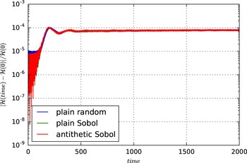
Figure 10. Weibel instability: total energy error for plain and antithetic Sobol sampling.
Table 4. Weibel instability: maximum error in both components of the momentum for simulations until time 2000 with various numbers of particles and 32 grid cells.
For the streaming Weibel instability on the other hand, we have a sum of two Gaussians in the second component of the velocity. Since in our sampling method we draw the particles based on Sobol quasi-random numbers, the fractions drawn from each of the Gaussians are not exactly given by
 $\unicode[STIX]{x1D6FF}$
and
$\unicode[STIX]{x1D6FF}$
and
 $1-\unicode[STIX]{x1D6FF}$
as in (7.5). Hence
$1-\unicode[STIX]{x1D6FF}$
as in (7.5). Hence
 $\int j_{2}(x,t)\,\text{d}x$
is small but non-zero. Comparing the discrete momentum defined by (7.16) with the discretization of its definition (2.25),
$\int j_{2}(x,t)\,\text{d}x$
is small but non-zero. Comparing the discrete momentum defined by (7.16) with the discretization of its definition (2.25),
 $$\begin{eqnarray}P_{e,2}^{n}=\mathop{\sum }_{a}v_{a,2}^{n}m_{a}w_{a}-\!\int D_{h}^{n}(x)B_{h}^{n}(x)\,\text{d}x,\end{eqnarray}$$
we see a maximum deviation over time of
 $1.6\times 10^{-16}$
for a simulation with Strang splitting,
$1.6\times 10^{-16}$
for a simulation with Strang splitting,
 $20\,000\,000$
particles, 128 grid points and
$20\,000\,000$
particles, 128 grid points and
 $\unicode[STIX]{x0394}t=0.01$
. This shows that our discretization with a Strang splitting conserves (7.12) in the sense of (7.16) to very high accuracy.
$\unicode[STIX]{x0394}t=0.01$
. This shows that our discretization with a Strang splitting conserves (7.12) in the sense of (7.16) to very high accuracy.
8 Summary
In this work, a general framework for geometric finite element particle-in-cell methods for the Vlasov–Maxwell system was presented. The discretization proceeded in two steps. First, a semi-discretization of the noncanonical Poisson bracket was obtained, which preserves the Jacobi identity and important Casimir invariants, so that the resulting finite-dimensional system is still Hamiltonian. Then, the system was discretized in time by Hamiltonian splitting methods, still retaining exact conservation of Casimirs, which in practice means exact conservation of Gauss’ law and
 $\text{div}\,B=0$
. Therefore the resulting method corresponds to one of the rare instances of a genuine Poisson integrator. Energy is not preserved exactly, but backward error analysis showed that the energy error does not depend on the degrees of freedom, the number of particles or the number of time steps. The favourable properties of the method were verified in various numerical experiments in 1d2v using splines as basis functions for the electromagnetic fields. One of the advantages of our approach is that conservation laws such as those for energy and charge are not manufactured into the scheme ‘by hand’ but follow automatically from preserving the underlying geometric structure of the equations.
$\text{div}\,B=0$
. Therefore the resulting method corresponds to one of the rare instances of a genuine Poisson integrator. Energy is not preserved exactly, but backward error analysis showed that the energy error does not depend on the degrees of freedom, the number of particles or the number of time steps. The favourable properties of the method were verified in various numerical experiments in 1d2v using splines as basis functions for the electromagnetic fields. One of the advantages of our approach is that conservation laws such as those for energy and charge are not manufactured into the scheme ‘by hand’ but follow automatically from preserving the underlying geometric structure of the equations.
The basic structure and implementation strategy of the code is very similar to existing finite element particle-in-cell methods for the Vlasov–Maxwell system. The main difference is the use of basis functions of mixed polynomial degree for the electromagnetic fields. The particle pusher is very similar to usual schemes, such as the Boris scheme, the only additional complexity being the exact computation of some line integrals. The cost of the method is comparable to existing charge-conserving algorithms like the method of Villasenor & Buneman or the Boris correction method. It is somewhat more expensive than non-charge-conserving methods, but such schemes are known to be prone to spurious instabilities that can lead to unphysical simulation results. Even though only examples in 1d2v were shown, there are no conceptional differences or difficulties when going from one to two or to three spatial dimensions. The building blocks of the code are identical in all three cases due to the tensor-product structure of the Eulerian grid and the splitting in time. Details on the implementation of a three-dimensional version of the code as well as a comparison with existing methods will be disseminated in a subsequent publication.
The generality of the framework opens up several new paths for subsequent research. Instead of splines, other finite element spaces that form a deRham complex could be used, e.g. mimetic spectral elements or Nédélec elements for 1-forms and Raviart–Thomas elements for two-forms. Further, it also should be possible to apply this approach to other systems like the gyrokinetic Vlasov–Maxwell system (Burby et al. Reference Burby, Brizard, Morrison and Qin2015; Burby Reference Burby2017), although in this case the necessity for new splitting schemes or other time integration strategies might arise. Energy-preserving time stepping methods might provide an alternative to Hamiltonian splitting algorithms, where a suitable splitting cannot be easily found. This is a topic currently under investigation. So is the treatment of the relativistic Vlasov–Maxwell system, which follows very closely along the lines of the non-relativistic system. This is a problem of interest in its own right, featuring an even larger set of invariants one should attempt to preserve in the discretization. Another extension of the GEMPIC framework under development is the inclusion of non-ideal, non-Hamiltonian effects, most importantly collisions. An appropriate geometric description for such effects can be provided either microscopically by stochastic Hamiltonian processes or macroscopically by metriplectic brackets (Morrison Reference Morrison1986).
Acknowledgements
Useful discussions with Omar Maj and Marco Restelli are gratefully appreciated. M.K. has received funding from the European Union’s Horizon 2020 research and innovation programme under the Marie Sklodowska-Curie grant agreement No 708124. P.J.M. received support from the US Dept. of Energy Contract #DE-FG05-80ET-53088 and a Forschungspreis from the Humboldt Foundation. This work has been carried out within the framework of the EUROfusion Consortium and has received funding from the Euratom research and training programme 2014-2018 under grant agreement no. 633053. The views and opinions expressed herein do not necessarily reflect those of the European Commission. A part of this work was carried out using the HELIOS supercomputer system at Computational Simulation Centre of International Fusion Energy Research Centre (IFERC-CSC), Aomori, Japan, under the Broader Approach collaboration between Euratom and Japan, implemented by Fusion for Energy and QST.
Appendix A. The Boris–Yee scheme
As an alternative discretization scheme, we consider a Boris–Yee scheme (Yee Reference Yee1966; Boris Reference Boris1970) with our conforming finite elements. The scheme uses a time staggering working with the variables
 $\boldsymbol{X}^{n+1/2}=\boldsymbol{X}(t^{n}+\unicode[STIX]{x0394}t/2)$
,
$\boldsymbol{X}^{n+1/2}=\boldsymbol{X}(t^{n}+\unicode[STIX]{x0394}t/2)$
,
 $\boldsymbol{d}^{n+1/2}=\boldsymbol{d}(t^{n}+\unicode[STIX]{x0394}t/2)$
,
$\boldsymbol{d}^{n+1/2}=\boldsymbol{d}(t^{n}+\unicode[STIX]{x0394}t/2)$
,
 $\boldsymbol{e}^{n+1/2}=\boldsymbol{e}(t^{n}+\unicode[STIX]{x0394}t/2)$
,
$\boldsymbol{e}^{n+1/2}=\boldsymbol{e}(t^{n}+\unicode[STIX]{x0394}t/2)$
,
 $\boldsymbol{V}^{n}=\boldsymbol{V}(t^{n})$
, and
$\boldsymbol{V}^{n}=\boldsymbol{V}(t^{n})$
, and
 $\boldsymbol{b}^{n}=\boldsymbol{b}(t^{n})$
in the
$\boldsymbol{b}^{n}=\boldsymbol{b}(t^{n})$
in the
 $n$
th time step
$n$
th time step
 $t^{n}=t^{0}+n\unicode[STIX]{x0394}t$
. The Hamiltonian at time
$t^{n}=t^{0}+n\unicode[STIX]{x0394}t$
. The Hamiltonian at time
 $t^{n}$
is defined as
$t^{n}$
is defined as
 $$\begin{eqnarray}\displaystyle H & = & \displaystyle {\textstyle \frac{1}{2}}\,(\boldsymbol{V}_{1}^{n})^{\text{T}}\unicode[STIX]{x1D648}_{p}\boldsymbol{V}_{1}^{n}+{\textstyle \frac{1}{2}}\,(\boldsymbol{V}_{2}^{n})^{\text{T}}\unicode[STIX]{x1D648}_{p}\boldsymbol{V}_{2}^{n}+{\textstyle \frac{1}{2}}\,(\boldsymbol{d}^{n-1/2})^{\text{T}}\mathbb{M}_{1}\boldsymbol{d}^{n+1/2}\nonumber\\ \displaystyle & & \displaystyle +\,{\textstyle \frac{1}{2}}\,(\boldsymbol{e}^{n-1/2})^{\text{T}}\mathbb{M}_{0}\boldsymbol{e}^{n+1/2}+{\textstyle \frac{1}{2}}\,(\boldsymbol{b}^{n})^{\text{T}}\mathbb{M}_{1}\boldsymbol{b}^{n}.\end{eqnarray}$$
Given
 $\boldsymbol{X}^{n-1/2}$
,
$\boldsymbol{X}^{n-1/2}$
,
 $\boldsymbol{d}^{n-1/2}$
,
$\boldsymbol{d}^{n-1/2}$
,
 $\boldsymbol{e}^{n-1/2}$
,
$\boldsymbol{e}^{n-1/2}$
,
 $\boldsymbol{V}^{n-1}$
,
$\boldsymbol{V}^{n-1}$
,
 $\boldsymbol{b}^{n-1}$
the Vlasov–Maxwell system is propagated by the following time step:
$\boldsymbol{b}^{n-1}$
the Vlasov–Maxwell system is propagated by the following time step:
-
(i) Compute
 $\boldsymbol{b}^{n}$
according to (A 2)and
$$\begin{eqnarray}b_{i}^{n}=b_{i}^{n-1}-\frac{\unicode[STIX]{x0394}t}{\unicode[STIX]{x0394}x}\left(e_{i}^{n-1/2}-e_{i-1}^{n-1/2}\right).\end{eqnarray}$$
$\boldsymbol{b}^{n-1/2}=(\boldsymbol{b}^{n-1}+\boldsymbol{b}^{n})/2$
.
$\boldsymbol{b}^{n}$
according to (A 2)and
$$\begin{eqnarray}b_{i}^{n}=b_{i}^{n-1}-\frac{\unicode[STIX]{x0394}t}{\unicode[STIX]{x0394}x}\left(e_{i}^{n-1/2}-e_{i-1}^{n-1/2}\right).\end{eqnarray}$$
$\boldsymbol{b}^{n-1/2}=(\boldsymbol{b}^{n-1}+\boldsymbol{b}^{n})/2$
.
-
(ii) Propagate
$\boldsymbol{v}^{n-1}\rightarrow \boldsymbol{v}^{n}$
by equation (A 3)
$$\begin{eqnarray}\displaystyle \displaystyle \boldsymbol{v}_{a}^{-} & = & \displaystyle \boldsymbol{v}_{a}^{n-1}+\frac{\unicode[STIX]{x0394}t}{2}\frac{q_{s}}{m_{s}}\boldsymbol{E}^{n-1/2}(\mathit{x}_{a}^{n-1/2}),\end{eqnarray}$$
(A 4)
$$\begin{eqnarray}\displaystyle \displaystyle \mathit{v}_{a,1}^{+} & = & \displaystyle \frac{1-\unicode[STIX]{x1D6FC}^{2}}{1+\unicode[STIX]{x1D6FC}^{2}}\mathit{v}_{a,1}^{-}+\frac{2\unicode[STIX]{x1D6FC}}{1+\unicode[STIX]{x1D6FC}^{2}}\mathit{v}_{a,2}^{-},\end{eqnarray}$$
(A 5)
$$\begin{eqnarray}\displaystyle \displaystyle \mathit{v}_{a,2}^{+} & = & \displaystyle \frac{-2\unicode[STIX]{x1D6FC}}{1+\unicode[STIX]{x1D6FC}^{2}}\mathit{v}_{a,1}^{-}+\frac{1-\unicode[STIX]{x1D6FC}^{2}}{1+\unicode[STIX]{x1D6FC}^{2}}\mathit{v}_{a,2}^{-},\end{eqnarray}$$
(A 6)where
$$\begin{eqnarray}\displaystyle \displaystyle \boldsymbol{v}_{a}^{n} & = & \displaystyle \boldsymbol{v}_{a}^{+}+\frac{\unicode[STIX]{x0394}t}{2}\frac{q_{s}}{m_{s}}\boldsymbol{E}^{n-1/2}(\mathit{x}_{a}^{n-1/2}),\end{eqnarray}$$
$\unicode[STIX]{x1D6FC}=q_{a}/m_{a}\unicode[STIX]{x0394}t/2B^{n-1/2}(x^{n-1/2})$
.
-
(iii) Propagate
$\mathit{x}^{n-1/2}\rightarrow \mathit{x}^{n+1/2}$
by (A 7)and accumulate
$$\begin{eqnarray}\mathit{x}_{a}^{n+1/2}=\mathit{x}_{a}^{n-1/2}+\unicode[STIX]{x0394}t\,\mathit{v}_{a,1}^{n}\end{eqnarray}$$
$\boldsymbol{j}_{1}^{n}$
,
$\boldsymbol{j}_{2}^{n}$
by (A 8)
$$\begin{eqnarray}\displaystyle \displaystyle \boldsymbol{j}_{1}^{n} & = & \displaystyle \mathop{\sum }_{a=1}^{N_{p}}w_{a}\mathit{v}_{a,1}^{n}\unicode[STIX]{x1D726}^{1}((\mathit{x}_{a}^{n-1/2}+\mathit{x}_{a}^{n+1/2})/2),\end{eqnarray}$$
(A 9)
$$\begin{eqnarray}\displaystyle \displaystyle \boldsymbol{j}_{2}^{n} & = & \displaystyle \mathop{\sum }_{a=1}^{N_{p}}w_{a}\mathit{v}_{a,2}^{n}\unicode[STIX]{x1D726}^{0}((\mathit{x}_{a}^{n-1/2}+\mathit{x}_{a}^{n+1/2})/2).\end{eqnarray}$$
-
(iv) Compute
$\boldsymbol{d}^{n+1/2}$
according to (A 10)and
$$\begin{eqnarray}\mathbb{M}_{1}\boldsymbol{d}^{n+1/2}=\mathbb{M}_{1}\boldsymbol{d}^{n-1/2}-\unicode[STIX]{x0394}t\,\boldsymbol{j}_{1}^{n},\end{eqnarray}$$
$\boldsymbol{e}^{n+1/2}$
according to (A 11)
$$\begin{eqnarray}\mathbb{M}_{0}\boldsymbol{e}^{n+1/2}=\mathbb{M}_{0}\boldsymbol{e}^{n-1/2}+\frac{\unicode[STIX]{x0394}t}{\unicode[STIX]{x0394}x}\mathbb{C}^{\text{T}}\boldsymbol{b}^{n}-\unicode[STIX]{x0394}t\,\boldsymbol{j}_{2}^{n}.\end{eqnarray}$$


For the initialization, we sample
 $\boldsymbol{X}^{0}$
and
$\boldsymbol{X}^{0}$
and
 $\boldsymbol{V}^{0}$
from the initial sampling distribution, set
$\boldsymbol{V}^{0}$
from the initial sampling distribution, set
 $\boldsymbol{e}^{0}$
,
$\boldsymbol{e}^{0}$
,
 $\boldsymbol{b}^{0}$
from the given initial fields and solve Poisson’s equation for
$\boldsymbol{b}^{0}$
from the given initial fields and solve Poisson’s equation for
 $\boldsymbol{d}^{0}$
. Then, we compute
$\boldsymbol{d}^{0}$
. Then, we compute
 $\boldsymbol{X}^{1/2}$
,
$\boldsymbol{X}^{1/2}$
,
 $\boldsymbol{d}^{1/2}$
and
$\boldsymbol{d}^{1/2}$
and
 $\boldsymbol{e}^{1/2}$
from the corresponding equations of the Boris–Yee scheme for a half time step, using
$\boldsymbol{e}^{1/2}$
from the corresponding equations of the Boris–Yee scheme for a half time step, using
 $\boldsymbol{b}^{0}$
,
$\boldsymbol{b}^{0}$
,
 $\boldsymbol{V}^{0}$
instead of the unknown values at time
$\boldsymbol{V}^{0}$
instead of the unknown values at time
 $\unicode[STIX]{x0394}t/4$
. Note that the error in this step is of order
$\unicode[STIX]{x0394}t/4$
. Note that the error in this step is of order
 $(\unicode[STIX]{x0394}t)^{2}$
. But since we only introduce this error in the first time step, the overall scheme is still of order two.
$(\unicode[STIX]{x0394}t)^{2}$
. But since we only introduce this error in the first time step, the overall scheme is still of order two.


