


1. Introduction
1·1. Hurwitz numbers
The counting of Hurwitz covers of
 $\mathbb{P}^1$
with fixed degree and branching data has been studied for more than a century [Reference Hurwitz16]. The question is connected to complex geometry, topology, and the representation theory of the symmetric group. In the last few decades, there has been an resurgence of interest in Hurwitz covers motivated by connections to Gromov–Witten theory and the geometry of the moduli space of curves, see [Reference Bouchard and MariÑo4, Reference Dijkgraaf and Dijkgraaf9, Reference Ekedahl, Lando, Shapiro and Vainshtein11, Reference Faber and Pandharipande12, Reference Harris and Mumford15, Reference Okounkov and Pandharipande20, Reference Okounkov and Pandharipande21].
$\mathbb{P}^1$
with fixed degree and branching data has been studied for more than a century [Reference Hurwitz16]. The question is connected to complex geometry, topology, and the representation theory of the symmetric group. In the last few decades, there has been an resurgence of interest in Hurwitz covers motivated by connections to Gromov–Witten theory and the geometry of the moduli space of curves, see [Reference Bouchard and MariÑo4, Reference Dijkgraaf and Dijkgraaf9, Reference Ekedahl, Lando, Shapiro and Vainshtein11, Reference Faber and Pandharipande12, Reference Harris and Mumford15, Reference Okounkov and Pandharipande20, Reference Okounkov and Pandharipande21].
The moduli space
 $\mathcal{H}_{g,d,n}$
parametrises Hurwitz covers
$\mathcal{H}_{g,d,n}$
parametrises Hurwitz covers
 \begin{equation*} \pi\;:\;C \rightarrow \mathbb{P}^{1},\end{equation*}
where C is a complete, nonsingular, irreducible curve of genus g with n distinct markings
 $p_1,\ldots,p_n\in C$
, the map
$p_1,\ldots,p_n\in C$
, the map
 $\pi$
is of degree d with
$\pi$
is of degree d with
 $2g+2d-2$
distinct simple ramification points
$2g+2d-2$
distinct simple ramification points
 \begin{equation*}q_1, \ldots,q_{2g+2d-2}\in C \,,\end{equation*}
and all the points
 \begin{equation*}\pi(p_1),\ldots, \pi(p_n),\pi(q_1),\ldots, \pi(q_{2g+2d-2})\in \mathbb{P}^1\end{equation*}
are distinct. There is a natural compactification
 \begin{equation*} \mathcal{H}_{g,d,n} \subset \overline{\mathcal{H}}_{g,d,n}\end{equation*}
by admissible covers [Reference Harris and Mumford15].
The moduli space of admissible covers has two canonical maps determined by the domain and range of the cover:

The Hurwitz number of [Reference Hurwitz16], in connected form, is defined using the degree of the second map,
 \begin{equation*} \mathsf{Hur}_{g,d}=\frac{\text{deg}(\epsilon_0)}{d^n}\, .\end{equation*}
The denominator
 $d^{n}$
removes the dependence on n.Footnote
1
$d^{n}$
removes the dependence on n.Footnote
1
1·2. Tevelev degrees
A different degree was introduced by Tevelev in his study of scattering amplitudes of stable curves [Reference Tevelev28] motivated in part by [Reference Arkani-Hamed, Bourjaily, Cachazo, Postnikov and Trnka1]. Tevelev’s degree, from the point of view of the moduli spaces of Hurwitz covers, is defined as follows. Consider the map
 \begin{equation*}\tau_{g,d,n}\;:\; \overline{\mathcal{H}}_{g,d,n} \to\overline{\mathcal{M}}_{g,n}\times\overline{\mathcal{M}}_{0,n}\end{equation*}
defined by
 $\epsilon_g$
and
$\epsilon_g$
and
 $\epsilon_0$
forgetting the ramification points
$\epsilon_0$
forgetting the ramification points
 $q_j$
of the domain of the cover and the branch points
$q_j$
of the domain of the cover and the branch points
 $\pi(q_j)$
of the range. When
$\pi(q_j)$
of the range. When
 \begin{equation*}d=g+1\ \ \text{and}\ \ n=g+3\,,\end{equation*}
both the domain and range of
 $\tau_{g,g+1,g+3}$
have dimension 5g. The number of forgotten ramification points on the domain is 4g. Tevelev’s degree is
$\tau_{g,g+1,g+3}$
have dimension 5g. The number of forgotten ramification points on the domain is 4g. Tevelev’s degree is
 \begin{equation*}\mathsf{Tev}_g= \frac{\text{deg}(\tau_{g,g+1,g+3})}{(4g)!}\, .\end{equation*}
The denominator
 $(4g)!$
reflects the possible orderings of the forgotten ramification points. One of the central results of [Reference Tevelev28] is the remarkably simple formula
$(4g)!$
reflects the possible orderings of the forgotten ramification points. One of the central results of [Reference Tevelev28] is the remarkably simple formula
 \begin{equation}\mathsf{Tev}_g= 2^g\end{equation}
for all
 $g\geq 0$
. Tevelev provides several paths to the proof of (1) involving beautiful aspects of the classical geometry of curves.Footnote
2
$g\geq 0$
. Tevelev provides several paths to the proof of (1) involving beautiful aspects of the classical geometry of curves.Footnote
2

Fig. 1. A curve
 $C \to \mathbb{P}^1$
in
$C \to \mathbb{P}^1$
in
 $\overline{\mathcal{H}}_{1,d,4,2}$
with
$\overline{\mathcal{H}}_{1,d,4,2}$
with
 $n=4$
markings in C of which
$n=4$
markings in C of which
 $r=2$
lie in the fibre over the same point of
$r=2$
lie in the fibre over the same point of
 $\mathbb{P}^1$
.
$\mathbb{P}^1$
.
Our aim here is to study Tevelev’s degrees using the boundary geometry of the moduli space of Hurwitz covers. To start, we observe the dimension constraint required for the existence of a degree holds more generally. For
 $\ell \in \mathbb{Z}$
, let
$\ell \in \mathbb{Z}$
, let
 \begin{equation*}d[g,\ell]=g+1+\ell \ \ \text{and}\ \ \ n[g,\ell]=g+3+2\ell\, .\end{equation*}
Consider the associated
 $\tau$
-map (again forgetting ramification and branch points),
$\tau$
-map (again forgetting ramification and branch points),
 \begin{equation*}\tau_{g,\ell}\;:\;\overline{\mathcal{H}}_{g,d[g,\ell],n[g,\ell]} \to\overline{\mathcal{M}}_{g,n[\textrm{g},\ell]}\times\overline{\mathcal{M}}_{0,n[g,\ell]}\, .\end{equation*}
The domain and range of
 $\tau_{g,\ell}$
are both of dimension
$\tau_{g,\ell}$
are both of dimension
 $5g+4\ell$
. We can therefore define
$5g+4\ell$
. We can therefore define
 \begin{equation*}\mathsf{Tev}_{g,\ell} = \frac{\text{deg}(\tau_{g,\ell})}{(2g+2d[g,\ell]-2)!}\, ,\end{equation*}
where we once again divide by the possible orderings of the forgotten ramification points.
Our first result is that the simplicity of the degree that Tevelev found for
 $\ell=0$
continues to hold for all non-negative
$\ell=0$
continues to hold for all non-negative
 $\ell$
.
$\ell$
.
Theorem 1. For all
 $g\geq0$
and
$g\geq0$
and
 $\ell\geq 0$
, we have
$\ell\geq 0$
, we have
 \begin{equation*}\mathsf{Tev}_{g,\ell} = 2^g\, .\end{equation*}
The proof of Theorem 1 involves a recursion which arises from the analysis of the excess intersection theory of a particular fiber of
 $\tau_{g,\ell}$
. The study of another naturally related degree is necessary for the argument.
$\tau_{g,\ell}$
. The study of another naturally related degree is necessary for the argument.
For
 $1\leq r \leq d$
, let
$1\leq r \leq d$
, let
 $\overline{\mathcal{H}}_{g,d,n,r}$
be the moduli space of admissible covers with n markings of which r lie in the same fiber of the cover. See Figure 1 for an illustration.
$\overline{\mathcal{H}}_{g,d,n,r}$
be the moduli space of admissible covers with n markings of which r lie in the same fiber of the cover. See Figure 1 for an illustration.
Since r markings lie in the same fiber, the range of the map
 $\epsilon_0$
is altered,
$\epsilon_0$
is altered,
 \begin{equation*} \epsilon_0\;:\; \overline{\mathcal{H}}_{g,d,n,r} \to\overline{\mathcal{M}}_{0, 2g+2d-2+n-r+1}\, .\end{equation*}
For
 $\ell\in \mathbb{Z}$
, let the
$\ell\in \mathbb{Z}$
, let the
 $\tau$
-map
$\tau$
-map
 \begin{equation*}\tau_{g,\ell,r}\;:\; \overline{\mathcal{H}}_{g,d[g,\ell],n[g,\ell],r} \to\overline{\mathcal{M}}_{g,n[\textrm{g},\ell]}\times\overline{\mathcal{M}}_{0,n[g,\ell]-r+1}\, .\end{equation*}
be obtained as before by forgetting all the ramification points of the domain and branch points of the range of the cover. The domain and range of
 $\tau_{g,\ell,r}$
are both of dimension
$\tau_{g,\ell,r}$
are both of dimension
 $5g+4\ell-r+1$
. The degrees
$5g+4\ell-r+1$
. The degrees
 \begin{equation*}\mathsf{Tev}_{g,\ell,r} =\frac{\text{deg}(\tau_{g,\ell,r})}{(2g+2d[g,\ell]-2)!}\, \end{equation*}
appear in the proof of Theorem 1.
In case
 $r=1$
, we recover the previously defined Tevelev degree
$r=1$
, we recover the previously defined Tevelev degree
 \begin{equation*} \mathsf{Tev}_{g,\ell,1} =\mathsf{Tev}_{g,\ell} \, .\end{equation*}
In case
 $\ell=0$
and
$\ell=0$
and
 $r=1$
, we recover Tevelev’s original count
$r=1$
, we recover Tevelev’s original count
 \begin{equation*}\mathsf{Tev}_{g,0,1}=\mathsf{Tev}_g\, .\end{equation*}
We therefore have a two parameter variation of the Tevelev degree.
The study of
 $\mathsf{Tev}_{g,\ell,r}$
separates into two main cases depending upon whether
$\mathsf{Tev}_{g,\ell,r}$
separates into two main cases depending upon whether
 $\ell$
is non-negative or non-positive.
$\ell$
is non-negative or non-positive.
1·3. Results for
 $\ell \geq 0$

The following two results completely determine the degrees
 $\mathsf{Tev}_{g,\ell,r}$
in all cases where
$\mathsf{Tev}_{g,\ell,r}$
in all cases where
 $\ell\geq 0$
.
$\ell\geq 0$
.
Theorem 2. For all
 $g\geq0$
,
$g\geq0$
,
 $\ell= 0$
, and
$\ell= 0$
, and
 $1\leq r \leq g+1$
, we have
$1\leq r \leq g+1$
, we have
 \begin{equation*}\mathsf{Tev}_{g,0,r} = 2^g -\sum_{i=0}^{r-2} \binom{g}{i}\, .\end{equation*}
Theorem 3. For all
 $g\geq0$
,
$g\geq0$
,
 $\ell> 0$
, and
$\ell> 0$
, and
 $1\leq r \leq g+1+\ell$
, we have:
$1\leq r \leq g+1+\ell$
, we have:
 \begin{eqnarray*}\mathsf{Tev}_{g,\ell,r} &=& 2^g \ \ \ \ \ \ \ \ \ \ \ \ \ \ \ \ \ \text{if}\ \ \ell\geq r\, ,\\\mathsf{Tev}_{g,\ell,r} &=& \mathsf{Tev}_{g,0,r-\ell} \ \ \ \ \ \text{if}\ \ \ell<r\, .\end{eqnarray*}
We have already seen that the
 $\ell=0$
and
$\ell=0$
and
 $r=1$
case recovers Tevelev’s result. If we take
$r=1$
case recovers Tevelev’s result. If we take
 $r=g+1+\ell$
, then Theorems 2 and 3 yield
$r=g+1+\ell$
, then Theorems 2 and 3 yield
 \begin{equation} \mathsf{Tev}_{g,\ell,g+1+\ell} =1\,\end{equation}
for
 $\ell\geq 0$
. For a Hurwitz covering
$\ell\geq 0$
. For a Hurwitz covering
 \begin{equation*}[\pi\;:\;C\rightarrow \mathbb{P}^1]\in {\mathcal{H}}_{g,d[g,\ell],n[g,\ell], r=d[g,\ell]}\, ,\end{equation*}
a full fiber of
 $\pi$
is specified by the r markings. The r markings determine a line bundle L on C. The evaluation (2) can also be obtained by studying a classical transformation related to the associated complete linear series
$\pi$
is specified by the r markings. The r markings determine a line bundle L on C. The evaluation (2) can also be obtained by studying a classical transformation related to the associated complete linear series
 $\mathbb{P}(H^0(C,L))$
. See Section 4·3 for a discussion.
$\mathbb{P}(H^0(C,L))$
. See Section 4·3 for a discussion.
1·4. Results for
$\ell \geq 0$

The calculation of
 $\mathsf{Tev}_{g,\ell,r}$
for
$\mathsf{Tev}_{g,\ell,r}$
for
 $\ell\leq 0$
has a more intricate structure. As before, we require
$\ell\leq 0$
has a more intricate structure. As before, we require
 \begin{equation}1\leq r \leq d[g,\ell] = g+1+\ell\, .\end{equation}
Since the range of
 $\tau_{g,\ell,r}$
is
$\tau_{g,\ell,r}$
is
 \begin{equation*}\overline{\mathcal{M}}_{g,n[\textrm{g},\ell]}\times\overline{\mathcal{M}}_{0,n[g,\ell]-r+1}\, ,\end{equation*}
we also require
 \begin{equation} n[g,\ell]-r+1 = g+3+2\ell-r+1 \geq 3\, .\end{equation}
If either (3) or (4) is not satisfied, then
 $\mathsf{Tev}_{g,\ell,r} =0$
by definition.
$\mathsf{Tev}_{g,\ell,r} =0$
by definition.
In fact,
 $r\geq 1$
and condition (4) can be written together as
$r\geq 1$
and condition (4) can be written together as
 \begin{equation}1\leq r \leq g+1+2\ell\end{equation}
which implies the upper bound of (3) when
 $\ell\leq 0$
.
$\ell\leq 0$
.
Suppose
 $\ell\leq 0$
and
$\ell\leq 0$
and
 $r\geq 1$
are both fixed. Let
$r\geq 1$
are both fixed. Let
 \begin{equation*}g[\ell,r]= r-2\ell-1\end{equation*}
be the minimum genus permitted by (5). We express the solutions to the associated Tevelev counts for all genera as an infinite vector
 \begin{equation*}\mathsf{T}_{\ell,r}=\big(\mathsf{Tev}_{g[\ell,r],\ell,r}\, ,\,\mathsf{Tev}_{g[\ell,r]+1,\ell,r}\, ,\, \mathsf{Tev}_{g[\ell,r]+2,\ell,r}\, ,\,\mathsf{Tev}_{g[\ell,r]+3,\ell,r}\, ,\ldots\big)\, .\end{equation*}
The
 $j\textrm{th}$
componentFootnote
3
of
$j\textrm{th}$
componentFootnote
3
of
 $\mathsf{T}_{\ell,r}$
is
$\mathsf{T}_{\ell,r}$
is
 \begin{equation*}\mathsf{T}_{\ell,r}[j] = \mathsf{Tev}_{g[\ell,r]+j,\ell,r}\, .\end{equation*}
We will write a formula for
 $\mathsf{T}_{\ell,r}$
.
$\mathsf{T}_{\ell,r}$
.
Define the infinite vector
 $\mathsf{E}_s$
for
$\mathsf{E}_s$
for
 $s\geq 1$
as
$s\geq 1$
as
 \begin{equation*}\mathsf{E}_s=\left(2^{s-1}-\sum_{i=0}^{s-2}\binom{s-1}{i}\, ,\ 2^{s}-\sum_{i=0}^{s-2}\binom{s}{i}\, ,\ 2^{s+1}-\sum_{i=0}^{s-2}\binom{s+1}{i}\, ,\ \ldots\right)\, .\end{equation*}
The
 $j\textrm{th}$
componentFootnote
4
of
$j\textrm{th}$
componentFootnote
4
of
 $\mathsf{E}_{s}$
is
$\mathsf{E}_{s}$
is
 \begin{equation*}\mathsf{E}_{s}[j] = 2^{s+j-1} - \sum_{i=0}^{s-2}\binom{s+j-1}{i}\, .\end{equation*}
The first few vectors are
 \begin{equation*}\begin{array}{cccccccc}\mathsf{E}_1 & = & \big(& 1, &2,&4,& 8,& 16,\ \ldots\ \big)\\\mathsf{E}_2 & = & \big(& 1,& 3,&7,& 15,& 31,\ \ldots\ \big)\\\mathsf{E}_3 & = & \big(& 1,& 4,& 11,& 26,& 57,\ \ldots\ \big).\end{array}\end{equation*}
The leading components are always 1,
 \begin{equation*}\mathsf{E}_s[0]=1\, .\end{equation*}
Moreover, the components of the full set of vectors
 $\mathsf{E}_s$
is easily seen to satisfy a Pascal-type addition law
$\mathsf{E}_s$
is easily seen to satisfy a Pascal-type addition law
 \begin{equation*}\mathsf{E}_{s+1}[j+1] = \mathsf{E}_{s+1}[j] +\mathsf{E}_{s}[j+1]\, .\end{equation*}
By Theorem 2, we have
 $\mathsf{E}_s[j]= \mathsf{Tev}_{s+j-1,0,s}$
, so
$\mathsf{E}_s[j]= \mathsf{Tev}_{s+j-1,0,s}$
, so
 \begin{equation}\mathsf{T}_{0,r} =\mathsf{E}_r\, .\end{equation}
Our first result for
 $\ell\leq 0$
expresses
$\ell\leq 0$
expresses
 $\mathsf{T}_{\ell,r}$
as a finite linear combination of the vectors
$\mathsf{T}_{\ell,r}$
as a finite linear combination of the vectors
 $\mathsf{E}_s$
. The coefficients are non-negative integers and are given by a simple path counting formula.
$\mathsf{E}_s$
. The coefficients are non-negative integers and are given by a simple path counting formula.
The path counting occurs on the integer lattice
 $\mathbb{Z}^2$
. We are only interested in the lattice points
$\mathbb{Z}^2$
. We are only interested in the lattice points
 \begin{equation}\mathcal{A}=\{ \, (\ell,r)\, | \, \ell\leq 0, r \geq 1 \, \} \subset \mathbb{Z}^2\, .\end{equation}
Our paths start at the point (0,1), must stay on the lattice points of
 $\mathcal{A}$
and take steps only by the vectors
$\mathcal{A}$
and take steps only by the vectors
 \begin{equation*}\mathsf{U}=(0,1)\ \ \ {\text{and}} \ \ \ \mathsf{D}= (-1,-1)\,.\end{equation*}
Let
 $\mathsf{P}(\ell,r)$
be the set of such paths from (0,1) to
$\mathsf{P}(\ell,r)$
be the set of such paths from (0,1) to
 $(\ell,r)$
, see Figure 2.
$(\ell,r)$
, see Figure 2.

Fig. 2. Possible paths from (0,1) to
 $(-3,1)$
. There are exactly
$(-3,1)$
. There are exactly
 $C_3 = 5$
possible paths, where
$C_3 = 5$
possible paths, where
 $C_3$
is the third Catalan number. Our paths are equivalent to Dyck paths [Reference Stanley27].
$C_3$
is the third Catalan number. Our paths are equivalent to Dyck paths [Reference Stanley27].
Let
 $\gamma\in \mathsf{P}(\ell,r)$
. The index
$\gamma\in \mathsf{P}(\ell,r)$
. The index
 $\mathsf{Ind}(\gamma)$
is the number of points of
$\mathsf{Ind}(\gamma)$
is the number of points of
 $\gamma$
which meet the boundary
$\gamma$
which meet the boundary
 $\partial \mathcal{A}$
,
$\partial \mathcal{A}$
,
 \begin{equation*}\partial \mathcal{A}= \{ \, (\ell,1)\, | \, \ell\leq 0\, \} \ \cup\{ \, (0,r)\, | \, r \geq 1 \, \}\, \subset \mathcal{A}\, .\end{equation*}
Theorem 4. Let
 $\ell\leq 0$
and
$\ell\leq 0$
and
 $r\geq 1$
. Then,
$r\geq 1$
. Then,
 \begin{equation*}\mathsf{T}_{\ell,r} = \sum_{\gamma\in \mathsf{P}(\ell,r)}\mathsf{E}_{\mathsf{Ind}(\gamma)}\, .\end{equation*}
Theorem 4 takes the simplest form in case
 $(\ell,r)=(0,r)$
. The set
$(\ell,r)=(0,r)$
. The set
 $\mathsf{P}(0,r)$
contains a unique pathFootnote
5
of index r. Theorem 4 then just recovers (6).
$\mathsf{P}(0,r)$
contains a unique pathFootnote
5
of index r. Theorem 4 then just recovers (6).
For all
 $\ell\leq 0$
and
$\ell\leq 0$
and
 $r\geq 1$
, the set
$r\geq 1$
, the set
 $\mathsf{P}(\ell,r)$
is finite. Moreover, the index of a path
$\mathsf{P}(\ell,r)$
is finite. Moreover, the index of a path
 $\gamma\in \mathsf{P}(\ell,r)$
is bounded by
$\gamma\in \mathsf{P}(\ell,r)$
is bounded by
 \begin{equation*}\mathsf{Ind}(\gamma) \leq r-\ell+1\, .\end{equation*}
The following result is then a consequence of Theorem 4.
Corollary 5. Let
 $\ell\leq 0$
and
$\ell\leq 0$
and
 $r\geq 1$
. Then,
$r\geq 1$
. Then,
 $\mathsf{T}_{\ell,r}$
lies in the
$\mathsf{T}_{\ell,r}$
lies in the
 $\mathbb{Z}_{\geq 0}$
-linear span of the vectors
$\mathbb{Z}_{\geq 0}$
-linear span of the vectors
 $\mathsf{E}_1,\ldots, \mathsf{E}_{r-\ell+1}$
.
$\mathsf{E}_1,\ldots, \mathsf{E}_{r-\ell+1}$
.
The first examplesFootnote
6
with
 $\ell<0$
and
$\ell<0$
and
 $r=1$
are:
$r=1$
are:
 \begin{equation*}\begin{array}{llll}\mathsf{T}_{-1,1} = \mathsf{E}_3\, , & \mathsf{T}_{-2,1} = 2\mathsf{E}_4\, , &\mathsf{T}_{-3,1} = 2\mathsf{E}_4+3\mathsf{E}_5\, , &\mathsf{T}_{-4,1} =4\mathsf{E}_4+6\mathsf{E}_5+4\mathsf{E}_6 \, .\end{array}\end{equation*}
In fact, if
 $\ell<0$
, then
$\ell<0$
, then
 $\mathsf{T}_{\ell,r}$
lies in the span of
$\mathsf{T}_{\ell,r}$
lies in the span of
 $\mathsf{E}_3,\ldots, \mathsf{E}_{r-\ell+1}$
since every path in
$\mathsf{E}_3,\ldots, \mathsf{E}_{r-\ell+1}$
since every path in
 $\mathsf{P}(\ell,r)$
has index at least 3.
$\mathsf{P}(\ell,r)$
has index at least 3.
The leading coefficient of
 $\mathsf{T}_{\ell,1}$
for
$\mathsf{T}_{\ell,1}$
for
 $\ell\leq 0$
has an alternative geometric interpretation:
$\ell\leq 0$
has an alternative geometric interpretation:
 $\mathsf{T}_{\ell,1}[0]$
is the number of
$\mathsf{T}_{\ell,1}[0]$
is the number of
 $g^1_{|\ell|+1}$
’s carried by a general curve of genus
$g^1_{|\ell|+1}$
’s carried by a general curve of genus
 $2|\ell|$
. The above examplesFootnote
7
show
$2|\ell|$
. The above examplesFootnote
7
show
 \begin{equation*}\begin{array}{cccc}\mathsf{T}_{-1,1}[0] = 1\, , & \mathsf{T}_{-2,1}[0] =2\,,& \mathsf{T}_{-3,1}[0] = 5\,, &\mathsf{T}_{-4,1}[0] = 14\,,\\\end{array}\end{equation*}
which are recognisable as Catalan numbers. By the well-known counting of Dyck paths [Reference Deutsch10, Reference Stanley27],
 \begin{equation*}\mathsf{T}_{\ell,1}[0]=|\mathsf{P}(\ell,1)| = \frac{1}{|\ell|+1}\binom{|2\ell|}{|\ell|}\, ,\end{equation*}
which, of course, agrees with Castelnuovo’s famous count of linear series [Reference Castelnuovo6].
The coefficients of the expansion of
 $\mathsf{T}_{\ell,r}$
in terms of
$\mathsf{T}_{\ell,r}$
in terms of
 $\mathsf{E}_s$
determined by Theorem 4 may be viewed as a refined Dyck path counting problem.Footnote
8
An exact solution in terms of binomials is presented in Section 5·3. For example, the coefficients of the expansion
$\mathsf{E}_s$
determined by Theorem 4 may be viewed as a refined Dyck path counting problem.Footnote
8
An exact solution in terms of binomials is presented in Section 5·3. For example, the coefficients of the expansion
 \begin{equation*}\mathsf{T}_{\ell,1}= \sum_{s=3}^{-\ell+2} c^s_{\ell,1} \mathsf{E}_s\end{equation*}
for
 $\ell<-1$
areFootnote
9
$\ell<-1$
areFootnote
9
 \begin{equation*}c^{s}_{\ell,1}= \frac{(s-2)(s-3)}{|\ell| -1} \left(\begin{matrix} {{|2 \ell| -s}} \\ {{|\ell| + 2- s} } \end{matrix} \right). \end{equation*}
In fact, the summation over paths in Theorem 4 can be exactly evaluated to yield closed formulas for the Tevelev degrees.
Theorem 6. The Tevelev degrees for
 $\ell \leq 0$
and
$\ell \leq 0$
and
 $g\geq r-2\ell-1$
are:
$g\geq r-2\ell-1$
are:
-
(i) for
$g\geq 0$
and
$r = 1$
,
\begin{equation*} \mathsf{T}_{g,\ell,1} = 2^g -2 \sum_{i=0}^{-\ell-2} \binom{g}{i} + (-\ell -2) \binom{g}{-\ell-1} + \ell \binom{g}{-\ell}\, ;\end{equation*}
-
(ii) for
$g\geq 0$
and
$r>1$
,
\begin{equation*} \mathsf{T}_{g,\ell,r} = 2^g -2 \sum_{i=0}^{-\ell-2} \binom{g}{i} + (-\ell + r -3) \binom{g}{-\ell-1} + (\ell-1) \binom{g}{-\ell} - \sum_{i=-\ell+1}^{r-\ell-2} \binom{g}{i}\,.\end{equation*}


The
 $r=1$
formula of Theorem 6 can be viewed as the
$r=1$
formula of Theorem 6 can be viewed as the
 $r=1$
specialisationFootnote
10
of the
$r=1$
specialisationFootnote
10
of the
 $r>1$
formula. In fact, the formulas for
$r>1$
formula. In fact, the formulas for
 $\ell\geq 0$
of Theorems 1-3 can also be seen as specialisations of the
$\ell\geq 0$
of Theorems 1-3 can also be seen as specialisations of the
 $r>1$
formula of Theorem 6. The
$r>1$
formula of Theorem 6. The
 $r>1$
formula of Theorem 6 therefore represents a complete calculation of the Tevelev degrees
$r>1$
formula of Theorem 6 therefore represents a complete calculation of the Tevelev degrees
 $\mathsf{T}_{g,\ell,r}$
. A unified point of view for all
$\mathsf{T}_{g,\ell,r}$
. A unified point of view for all
 $\ell$
is presented in Section 6.
$\ell$
is presented in Section 6.
1·5. Hurwitz cycles
Both Hurwitz numbers and Tevelev degrees are aspects of a more general question. Via the diagram

we always have a map
 \begin{equation*}\tau \;:\; \overline{\mathcal{H}}_{g,d,n}{\to}\overline{\mathcal{M}}_{g,2g+2d-2+n} \times \overline{\mathcal{M}}_{0, 2g+2d-2+n}\, .\end{equation*}
The dimension of the range of
 $\tau$
usually exceeds the dimension of the domain. A basic question here is to compute the push-forward of the fundamental class:
$\tau$
usually exceeds the dimension of the domain. A basic question here is to compute the push-forward of the fundamental class:
 \begin{equation}\tau_*[\overline{\mathcal{H}}_{g,d,n}] \in\mathsf{CH}^*\big(\overline{\mathcal{M}}_{g,2g+2d-2+n} \times \overline{\mathcal{M}}_{0, 2g+2d-2+n}\big)\, .\end{equation}
It follows from the main result of [Reference Faber and Pandharipande12] that the push-forward is given by tautological classesFootnote 11
 \begin{equation*}\tau_*[\overline{\mathcal{H}}_{g,d,n}] \in\mathsf{R}^*\big(\overline{\mathcal{M}}_{g,2g+2d-2+n}\big) \otimes \mathsf{R}^*\big(\overline{\mathcal{M}}_{0, 2g+2d-2+n}\big)\, ,\end{equation*}
but very few complete formulas are known.Footnote 12 Hurwitz numbers and Tevelev degrees give slivers of cohomological information about the push-forward (8).
1·6. Subsequent developments
Cavalieri, Markwig and Ranganathan [Reference Cavalieri, Markwig and Ranganathan7] have proposed a tropical calculation of the Tevelev degrees
 $\mathsf{T}_{g,\ell}$
. Another calculation of the Tevelev degrees is given by Farkas and Lian in [Reference Farkas and Lian13] via degenerations and the Schubert calculus. Farkas and Lian analyse a different fiber of
$\mathsf{T}_{g,\ell}$
. Another calculation of the Tevelev degrees is given by Farkas and Lian in [Reference Farkas and Lian13] via degenerations and the Schubert calculus. Farkas and Lian analyse a different fiber of
 $\tau_{g,\ell,r}$
than we do, but in the end recover the same formulas.
$\tau_{g,\ell,r}$
than we do, but in the end recover the same formulas.
More generally, Farkas and Lian consider an enumerative Tevelev degree for maps to
 $\mathbb{P}^n$
and calculate it in high degree cases. Motivated by their construction, a parallel Tevelev degree can be defined for all target varieties in Gromov–Witten theory using the virtual fundamental class of the moduli space of stable maps [Reference Buch and Pandharipande5]. Calculations of the Gromov–Witten Tevelev degrees for flag varieties and complete intersections are obtained [Reference Buch and Pandharipande5] by quantum cohomology techniques.
$\mathbb{P}^n$
and calculate it in high degree cases. Motivated by their construction, a parallel Tevelev degree can be defined for all target varieties in Gromov–Witten theory using the virtual fundamental class of the moduli space of stable maps [Reference Buch and Pandharipande5]. Calculations of the Gromov–Witten Tevelev degrees for flag varieties and complete intersections are obtained [Reference Buch and Pandharipande5] by quantum cohomology techniques.
Together, the papers [Reference Buch and Pandharipande5] and [Reference Farkas and Lian13] place the study of Tevelev degrees in a much wider setting. The common theme is that the Tevelev degrees are surprisingly computable in closed form.
2. Tevelev degrees
Tevelev [Reference Tevelev28] arrives at the numbers
 $\mathsf{Tev}_g$
from a slightly different point of view. Below we describe his perspective and how it relates to definitions presented in Section 1·2.
$\mathsf{Tev}_g$
from a slightly different point of view. Below we describe his perspective and how it relates to definitions presented in Section 1·2.
To start, let
 $g \geq 0$
and
$g \geq 0$
and
 $n=g+3$
. Fix a general curve
$n=g+3$
. Fix a general curve
 \begin{equation*}(C,p_1, \ldots, p_n) \in \mathcal{M}_{g,n}\, .\end{equation*}
Then a line bundle
 $\mathcal{L}$
on C of degree
$\mathcal{L}$
on C of degree
 $d=g+1$
satisfies
$d=g+1$
satisfies
 \begin{equation*}\chi(C, \mathcal{L}) = h^0(C,\mathcal{L}) - h^1(C, \mathcal{L}) = g+1 +1-g = 2\end{equation*}
by Riemann–Roch. For a general such line bundle
 $\mathcal{L} \in \textrm{Pic}^{g+1}(C)$
, the first cohomology vanishes, so
$\mathcal{L} \in \textrm{Pic}^{g+1}(C)$
, the first cohomology vanishes, so
 $\mathcal{L}$
has precisely two sections. For general
$\mathcal{L}$
has precisely two sections. For general
 $\mathcal{L}$
, the two sections do not have a common zero and therefore define a degree d map
$\mathcal{L}$
, the two sections do not have a common zero and therefore define a degree d map
 \begin{equation*}\varphi_{\mathcal{L}} \;:\; C \to \mathbb{P}^1 = \mathbb{P}(H^0(C,\mathcal{L})^\vee)\, .\end{equation*}
Tevelev [Reference Tevelev28] constructs a rational scattering amplitude map
 $\Lambda$
,
$\Lambda$
,
 \begin{equation} \Lambda \;:\; \textrm{Pic}^{g+1}(C) \dashrightarrow \mathcal{M}_{0,n}\, ,\ \ \mathcal{L} \mapsto (\mathbb{P}^1, \varphi_{\mathcal L}(p_1), \ldots, \varphi_{\mathcal L}(p_n))\, .\end{equation}
In [Reference Tevelev28, definition 1·7],
 $\Lambda$
is shown to be dominant and generically finite, and
$\Lambda$
is shown to be dominant and generically finite, and
 $\mathsf{Tev}_g$
is defined to be the degree of
$\mathsf{Tev}_g$
is defined to be the degree of
 $\Lambda$
. The result
$\Lambda$
. The result
 \begin{equation*}\mathsf{Tev}_g=2^g\end{equation*}
is [Reference Tevelev28, theorem 1·14].
To relate Tevelev’s definition to the definition of Section 1·2, let
 $\mathcal{P}ic \,_{g,n}^d$
be the universal Picard stack over
$\mathcal{P}ic \,_{g,n}^d$
be the universal Picard stack over
 $\mathcal{M}_{g,n}$
parametrising the data
$\mathcal{M}_{g,n}$
parametrising the data
 \begin{equation*}(C, p_1, \ldots, p_n, \mathcal{L})\end{equation*}
of a nonsingular, n-pointed genus g curve C together with a line bundle
 $\mathcal{L}$
of degree
$\mathcal{L}$
of degree
 $d=g+1$
. The morphism
$d=g+1$
. The morphism
 \begin{align*} \mathcal{H}_{g,d,n} &\to \mathcal{P}ic \,_{g,n}^d\,,\\ \left(\pi \;:\; (C,p_1, \ldots, p_n) \to \mathbb{P}^1\right) &\longmapsto (C,p_1, \ldots, p_n, \mathcal{L}= \pi^* \mathcal{O}_{\mathbb{P}^1}(1))\end{align*}
is dominant and generically finite of degree
 $b!$
, where
$b!$
, where
 \begin{equation*}b = 2g-2+2d = 4g\end{equation*}
is the number of (simple) ramification points of a Hurwitz cover
 $\pi$
. Indeed, for
$\pi$
. Indeed, for
 $\mathcal{L} \in \mathcal{P}ic \,_{g,n}^d$
general, the fiber will be the map
$\mathcal{L} \in \mathcal{P}ic \,_{g,n}^d$
general, the fiber will be the map
 $\pi = \varphi_{\mathcal L}$
together with the
$\pi = \varphi_{\mathcal L}$
together with the
 $b!$
many choices of ordering the b simple ramification points.
$b!$
many choices of ordering the b simple ramification points.
To conclude, consider the map
 \begin{equation*}\tau_{g,d,n} \;:\; \mathcal{H}_{g,d,n} \to \mathcal{M}_{g,n} \times \mathcal{M}_{0,n}\end{equation*}
from Section 1·2. For
 $(C,p_1, \ldots, p_n) \in \mathcal{M}_{g,n}$
general and every
$(C,p_1, \ldots, p_n) \in \mathcal{M}_{g,n}$
general and every
 $\mathcal{L}$
in the fibre of the map
$\mathcal{L}$
in the fibre of the map
 $\Lambda$
of (9) over a general point
$\Lambda$
of (9) over a general point
 $(\mathbb{P}^1, q_1, \ldots, q_n) \in \mathcal{M}_{0,n}$
, we have precisely
$(\mathbb{P}^1, q_1, \ldots, q_n) \in \mathcal{M}_{0,n}$
, we have precisely
 $b!$
points in the fibre
$b!$
points in the fibre
 \begin{equation*}\tau_{g,d,n}^{-1}( (C,p_1, \ldots, p_n), (\mathbb{P}^1, q_1, \ldots, q_n) )\,.\end{equation*}
Hence, we obtain
 \begin{equation*}\mathsf{Tev}_g = \frac{\deg(\tau_{g,d,n})}{(4g)!}\end{equation*}
as defined in Section 1·2.
3. Recursion via fiber geometry
In this section, we prove a recursion satisfied by the Tevelev degrees (see Proposition 7 below). In the proof, we need to perform some intersection computations involving the Hurwitz stacks above. In the description of this computation, we need some information on the boundary stratification of the spaces of Hurwitz covers from [Reference Lian18, Reference Schmitt and van Zelm25] which we recall below.
3·1. The boundary stratification of Hurwitz stacks
Recall that the space
 $\overline{\mathcal{H}}_{g,d,n,r}$
parametrises tuples
$\overline{\mathcal{H}}_{g,d,n,r}$
parametrises tuples
 \begin{equation*}\left(C \xrightarrow{\pi} i\;\;\; D, p_1, \ldots, p_n \in C \right)\,,\end{equation*}
where
 $\pi$
is a degree d admissible cover from the genus g curve C to the genus 0 curve D and
$\pi$
is a degree d admissible cover from the genus g curve C to the genus 0 curve D and
 $p_1, \ldots, p_n$
are smooth points of C such that
$p_1, \ldots, p_n$
are smooth points of C such that
 $p_{n-r+1}, \ldots, p_n$
map to the same point under
$p_{n-r+1}, \ldots, p_n$
map to the same point under
 $\pi$
. Let
$\pi$
. Let
 $\Gamma, \Gamma'$
be the dual graphs of C, D, respectively. Then the combinatorics of the cover
$\Gamma, \Gamma'$
be the dual graphs of C, D, respectively. Then the combinatorics of the cover
 $\pi$
can be described by a graph cover
$\pi$
can be described by a graph cover
 $\Gamma \to \Gamma'$
. The data of such a cover is given by:
$\Gamma \to \Gamma'$
. The data of such a cover is given by:
-
(i) maps
$V(\Gamma) \to V(\Gamma')$
,
$H(\Gamma) \to H(\Gamma')$
from the vertices/half-edges of
$\Gamma$
to those of
$\Gamma'$
, corresponding to the action of
$\pi$
on the components and nodes of C; -
(ii) local degrees at vertices and half-edges of
$\Gamma$
, describing the degree of
$\pi$
on the components, and the ramification order at the nodes of C, respectively.


Associated to the graph cover
 $\Gamma \to \Gamma'$
, there exists a gluing morphism
$\Gamma \to \Gamma'$
, there exists a gluing morphism
 \begin{equation} \overline{\mathcal{H}}_{(\Gamma, \Gamma')} \to \overline{\mathcal{H}}_{g,d,n,r}\end{equation}
parametrising the closure of the locus in
 $\overline{\mathcal{H}}_{g,d,n,r}$
with dual graph cover
$\overline{\mathcal{H}}_{g,d,n,r}$
with dual graph cover
 $\Gamma \to \Gamma'$
. Here, the space
$\Gamma \to \Gamma'$
. Here, the space
 $\overline{\mathcal{H}}_{(\Gamma, \Gamma')}$
is a fibre product of spaces of Hurwitz covers (one for each vertex of
$\overline{\mathcal{H}}_{(\Gamma, \Gamma')}$
is a fibre product of spaces of Hurwitz covers (one for each vertex of
 $\Gamma$
) over a product of moduli spaces of stable curves (one for each vertex of
$\Gamma$
) over a product of moduli spaces of stable curves (one for each vertex of
 $\Gamma'$
). The reason for this fibre product structure is that for any two vertices
$\Gamma'$
). The reason for this fibre product structure is that for any two vertices
 $v_1, v_2$
in
$v_1, v_2$
in
 $\Gamma$
mapping to the same vertex v in
$\Gamma$
mapping to the same vertex v in
 $\Gamma'$
, the associated subcurves
$\Gamma'$
, the associated subcurves
 $C_{v_1}, C_{v_2}$
of C must cover the same subcurve
$C_{v_1}, C_{v_2}$
of C must cover the same subcurve
 $D_v$
of D. For more details see [Reference Schmitt and van Zelm25, section 3·4] in the setting of Galois covers and [Reference Lian18, section 2·3·4] in the setting of Hurwitz covers.
$D_v$
of D. For more details see [Reference Schmitt and van Zelm25, section 3·4] in the setting of Galois covers and [Reference Lian18, section 2·3·4] in the setting of Hurwitz covers.
In the computation below, we will see that the pullback of a boundary stratum in
 $\overline{\mathcal{M}}_{g,n}$
under the map
$\overline{\mathcal{M}}_{g,n}$
under the map
 \begin{equation*}\epsilon_g \;:\; \overline{\mathcal{H}}_{g,d,n,r} \to \overline{\mathcal{M}}_{g,n}\end{equation*}
has an effective description via a disjoint union of gluing morphisms (10), see [Reference Lian18, proposition 3·2]. For the combinatorial description of this disjoint union, we need to make precise the concept that a given stable graph
 $\Gamma$
is a specialisation of a graph
$\Gamma$
is a specialisation of a graph
 $\Gamma_0$
. This is encoded in the notion of a
$\Gamma_0$
. This is encoded in the notion of a
 $\Gamma_0$
-structure on
$\Gamma_0$
-structure on
 $\Gamma$
, which is specified by maps
$\Gamma$
, which is specified by maps
 \begin{equation*}\varphi_V \;:\; V(\Gamma) \twoheadrightarrow V(\Gamma_0) \text{ and }\varphi_H \;:\; H(\Gamma_0) \hookrightarrow H(\Gamma)\,,\end{equation*}
such that the graph obtained from
 $\Gamma$
by contracting all edges formed by half-edges not in the image of
$\Gamma$
by contracting all edges formed by half-edges not in the image of
 $\varphi_H$
is isomorphic to
$\varphi_H$
is isomorphic to
 $\Gamma_0$
via the map
$\Gamma_0$
via the map
 $\varphi_V$
. See [Reference Graber and Pandharipande14, appendix A] for a formal definition and further discussions of this notion.
$\varphi_V$
. See [Reference Graber and Pandharipande14, appendix A] for a formal definition and further discussions of this notion.
Then, when pulling back the boundary stratum of
 $\overline{\mathcal{M}}_{g,n}$
associated to the stable graph
$\overline{\mathcal{M}}_{g,n}$
associated to the stable graph
 $\Gamma_0$
under the map
$\Gamma_0$
under the map
 $\epsilon_g$
, we obtain the disjoint union of boundary strata
$\epsilon_g$
, we obtain the disjoint union of boundary strata
 $\overline{\mathcal{H}}_{(\Gamma, \Gamma')}$
such that
$\overline{\mathcal{H}}_{(\Gamma, \Gamma')}$
such that
 $\Gamma$
carries a
$\Gamma$
carries a
 $\Gamma_0$
-structure satisfying that the composition
$\Gamma_0$
-structure satisfying that the composition
 \begin{equation*}H(\Gamma_0) \to{\varphi_H} H(\Gamma) \to H(\Gamma')\end{equation*}
is surjective. However, instead of introducing these result for pullbacks of boundary strata under
 $\epsilon_g$
in full generality here, we recall the relevant formulas as they come up in the proof.
$\epsilon_g$
in full generality here, we recall the relevant formulas as they come up in the proof.
3·2. Recursive formulas for Tevelev degrees
The basic property satisfied by the Tevelev degree which is used in the proofs of Theorems 1-4 is the following recursion.
Proposition 7. Let
 $g, r \geq 1$
. Let
$g, r \geq 1$
. Let
 $\ell \in \mathbb{Z}$
satisfy
$\ell \in \mathbb{Z}$
satisfy
 \begin{equation*}n[g,\ell] - r+1=g+3+2\ell-r+1 \ \geq \ 3\, .\end{equation*}
Then, we have the recursion
 \begin{equation} \mathsf{Tev}_{g,\ell,r} = \mathsf{Tev}_{g-1,\ell,\max(1,r-1)} + \mathsf{Tev}_{g-1,\ell+1,r+1}\,.\end{equation}
Proof. Up to a combinatorial factor,
 $\mathsf{Tev}_{g,\ell,r}$
is defined as the degree of the map
$\mathsf{Tev}_{g,\ell,r}$
is defined as the degree of the map
 \begin{equation*}\tau_{g,\ell,r} \;:\; \overline{\mathcal{H}}_{g,d[g,\ell],n[g,\ell],r} \to\overline{\mathcal{M}}_{g,n[\textrm{g},\ell]}\times\overline{\mathcal{M}}_{0,n[g,\ell]-r+1}\, .\end{equation*}
To prove the recursion (11), we compute the degree by analysing the fiber over a particular point
 \begin{equation*}(C,D)\in \overline{\mathcal{M}}_{g,n[\textrm{g},\ell]}\times\overline{\mathcal{M}}_{0,n[g,\ell]-r+1}\, .\end{equation*}
The degree of
 $\tau_{g,\ell,r}$
is simply the degree of the zero cycle
$\tau_{g,\ell,r}$
is simply the degree of the zero cycle
 \begin{equation*}\tau_{g,\ell,r}^* [(C,D)]\in \mathsf{CH}_0\left(\overline{\mathcal{H}}_{g,d[g,\ell],n[g,\ell],r} \right)\, .\end{equation*}
The actual fiber
 $\tau_{g,\ell,r}^{-1} [(C,D)]$
will have excess dimension, so some care must be taken in the analysis.
$\tau_{g,\ell,r}^{-1} [(C,D)]$
will have excess dimension, so some care must be taken in the analysis.
-
(i) The pointed curve C in
$\overline{\mathcal{M}}_{g,n[\textrm{g},\ell]}$
is chosen to have the following form: (12)The curve C consists of a general curve
$C' \in \overline{\mathcal{M}}_{g-1,n[\textrm{g},\ell]-1+2}$
attached at two points to a rational curve R. All the markings lie on C
′ except for the last marking
$p_{n[g,\ell]}$
which lies on R. The marking
$p_{n[g,\ell]}$
is the last of the distinguished subset of r markings.
-
(ii) The pointed curve D in
$\overline{\mathcal{M}}_{0,n[g,\ell]-r+1}$
is any general point (in particular, the curve D is nonsingular).


To compute the cycle
 $\tau_{g,\ell,r}^* [(C,D)]$
, let
$\tau_{g,\ell,r}^* [(C,D)]$
, let
be the stable graph of the curve (12), and let
 \begin{equation*}\xi_{\Gamma_0} \;:\; \overline{\mathcal{M}}_{\Gamma_0} = \overline{\mathcal{M}}_{g-1,n[\textrm{g},\ell]-1+2} \times \overline{\mathcal{M}}_{0,3} \to \overline{\mathcal{M}}_{g,n[\textrm{g},\ell]}\end{equation*}
be the associated gluing map, sending the point
 $(C',R) \in \overline{\mathcal{M}}_{\Gamma_0}$
to the curve C. We consider the following commutative diagram:
$(C',R) \in \overline{\mathcal{M}}_{\Gamma_0}$
to the curve C. We consider the following commutative diagram:

The upper right vertical arrow is the map remembering the domain of the admissible cover together with the
 $n[g,\ell]$
markings and the
$n[g,\ell]$
markings and the
 \begin{equation*}b[g,\ell] = 2 g - 2 + 2 d[g,\ell] = 4 g + 2 \ell\end{equation*}
simple ramification points. The bottom right vertical arrow is the map forgetting these extra markings, so the composition on the right is the familiar map
 $\epsilon_g$
. The disjoint union on the left-hand side of the diagram is over all stable graphs
$\epsilon_g$
. The disjoint union on the left-hand side of the diagram is over all stable graphs
 $\widehat{\Gamma}_0$
that can be obtained by distributing
$\widehat{\Gamma}_0$
that can be obtained by distributing
 $b[g,\ell]$
legs to the two vertices of
$b[g,\ell]$
legs to the two vertices of
 $\Gamma_0$
. The lower square in the diagram is then not quite Cartesian, but the disjoint union of the
$\Gamma_0$
. The lower square in the diagram is then not quite Cartesian, but the disjoint union of the
 $\overline{\mathcal{M}}_{\widehat \Gamma_0}$
maps properly and birationally to the corresponding fibre product. This property will be sufficient for the intersection theoretic computations below (see [Reference Bae and Schmitt2, lemma C·7] for a formal argument).
$\overline{\mathcal{M}}_{\widehat \Gamma_0}$
maps properly and birationally to the corresponding fibre product. This property will be sufficient for the intersection theoretic computations below (see [Reference Bae and Schmitt2, lemma C·7] for a formal argument).
The upper square is a fibre diagram on the level of sets, as proven in [Reference Lian18, proposition 3·2]. Here, the disjoint union is over boundary strata
 $\overline{\mathcal{H}}_{(\Gamma, \Gamma')}$
of
$\overline{\mathcal{H}}_{(\Gamma, \Gamma')}$
of
 $\overline{\mathcal{H}}_{g,d[g,\ell],n[g,\ell],r}$
which, as we saw in Section 3·1, parametrise maps from a curve with stable graph
$\overline{\mathcal{H}}_{g,d[g,\ell],n[g,\ell],r}$
which, as we saw in Section 3·1, parametrise maps from a curve with stable graph
 $\Gamma$
mapping to a curve of stable graph
$\Gamma$
mapping to a curve of stable graph
 $\Gamma'$
. The index set of the disjoint union consists of isomorphism classes of
$\Gamma'$
. The index set of the disjoint union consists of isomorphism classes of
 $\widehat{\Gamma}_0$
-structures on
$\widehat{\Gamma}_0$
-structures on
 $\Gamma$
such that the induced map
$\Gamma$
such that the induced map
 \begin{equation*}E(\widehat{\Gamma}_0) \to E(\Gamma) \to E(\Gamma')\end{equation*}
is surjective. The lift of the upper fibre diagram to the level of schemes is described in [Reference Lian18, proposition 3·3].
Our strategy is now as follows. To compute
 \begin{equation*}\tau_{g,\ell,r}^* [(C,D)] = \epsilon_g^* [C] \cdot \epsilon_0^* [D]\, ,\end{equation*}
we consider
 $[C] = (\xi_{\Gamma_0})_*[(C',R)]$
and use the diagram (13) to decompose
$[C] = (\xi_{\Gamma_0})_*[(C',R)]$
and use the diagram (13) to decompose
 $\epsilon_g^* [C]$
into terms supported on the spaces
$\epsilon_g^* [C]$
into terms supported on the spaces
 $\overline{\mathcal{H}}_{(\Gamma, \Gamma')}$
. Only three types of contributions survive after taking the product with
$\overline{\mathcal{H}}_{(\Gamma, \Gamma')}$
. Only three types of contributions survive after taking the product with
 $\epsilon_0^* [D]$
. We begin by describing these three surviving cases and computing their contributions. Multiplicities and excess intersections appear.
$\epsilon_0^* [D]$
. We begin by describing these three surviving cases and computing their contributions. Multiplicities and excess intersections appear.
Contribution 1. The Hurwitz cover degenerates as indicated in diagram (14) with the degrees of the map written in green.Footnote 13 The last r markings are in blue, and the last marking is starred.
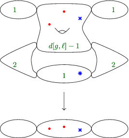
Each of the two rational components mapping with degree 2 must carry two of the ramification points. The total number of loci of the form (14) is therefore given by
 \begin{equation} \frac{1}{2} \binom{b[d,\ell]}{2,2,b[d,\ell]-4} = \frac{1}{8} \frac{b[d,\ell]!}{(b[d,\ell]-4)!} \,,\end{equation}
with the factor
 $1/2$
corresponding to the fact that the two pairs of branch points going to the outer components can be exchanged without changing the locus.
$1/2$
corresponding to the fact that the two pairs of branch points going to the outer components can be exchanged without changing the locus.
For
 $r>1$
, the locus is parametrised by the space
$r>1$
, the locus is parametrised by the space
 \begin{equation} \overline{\mathcal{H}}_{(\Gamma, \Gamma')} = \overline{\mathcal{H}}_{g-1,d[g,\ell]-1,n[g,\ell]-1+2,r-1} \times\underbrace{ \overline{\mathcal{H}}_{0,2,2,2} \times \overline{\mathcal{H}}_{0,2,2,2}}_{=\{\textrm{pt}\}}\,.\end{equation}
The unique point of
 $\overline{\mathcal{H}}_{0,2,2,2}$
is given by the map
$\overline{\mathcal{H}}_{0,2,2,2}$
is given by the map
 \begin{equation*}(\mathbb{P}^1, 1, -1) \xrightarrow{z \mapsto z^2} \mathbb{P}^1\, ,\end{equation*}
and the cover has no remaining automorphisms.
On the other hand, for
 $r=1$
, the position of marking
$r=1$
, the position of marking
 $p_{n[g,\ell]}$
is no longer determined by the map and markings on the genus
$p_{n[g,\ell]}$
is no longer determined by the map and markings on the genus
 $g-1$
component. If
$g-1$
component. If
 $r=1$
, let
$r=1$
, let
 \begin{equation*}\widehat{\epsilon}_0 \;:\; \overline{\mathcal{H}}_{g-1,d[g,\ell]-1,n[g,\ell]-1+2,r-1} \to\; \overline{\mathcal{M}}_{0,4g+2\ell-4+n[g,\ell]-1}\end{equation*}
be the map remembering both the
 $4g+2\ell-4$
branch points and the images of the
$4g+2\ell-4$
branch points and the images of the
 $n[g,\ell]-1$
markings on the target of the cover. Then the locus fits into a diagram
$n[g,\ell]-1$
markings on the target of the cover. Then the locus fits into a diagram

where the right vertical arrow is the map forgetting the last marking.
Since, independent of r, the map (14) is unramified at all the nodes, we see from [Reference Lian18, proposition 3·3] that the locus
 $\overline{\mathcal{H}}_{(\Gamma, \Gamma')}$
appears with multiplicity 1 in the upper fibre diagram (13). On the other hand, there are 8 different
$\overline{\mathcal{H}}_{(\Gamma, \Gamma')}$
appears with multiplicity 1 in the upper fibre diagram (13). On the other hand, there are 8 different
 $\widehat{\Gamma}_0$
-structures on the graph
$\widehat{\Gamma}_0$
-structures on the graph
 $\Gamma$
of the domain curve in (14) that satisfy the assumptions of [Reference Lian18, proposition 3·2]. Indeed, the image of the first edge of
$\Gamma$
of the domain curve in (14) that satisfy the assumptions of [Reference Lian18, proposition 3·2]. Indeed, the image of the first edge of
 $\widehat{\Gamma}_0$
can be chosen freely among the 4 nonseparating edges of
$\widehat{\Gamma}_0$
can be chosen freely among the 4 nonseparating edges of
 $\Gamma$
, and then the second edge must go to one of the 2 edges on the other side. So overall, in the disjoint union in the top left of the diagram (13), there are
$\Gamma$
, and then the second edge must go to one of the 2 edges on the other side. So overall, in the disjoint union in the top left of the diagram (13), there are
 \begin{equation*}\frac{b[d,\ell]!}{(b[d,\ell]-4)!}\end{equation*}
many components that can contribute.
By the strategy explained above, we see that the contribution to the degree of
 $\tau_{g,\ell,r}^* [(C,D)]$
coming from each of the components is given by the degree of the map
$\tau_{g,\ell,r}^* [(C,D)]$
coming from each of the components is given by the degree of the map
 \begin{equation} \overline{\mathcal{H}}_{(\Gamma, \Gamma')} \to \underbrace{\overline{\mathcal{M}}_{g-1,n[g,\ell]+1}}_{=\overline{\mathcal{M}}_{\Gamma_0}} \times \overline{\mathcal{M}}_{0,n[g,\ell]-r+1}.\end{equation}
-
(i) For
$r>1$
, the locus
$\overline{\mathcal{H}}_{(\Gamma, \Gamma')}$
is given by (16) and the above map fits as the top horizontal arrow into a commutative diagram mapping birationally onto the corresponding fibre product. So the degree of the top map is the same as the degree of the bottom map. Usingthe bottom map is precisely
\begin{equation*}d[g,\ell]-1 = d[g-1,\ell]\, , \ \ \ n[g,\ell]-1 = n[g-1,\ell]\, ,\end{equation*}
$\tau_{g-1,\ell,r-1}$
.
-
(ii) For
$r=1$
, we must distinguish two more cases: -
(a) For
$n[g,\ell] \geq 4$
, the map (18) appears as the top horizontal arrow in the commutative diagram mapping birationally to the associated fibre product, and so the degree of (18) is given by the degree of the bottom map
$\tau_{g-1,\ell,1}$
.
-
(b) For
$n[g,\ell]=3$
, the map (18) factors through the left vertical map in (17). Since the vertical map drops dimension by 1, we know that the morphism (18) can no longer be dominant and thus yields a zero contribution. The vanishing here is compatible with our original definition, since
$\mathsf{Tev}_{g-1,\ell,1}$
is defined to be zero since
$n[g-1,\ell]=2$
.


Overall, we see that the total part of the degree arising from Contribution 1 is given by
 \begin{equation*}\frac{b[d,\ell]!}{(b[d,\ell]-4)!} \deg \tau_{g-1,\ell,\max(1,r-1)} = b[d,\ell]! \cdot \mathsf{Tev}_{g-1,\ell,\max(1,r-1)}\,.\end{equation*}
Contribution 2. The second type of locus that can contribute parametrises covers of the form illustrated in diagram (19).

The rational component mapping with degree 2 must carry two of the ramification points. The total number of loci of the form (19) is given by
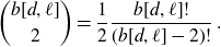 \begin{equation} \binom{b[d,\ell]}{2} = \frac{1}{2} \frac{b[d,\ell]!}{(b[d,\ell]-2)!} \,.\end{equation}
The locus
 $\overline{\mathcal{H}}_{(\Gamma, \Gamma')}$
is parametrised by the space
$\overline{\mathcal{H}}_{(\Gamma, \Gamma')}$
is parametrised by the space
 \begin{equation} \overline{\mathcal{H}}_{g-1,d[g,\ell],n[g,\ell]+1,r+1} \times \overline{\mathcal{H}}_{0,2,3,2}\,.\end{equation}
The
 $r+1$
index in (21) is explained by the following basic important observation: all
$r+1$
index in (21) is explained by the following basic important observation: all
 $r+1$
nodes of the genus
$r+1$
nodes of the genus
 $g-1$
domain component connecting to rational curves containing blue markings map to the same point (which is the node of the range curve).
$g-1$
domain component connecting to rational curves containing blue markings map to the same point (which is the node of the range curve).
The space
 $\overline{\mathcal{H}}_{0,2,3,2}$
, parametrises double covers
$\overline{\mathcal{H}}_{0,2,3,2}$
, parametrises double covers
 \begin{equation} f \;:\; (\mathbb{P}^1, p, z, z', q_1, q_2) \to \mathbb{P}^1\end{equation}
such that
 $f(z)=f(z')$
and such that
$f(z)=f(z')$
and such that
 $q_1, q_2$
are ramification points of the cover. The natural map
$q_1, q_2$
are ramification points of the cover. The natural map
 \begin{equation*}\delta \;:\; \overline{\mathcal{H}}_{0,2,3,2} \to \overline{\mathcal{M}}_{0,4}\end{equation*}
sending the point (22) to
 \begin{equation*}(\mathbb{P}^1,\; f(p),\; f(z),\; f(q_1),\; f(q_2)) \in \overline{\mathcal{M}}_{0,4}\end{equation*}
has degree 2, corresponding to the two choices z, z ′ of preimage of f(z).
By the same argument as before, the loci (19) appear with multiplicity 1 in the upper fibre diagram (13). On the other hand, there are 2
 $\widehat{\Gamma}_0$
-structures on the graph
$\widehat{\Gamma}_0$
-structures on the graph
 $\Gamma$
of the domain curve in (19), corresponding to the two choices of sending the edges of
$\Gamma$
of the domain curve in (19), corresponding to the two choices of sending the edges of
 $\widehat{\Gamma}_0$
to the two nonseparating edges e, e
′ of
$\widehat{\Gamma}_0$
to the two nonseparating edges e, e
′ of
 $\Gamma$
. However, these two
$\Gamma$
. However, these two
 $\widehat{\Gamma}_0$
-structures are isomorphic (since the cover
$\widehat{\Gamma}_0$
-structures are isomorphic (since the cover
 $\Gamma \to \Gamma'$
has an automorphism exchanging the two edges e, e
′). So overall, in the disjoint union in the top left of the diagram (13) there are
$\Gamma \to \Gamma'$
has an automorphism exchanging the two edges e, e
′). So overall, in the disjoint union in the top left of the diagram (13) there are
 \begin{equation*}\frac{1}{2} \cdot \frac{b[d,\ell]!}{(b[d,\ell]-2)!}\end{equation*}
many components that can contribute.
However, a new phenomenon (not seen in Contribution 1) appears here: a dimension count shows that the loci (21) only have codimension 1 in their ambient space, whereas the gluing map
 $\xi_{\Gamma_0}$
had codimension 2. The excess class is given by
$\xi_{\Gamma_0}$
had codimension 2. The excess class is given by
 \begin{equation*}- \psi_{w} \otimes 1 - 1 \otimes \psi_{z},\end{equation*}
where w, z are the preimages of one of the nonseparating nodes in (19), see [Reference Schmitt and van Zelm25, section 4·2] and [Reference Lian18, proposition 3·3]. The class
 $\psi_{z}$
on
$\psi_{z}$
on
 $\overline{\mathcal{H}}_{0,2,3,2}$
is the pullback of
$\overline{\mathcal{H}}_{0,2,3,2}$
is the pullback of
 $\psi_2$
on
$\psi_2$
on
 $\overline{\mathcal{M}}_{0,4}$
under the map
$\overline{\mathcal{M}}_{0,4}$
under the map
 $\delta$
above. We calculate
$\delta$
above. We calculate
 \begin{equation*}\int_{\overline{\mathcal{H}}_{0,2,3,2}} \psi_{z} = \deg(\delta) \cdot \int_{\overline{\mathcal{M}}_{0,4}} \psi_2 = 2 \cdot 1 = 2\,.\end{equation*}
The contribution to the degree of
 $\tau_{g,\ell,r}^* [(C,D)]$
coming from each locus above is given by the degree of the excess class capped with the preimage of a point under the map
$\tau_{g,\ell,r}^* [(C,D)]$
coming from each locus above is given by the degree of the excess class capped with the preimage of a point under the map
 \begin{equation*}\overline{\mathcal{H}}_{g-1,d[g,\ell],n[g,\ell]+1,r+1} \times \overline{\mathcal{H}}_{0,2,3,2} \rightarrow \overline{\mathcal{M}}_{g-1,n[g,\ell]+1} \times \overline{\mathcal{M}}_{0,n[g,\ell]-r+1}\, .\end{equation*}
Since the above map does not depend on the factor
 $\overline{\mathcal{H}}_{0,2,3,2}$
in the domain, the only nonzero contribution can come from the term
$\overline{\mathcal{H}}_{0,2,3,2}$
in the domain, the only nonzero contribution can come from the term
 $-1 \otimes \psi_{z}$
. After eliminating the factor
$-1 \otimes \psi_{z}$
. After eliminating the factor
 $\overline{\mathcal{H}}_{0,2,3,2}$
by integrating
$\overline{\mathcal{H}}_{0,2,3,2}$
by integrating
 $-1 \otimes \psi_{z}$
(and obtaining a factor
$-1 \otimes \psi_{z}$
(and obtaining a factor
 $-2$
from the degree of
$-2$
from the degree of
 $-\psi_z$
), we are left with the degree of
$-\psi_z$
), we are left with the degree of
 $\tau_{g-1,\ell+1,r+1}$
.
$\tau_{g-1,\ell+1,r+1}$
.
The total part of the degree arising from Contribution 2 is given by
 \begin{equation*} \frac{1}{2} \cdot \frac{b[d,\ell]!}{(b[d,\ell]-2)!} \cdot (-2) \cdot \deg \tau_{g-1,\ell+1,r+1} = - b[d,\ell]! \cdot \mathsf{Tev}_{g-1,\ell+1,r+1}\,.\end{equation*}
Contribution 3. The third type of locus that can contribute parametrises covers of the form illustrated in diagram (23).
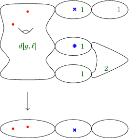
The rational component mapping with degree 2 must carry two of the ramification points. The total number of loci of the form (19) is given by
 \begin{equation} \binom{b[d,\ell]}{2} = \frac{1}{2} \frac{b[d,\ell]!}{(b[d,\ell]-2)!} \,.\end{equation}
The locus
 $\overline{\mathcal{H}}_{(\Gamma, \Gamma')}$
is parametrised by the space
$\overline{\mathcal{H}}_{(\Gamma, \Gamma')}$
is parametrised by the space
 \begin{equation} \overline{\mathcal{H}}_{g-1,d[g,\ell],n[g,\ell]+1,r+1} \times \underbrace{\overline{\mathcal{H}}_{0,2,2,2}}_{=\{\textrm{pt}\}}\,.\end{equation}
Again the multiplicity is 1, but there are 4 non-isomorphic
 $\widehat{\Gamma}_0$
-structures on the graph
$\widehat{\Gamma}_0$
-structures on the graph
 $\Gamma$
: one of the two edges of
$\Gamma$
: one of the two edges of
 $\widehat{\Gamma}_0$
must go to the edge of
$\widehat{\Gamma}_0$
must go to the edge of
 $\Gamma$
connecting the genus
$\Gamma$
connecting the genus
 $g-1$
vertex to the vertex containing the last marking. The other can go to either one of the two edges incident to the vertex with the degree 2 map. So overall, in the disjoint union in the top left of the diagram (13) there are
$g-1$
vertex to the vertex containing the last marking. The other can go to either one of the two edges incident to the vertex with the degree 2 map. So overall, in the disjoint union in the top left of the diagram (13) there are
 \begin{equation*} 2 \frac{b[d,\ell]!}{(b[d,\ell]-2)!}\end{equation*}
components that can contribute.
By the strategy explained above, the contribution to the degree of
 $\tau_{g,\ell,r}^* [(C,D)]$
coming from each locus above is given by the degree of the map
$\tau_{g,\ell,r}^* [(C,D)]$
coming from each locus above is given by the degree of the map
 \begin{equation*}\overline{\mathcal{H}}_{g-1,d[g,\ell],n[g,\ell]+1,r+1} \to \overline{\mathcal{M}}_{g-1,n[g,\ell]+1} \times \overline{\mathcal{M}}_{0,n[g,\ell]-r+1}.\end{equation*}
The total part of the degree arising from Contribution 3 is given by
 \begin{equation*} \frac{1}{2} \cdot 2 \cdot \frac{b[d,\ell]!}{(b[d,\ell]-2)!} \cdot 2 \cdot \deg \tau_{g-1,\ell+1,r+1} = 2 b[d,\ell]! \cdot \mathsf{Tev}_{g-1,\ell+1,r+1}\,.\end{equation*}
Exclusion of other components.
To conclude, we must prove that Contributions 1, 2 and 3 are the only loci in the diagram (13) that can contribute.
Let
 $\overline{\mathcal{H}}_{(\Gamma, \Gamma')}$
be a locus in (13) dominating the moduli space
$\overline{\mathcal{H}}_{(\Gamma, \Gamma')}$
be a locus in (13) dominating the moduli space
 \begin{equation*}\overline{\mathcal{M}}_{g-1,n[g,\ell]+1} \times \overline{\mathcal{M}}_{0,n[g,\ell]-r+1}\,.\end{equation*}
There must then be a vertex
 $v_{g-1} \in V(\Gamma)$
such that the corresponding factor of
$v_{g-1} \in V(\Gamma)$
such that the corresponding factor of
 $\overline{\mathcal{H}}_{(\Gamma, \Gamma')}$
parametrises covers from a genus
$\overline{\mathcal{H}}_{(\Gamma, \Gamma')}$
parametrises covers from a genus
 $g-1$
curve. Since the
$g-1$
curve. Since the
 $n[g,\ell]-1$
first markings will go to the vertex
$n[g,\ell]-1$
first markings will go to the vertex
 $v_{g-1}$
after forgetting the ramification points and stabilising, their images in
$v_{g-1}$
after forgetting the ramification points and stabilising, their images in
 $\Gamma'$
will similarly stabilise to a unique vertex
$\Gamma'$
will similarly stabilise to a unique vertex
 $v_0$
. Therefore, in the cover
$v_0$
. Therefore, in the cover
 $\Gamma \to \Gamma'$
, the vertex
$\Gamma \to \Gamma'$
, the vertex
 $v_{g-1}$
maps to
$v_{g-1}$
maps to
 $v_0$
. Next, we observe that the map
$v_0$
. Next, we observe that the map
 \begin{equation} \overline{\mathcal{H}}_{(\Gamma, \Gamma')} \to \overline{\mathcal{M}}_{g-1,n[g,\ell]+1} \times \overline{\mathcal{M}}_{0,n[g,\ell]-r+1}\end{equation}
only depends upon the factors of
 $\overline{\mathcal{H}}_{(\Gamma, \Gamma')}$
lying over the vertex
$\overline{\mathcal{H}}_{(\Gamma, \Gamma')}$
lying over the vertex
 $v_0$
. Indeed, the map to
$v_0$
. Indeed, the map to
 $\overline{\mathcal{M}}_{g-1,n[g,\ell]+1}$
only depends on the factor for
$\overline{\mathcal{M}}_{g-1,n[g,\ell]+1}$
only depends on the factor for
 $v_{g-1}$
. On the other hand, since the stabilisation of
$v_{g-1}$
. On the other hand, since the stabilisation of
 $\Gamma'$
, after forgetting the branch points, consists of the single vertex
$\Gamma'$
, after forgetting the branch points, consists of the single vertex
 $v_0$
, the factors of
$v_0$
, the factors of
 $\overline{\mathcal{H}}_{(\Gamma, \Gamma')}$
over
$\overline{\mathcal{H}}_{(\Gamma, \Gamma')}$
over
 $v_0$
determine the component of the map (26) to
$v_0$
determine the component of the map (26) to
 $\overline{\mathcal{M}}_{0,n[g,\ell]-r+1}$
.
$\overline{\mathcal{M}}_{0,n[g,\ell]-r+1}$
.
Since the factors over
 $v_0$
form a finite cover of the moduli space
$v_0$
form a finite cover of the moduli space
 $\overline{\mathcal{M}}_{0,n(v_0)}$
associated to
$\overline{\mathcal{M}}_{0,n(v_0)}$
associated to
 $v_0$
, the valence
$v_0$
, the valence
 $n(v_0)$
must satisfy
$n(v_0)$
must satisfy
 \begin{equation*}n(v_0) - 3 \geq \dim\ \overline{\mathcal{M}}_{g-1,n[g,\ell]+1} \times \overline{\mathcal{M}}_{0,n[g,\ell]-r+1} = b[g,\ell] + n[g,\ell] -r -4\end{equation*}
in order for the map (26) to be dominant.
A short computation shows that the valence condition is only possible in one of the following cases:
-
(i)
$\Gamma'$
has two other vertices
$w_1, w_2$
, both of valence 3; -
(ii)
$\Gamma'$
has one other vertex w, of valence 4; -
(iii)
$\Gamma'$
has one other vertex w, of valence 3.


We further observe that for a simple branch point at the vertex
 $v_0$
whose ramification point is not on the component associated to
$v_0$
whose ramification point is not on the component associated to
 $v_{g-1}$
, the position of the branch point does not affect the image under the map (26). Therefore, in cases (i) and (ii) all the simple ramification points over
$v_{g-1}$
, the position of the branch point does not affect the image under the map (26). Therefore, in cases (i) and (ii) all the simple ramification points over
 $v_0$
are located at the vertex
$v_0$
are located at the vertex
 $v_{g-1}$
, whereas in case (iii) at most one of them can be on a separate component.
$v_{g-1}$
, whereas in case (iii) at most one of them can be on a separate component.
Finally, we observe that for every leaf of the graph
 $\Gamma'$
which is not equal to
$\Gamma'$
which is not equal to
 $v_0$
(so one of the vertices
$v_0$
(so one of the vertices
 $w,w_1,w_2$
above), the leaf must contain at least two of the simple branch points. Indeed, by the condition that there is a
$w,w_1,w_2$
above), the leaf must contain at least two of the simple branch points. Indeed, by the condition that there is a
 $\widehat{\Gamma}_0$
structure on
$\widehat{\Gamma}_0$
structure on
 $\Gamma \to \Gamma'$
, there must be a circular path from
$\Gamma \to \Gamma'$
, there must be a circular path from
 $v_{g-1}$
to itself in
$v_{g-1}$
to itself in
 $\Gamma$
whose edges surject to the edges of
$\Gamma$
whose edges surject to the edges of
 $\Gamma'$
. Thus over a leaf there must be a vertex with at least two edges adjacent, which needs at least two ramification points on that vertex.
$\Gamma'$
. Thus over a leaf there must be a vertex with at least two edges adjacent, which needs at least two ramification points on that vertex.
Case (i). There are two possibilities
 $\Gamma'_{\!\!1}$
and
$\Gamma'_{\!\!1}$
and
 $\Gamma'_{\!\!2}$
for the graph
$\Gamma'_{\!\!2}$
for the graph
 $\Gamma'$
.
$\Gamma'$
.

By the general comments above, the two markings at
 $w_2$
must be branch points, and we see that there are at least
$w_2$
must be branch points, and we see that there are at least
 $b[g,\ell]-3$
simple ramification points at
$b[g,\ell]-3$
simple ramification points at
 $v_{g-1}$
. The configuration is only possible if the degree at the vertex
$v_{g-1}$
. The configuration is only possible if the degree at the vertex
 $v_{g-1}$
remains at
$v_{g-1}$
remains at
 $d[g,\ell]$
, otherwise the number of ramification points would drop by at least 4. The marking at
$d[g,\ell]$
, otherwise the number of ramification points would drop by at least 4. The marking at
 $w_1$
is then forced to be the image of the marking
$w_1$
is then forced to be the image of the marking
 $p_{n[g,\ell]}$
, since otherwise this marking would be contained in the genus
$p_{n[g,\ell]}$
, since otherwise this marking would be contained in the genus
 $g-1$
component of the curve, contradicting the shape (12) we have fixed before. We conclude that only the pair
$g-1$
component of the curve, contradicting the shape (12) we have fixed before. We conclude that only the pair
 $(\Gamma, \Gamma'_{\!\!1})$
of Contribution 3 has the specified shape.
$(\Gamma, \Gamma'_{\!\!1})$
of Contribution 3 has the specified shape.

The markings at
 $w_1, w_2$
belonging to branch points, so we have precisely
$w_1, w_2$
belonging to branch points, so we have precisely
 $b[g,\ell]-4$
branch points at
$b[g,\ell]-4$
branch points at
 $v_0$
. Then the component
$v_0$
. Then the component
 $v_{g-1}$
must have degree
$v_{g-1}$
must have degree
 $d[g,\ell]-1$
, so that there is an additional vertex of genus 0 over
$d[g,\ell]-1$
, so that there is an additional vertex of genus 0 over
 $v_0$
mapping with degree 1. We are then forced to be in the case of Contribution 1.
$v_0$
mapping with degree 1. We are then forced to be in the case of Contribution 1.
Case (ii). The shape of the graph
 $\Gamma'$
is as follows:
$\Gamma'$
is as follows:

Since there are at least
 $b[g,\ell]-3$
simple branch points at
$b[g,\ell]-3$
simple branch points at
 $v_0$
, the component
$v_0$
, the component
 $v_{g-1}$
must map with full degree
$v_{g-1}$
must map with full degree
 $d[g,\ell]$
. Therefore, one of the three markings at w is forced to be the image of marking
$d[g,\ell]$
. Therefore, one of the three markings at w is forced to be the image of marking
 $p_{n[g,\ell]}$
. Moreover, the point
$p_{n[g,\ell]}$
. Moreover, the point
 $p_{n[g,\ell]}$
must lie on the unique loop in
$p_{n[g,\ell]}$
must lie on the unique loop in
 $\Gamma$
which goes through the vertex over w containing the two ramification points. We are in the case of Contribution 2.
$\Gamma$
which goes through the vertex over w containing the two ramification points. We are in the case of Contribution 2.
Case (iii). The graph
 $\Gamma'$
has the following shape:
$\Gamma'$
has the following shape:

The markings at w are branch points, so the remaining
 $b[g,\ell]-2$
branch points are at
$b[g,\ell]-2$
branch points are at
 $v_0$
. As we have seen before, in case (iii), at most one of the associated ramification points can be on a component not equal to
$v_0$
. As we have seen before, in case (iii), at most one of the associated ramification points can be on a component not equal to
 $v_{g-1}$
, which still forces
$v_{g-1}$
, which still forces
 $b[g,\ell]-3$
ramification points on
$b[g,\ell]-3$
ramification points on
 $v_{g-1}$
. The component
$v_{g-1}$
. The component
 $v_{g-1}$
must map with full degree
$v_{g-1}$
must map with full degree
 $d[g,\ell]$
. Hence we arrive at a contradiction, since the marking
$d[g,\ell]$
. Hence we arrive at a contradiction, since the marking
 $p_{n[g,\ell]}$
lies over
$p_{n[g,\ell]}$
lies over
 $v_0$
and thus in
$v_0$
and thus in
 $v_{g-1}$
. The curve can not have the shape (12).
$v_{g-1}$
. The curve can not have the shape (12).
Contributions 1,2 and 3 are therefore the only nonvanishing terms in the intersection. After summing the three contributions to the degree of
 $\tau_{g,\ell,r}$
and dividing by
$\tau_{g,\ell,r}$
and dividing by
 $b[d,\ell]!$
, we obtain the recursion stated in the Proposition.
$b[d,\ell]!$
, we obtain the recursion stated in the Proposition.
4. Proof of Theorems 1-3 for
$\ell\geq 0$

4·1. The genus 0 case
The recursion of Proposition 7 reduces the calculation of the degree of
 $\tau_{g,\ell,r}$
to the genus
$\tau_{g,\ell,r}$
to the genus
 $g=0$
case. Indeed, for
$g=0$
case. Indeed, for
 $n[g,\ell]-r+1 \geq 3$
, we can apply the recursion and lower the genus and, for
$n[g,\ell]-r+1 \geq 3$
, we can apply the recursion and lower the genus and, for
 $n[g,\ell]-r+1 < 3$
,
$n[g,\ell]-r+1 < 3$
,
 $\mathsf{Tev}_{g,\ell,r}$
is defined to be 0. In genus 0, since
$\mathsf{Tev}_{g,\ell,r}$
is defined to be 0. In genus 0, since
 \begin{equation*}1 \leq r \leq d[0,\ell] = \ell+1\, \end{equation*}
by (3), we must have
 $\ell\geq 0$
. The Tevelev degrees in genus 0 for
$\ell\geq 0$
. The Tevelev degrees in genus 0 for
 $\ell\geq 0$
are determined by the following result.
$\ell\geq 0$
are determined by the following result.
Proposition 8. For
 $\ell \geq 0$
and
$\ell \geq 0$
and
 $1\leq r \leq \ell +1$
we have
$1\leq r \leq \ell +1$
we have
 \begin{equation*} \mathsf{Tev}_{0,\ell,r}=1.\end{equation*}
Proof. Let
 $(\mathbb{P}^1, p_1,\ldots,p_n)$
be a genus 0 curve with n distinct markings, for
$(\mathbb{P}^1, p_1,\ldots,p_n)$
be a genus 0 curve with n distinct markings, for
 \begin{equation*}n=n[0,\ell]=3+2\ell \geq 3\, .\end{equation*}
Let
 $\mathcal{M}_{d,r}$
be the moduli space of maps
$\mathcal{M}_{d,r}$
be the moduli space of maps
 \begin{equation*}\pi \;:\; (\mathbb{P}^1,p_1,\ldots,p_n) \to \mathbb{P}^1\end{equation*}
of degree
 $d[0,\ell]=1+\ell$
satisfying
$d[0,\ell]=1+\ell$
satisfying
 \begin{equation*}\pi(p_{n-r+1}) = \cdots = \pi(p_n)= [1,0]\in \mathbb{P}^1\, .\end{equation*}
The moduli space
 $\mathcal{M}_{d,r}$
is the nonsingular
$\mathcal{M}_{d,r}$
is the nonsingular
 $n-r$
dimensional quasi-projective subvariety
$n-r$
dimensional quasi-projective subvariety
 \begin{equation*}\mathcal{M}_{d,r} \subset\mathbb{P}(H^0(\mathbb{P}^1,\mathcal{O}_{\mathbb{P}^1}(d)) \oplus H^0(\mathbb{P}^1,\mathcal{O}_{\mathbb{P}^1}(d)))\ \end{equation*}
defined by pairs of sections
 $(s_0,s_1)$
of
$(s_0,s_1)$
of
 $H^0(\mathbb{P}^1,\mathcal{O}_{\mathbb{P}^1}(d))$
satisfying:
$H^0(\mathbb{P}^1,\mathcal{O}_{\mathbb{P}^1}(d))$
satisfying:
-
(i)
$s_0$
and
$s_1$
have no common zeros; -
(ii)
$s_1$
vanishes at the r points
$p_{n-r+1}$
,…,
$p_n$
.


Conditions (ii) are linear, so
 $\mathcal{M}_{d,r}\subset \mathbb{P}^{2d+1-r}= \mathbb{P}^{n-r}$
.
$\mathcal{M}_{d,r}\subset \mathbb{P}^{2d+1-r}= \mathbb{P}^{n-r}$
.
The tangent space of
 $\mathcal{M}_{d,r}$
at
$\mathcal{M}_{d,r}$
at
 $[\pi]\in \mathcal{M}_{d,r}$
is
$[\pi]\in \mathcal{M}_{d,r}$
is
 \begin{equation*} \mathsf{Tan}_\pi =H^0(\mathbb{P}^1, \pi^*(\mathsf{Tan}_{\mathbb{P}^1})(-p_{n-r+1}-\cdots-p_n))\, .\end{equation*}
The degree of the line bundle
 $\pi^*(\mathsf{Tan}_{\mathbb{P}^1})(-p_{n-r+1}-\ldots-p_n)$
is
$\pi^*(\mathsf{Tan}_{\mathbb{P}^1})(-p_{n-r+1}-\ldots-p_n)$
is
 \begin{equation*}2(1+\ell) - r =n-r-1\, .\end{equation*}
Since the points
 $p_1,\ldots,p_{n-r}$
impose independent conditions on sections of
$p_1,\ldots,p_{n-r}$
impose independent conditions on sections of
 $\pi^*(\mathsf{Tan}_{\mathbb{P}^1})(-p_{n-r+1}-\cdots-p_n)$
, the differential of the evaluation map
$\pi^*(\mathsf{Tan}_{\mathbb{P}^1})(-p_{n-r+1}-\cdots-p_n)$
, the differential of the evaluation map
 \begin{equation*}\text{ev}\;:\;\mathcal{M}_{d,r} \to (\mathbb{P}^1)^{n-r}\, , \ \ \ \ [\pi]\longmapsto (\pi(p_1),\cdots,\pi(p_{n-r}))\end{equation*}
is surjective.
Let
 $x_1\,\ldots,x_{n-r}\in \mathbb{P}^1$
be general points. For
$x_1\,\ldots,x_{n-r}\in \mathbb{P}^1$
be general points. For
 $1\leq i \leq n-r$
, let
$1\leq i \leq n-r$
, let
 \begin{equation*}\mathsf{H}_i\subset \mathcal{M}_{d,r}\end{equation*}
be the locus of maps
 $\pi$
satisfying
$\pi$
satisfying
 \begin{equation*}\pi(p_i)=x_i\, .\end{equation*}
The closure
 $\overline{\mathsf{H}}_i\subset\mathbb{P}^{2d+n-r}$
is a linear space of codimension 1. Since
$\overline{\mathsf{H}}_i\subset\mathbb{P}^{2d+n-r}$
is a linear space of codimension 1. Since
 \begin{equation}\mathsf{ev}^{-1}(x_1,\ldots,x_{n-r})\subset \mathcal{M}_{d,r}\end{equation}
is both transverse and linear,
 $\mathsf{ev}^{-1}(x_1,\ldots,x_{n-r})$
is either empty or a reduced point. Since the image of ev is dense,
$\mathsf{ev}^{-1}(x_1,\ldots,x_{n-r})$
is either empty or a reduced point. Since the image of ev is dense,
 $\mathsf{ev}^{-1}(x_1,\ldots,x_{n-r})$
must be a reduced point.Footnote
14
$\mathsf{ev}^{-1}(x_1,\ldots,x_{n-r})$
must be a reduced point.Footnote
14
Finally, a dimension count shows the single reduced point (27) corresponds to a map with only simple ramification points. Therefore,
 $\mathsf{Tev}_{0,\ell,r}=1$
.
$\mathsf{Tev}_{0,\ell,r}=1$
.
4·2. Induction argument
We are ready to completely calculate the Tevelev degrees in case
 $\ell \geq 0$
. Because of the form of the recursion (11), we consider all the cases with
$\ell \geq 0$
. Because of the form of the recursion (11), we consider all the cases with
 $\ell \geq 0$
at once instead of proving Theorems 1, 2 and 3 separately.
$\ell \geq 0$
at once instead of proving Theorems 1, 2 and 3 separately.
Theorem. For
 $g \geq 0$
,
$g \geq 0$
,
 $ \ell \geq 0$
and
$ \ell \geq 0$
and
 $1 \leq r \leq \ell +1 +g$
, we have
$1 \leq r \leq \ell +1 +g$
, we have
 \begin{equation*}\mathsf{Tev}_{g,l,r}=\begin{cases}2^g- \sum_{j=0}^{r-2} \left(\begin{matrix} {g} \\ {j} \end{matrix}\right) &\text{for } \ell =0,\\ \mathsf{Tev}_{g,0,\max(r-\ell,1)} & \text{for } \ell \leq r,\\ 2^g & \text{for } \ell\geq r.\end{cases}\end{equation*}
Proof. We proceed by induction on g. The
 $g=0$
case is covered by Proposition 8. Suppose
$g=0$
case is covered by Proposition 8. Suppose
 $g > 0$
.
$g > 0$
.
Step 1. We consider the case
 $ \ell \geq r \geq 1$
. If we start with
$ \ell \geq r \geq 1$
. If we start with
 $ \ell \geq r$
, the same inequality persists for the recursion, and we have
$ \ell \geq r$
, the same inequality persists for the recursion, and we have
 \begin{equation*} \mathsf{Tev}_{g,\ell,r}= \mathsf{Tev}_{g-1,\ell,\max(1,r-1)}+ \mathsf{Tev}_{g-1,\ell+1,r+1}= 2^{g-1}+ 2^{g-1}=2^g\,. \end{equation*}
Step 2. We consider case
 $0\leq \ell \leq r$
. We have already checked the case
$0\leq \ell \leq r$
. We have already checked the case
 $\ell =r$
. Suppose
$\ell =r$
. Suppose
 $ \ell < r$
. If we start with
$ \ell < r$
. If we start with
 $ \ell < r$
, then the non-strict inequality
$ \ell < r$
, then the non-strict inequality
 $ \ell \leq r$
persists in the first step of the recursion. We have
$ \ell \leq r$
persists in the first step of the recursion. We have
 \begin{align*}\mathsf{Tev}_{g,\ell,r}& =\mathsf{Tev}_{g-1,\ell ,\max(r - 1,1)} + \mathsf{Tev}_{g-1,\ell+1,r+1}\\& = 2^{g-1}- \sum_{j=0}^{ \max(r-3-\ell,-1 - \ell) } \left(\begin{matrix} { g-1} \\ {j} \end{matrix}\right) + 2^{g-1} - \sum_{j=0}^{ r-2-\ell } \left(\begin{matrix}{ g-1} \\ {j} \end{matrix}\right) \\& = 2^g - \sum_{j=0}^{ r-2-\ell } \Bigg[ \left(\begin{matrix} { g-1} \\ {j-1} \end{matrix}\right) + \left(\begin{matrix} {g-1} \\ {j} \end{matrix} \right) \Bigg]\\ &= 2^g - \sum_{j=0}^{ r-2-\ell } \left( \begin{matrix} { g} \\ {j} \end{matrix}\right) \ , \end{align*}
where in the first equality we are using the inductive step applied to g.
The proof is complete.
4·3. Lines in projective space
By the formulas of Theorems 2 and 3, we have
 \begin{equation}\mathsf{Tev}_{g,\ell,g+1+\ell}=1\, .\end{equation}
The Tevelev degree is defined via the map
 \begin{equation*}\tau_{g,\ell,g+1+\ell} \;:\; \overline{\mathcal{H}}_{g,g+1+\ell,g+3+2\ell,g+1+\ell} \to\overline{\mathcal{M}}_{g,g+3+2\ell}\times\overline{\mathcal{M}}_{0,3+\ell}\, .\end{equation*}
There is a simple geometric reason for the Tevelev degree to be 1 here.
Let
 $(C,p_1,\ldots,p_{g+3+2\ell})$
be a general nonsingular pointed curve. The last
$(C,p_1,\ldots,p_{g+3+2\ell})$
be a general nonsingular pointed curve. The last
 $g+1+\ell$
markings (associated to r) determine a line bundle L on C. Consider the complete linear series
$g+1+\ell$
markings (associated to r) determine a line bundle L on C. Consider the complete linear series
 $\mathbb{P}(H^0(C,L))$
of dimension
$\mathbb{P}(H^0(C,L))$
of dimension
 $1+\ell$
by Riemann–Roch.
$1+\ell$
by Riemann–Roch.
-
(i) There is a distinguished element
\begin{equation*}\zeta =[p_{3+\ell}+ \cdots +p_{g+3+2\ell}]\in \mathbb{P}(H^0(C,L))\, .\end{equation*}
-
(ii) There are
$2+\ell$
distinguished hyperplanes determined by the points
\begin{equation*}\mathsf{H}_1,\ldots, \mathsf{H}_{2+\ell} \subset \mathbb{P}(H^0(C,L))\end{equation*}
$p_1,\ldots,p_{2+\ell} \in C$
.
-
(iii) There is a projective space
$\mathbb{P}(\mathsf{Tan}_\zeta)$
of dimension
$\ell$
parametrising lines passing through
\begin{equation*}\mathsf{P}\subset \mathbb{P}(H^0(C,L))\end{equation*}
$\zeta$
.


For a general such line
 $\mathsf{P}$
, we obtain a
$\mathsf{P}$
, we obtain a
 $3+\ell$
pointed curve of genus 0,
$3+\ell$
pointed curve of genus 0,
 \begin{equation*}(\mathsf{P}, \zeta, \mathsf{P}\cap \mathsf{H}_1,\ldots, \mathsf{P}\cap\mathsf{H}_{2+\ell})\, .\end{equation*}
The associated rational map
 \begin{equation}\mathbb{P}(\mathsf{Tan}_\zeta)\dashrightarrow\mathcal{M}_{0,3+\ell}\end{equation}
is easily seen to be birational (of degree 1). The degree is
 $\mathsf{Tev}_{g,\ell,g+1+\ell}$
.
$\mathsf{Tev}_{g,\ell,g+1+\ell}$
.
The map (29) has the flavour of a Gale transformation. In the
 $\ell=1$
case, a direct connection to the Gale transformation can be made. Whether the birationality of (29) can be explained for all
$\ell=1$
case, a direct connection to the Gale transformation can be made. Whether the birationality of (29) can be explained for all
 $\ell$
in terms of the Gale transformation is a question left to the reader.
$\ell$
in terms of the Gale transformation is a question left to the reader.
5. Path counting
5·1. Notation
We consider here the case
 $\ell \leq 0$
and prove Theorem 4. Before presenting the proof, we briefly recall the notation of Section 1·4.
$\ell \leq 0$
and prove Theorem 4. Before presenting the proof, we briefly recall the notation of Section 1·4.
For
 $\ell \leq 0$
and
$\ell \leq 0$
and
 $r \geq 1 $
, we have
$r \geq 1 $
, we have
 \begin{equation*}n[g, \ell]=3+g+2 \ell\, .\end{equation*}
After imposing
 $n[g, \ell]-(r-1) \geq 3$
, we obtain the condition
$n[g, \ell]-(r-1) \geq 3$
, we obtain the condition
 \begin{equation*}g \geq r-2 \ell-1\, .\end{equation*}
Following the notation of Section 1·4,
 \begin{equation*}g[ \ell, r]= r - 2 \ell -1\, . \end{equation*}
We also have
 \begin{equation*}d[g[\ell,r],\ell]=g[\ell,r]+1+\ell =r-\ell>0\,.\end{equation*}
Define the infinite vectors
 $\mathsf{T}_{\ell, r}$
and
$\mathsf{T}_{\ell, r}$
and
 $\mathsf{E}_r$
by
$\mathsf{E}_r$
by
 \begin{equation*}\mathsf{T}_{\ell,r}[j]= \mathsf{Tev}_{g[\ell,r]+j, \ell,r}\ \ \ \text{and} \ \ \ \mathsf{E}_{r}[j] = 2^{r+j-1} - \sum_{i=0}^{r-2}\binom{r+j-1}{i}\,\end{equation*}
for
 $j \geq 0$
. We set
$j \geq 0$
. We set
 \begin{equation*}\mathsf{T}_{\ell,r}[j]= 0\ \ \ \text{and} \ \ \ \mathsf{E}_{r}[j]=0\end{equation*}
for
 $j < 0$
. For all
$j < 0$
. For all
 $j \in \mathbb{Z}$
and
$j \in \mathbb{Z}$
and
 $r \geq 1$
, we have
$r \geq 1$
, we have
 \begin{equation} \mathsf{E}_{r+1}[j+1] = \mathsf{E}_{r+1}[j] +\mathsf{E}_{r}[j+1]\, .\end{equation}
5·2. Proof of Theorem 4 for
$\ell\leq 0$

By Theorems 2 and 3 for
 $\ell \geq 0$
, we already know
$\ell \geq 0$
, we already know
 \begin{equation*}\mathsf{T}_{0,r}= \mathsf{E}_{r} =\sum_{\gamma\in \mathsf{P}(0,r)}\mathsf{E}_{\mathsf{Ind}(\gamma)} \end{equation*}
holds.
We prove the formula of Theorem 4 for the coefficient
 \begin{equation*}\mathsf{T}_{\ell,r}[j]\ \ \text{for}\ j\geq 0\end{equation*}
by induction on
 $g=g[\ell,r]+j$
. When
$g=g[\ell,r]+j$
. When
 $g[\ell,r]+j=0$
, we must have
$g[\ell,r]+j=0$
, we must have
 $(\ell,r)=(0,1)$
and
$(\ell,r)=(0,1)$
and
 $j=0$
. So the base of the induction is established.
$j=0$
. So the base of the induction is established.
Suppose now
 $g[\ell,r]+j>0$
. The proof of the induction step is split into two cases:
$g[\ell,r]+j>0$
. The proof of the induction step is split into two cases:
Case 1. Suppose
 $r=1$
and
$r=1$
and
 $ \ell \leq 0$
.
$ \ell \leq 0$
.
-
(i) If
$j=0$
, we have The second equality follows from (11) since
\begin{align*}\mathsf{T}_{\ell,1}[0]&= \mathsf{Tev}_{g[\ell,1],\ell,1}\\ &= \mathsf{Tev}_{g[\ell,1]-1,\ell+1,2} \\&= \mathsf{T}_{\ell+1,2}[0] \\&=\sum_{\gamma\in \mathsf{P}(\ell +1 ,2)}\mathsf{E}_{\mathsf{Ind}(\gamma)}[0] \\&=\sum_{\gamma\in \mathsf{P}(\ell ,1)}\mathsf{E}_{\mathsf{Ind}(\gamma)}[0]\, .\end{align*}
The last equality follows from
\begin{equation*}\mathsf{Tev}_{g[\ell,1]-1,\ell,1}=\mathsf{T}_{\ell,1}[-1]=0\, .\end{equation*}
$\mathsf{E}_{\mathsf{Ind}(\gamma)}[0]=1$
for all
$\gamma\in \mathsf{P}(\ell ,1) \cup \mathsf{P}(\ell +1 ,2)$
and the fact that
$\mathsf{P}(\ell +1 ,2)$
and
$\mathsf{P}(\ell ,1)$
are in bijection.
-
(ii) If
$j > 0$
, we have In the fifth equality, we use the natural bijection between
\begin{align*} \mathsf{T}_{\ell,1}[j]&= \mathsf{Tev}_{g[\ell,1]+j,\ell,1}\\ & =\mathsf{Tev}_{g[\ell,1]+j-1,\ell,1}+\mathsf{Tev}_{g[\ell,1]+j-1,\ell+1,2}\\&=\mathsf{T}_{\ell,1}[j-1]+\mathsf{T}_{\ell+1,2}[j] \\& =\sum_{\gamma\in \mathsf{P}(\ell,1)}\mathsf{E}_{\mathsf{Ind}(\gamma)}[j-1]+ \sum_{\gamma\in \mathsf{P}(\ell +1 ,2)}\mathsf{E}_{\mathsf{Ind}(\gamma)}[j] \\& =\sum_{\gamma\in \mathsf{P}(\ell,1)}\mathsf{E}_{\mathsf{Ind}(\gamma)}[j-1]+ \sum_{\gamma\in \mathsf{P}(\ell ,1)}\mathsf{E}_{\mathsf{Ind}(\gamma)-1}[j] \\& = \sum_{\gamma\in \mathsf{P}(\ell,1)}\mathsf{E}_{\mathsf{Ind}(\gamma)}[j]\, .\end{align*}
$\mathsf{P}(\ell +1 ,2)$
and
$\mathsf{P}(\ell ,1)$
given by completing a path that ends in
$(\ell +1 ,2)$
to a path that ends
$(\ell ,1)$
by stepping with
$\mathsf{D}$
. In the last equality, we use (30).


Case 2. Suppose
 $r > 1$
and
$r > 1$
and
 $\ell\leq 0$
.
$\ell\leq 0$
.
For all
 $j \geq 0$
, we have a similar chain of equalities:
$j \geq 0$
, we have a similar chain of equalities:
 \begin{align*}\mathsf{T}_{\ell,r}[j]&= \mathsf{Tev}_{g[\ell,r]+j,\ell,r}\\ & =\mathsf{Tev}_{g[\ell,r]+j-1,\ell,r-1}+\mathsf{Tev}_{g[\ell,r]+j-1,\ell+1,r+1} \\&=\mathsf{T}_{\ell,r-1}[j]+\mathsf{T}_{\ell+1,r+1}[j]\\& =\sum_{\gamma\in \mathsf{P}(\ell,r-1)}\mathsf{E}_{\mathsf{Ind}(\gamma)}[j]+ \sum_{\gamma\in \mathsf{P}(\ell +1 ,r+1)}\mathsf{E}_{\mathsf{Ind}(\gamma)}[j]\\& = \sum_{\gamma\in \mathsf{P}(\ell,r)}\mathsf{E}_{\mathsf{Ind}(\gamma)}[j]\, ,\end{align*}
which completes the induction step.
5·3. Refined Dyck path counting
For
 $\ell \leq 0$
and
$\ell \leq 0$
and
 $r \geq 1$
, we can write
$r \geq 1$
, we can write
 \begin{equation}\mathsf{T}_{\ell,r}= \sum_{s=1}^{r- \ell +1} c_{\ell,r}^s \mathsf{E}_s\end{equation}
by Theorem 4 and Corollary 5. By definition,
 \begin{equation*}\mathsf{E}_1[j]=2^j\, .\end{equation*}
For
 $s\geq 2$
, define the vectors
$s\geq 2$
, define the vectors
 $\mathsf{E}'_{\!\!s}$
by
$\mathsf{E}'_{\!\!s}$
by
 \begin{equation*}\mathsf{E}'_{\!\!s} [j]= \mathsf{E}_s[j] - 2^{s-1} \mathsf{E}_1[j]\, .\end{equation*}
Then,
 $\mathsf{E}'_{\!\!s}[j]$
a polynomial in j of degree
$\mathsf{E}'_{\!\!s}[j]$
a polynomial in j of degree
 $s-2$
. The vectors
$s-2$
. The vectors
 $\mathsf{E}_s$
are therefore independent, and the coefficients
$\mathsf{E}_s$
are therefore independent, and the coefficients
 $c^s_{\ell,r}$
in (31) are unique.
$c^s_{\ell,r}$
in (31) are unique.
Table 1. Values of
 $\mathsf{T}_{\ell,r}$
for
$\mathsf{T}_{\ell,r}$
for
 $\ell<0$

By Theorem 4, the coefficient
 $c^s_{\ell,r}$
is the number of paths
$c^s_{\ell,r}$
is the number of paths
 $\gamma\in \mathsf{P}(\ell,r)$
of index s and therefore defines a refined Dyck path counting problem. The solution is given by the following result.
$\gamma\in \mathsf{P}(\ell,r)$
of index s and therefore defines a refined Dyck path counting problem. The solution is given by the following result.
Proposition 9. Let
 $ \ell \leq 0$
and
$ \ell \leq 0$
and
 $ r \geq 1$
.
$ r \geq 1$
.
-
(i) If
$\ell=0$
and
$s \in \mathbb{Z}$
, thenFootnote
15
$c_{0,r}^s= \delta^{s}_{r}$
. -
(ii) If
$\ell=-1$
and
$s \in \mathbb{Z}$
, then
$c_{-1,r}^s= \delta^{s -\delta_{r,1}}_{r+1}$
. -
(iii) If
$\ell < -1$
and
$3 \leq s \leq r- \ell +1$
, then and
\begin{equation*}c_{\ell,r}^s= \frac{(s-2)(s+r-4)}{|\ell| -2+r} \left(\begin{matrix} {|2 \ell| +r -s-1} \\ {|\ell| + 2- s} \end{matrix}\right) + \left(\begin{matrix} {{|2 \ell| +r-s-1}} \\ {{|\ell| -1}} \end{matrix}\right) - \left(\begin{matrix}{{|2 \ell| +r-s-1}} \\ {{|\ell| + r-2}} \end{matrix} \right) \end{equation*}
$c^s_{\ell,r}=0$
otherwise.


Before starting the proof, we require additional notation and an auxiliary result. For
 $(u,v),(u',v') \in \mathcal{A}$
and
$(u,v),(u',v') \in \mathcal{A}$
and
 $k \in \mathbb{Z}$
, let
$k \in \mathbb{Z}$
, let
 \begin{equation*}\mathcal{D}(k\;;\; u,v,u',v')\end{equation*}
be the set of paths
 $\gamma$
in
$\gamma$
in
 $\mathcal{A}$
from (u,v) to (u
′, v
′) which take steps U and D and meet the
$\mathcal{A}$
from (u,v) to (u
′, v
′) which take steps U and D and meet the
 $r=1$
axis
$r=1$
axis
 \begin{equation*}\{ \, (\ell,1)\, | \, \ell\leq 0\, \}\subset \mathcal{A}\end{equation*}
exactly k times. Let
 $d(k\;;\; u,v,u',v')= |\mathcal{D}(k\;;\; u,v,u',v')|$
.
$d(k\;;\; u,v,u',v')= |\mathcal{D}(k\;;\; u,v,u',v')|$
.
Lemma 10. Let
 $(u,v),(u',v') \in \mathcal{A}$
. Let
$(u,v),(u',v') \in \mathcal{A}$
. Let
 $t,j,k \in \mathbb{Z}$
satisfy
$t,j,k \in \mathbb{Z}$
satisfy
 $1 \leq t< k$
,
$1 \leq t< k$
,
 $u' \leq u$
and
$u' \leq u$
and
 $j \leq -u$
. The following equalities then hold:
$j \leq -u$
. The following equalities then hold:
-
(i)
$d(k\;;\;u+j,v,u'+j,v')=d(k\;;\;u,v,u',v')$
; -
(ii)
$d(k\;;\;0,1,u',v')=d(k\;;\;0,v',u'-v'+1,1)$
; -
(iii)
$d(k\;;\;u,v,u',v')=d(k-t\;;\;u,v+t,u',v')$
; -
(iv)
$d(k\;;\;0,1,u',1)=\left(\begin{matrix} -2 u' -k \\ -u'-k+1 \end{matrix}\right)\frac{k-1}{-u'}$
.


Proof. Identity (i) is trivial. Identities (ii)-(iv) have been proven, for example, in [Reference Scott26] by B. Scott. We sketch here his proof adapted to our notation.
Identity (ii). Every Dyck path in
 $\mathcal{A}$
from (0,1) to (u
′, v
′) can be written as a sequence of
$\mathcal{A}$
from (0,1) to (u
′, v
′) can be written as a sequence of
 $-u'$
letters D and
$-u'$
letters D and
 $- u'+v'-1$
letters U. For any such sequence, changing every D with an U and every U with a D yields a Dyck path in
$- u'+v'-1$
letters U. For any such sequence, changing every D with an U and every U with a D yields a Dyck path in
 $\mathcal{A}$
from (0,v
′) and
$\mathcal{A}$
from (0,v
′) and
 $(u'-v'+1,1)$
. Moreover, the number of intersections with the
$(u'-v'+1,1)$
. Moreover, the number of intersections with the
 $r=1$
axis of the old and the new paths are the same. Therefore, we have bijection between
$r=1$
axis of the old and the new paths are the same. Therefore, we have bijection between
 $\mathcal{D}(k;\;0,1,u',v')$
and
$\mathcal{D}(k;\;0,1,u',v')$
and
 $\mathcal{D}(k;\;0,v',u'-v'+1,1)$
.
$\mathcal{D}(k;\;0,v',u'-v'+1,1)$
.
Identity (iii). Let
 $\gamma \in \mathcal{D}(k;\;u,v,u',v')$
. For
$\gamma \in \mathcal{D}(k;\;u,v,u',v')$
. For
 $1\leq i \leq t$
, let
$1\leq i \leq t$
, let
 $(\ell_i,1)$
be the first t points at which
$(\ell_i,1)$
be the first t points at which
 $\gamma$
meets the
$\gamma$
meets the
 $r=1$
axis. Here,
$r=1$
axis. Here,
 \begin{equation*}\ell_1 < \cdots < \ell_t\, .\end{equation*}
Each of the points
 $(\ell_i,1)$
is immediately followed by a step U in
$(\ell_i,1)$
is immediately followed by a step U in
 $\gamma$
. Removing these t steps U and translating
$\gamma$
. Removing these t steps U and translating
 $\gamma$
upwards t units yields a path in
$\gamma$
upwards t units yields a path in
 $\mathcal{D}(k-t;\;u,v+t,u',v')$
. The operation is a bijection.
$\mathcal{D}(k-t;\;u,v+t,u',v')$
. The operation is a bijection.
Identity (iv). Using Identity (iii), we have
 \begin{align*}d(k;\;0,1,u',1)&=d(1;\;0,k,u',1) \\&= \binom {-2 u'-k}{-u'-k+1} - \binom{-2 u' -k}{-u'} \\& = \binom{-2 u'-k}{-u'-1} \frac{k-1}{-u'}\, .\end{align*}
The second equality is by directly counting the paths using a standard reflection trick (see [Reference Comtet8, p.22]).
Proof of Proposition 9. For
 $\ell=0,-1$
the result is trivial, so we assume
$\ell=0,-1$
the result is trivial, so we assume
 $\ell < -2$
. We write
$\ell < -2$
. We write
 \begin{align*}c_{\ell,r}^s& = | \{\gamma\in \mathsf{P}(\ell,r) \;:\; \mathsf{Ind}(\gamma)=s\}| \\& = \sum_{h=1}^{s-1} | \{\gamma\in \mathsf{P}(\ell,r) \;:\; | \gamma \cap \{ \ell=0\}|=h+1 \text{ and } | \gamma \cap \{ r=1\}|=s-h\}| \\&= \sum_{h=1}^{s-1} d(s-h-1;-1,h,\ell,r).\end{align*}
By Lemma 10, for
 $ h \in \{1,..., s-2 \}$
, the following chain of equalities holds:
$ h \in \{1,..., s-2 \}$
, the following chain of equalities holds:
 \begin{align*}d(s-h-1;-1,h,\ell,r)&= d(s-2;\;-1,1,\ell,r) \\&=d(s-2;\;0,1,\ell+1,r) \\&=d(s-2;\;0,r,\ell+2-r,1) \\&=d(s+r-3;\;0,1,\ell+2-r,1) \\& =\binom{|2 \ell| +r-s-1}{|\ell|-s+2} \frac{s+r-4}{|\ell|-2+r}\, .\end{align*}
For
 $h=s-1$
, a simple direct count yields
$h=s-1$
, a simple direct count yields
 \begin{align*}d(0;-1,s-1,\ell,r) &=d(0;\;0,s-1,\ell+1,r) \\&=\binom{|2 \ell| +r-s-1}{|\ell|-1} - \binom{|2 \ell| +r-s-1}{|\ell|-2+r}\end{align*}
which is the number of allowed paths from
 $(0,s-2)$
to
$(0,s-2)$
to
 $(\ell+1,r-1)$
.
$(\ell+1,r-1)$
.
The result follows by summing all the terms.
5·4. Fixed j
An interesting direction is to compute
 $\mathsf{T}_{\ell,r}[j]$
for fixed j in terms of
$\mathsf{T}_{\ell,r}[j]$
for fixed j in terms of
 $\ell$
and r. The simplest example is Castelnuovo’s formula for
$\ell$
and r. The simplest example is Castelnuovo’s formula for
 $\ell<0$
:
$\ell<0$
:
 \begin{equation*}\mathsf{T}_{\ell,1}[0]= |\mathsf{P}(\ell,1)| = \frac{1}{|\ell|+1}\binom{|2\ell|}{|\ell|}\,.\end{equation*}
Proposition 11. For
 $ \ell <0$
, we have
$ \ell <0$
, we have
 \begin{align*}& \mathsf{T}_{\ell,1}[1]= \\ & \quad |\mathsf{P}(\ell,1)| + \frac{3}{ 2 | \ell | +1 } \left(\begin{matrix} {{2 |\ell| + 1}} \\ {{|\ell | -1}} \end{matrix}\right) + \frac{4 (2 |\ell| -1)(2 | \ell | + 1) \left(\left(\begin{matrix}{{2 |\ell| - 2}} \\ {{|\ell | -1}} \end{matrix}\right) - \left(\begin{matrix}{{2 |\ell| - 2}} \\ {{|\ell |}} \end{matrix} \right)\right)}{(|\ell| +1)(| \ell |+2)} \, .\end{align*}
Proof. The case
 $l =-1 $
can be checked by hand, so we assume
$l =-1 $
can be checked by hand, so we assume
 $ l < -1$
. Using Theorem 4, we have
$ l < -1$
. Using Theorem 4, we have
 \begin{equation*}\mathsf{T}_{\ell,1}[1]= \sum_{\gamma\in \mathsf{P}(\ell,1)}\mathsf{E}_{\mathsf{Ind}(\gamma)}[1]= |\mathsf{P}(\ell,1)| + \sum_{\gamma\in \mathsf{P}(\ell,1)} \mathsf{Ind}(\gamma)\, .\end{equation*}
For
 $ \gamma \in \mathsf{P}(\ell,1) $
, define a return step of
$ \gamma \in \mathsf{P}(\ell,1) $
, define a return step of
 $\gamma$
to be a step
$\gamma$
to be a step
 $\mathsf{D}=(-1,-1)$
of
$\mathsf{D}=(-1,-1)$
of
 $\gamma$
ending in the subset of
$\gamma$
ending in the subset of
 $\mathcal{A}$
with
$\mathcal{A}$
with
 $r=1$
. Let
$r=1$
. Let
 $ r(\gamma)$
to be the number of return steps in
$ r(\gamma)$
to be the number of return steps in
 $\gamma$
. Then,
$\gamma$
. Then,
 \begin{equation} \mathsf{Ind}( \gamma) = r( \gamma) + | \gamma \cap \{ \ell =0 \} |\, .\end{equation}
By [Reference Deutsch10, section 6·6] the first term of (32) is
 \begin{equation*}\sum_{\gamma\in \mathsf{P}(\ell,1)} r ( \gamma) = \frac{3}{ 2 | \ell | +1 } \left(\begin{matrix} {{2 |\ell| + 1}} \\ {{|\ell | -1}} \end{matrix}\right)\, .\end{equation*}
The second term of (32) is
 \begin{align*}\sum_{\gamma\in \mathsf{P}(\ell,1)} & | \gamma \cap \{ \ell = 0 \}| \\& = \sum_{k=2}^{|\ell| + 1 } k \Bigg[ \left(\begin{matrix} {{2 |\ell| - (k-1)}} \\ {{|\ell |}} \end{matrix}\right) - \left(\begin{matrix} {{2 |\ell| -(k-1)}} \\ {{|\ell | +1}} \end{matrix}\right) - \Bigg( \left(\begin{matrix} {{2 |\ell| - k}} \\ {{|\ell | }} \end{matrix}\right) - \left(\begin{matrix} {{2 |\ell| -k}} \\ {{|\ell | +1}} \end{matrix}\right) \Bigg) \Bigg] \\& = \sum_{k=2}^{|\ell| + 1 } k \Bigg[ \left(\begin{matrix} {{2 |\ell| - k}} \\ {{|\ell |-1 }} \end{matrix}\right) - \left(\begin{matrix} {{2 |\ell| - k}} \\ {{|\ell | }} \end{matrix}\right) \Bigg] \\& = \frac{4 (2 |\ell| -1)(2 | \ell | + 1) \left(\left(\begin{matrix}{{2 |\ell| - 2}} \\ {{|\ell | -1}} \end{matrix}\right) - \left(\begin{matrix} {{2 |\ell| - 2}} \\ {{|\ell |}} \end{matrix} \right) \right)}{(|\ell| +1)(| \ell |+2)}\, .\end{align*}
After summing the terms, we obtain the result.
6. Proof of Theorem 6
As discussed at the end of Section 1·4, the formulas of Theorem 6 cover the Tevelev degrees
 $\mathsf{T}_{g,\ell,r}$
in all cases. The master result which specialises to Theorem 6 and also covers the
$\mathsf{T}_{g,\ell,r}$
in all cases. The master result which specialises to Theorem 6 and also covers the
 $\ell\geq 0$
cases takes the following form.
$\ell\geq 0$
cases takes the following form.
Theorem 12. Let
 $g \geq 0$
,
$g \geq 0$
,
 $\ell \in \mathbb{Z}$
, and
$\ell \in \mathbb{Z}$
, and
 $r \geq 1$
.
$r \geq 1$
.
-
(i) If
$g<r-2\ell-1$
, then (33)
\begin{equation} \mathsf{Tev}_{g,\ell,r} = 0\, .\end{equation}
-
(ii) If
$g\geq r-2\ell-1$
, then the Tevelev degrees are; -
(a) for
$r=1$
, (34)
\begin{equation} \mathsf{Tev}_{g,\ell,r} = 2^g -2 \sum_{i=0}^{-\ell-2} \binom{g}{i} + (-\ell -2) \binom{g}{-\ell-1} + \ell \binom{g}{-\ell};\end{equation}
-
(b) for
$r>1$
, (35)
\begin{align} & \mathsf{Tev}_{g,\ell,r} = \nonumber \\ & \quad 2^g -2 \sum_{i=0}^{-\ell-2} \binom{g}{i} + (-\ell + r -3) \binom{g}{-\ell-1} + (\ell-1) \binom{g}{-\ell} - \sum_{i=-\ell+1}^{r-\ell-2} \binom{g}{i}\,.\end{align}


Proof. We prove the complete statment by induction on g. The main tool is the recursion of Proposition 7.
We start with the genus 0 case. For
 $g=0$
,
$g=0$
,
 $\ell \geq 0$
, and
$\ell \geq 0$
, and
 $1\leq r \leq \ell +1$
, we have
$1\leq r \leq \ell +1$
, we have
 \begin{equation*} \mathsf{Tev}_{0,\ell,r}=1\end{equation*}
by Proposition 8. In all other
 $g=0$
cases,
$g=0$
cases,
 \begin{equation*}\mathsf{Tev}_{0,\ell,r}=0\, .\end{equation*}
For
 $\ell <0$
, the Theorem predicts
$\ell <0$
, the Theorem predicts
 $\mathsf{Tev}_{0,\ell,r}=0$
by (33). For
$\mathsf{Tev}_{0,\ell,r}=0$
by (33). For
 $\ell \geq 0$
and
$\ell \geq 0$
and
 $r=1$
, formula (34) specialises to
$r=1$
, formula (34) specialises to
 \begin{equation*}1 + \ell \binom{0}{\ell} = 1\,.\end{equation*}
Similarly, for
 $\ell \geq 0$
and
$\ell \geq 0$
and
 $r > 1$
, formula (35) specialises to
$r > 1$
, formula (35) specialises to
 \begin{equation*}1 + (\ell-1) \binom{g}{-\ell} - \sum_{i=-\ell+1}^{r-\ell-2} \binom{g}{i} = \begin{cases}1-1=0 &\text{for }\ell=0\\1-\sum_{i=-\ell+1}^{r-\ell-2} \delta_{i,0} &\text{for }\ell>0\, .\end{cases}\end{equation*}
In the
 $\ell>0$
case, the expression vanishes if and only if
$\ell>0$
case, the expression vanishes if and only if
 $0 \leq r-\ell-2$
and returns 1 otherwise, completing the verification of the case
$0 \leq r-\ell-2$
and returns 1 otherwise, completing the verification of the case
 $g=0$
.
$g=0$
.
Let
 $g > 0$
. Then,
$g > 0$
. Then,
 $\mathsf{Tev}_{g, \ell,r}=0$
if
$\mathsf{Tev}_{g, \ell,r}=0$
if
 \begin{equation*}n[g,\ell] - r+1=g+3+2\ell-r+1 \ < \ 3\, .\end{equation*}
Equivalently
 \begin{equation*}g < r-2\ell-1\,, \end{equation*}
recovering condition (33). If
 $g \geq r-2\ell-1$
, we have the recursion
$g \geq r-2\ell-1$
, we have the recursion
 \begin{equation} \mathsf{Tev}_{g,\ell,r} = \mathsf{Tev}_{g-1,\ell,\max(1,r-1)} + \mathsf{Tev}_{g-1,\ell+1,r+1}\end{equation}
by Proposition 7.
After substituting the
 $g-1$
formulas (by induction),
$g-1$
formulas (by induction),
 $\mathsf{Tev}_{g,\ell,1}$
is given by
$\mathsf{Tev}_{g,\ell,1}$
is given by
 \begin{align*} & 2^{g-1} -2 \sum_{i=0}^{-\ell-2} \binom{g-1}{i} + (-\ell + 1 -3) \binom{g-1}{-\ell-1} + \ell \binom{g-1}{-\ell} \\[5pt] +&2^{g-1} -2 \sum_{i=0}^{-\ell-3} \binom{g-1}{i} + (-\ell + 1 -3) \binom{g-1}{-\ell-2} + \ell \binom{g-1}{-\ell-1} - \underbrace{\sum_{i=-\ell}^{1-\ell-2} \binom{g-1}{i}}_{=0}\,.\end{align*}
A straightforward check shows that the horizontally aligned terms combine to the terms in (34) by the universal formula
 \begin{equation*}\binom{a-1}{b-1} + \binom{a-1}{b} = \binom{a}{b} \ \ \text{ for }a,b \in \mathbb{Z}\,.\end{equation*}
The check uses the formal manipulation
 \begin{align*} \sum_{i=0}^{-\ell-3} \binom{g-1}{i} &= \sum_{i=0}^{-\ell-3} \binom{g-1}{i} + \underbrace{\binom{g-1}{-1}}_{=0} = \sum_{i=-1}^{-\ell-3} \binom{g-1}{i}\\ &=\sum_{i=0}^{-\ell-2} \binom{g-1}{i-1}\,.\end{align*}
Similarly, in case
 $r>1$
, recursion (36) shows that
$r>1$
, recursion (36) shows that
 $\mathsf{Tev}_{g,\ell,r}$
is given by
$\mathsf{Tev}_{g,\ell,r}$
is given by
 \begin{align*} & 2^{g-1} -2 \sum_{i=0}^{-\ell-2} \binom{g-1}{i} + (-\ell + r -4) \binom{g-1}{-\ell-1} + (\ell-1) \binom{g-1}{-\ell} - \sum_{i=-\ell+1}^{r-\ell-3} \binom{g-1}{i}\\ +& 2^{g-1} -2 \sum_{i=0}^{-\ell-3} \binom{g-1}{i} + (-\ell + r -3) \binom{g-1}{-\ell-2} + \ell \binom{g-1}{-\ell-1} - \sum_{i=-\ell}^{r-\ell-2} \binom{g-1}{i}\end{align*}
The first two summands of each row combine to the corresponding terms in (35) as before.
To combine the middle two summand pairs, we transfer a term
 $\binom{g-1}{-l-1}$
from the second to the first row. For the last summation, we use
$\binom{g-1}{-l-1}$
from the second to the first row. For the last summation, we use
 \begin{align*} &\sum_{i=-\ell+1}^{r-\ell-3} \binom{g-1}{i} + \sum_{i=-\ell}^{r-\ell-2} \binom{g-1}{i}\\ & =\sum_{i=-\ell+1}^{r-\ell-3} \binom{g-1}{i} + \sum_{i=-\ell}^{r-\ell-3} \binom{g-1}{i} + \binom{g-1}{r-\ell-2}\\ & = \sum_{i=-\ell+1}^{r-\ell-2} \binom{g-1}{i} + \sum_{i=-\ell}^{r-\ell-3} \binom{g-1}{i}\\ & = \sum_{i=-\ell+1}^{r-\ell-2} \binom{g-1}{i} + \binom{g-1}{i-1}\\ & = \sum_{i=-\ell+1}^{r-\ell-2} \binom{g}{i}\,.\end{align*}
We obtain precisely the last term of (35), concluding the proof.
If
 $g=-2\ell$
,
$g=-2\ell$
,
 $\ell<0$
, and
$\ell<0$
, and
 $r=1$
, Theorem 12 yields
$r=1$
, Theorem 12 yields
 \begin{equation*} \mathsf{Tev}_{-2\ell,\ell,1} = 2^{|2\ell|} -2 \sum_{i=0}^{|\ell|-2} \binom{|2\ell|}{i} + (|\ell| -2) \binom{|2\ell|}{|\ell|-1} - |\ell| \binom{|2\ell|}{|\ell|} \, ,\end{equation*}
which equals the Catalan number
 $C_{|\ell|}$
as required by Castelnuovo’s count.
$C_{|\ell|}$
as required by Castelnuovo’s count.
Acknowledgments
We thank J. Tevelev for a wonderful lecture in the Algebraic Geometry and Moduli Seminar at ETH Zürich in February 2021. Our paper began by studying his degrees from the perspective of Hurwitz covers. We are grateful to G. Farkas, C. Lian and D. Ranganathan for related discussions. We also thank the anonymous referee for a careful reading and helpful suggestions.
We have used computer experiments with the software SageMath [Reference SageMath24] to calculate examples and explore formulas for
 $\mathsf{Tev}_{g,\ell,r}$
. The code can be obtained from the authors upon request.
$\mathsf{Tev}_{g,\ell,r}$
. The code can be obtained from the authors upon request.
A.C. was supported by SNF-200020-182181. R.P. was supported by SNF-200020-182181, ERC-2017-AdG-786580-MACI, and SwissMAP. J.S. was supported by the SNF Early Postdoc Mobility grant 184245 and thanks the Max Planck Institute for Mathematics in Bonn for its hospitality.
The project has received funding from the European Research Council (ERC) under the European Union Horizon 2020 research and innovation program (grant agreement No 786580).


 Open access