


1 Introduction
Comprehension syntax, together with simple appeals to library functions, usually provides clear, understandable, and short programs. Such a programming style for collection manipulation avoids loops and recursion as these are regarded as harder to understand and more error-prone. However, current collection-type function libraries appear lacking direct support that takes effective advantage of a linear ordering on collections for programming in the comprehension style, even when such an ordering can often be made available by sorting the collections at a linearithmic overhead. We do not argue that these libraries lack expressive power extensionally, as the functions that interest us on ordered collections are easily expressible in the comprehension style. However, they are expressed inefficiently in such a style. We give a practical example in Section 2. We sketch in Section 3 proofs that, under a suitable formal definition of the restriction that gives the comprehension style, efficient algorithms for low-selectivity database joins, for example, cannot be expressed. Moreover, in this setting, these algorithms remain inexpressible even when access is given to any single library function such as foldLeft, takeWhile, dropWhile, and zip.
We proceed to fill this gap through several results on the design of a suitable collection-type function. We notice that most functions in these libraries are defined on one collection. There is no notion of any form of general synchronized traversal of two or more collections other than zip-like mechanical lock-step traversal. This seems like a design gap: synchronized traversals are often needed in real-life applications and, for an average programmer, efficient synchronized traversals can be hard to implement correctly.
Intuitively, a “synchronized traversal” of two collections is an iteration on two collections where the “moves” on the two collections are coordinated, so that the current position in one collection is not too far from the current position in the other collection; that is, from the current position in one collection, one “can see” the current position in the other collection. However, defining the idea of “position” based on physical position, as in zip, seems restrictive. So, a more flexible notion of position is desirable. A natural and logical choice is that of a linear ordering relating items in the two collections, that is a linear ordering on the union of the two ordered collections. Also, given two collections which are sorted according to the linear orderings on their respective items, a reasonable new linear ordering on the union should respect the two linear orderings on the two original collections; that is, given two items in an original collection where the first “is before” the second in the original collection, then the first should be before the second in the linear ordering defined on the union of the two collections.
Combining the two motivations above, our main approach to reducing the complexity of the expressed algorithms is to traverse two or more sorted collections in a synchronized manner, taking advantage of relationships between the linear orders on these collections. The following summarizes our results.
An addition to the design of collection-type function libraries is proposed in Section 4. It is called Synchrony fold. Some theoretical conditions, viz. monotonicity and antimonotonicity, that characterize efficient synchronized iteration on a pair of ordered collections are presented. These conditions ensure the correct use of Synchrony fold. Synchrony fold is then shown to address the intensional expressive power gap articulated above.
Synchrony fold has the same extensional expressive power as foldLeft; it thus captures functions expressible by comprehension syntax augmented with typical collection-type function libraries. Because of this, Synchrony fold is not sufficiently precisely filling the intensional expressive power gap for comprehension syntax sans library function. A restriction to Synchrony fold is proposed in Section 5. This restricted form is called Synchrony generator. It has exactly the same extensional expressive power as comprehension syntax without any library function, but it has the intensional expressive power to express efficient algorithms for low-selectivity database joins. Synchrony generator is further shown to correspond to a rather natural generalization of the database merge join algorithm (Blasgen & Eswaran Reference Blasgen and Eswaran1977; Mishra & Eich Reference Mishra and Eich1992). The merge join was proposed half a century ago and has remained as a backbone algorithm in modern database systems for processing equijoin and some limited form of non-equijoin (Silberschatz et al. Reference Silberschatz, Korth and Sudarshan2016), especially when the result has to be outputted in a specified order. Synchrony generator generalizes it to the class of non-equijoin whose join predicate satisfies certain antimonotonicity conditions.
Previous works have proposed alternative ways for compiling comprehension syntax, to enrich the repertoire of algorithms expressible in the comprehension style. For example, Wadler & Peyton Jones (Reference Wadler and Peyton Jones2007) and Gibbons (Reference Gibbons2016) have enabled many relational database queries to be expressed efficiently under these refinements to comprehension syntax. However, these refinements only took equijoin into consideration; non-equijoin remains inefficient in comprehension syntax. In view of this and other issues, an iterator form—called Synchrony iterator—is derived from Synchrony generator in Section 6. While Synchrony iterator has the same extensional and intensional expressive power as Synchrony generator, it is more suitable for use in synergy with comprehension syntax. Specifically, Synchrony iterator makes efficient algorithms for simultaneous synchronized iteration on multiple ordered collections expressible in comprehension syntax.
Last but not least, Synchrony fold, Synchrony generator, and Synchrony iterator have an additional merit compared to other codes for synchronized traversal of multiple sorted collections. Specifically, they decompose such synchronized iterations into three orthogonal aspects, viz. relating the ordering on the two collections, identifying matching pairs, and acting on matching pairs. This orthogonality arguably makes for a more concise and precise understanding and specification of programs, hence improved reliability, as articulated by Schmidt (Reference Schmidt1986), Sebesta (Reference Sebesta2010) and Hunt & Thomas (Reference Hunt and Thomas2000).
2 Motivating example
Let us first define events as a data type.
Footnote 1
An event has a start and an end point, where start
 $<$
end, and typically has some additional attributes (e.g., an id) which do not concern us for now; cf. Figure 1. Events are ordered lexicographically by their start and end point: If an event y starts before an event x, then the event y is ordered before the event x; and when both events start together, the event which ends earlier is ordered before the event which ends later. Some predicates can be defined on events; for example, in Figure 1, isBefore(y, x) says event y is ordered before event x, and overlap(y, x) says events y and x overlap each other.
$<$
end, and typically has some additional attributes (e.g., an id) which do not concern us for now; cf. Figure 1. Events are ordered lexicographically by their start and end point: If an event y starts before an event x, then the event y is ordered before the event x; and when both events start together, the event which ends earlier is ordered before the event which ends later. Some predicates can be defined on events; for example, in Figure 1, isBefore(y, x) says event y is ordered before event x, and overlap(y, x) says events y and x overlap each other.

Fig. 1. A motivating example. The functions ov1(xs, ys) and ov2(xs, ys) are equal on inputs xs and ys which are sorted lexicographically by their start and end point. While ov1(xs, ys) has quadratic time complexity
 $O(|\mathtt{xs}| \cdot |\mathtt{ys}|)$
, ov2(xs, ys) has time complexity
$O(|\mathtt{xs}| \cdot |\mathtt{ys}|)$
, ov2(xs, ys) has time complexity
 $O(|\mathtt{xs}| + k |\mathtt{ys}|)$
when each event in ys overlaps fewer than k events in xs.
$O(|\mathtt{xs}| + k |\mathtt{ys}|)$
when each event in ys overlaps fewer than k events in xs.
Consider two collections of events, xs: Vec[Event] and ys: Vec[Event], where
 $\mathtt{Vec[\cdot]}$
denotes a generic collection type, for example, a vector.
Footnote 2
$\mathtt{Vec[\cdot]}$
denotes a generic collection type, for example, a vector.
Footnote 2
The function ov1(xs, ys), defined in Figure 1, retrieves the events in xs and ys that overlap each other. Although this comprehension syntax-based definition has the important virtue of being clear and succinct, it has quadratic time complexity
 $O(|\mathtt{xs}| \cdot |\mathtt{ys}|)$
.
$O(|\mathtt{xs}| \cdot |\mathtt{ys}|)$
.
An alternative implementation ov2(xs, ys) is given in Figure 1 as well. On xs and ys which are sorted lexicographically by (start, end), ov1(xs, ys) = ov2(xs, ys). Notably, the time complexity of ov2(xs, ys) is
 $O(|\mathtt{xs}| + k |\mathtt{ys}|)$
, provided each event in ys overlaps fewer than k events in xs. The proofs for these claims will become obvious later, from Theorem 4.4.
$O(|\mathtt{xs}| + k |\mathtt{ys}|)$
, provided each event in ys overlaps fewer than k events in xs. The proofs for these claims will become obvious later, from Theorem 4.4.
The function ov1(xs, ys) exemplifies a database join, and the join predicate is overlap(y, x). Joins are ubiquitous in database queries. Sometimes, a join predicate is a conjunction of equality tests; this is called an equijoin. However, when a join predicate comprises entirely of inequality tests, it is called a non-equijoin; overlap(y, x) is a special form of non-equijoin which is sometimes called an interval join. Non-equijoin is quite common in practical applications. For example, given a database of taxpayers, a query retrieving all pairs of taxpayers where the first earns more but pays less tax than the second is an interval join. As another example, given a database of mobile phones and their prices, a query retrieving all pairs of competing phone models (i.e., the two phone models in a pair are priced close to each other) is another special form of non-equijoin called a band join.
Returning to ov1(xs, ys) and ov2(xs, ys), the upper bound k on the number of events in xs that an event in ys can overlap with is called the selectivity of the join. Footnote 3 When restricted to xs and ys which are sorted by their start and end point, ov1(xs, ys) and ov2(xs, ys) define the same function. However, their time complexity is completely different. The time complexity of ov1(xs, ys) is quadratic. On the other hand, the time complexity of ov2(xs, ys) is a continuum from linear to quadratic, depending on the selectivity k. In a real-life database query, k is often a very small number, relative to the number of entries being processed. So, in practice, ov2(xs, ys) is linear.
The definition ov1(xs, ys) has the advantage of being obviously correct, due to its being expressed using easy-to-understand comprehension syntax, whereas ov2(xs, ys) is likely to take even a skilled programmer much more effort to get right. This example is one of many functions having the following two characteristics. Firstly, these functions are easily expressible in a modern programming language using only comprehension syntax. However, this usually results in a quadratic or higher time complexity. Secondly, there are linear-time algorithms for these functions. Yet, there is no straightforward way to provide linear-time implementation for these functions using comprehension syntax without using more sophisticated features of the programming language and its collection-type libraries.
The proof for this intensional expressiveness gap in a simplified theoretical setting is outlined in the next section and is shown in full in a companion paper (Wong Reference Wong2021). It is the main objective of this paper to fill this gap as simply as possible.
3 Intensional expressiveness gap
As alluded to earlier, what we call extensional expressive power in this paper refers to the class of mappings from input to output that can be expressed, as in Fortune et al. (Reference Fortune, Leivant and O’Donnell1983) and Felleisen (Reference Felleisen1991). In particular, so long as two programs in a language
 $\mathcal{L}$
produce the same output given the same input, even when these two programs differ greatly in terms of time complexity, they are regarded as expressing (implementing) the same function f, and are thus equivalent and mutually substitutable.
$\mathcal{L}$
produce the same output given the same input, even when these two programs differ greatly in terms of time complexity, they are regarded as expressing (implementing) the same function f, and are thus equivalent and mutually substitutable.
However, we focus here on improving the ability to express algorithms, that is, on intensional expressive power. Specifically, as in many past works (Abiteboul & Vianu Reference Abiteboul and Vianu1991; Colson Reference Colson1991; Suciu & Wong, Reference Suciu and Wong1995; Suciu & Paredaens Reference Suciu and Paredaens1997; Van den Bussche Reference Van den Bussche2001; Biskup et al. Reference Biskup, Paredaens, Schwentick and den Bussche2004; Wong Reference Wong2013), we approach this in a coarse-grained manner by considering the time complexity of programs. In particular, an algorithm which implements a function f in
 $\mathcal{L}$
is considered inexpressible in a specific setting if every program implementing f in
$\mathcal{L}$
is considered inexpressible in a specific setting if every program implementing f in
 $\mathcal{L}$
under that setting has a time complexity higher than this algorithm.
$\mathcal{L}$
under that setting has a time complexity higher than this algorithm.
Since Scala and other general programming languages are Turing complete, in order to capture the class of programs that we want to study with greater clarity, a restriction needs to be imposed. Informally, user-programmers Footnote 4 are allowed to use comprehension syntax, collections, and tuples, but they are not allowed to use while-loops, recursion, side effects, and nested collections, and they are not allowed to define new data types and new higher-order functions (a higher-order function is a function whose result is another function or is a nested collection.) They are also not allowed to call functions in the collection-type function libraries of these programming languages, unless specifically permitted.
This is called the “first-order restriction.” Under this restriction, following Suciu & Wong (Reference Suciu and Wong1995), when a user-programmer is allowed to use a higher-order function from a collection-type library, for example, foldleft(e)(f), the function f which is user-defined can only be a first-order function. A way to think about this restriction is to treat higher-order library functions as a part of the syntax of the language, rather than as higher-order functions.
Under such a restriction, some functions may become inexpressible, and even when a function is expressible, its expression may correspond to a drastically inefficient algorithm (Suciu & Paredaens Reference Suciu and Paredaens1997; Biskup et al. Reference Biskup, Paredaens, Schwentick and den Bussche2004; Wong Reference Wong2013). In terms of extensional expressive power, the first-order restriction of our ambient language, Scala, is easily seen to be complete with respect to flat relational queries (Buneman et al. Reference Buneman, Naqvi, Tannen and Wong1995; Libkin & Wong Reference Libkin and Wong1997), which are queries that a relational database system supports (such as joins). The situation is less clear from the perspective of intensional expressive power.
This section outlines results suggesting that Scala under the first-order restriction cannot express efficient algorithms for low-selectivity joins and that this remains so even when a programmer is permitted to access some functions in Scala’s collection-type libraries. Formal proofs are provided in a companion paper (Wong Reference Wong2021).
To capture the first-order restriction on Scala, consider the nested relational calculus
 $\mathcal{NRC}$
of Wong (Reference Wong1996).
$\mathcal{NRC}$
of Wong (Reference Wong1996).
 $\mathcal{NRC}$
is a simply-typed lambda calculus with Boolean and tuple types and their usual associated operations; set types, and primitives for empty set, forming singleton sets, union of sets, and flatMap for iterating on sets;
Footnote 5
and base types with equality tests and comparison tests. Replace its set type with linearly ordered set types and assume that ordered sets, for computational complexity purposes, are traversed in order in linear time; this way, ordered sets can be thought of as lists. The replacement of set types by linearly ordered set types does not change the nature of
$\mathcal{NRC}$
is a simply-typed lambda calculus with Boolean and tuple types and their usual associated operations; set types, and primitives for empty set, forming singleton sets, union of sets, and flatMap for iterating on sets;
Footnote 5
and base types with equality tests and comparison tests. Replace its set type with linearly ordered set types and assume that ordered sets, for computational complexity purposes, are traversed in order in linear time; this way, ordered sets can be thought of as lists. The replacement of set types by linearly ordered set types does not change the nature of
 $\mathcal{NRC}$
in any drastic way, because
$\mathcal{NRC}$
in any drastic way, because
 $\mathcal{NRC}$
can express a linear ordering on any arbitrarily deeply nested combinations of tuple and set types given any linear orderings on base types; cf. Libkin & Wong (Reference Libkin and Wong1994). Next, restrict the language to its flat fragment; that is, nested sets are not allowed. This restriction has no impact on the extensional expressive power of
$\mathcal{NRC}$
can express a linear ordering on any arbitrarily deeply nested combinations of tuple and set types given any linear orderings on base types; cf. Libkin & Wong (Reference Libkin and Wong1994). Next, restrict the language to its flat fragment; that is, nested sets are not allowed. This restriction has no impact on the extensional expressive power of
 $\mathcal{NRC}$
with respect to functions on non-nested sets, as shown by Wong (Reference Wong1996). Denote this language as
$\mathcal{NRC}$
with respect to functions on non-nested sets, as shown by Wong (Reference Wong1996). Denote this language as
 $\mathcal{NRC}_1(\leq)$
, where the permitted extra primitives are listed explicitly between the brackets.
$\mathcal{NRC}_1(\leq)$
, where the permitted extra primitives are listed explicitly between the brackets.
Some terminologies are needed for stating the results. To begin, by an object, we mean the value of any combination of base types, tuples, and sets that is constructible in
 $\mathcal{NRC}_1(\leq)$
.
$\mathcal{NRC}_1(\leq)$
.
A level-0 atom of an object C is a constant c which has at least one occurrence in C that is not inside any set in C. A level-1 atom of an object C is a constant c which has at least one occurrence in C that is inside a set. The notations
 $atom^0(C)$
,
$atom^0(C)$
,
 $atom^1(C)$
, and
$atom^1(C)$
, and
 $atom^{\leq 1}(C),$
respectively, denote the set of level-0 atoms of C, the set of level-1 atoms of C, and their union. The level-0 molecules of an object C are the sets in C. The notation
$atom^{\leq 1}(C),$
respectively, denote the set of level-0 atoms of C, the set of level-1 atoms of C, and their union. The level-0 molecules of an object C are the sets in C. The notation
 $molecule^0(C)$
denotes the set of level-0 molecules of C. For example, suppose
$molecule^0(C)$
denotes the set of level-0 molecules of C. For example, suppose
 $C = (c_1, c_2, \{ (c_3, c_4), (c_5, c_6) \})$
, then
$C = (c_1, c_2, \{ (c_3, c_4), (c_5, c_6) \})$
, then
 $atom^0(C) = \{c_1, c_2\}$
,
$atom^0(C) = \{c_1, c_2\}$
,
 $atom^1(C) = \{c_3, c_4, c_5, c_6\}$
,
$atom^1(C) = \{c_3, c_4, c_5, c_6\}$
,
 $atom^{\leq 1}(C)$
 $= \{c_1, c_2, c_3, c_4, c_5, c_6\}$
, and
$= \{c_1, c_2, c_3, c_4, c_5, c_6\}$
, and
 $molecule^0(C) = \{ \{ (c_3, c_4), (c_5, c_6) \}\}$
.
$molecule^0(C) = \{ \{ (c_3, c_4), (c_5, c_6) \}\}$
.
The level-0 Gaifman graph of an object C is defined as an undirected graph
 $gaifman^0(C)$
whose nodes are the level-0 atoms of C, and edges are all the pairs of level-0 atoms of C. The level-1 Gaifman graph of an object C is defined as an undirected graph
$gaifman^0(C)$
whose nodes are the level-0 atoms of C, and edges are all the pairs of level-0 atoms of C. The level-1 Gaifman graph of an object C is defined as an undirected graph
 $gaifman^1(C)$
whose nodes are the level-1 atoms of C, and the edges are defined as follow: If
$gaifman^1(C)$
whose nodes are the level-1 atoms of C, and the edges are defined as follow: If
 $C =\{C_1,...,C_n\}$
, the edges are pairs (x,y) such that x and y are in the same
$C =\{C_1,...,C_n\}$
, the edges are pairs (x,y) such that x and y are in the same
 $atom^0(C_i)$
for some
$atom^0(C_i)$
for some
 $1\leq i\leq n$
; if
$1\leq i\leq n$
; if
 $C = (C_1,..., C_n)$
, the edges are pairs
$C = (C_1,..., C_n)$
, the edges are pairs
 $(x,y) \in gaifman^1(C_i)$
for some
$(x,y) \in gaifman^1(C_i)$
for some
 $1\leq i\leq n$
, and there are no other edges. The Gaifman graph of an object C is defined as
$1\leq i\leq n$
, and there are no other edges. The Gaifman graph of an object C is defined as
 $gaifman(C) = gaifman^0(C) \cup\ gaifman^1(C)$
; cf. Gaifman (Reference Gaifman1982). An example of a Gaifman graph is provided in Figure 2.
$gaifman(C) = gaifman^0(C) \cup\ gaifman^1(C)$
; cf. Gaifman (Reference Gaifman1982). An example of a Gaifman graph is provided in Figure 2.

Fig. 2. The Gaifman graph for an object
 $C = (c_1, c_2,\{ (c_3, c_4), (c_5, c_6) \}, \{ (c_3, c_7, c_8), (c_4, c_8, c_6) \})$
. This object C has two relations or level-0 molecules, underlined respectively in red and green in the figure; and two level-0 atoms, underlined in blue in the figure. An edge connecting two nodes indicates the two nodes are in the same tuple. The color of an edge is not part of the definition of a Gaifman graph, but is used here to help visualize the relation or molecule containing the tuple contributing that edge.
$C = (c_1, c_2,\{ (c_3, c_4), (c_5, c_6) \}, \{ (c_3, c_7, c_8), (c_4, c_8, c_6) \})$
. This object C has two relations or level-0 molecules, underlined respectively in red and green in the figure; and two level-0 atoms, underlined in blue in the figure. An edge connecting two nodes indicates the two nodes are in the same tuple. The color of an edge is not part of the definition of a Gaifman graph, but is used here to help visualize the relation or molecule containing the tuple contributing that edge.
Let
 $e(\vec{X})$
be an expression e whose free variables are
$e(\vec{X})$
be an expression e whose free variables are
 $\vec{X}$
. Let
$\vec{X}$
. Let
 $e[\vec{C}/\vec{X}]$
denote the closed expression obtained by replacing the free variables
$e[\vec{C}/\vec{X}]$
denote the closed expression obtained by replacing the free variables
 $\vec{X}$
by the corresponding objects
$\vec{X}$
by the corresponding objects
 $\vec{C}$
. Let
$\vec{C}$
. Let
 $e[\vec{C}/\vec{X}] \Downarrow C'$
mean the closed expression
$e[\vec{C}/\vec{X}] \Downarrow C'$
mean the closed expression
 $e[\vec{C}/\vec{X}]$
evaluates to the object C’; the evaluation is performed according to a typical call-by-value operational semantics (Wong Reference Wong2021).
$e[\vec{C}/\vec{X}]$
evaluates to the object C’; the evaluation is performed according to a typical call-by-value operational semantics (Wong Reference Wong2021).
It is shown by Wong (Reference Wong2021) that
 $\mathcal{NRC}_1(\leq)$
expressions can only manipulate their input in highly restricted local manners. In particular, expressions which have at most linear-time complexity are able to mix level-0 atoms with level-0 and level-1 atoms, but are unable to mix level-1 atoms with themselves.
$\mathcal{NRC}_1(\leq)$
expressions can only manipulate their input in highly restricted local manners. In particular, expressions which have at most linear-time complexity are able to mix level-0 atoms with level-0 and level-1 atoms, but are unable to mix level-1 atoms with themselves.
Lemma 3.1 (Wong Reference Wong2021, Lemma 3.1) Let
 $e(\vec{X})$
be an expression in
$e(\vec{X})$
be an expression in
 $\mathcal{NRC}_1(\leq)$
. Let objects
$\mathcal{NRC}_1(\leq)$
. Let objects
 $\vec{C}$
have the same types as
$\vec{C}$
have the same types as
 $\vec{X}$
, and
$\vec{X}$
, and
 $e[\vec{C}/\vec{X}] \Downarrow C'$
. Suppose
$e[\vec{C}/\vec{X}] \Downarrow C'$
. Suppose
 $e(\vec{X})$
has at most linear-time complexity with respect to the size of
$e(\vec{X})$
has at most linear-time complexity with respect to the size of
 $\vec{X}$
.
Footnote 6
Then for each
$\vec{X}$
.
Footnote 6
Then for each
 $(u,v) \in gaifman(C')$
, either
$(u,v) \in gaifman(C')$
, either
 $(u,v) \in gaifman(\vec{C})$
, or
$(u,v) \in gaifman(\vec{C})$
, or
 $u \in atom^0(\vec{C})$
and
$u \in atom^0(\vec{C})$
and
 $v \in atom^1(\vec{C})$
, or
$v \in atom^1(\vec{C})$
, or
 $u \in atom^1(\vec{C})$
and
$u \in atom^1(\vec{C})$
and
 $v \in atom^0(\vec{C})$
.
$v \in atom^0(\vec{C})$
.
Here is a grossly simplified informal argument to provide some insight on this “limited-mixing” lemma. Consider an expression
 $X\ \mathtt{flatMap}\ f$
, where X is the variable representing the input collection and f is a function to be performed on each element of X in the usual manner of flatMap. Then, the time complexity of this expression is
$X\ \mathtt{flatMap}\ f$
, where X is the variable representing the input collection and f is a function to be performed on each element of X in the usual manner of flatMap. Then, the time complexity of this expression is
 $O(n \cdot \hat{f})$
, where n is the number of items in X and
$O(n \cdot \hat{f})$
, where n is the number of items in X and
 $O(\hat{f})$
is the time complexity of f. Clearly,
$O(\hat{f})$
is the time complexity of f. Clearly,
 $O(n \cdot \hat{f})$
can be linear only when
$O(n \cdot \hat{f})$
can be linear only when
 $O(\hat{f}) = O(1)$
. Intuitively, this means f cannot have a subexpression of the form
$O(\hat{f}) = O(1)$
. Intuitively, this means f cannot have a subexpression of the form
 $X\ \mathtt{flatMap}\ g$
. Since flatMap is the sole construct in
$X\ \mathtt{flatMap}\ g$
. Since flatMap is the sole construct in
 $\mathcal{NRC}_1(\leq)$
for accessing and manipulating the elements of a collection, when f is passed an element of X, there is no way for it to access a different element of X if f does not have a subexpression of the form
$\mathcal{NRC}_1(\leq)$
for accessing and manipulating the elements of a collection, when f is passed an element of X, there is no way for it to access a different element of X if f does not have a subexpression of the form
 $X\ \mathtt{flatMap}\ g$
. So, it is not possible for f to mix the components from two different elements of X.
$X\ \mathtt{flatMap}\ g$
. So, it is not possible for f to mix the components from two different elements of X.
Unavoidably, many details are swept under the carpet in this informal argument, but are taken care of by Wong (Reference Wong2021).
This limited-mixing handicap remains when the language is further augmented with typical functions—such as dropWhile, takeWhile, and foldLeft—in collection-type libraries of modern programming languages. Even the presence of a fictitious operator, sort, for instantaneous sorting, cannot rescue the language from this handicap.
Lemma 3.2 (Wong Reference Wong2021, Lemma 5.1) Let
 $e(\vec{X})$
be an expression in
$e(\vec{X})$
be an expression in
 $\mathcal{NRC}_1(\leq \mathtt{takeWhile}, \mathtt{dropWhile}, \mathtt{sort})$
. Let objects
$\mathcal{NRC}_1(\leq \mathtt{takeWhile}, \mathtt{dropWhile}, \mathtt{sort})$
. Let objects
 $\vec{C}$
have the same types as
$\vec{C}$
have the same types as
 $\vec{X}$
, and
$\vec{X}$
, and
 $e[\vec{C}/\vec{X}] \Downarrow C'$
. Suppose
$e[\vec{C}/\vec{X}] \Downarrow C'$
. Suppose
 $e(\vec{X})$
has at most linear-time complexity. Then, there is a number k that depends only on
$e(\vec{X})$
has at most linear-time complexity. Then, there is a number k that depends only on
 $e(\vec{X})$
but not on
$e(\vec{X})$
but not on
 $\vec{C}$
, and a set
$\vec{C}$
, and a set
 $A \subseteq atom^{\leq 1}(\vec{C})$
where
$A \subseteq atom^{\leq 1}(\vec{C})$
where
 $|A| \leq k$
, and for each
$|A| \leq k$
, and for each
 $(u,v) \in gaifman(C')$
, either
$(u,v) \in gaifman(C')$
, either
 $(u,v) \in gaifman(\vec{C})$
, or
$(u,v) \in gaifman(\vec{C})$
, or
 $u \in atom^0(\vec{C})$
and
$u \in atom^0(\vec{C})$
and
 $v \in atom^1(\vec{C})$
, or
$v \in atom^1(\vec{C})$
, or
 $u \in atom^1(\vec{C})$
and
$u \in atom^1(\vec{C})$
and
 $v \in atom^0(\vec{C})$
, or
$v \in atom^0(\vec{C})$
, or
 $u \in A$
and
$u \in A$
and
 $v \in atom^1(\vec{C})$
, or
$v \in atom^1(\vec{C})$
, or
 $u \in atom^1(\vec{C})$
and
$u \in atom^1(\vec{C})$
and
 $v \in A$
.
$v \in A$
.
Lemma 3.3 (Wong Reference Wong2021, Lemma 5.4) Let
 $e(\vec{X})$
be an expression in
$e(\vec{X})$
be an expression in
 $\mathcal{NRC}_1(\leq, \mathtt{foldleft}, \mathtt{sort})$
. Let objects
$\mathcal{NRC}_1(\leq, \mathtt{foldleft}, \mathtt{sort})$
. Let objects
 $\vec{C}$
have the same types as
$\vec{C}$
have the same types as
 $\vec{X}$
, and
$\vec{X}$
, and
 $e[\vec{C}/\vec{X}] \Downarrow C'$
. Suppose
$e[\vec{C}/\vec{X}] \Downarrow C'$
. Suppose
 $e(\vec{X})$
has at most linear-time complexity. Then there is a number k that depends only on
$e(\vec{X})$
has at most linear-time complexity. Then there is a number k that depends only on
 $e(\vec{X})$
but not on
$e(\vec{X})$
but not on
 $\vec{C}$
, and a set
$\vec{C}$
, and a set
 $A \subseteq atom^{\leq 1}(\vec{C})$
where
$A \subseteq atom^{\leq 1}(\vec{C})$
where
 $|A| \leq k$
, such that for each
$|A| \leq k$
, such that for each
 $(u,v) \in gaifman(C')$
, either
$(u,v) \in gaifman(C')$
, either
 $(u,v) \in gaifman(\vec{C})$
, or
$(u,v) \in gaifman(\vec{C})$
, or
 $u \in atom^0(\vec{C})$
and
$u \in atom^0(\vec{C})$
and
 $v \in atom^1(\vec{C})$
, or
$v \in atom^1(\vec{C})$
, or
 $u \in atom^1(\vec{C})$
and
$u \in atom^1(\vec{C})$
and
 $v \in atom^0(\vec{C})$
, or
$v \in atom^0(\vec{C})$
, or
 $u \in A$
and
$u \in A$
and
 $v \in atom^1(\vec{C})$
, or
$v \in atom^1(\vec{C})$
, or
 $v \in A$
and
$v \in A$
and
 $u \in atom^1(\vec{C})$
.
$u \in atom^1(\vec{C})$
.
The inexpressibility of efficient algorithms for low-selectivity joins in
 $\mathcal{NRC}_1(\leq)$
,
$\mathcal{NRC}_1(\leq)$
,
 $\mathcal{NRC}_1(\leq, \mathtt{takeWhile}, \mathtt{dropWhile}, \mathtt{sort})$
, and
$\mathcal{NRC}_1(\leq, \mathtt{takeWhile}, \mathtt{dropWhile}, \mathtt{sort})$
, and
 $\mathcal{NRC}_1(\leq, \mathtt{foldleft}, \mathtt{sort})$
can be deduced from Lemmas 3.1, 3.2, and 3.3. The argument for
$\mathcal{NRC}_1(\leq, \mathtt{foldleft}, \mathtt{sort})$
can be deduced from Lemmas 3.1, 3.2, and 3.3. The argument for
 $\mathcal{NRC}_1(\leq, \mathtt{foldleft}, \mathtt{sort})$
is provided here as an illustration. Let zip(xs, ys) be the query that pairs the ith element in xs with the ith element in ys, assuming that the two input collections xs and ys are sorted and have the same length. Without loss of generality, suppose the ith element in xs has the form
$\mathcal{NRC}_1(\leq, \mathtt{foldleft}, \mathtt{sort})$
is provided here as an illustration. Let zip(xs, ys) be the query that pairs the ith element in xs with the ith element in ys, assuming that the two input collections xs and ys are sorted and have the same length. Without loss of generality, suppose the ith element in xs has the form
 $(o_i, x_i)$
and that in ys has the form
$(o_i, x_i)$
and that in ys has the form
 $(o_i, y_i)$
; suppose also that each
$(o_i, y_i)$
; suppose also that each
 $o_i$
occurs only once in xs and once in ys, each
$o_i$
occurs only once in xs and once in ys, each
 $x_i$
does not appear in ys, and each
$x_i$
does not appear in ys, and each
 $y_i$
does not appear in xs. Clearly, zip(xs, ys) is a low-selectivity join; in fact, its selectivity is precisely one. Let
$y_i$
does not appear in xs. Clearly, zip(xs, ys) is a low-selectivity join; in fact, its selectivity is precisely one. Let
 $\mathtt{xs} = \{(o_1, u_1)...,(o_n, u_n)\}$
and
$\mathtt{xs} = \{(o_1, u_1)...,(o_n, u_n)\}$
and
 $\mathtt{ys} = \{(o_1, v_1)...,(o_n, v_n)\}$
. Let
$\mathtt{ys} = \{(o_1, v_1)...,(o_n, v_n)\}$
. Let
 $C' = \{(u_1, o_1, o_1, v_1)...,(u_n, o_n, o_n, v_n)\}$
. Then zip(xs, ys)
$C' = \{(u_1, o_1, o_1, v_1)...,(u_n, o_n, o_n, v_n)\}$
. Then zip(xs, ys)
 $= C'$
. Then,
$= C'$
. Then,
 $gaifman(C') = \{(u_1, v_1)...,(u_n, v_n)\}\ \cup\ \Delta$
where
$gaifman(C') = \{(u_1, v_1)...,(u_n, v_n)\}\ \cup\ \Delta$
where
 $\Delta$
are the edges involving the
$\Delta$
are the edges involving the
 $o_j$
’s in gaifman(C’). Clearly, for
$o_j$
’s in gaifman(C’). Clearly, for
 $1 \leq i \leq n$
,
$1 \leq i \leq n$
,
 $(u_i, v_i) \in gaifman(C')$
but
$(u_i, v_i) \in gaifman(C')$
but
 $(u_i, v_i) \not\in gaifman(\mathtt{xs}, \mathtt{ys}) = \mathtt{xs} \cup \mathtt{ys}$
. Now, for a contradiction, suppose
$(u_i, v_i) \not\in gaifman(\mathtt{xs}, \mathtt{ys}) = \mathtt{xs} \cup \mathtt{ys}$
. Now, for a contradiction, suppose
 $\mathcal{NRC}_1(\leq, \mathtt{foldleft}, \mathtt{sort})$
has a linear-time implementation for zip. Then, by Lemma 3.3, either
$\mathcal{NRC}_1(\leq, \mathtt{foldleft}, \mathtt{sort})$
has a linear-time implementation for zip. Then, by Lemma 3.3, either
 $u_i \in atom^0(\mathtt{xs}, \mathtt{ys})$
, or
$u_i \in atom^0(\mathtt{xs}, \mathtt{ys})$
, or
 $v_i \in atom^0(\mathtt{xs}, \mathtt{ys})$
, or
$v_i \in atom^0(\mathtt{xs}, \mathtt{ys})$
, or
 $u_i \in A$
, or
$u_i \in A$
, or
 $v_i \in A$
for some A whose size is independent of xs and ys. However, xs and ys are both sets; thus,
$v_i \in A$
for some A whose size is independent of xs and ys. However, xs and ys are both sets; thus,
 $atom^o(\mathtt{xs}, \mathtt{ys}) = \{\}$
. This means A has to contain every
$atom^o(\mathtt{xs}, \mathtt{ys}) = \{\}$
. This means A has to contain every
 $u_i$
or
$u_i$
or
 $v_i$
. So,
$v_i$
. So,
 $|A| \geq n = |\mathtt{xs}| = |\mathtt{ys}|$
cannot be independent of xs and ys. This contradiction implies there is no linear-time implementation of zip in
$|A| \geq n = |\mathtt{xs}| = |\mathtt{ys}|$
cannot be independent of xs and ys. This contradiction implies there is no linear-time implementation of zip in
 $\mathcal{NRC}_1(\leq, \mathtt{foldleft}, \mathtt{sort})$
.
$\mathcal{NRC}_1(\leq, \mathtt{foldleft}, \mathtt{sort})$
.
A careful reader may realize that
 $\mathcal{NRC}_1(\leq)$
does not have the head and tail primitives commonly provided for collection types in programming languages. However, the absence of head and tail in
$\mathcal{NRC}_1(\leq)$
does not have the head and tail primitives commonly provided for collection types in programming languages. However, the absence of head and tail in
 $\mathcal{NRC}_1(\leq)$
is irrelevant in the context of this paper. To see this, consider these two functions: take
$\mathcal{NRC}_1(\leq)$
is irrelevant in the context of this paper. To see this, consider these two functions: take
 $_n$
(xs) which returns in O(n) time the first n elements of xs, and drop
$_n$
(xs) which returns in O(n) time the first n elements of xs, and drop
 $_n$
(xs) which drops in O(n) time the first n elements of xs, when xs is ordered. So, head(xs) = take
$_n$
(xs) which drops in O(n) time the first n elements of xs, when xs is ordered. So, head(xs) = take
 $_1$
(xs) and tail(xs) = drop
$_1$
(xs) and tail(xs) = drop
 $_1$
(xs). The proof given by Wong (Reference Wong2021) for Lemma 3.2 can be copied almost verbatim to obtain an analogous limited-mixing result for
$_1$
(xs). The proof given by Wong (Reference Wong2021) for Lemma 3.2 can be copied almost verbatim to obtain an analogous limited-mixing result for
 $\mathcal{NRC}_1(\leq, \mathtt{take_n}, \mathtt{drop_n}, \mathtt{sort})$
.
$\mathcal{NRC}_1(\leq, \mathtt{take_n}, \mathtt{drop_n}, \mathtt{sort})$
.
Since zip is a manifestation of the intensional expressive power gap of
 $\mathcal{NRC}_1(\leq)$
and its extensions above, one might try to augment the language with zip as a primitive. This makes it trivial to supply an efficient implementation of zip. Unfortunately, this does not escape the limited-mixing handicap either.
$\mathcal{NRC}_1(\leq)$
and its extensions above, one might try to augment the language with zip as a primitive. This makes it trivial to supply an efficient implementation of zip. Unfortunately, this does not escape the limited-mixing handicap either.
Lemma 3.4 (Wong Reference Wong2021, Lemma 5.7) Let
 $e(\vec{X})$
be an expression in
$e(\vec{X})$
be an expression in
 $\mathcal{NRC}_1(\leq, \mathtt{zip}, \mathtt{sort})$
. Let objects
$\mathcal{NRC}_1(\leq, \mathtt{zip}, \mathtt{sort})$
. Let objects
 $\vec{C}$
have the same types as
$\vec{C}$
have the same types as
 $\vec{X}$
, and
$\vec{X}$
, and
 $e[\vec{C}/\vec{X}] \Downarrow C'$
. Suppose
$e[\vec{C}/\vec{X}] \Downarrow C'$
. Suppose
 $e(\vec{X})$
has at most linear-time complexity. Then, there is a number k that depends only on
$e(\vec{X})$
has at most linear-time complexity. Then, there is a number k that depends only on
 $e(\vec{X})$
but not on
$e(\vec{X})$
but not on
 $\vec{C}$
, and an undirected graph K where the nodes are a subset of
$\vec{C}$
, and an undirected graph K where the nodes are a subset of
 $atom^{\leq 1}(\vec{C})$
and each node w of K has degree at most n k, n is the number of times w appears in
$atom^{\leq 1}(\vec{C})$
and each node w of K has degree at most n k, n is the number of times w appears in
 $\vec{C}$
, such that for each
$\vec{C}$
, such that for each
 $(u,v) \in gaifman(C')$
, either
$(u,v) \in gaifman(C')$
, either
 $(u,v) \in gaifman(\vec{C}) \cup\ K$
, or
$(u,v) \in gaifman(\vec{C}) \cup\ K$
, or
 $u \in atom^0(\vec{C})$
and
$u \in atom^0(\vec{C})$
and
 $v \in atom^1(\vec{C})$
, or
$v \in atom^1(\vec{C})$
, or
 $u \in atom^1(\vec{C})$
and
$u \in atom^1(\vec{C})$
and
 $v \in atom^0(\vec{C})$
.
$v \in atom^0(\vec{C})$
.
It follows from Lemma 3.4 that there is no linear-time implementation of ov1(xs, ys) in
 $\mathcal{NRC}_1(\leq, \mathtt{zip}, \mathtt{sort})$
. To see this, suppose for a contradiction that there is an expression
$\mathcal{NRC}_1(\leq, \mathtt{zip}, \mathtt{sort})$
. To see this, suppose for a contradiction that there is an expression
 $f(\mathtt{xs}, \mathtt{ys})$
in
$f(\mathtt{xs}, \mathtt{ys})$
in
 $\mathcal{NRC}_1(\leq, \mathtt{zip}, \mathtt{sort})$
that implements ov1(xs, ys) with time complexity
$\mathcal{NRC}_1(\leq, \mathtt{zip}, \mathtt{sort})$
that implements ov1(xs, ys) with time complexity
 $O(|\mathtt{xs}| + h |\mathtt{ys}|)$
when each event in ys overlaps fewer than h events in xs. Let
$O(|\mathtt{xs}| + h |\mathtt{ys}|)$
when each event in ys overlaps fewer than h events in xs. Let
 $k_0$
be the k induced by Lemma 3.4 on f. Suppose without loss of generality that no start and end points in xs appears in ys, and vice versa. Then setting
$k_0$
be the k induced by Lemma 3.4 on f. Suppose without loss of generality that no start and end points in xs appears in ys, and vice versa. Then setting
 $h > k_0$
produces the desired contradiction.
$h > k_0$
produces the desired contradiction.
 $\mathcal{NRC}_1(\leq)$
is designed to express the same functions and algorithms that first-order restricted Scala is able to express. A bare-bone fragment of Scala that corresponds to
$\mathcal{NRC}_1(\leq)$
is designed to express the same functions and algorithms that first-order restricted Scala is able to express. A bare-bone fragment of Scala that corresponds to
 $\mathcal{NRC}_1(\leq)$
can be described as follows. In terms of data types: Base types such as Boolean, Int, and String are included. The operators on base types are restricted to
$\mathcal{NRC}_1(\leq)$
can be described as follows. In terms of data types: Base types such as Boolean, Int, and String are included. The operators on base types are restricted to
 $=$
and
$=$
and
 $\leq$
tests. Other operators on base types (e.g., functions from base types to base types) can generally be included without affecting the limited-mixing lemmas. Tuple types over base types (i.e., all tuple components are base types) are included. The operators on tuple types are the tuple constructor and the tuple projection. A collection type is included, and the Scala
$\leq$
tests. Other operators on base types (e.g., functions from base types to base types) can generally be included without affecting the limited-mixing lemmas. Tuple types over base types (i.e., all tuple components are base types) are included. The operators on tuple types are the tuple constructor and the tuple projection. A collection type is included, and the Scala
 $\mathtt{Vector[\cdot]}$
is a convenient choice as a generic collection type; however, only vectors of base types and vectors of tuples of base types are included. The operators on vectors are the vector constructor, the flatMap on vectors, the vector append ++, and the vector emptiness test; when restricted to these operators, vectors essentially behave as sets. It is also possible to use other Scala collection types—for example,
$\mathtt{Vector[\cdot]}$
is a convenient choice as a generic collection type; however, only vectors of base types and vectors of tuples of base types are included. The operators on vectors are the vector constructor, the flatMap on vectors, the vector append ++, and the vector emptiness test; when restricted to these operators, vectors essentially behave as sets. It is also possible to use other Scala collection types—for example,
 $\mathtt{List[\cdot]}$
—instead of
$\mathtt{List[\cdot]}$
—instead of
 $\mathtt{Vector[\cdot]}$
, so long as the operators are restricted to a constructor, append ++, and emptiness test. Some other common operators on collection types, for example, head and tail, can also be included, though adding these would make the language correspond to
$\mathtt{Vector[\cdot]}$
, so long as the operators are restricted to a constructor, append ++, and emptiness test. Some other common operators on collection types, for example, head and tail, can also be included, though adding these would make the language correspond to
 $\mathcal{NRC}_1(\leq, \mathtt{take}_1, \mathtt{drop}_1)$
instead of
$\mathcal{NRC}_1(\leq, \mathtt{take}_1, \mathtt{drop}_1)$
instead of
 $\mathcal{NRC}_1(\leq),$
and, as explained earlier, this does not impact the limited-mixing lemmas. In terms of general programming constructs: Defining functions whose return types are any of the data types above (i.e., return types are not allowed to be function types and nested collection types), making function calls, and using comprehension syntax and if-then-else are all permitted. Although pared to such a bare bone, this highly restricted form of Scala retains sufficient expressive power; for example, all flat relational queries can be easily expressed using it. In the rest of this manuscript, we say “first-order restricted Scala” to refer to this bare-bone fragment.
$\mathcal{NRC}_1(\leq),$
and, as explained earlier, this does not impact the limited-mixing lemmas. In terms of general programming constructs: Defining functions whose return types are any of the data types above (i.e., return types are not allowed to be function types and nested collection types), making function calls, and using comprehension syntax and if-then-else are all permitted. Although pared to such a bare bone, this highly restricted form of Scala retains sufficient expressive power; for example, all flat relational queries can be easily expressed using it. In the rest of this manuscript, we say “first-order restricted Scala” to refer to this bare-bone fragment.
Thus, Lemma 3.1 implies there is no efficient implementation of low-selectivity joins, including ov1(xs, ys), in first-order restricted Scala. Lemma 3.2 implies there is no efficient implementation of low-selectivity joins in first-order restricted Scala even when the programmer is given access to takeWhile and dropWhile. Lemma 3.3 implies there is no efficient implementation of low-selectivity joins in first-order restricted Scala even when the programmer is given access to foldLeft. Lemma 3.4 implies there is no efficient implementation of low-selectivity joins in first-order restricted Scala even when the programmer is given access to zip. Moreover, these limitations remain even when the programmer is further given the magical ability to do sorting infinitely fast.
4 Synchrony fold
Comprehension syntax is typically translated into nested flatMap’s, each flatMap iterating independently on a single collection. Consequently, like any function defined using comprehension syntax, the function ov1(xs, ys) in Figure 1 is forced to use nested loops to process its input. While it is able to return correct results even for an unsorted input, it overkills and overpays a price in its quadratic time complexity when its input is already appropriately sorted. In fact, ov1(xs, ys) is still overpaying the quadratic-time complexity price when its input is unsorted, because sorting can always be performed when needed for a relatively affordable linearithmic overhead.
In contrast, the function ov2(xs, ys) in Figure 1 is linear in time complexity when selectivity is low, which is much more efficient than ov1(xs, ys). There is one fundamental explanation for this efficiency: The inputs xs and ys are sorted, and ov2(xs, ys) directly exploits this sortedness to iterate on xs and ys in “synchrony,” that is in a coordinated manner, akin to the merge step in a merge sort (Knuth Reference Knuth1973) or a merge join (Blasgen & Eswaran Reference Blasgen and Eswaran1977; Mishra & Eich Reference Mishra and Eich1992). However, its codes are harder to understand and to get right.It is desirable to have an easy-to-understand-and-check linear-time implementation that is as efficient as ov2(xs, ys) but using only comprehension syntax, without the acrobatics of recursive functions, while loops, etc. This leads us to the concepts of Synchrony fold, Synchrony generator, and Synchrony iterator. Synchrony fold is presented in this section. Synchrony generator and iterator are presented later in Sections 5 and 6, respectively.
4.1 Theory of Synchrony fold
The function ov2(xs, ys) exploits the sortedness and the relationship between the orderings of xs and ys. In Scala’s collection-type function libraries, functions such as foldLeft are also able to exploit the sortedness of their input. Yet there is no way of individually using foldLeft and other collection-type library functions mentioned earlier—as suggested by Lemmas 3.2, 3.3, and 3.4—to obtain linear-time implementation of low-selectivity joins, without defining recursive functions, while-loops, etc. The main reason is that these library functions are mostly defined on a single input collection. Hence, it is hard for them to exploit the relationship between the orderings on two collections. And there is no obvious way to process two collections using any one of these library functions alone, other than in a nested-loop manner, unless the ambient programming language has more sophisticated ways to compile comprehensions (Wadler & Peyton Jones Reference Wadler and Peyton Jones2007; Marlow et al. Reference Marlow, Peyton-Jones, Kmett and Mokhov2016), or unless multiple library functions are used together.
Scala’s collection-type libraries do provide the function zip which pairs up elements of two collections according to their physical position in the two collections, viz. first with first, second with second, and so on. However, by Lemma 3.4, this mechanical pairing by zip cannot be used to implement efficient low-selectivity joins, which require more general notions of pairing where pairs can form from different positions in the two collections.
So, we propose syncFold, a generalization of foldLeft that iterates on two collections in a more flexible and synchronized manner. For this, we need to relate positions in two collections by introducing two logical predicates isBefore(y, x) and canSee(y, x), which are supplied to syncFold as two of its arguments. Informally, isBefore(y, x) means that, when we are iterating on two collections xs and ys, in a synchronized manner, we should encounter the item y in ys before we encounter the item x in xs. And canSee(y, x) means that the item y in ys corresponds to or matches the item x in xs; in other words, x and y form a pair which is of interest. Note that an item y “corresponds to or matches” an item x does not necessarily mean the two items are the same. For example, when items are events as defined in Section 2, in the context of ov1 and ov2, an event y corresponds to or matches an event x means the two events overlap each other. Obviously, an item does not need to be an atomic object; it can be a tuple or an object having a more complex type.
The isBefore(y, x) and canSee(y, x) predicates are characterized by the monotonicity and antimonotonicity conditions defined below and depicted in Figure 3. To provide formal definitions, let the notation
 $(\mathtt{x} \ll \mathtt{y}\ |\ \mathtt{zs})$
mean “an occurrence of x appears physically before an occurrence of y in the collection zs.” That is,
$(\mathtt{x} \ll \mathtt{y}\ |\ \mathtt{zs})$
mean “an occurrence of x appears physically before an occurrence of y in the collection zs.” That is,
 $(\mathtt{x} \ll \mathtt{y}\ |\ \mathtt{zs})$
if and only if there are
$(\mathtt{x} \ll \mathtt{y}\ |\ \mathtt{zs})$
if and only if there are
 $i < j$
such that
$i < j$
such that
 $\mathtt{x} = \mathtt{z_i}$
and
$\mathtt{x} = \mathtt{z_i}$
and
 $\mathtt{y} = \mathtt{z_j}$
, where z
$\mathtt{y} = \mathtt{z_j}$
, where z
 $_1$
, z
$_1$
, z
 $_2$
, …, z
$_2$
, …, z
 $_n$
are the items in zs listed in their order of appearance in zs. Note that
$_n$
are the items in zs listed in their order of appearance in zs. Note that
 $(\mathtt{x} \ll \mathtt{x}\ |\ \mathtt{zs})$
if and only if x occurs at least twice in zs.
$(\mathtt{x} \ll \mathtt{x}\ |\ \mathtt{zs})$
if and only if x occurs at least twice in zs.

Fig. 3. Visualization of monotonicity and antimonotonicity. Two collections xs and ys are sorted according to some orderings, as denoted by the two arrows. The isBefore predicate is represented by the relative horizontal positions of items x
 $_i$
and y
$_i$
and y
 $_j$
; that is, if y
$_j$
; that is, if y
 $_j$
has a horizontal position to the left of x
$_j$
has a horizontal position to the left of x
 $_i$
, then y
$_i$
, then y
 $_j$
is before x
$_j$
is before x
 $_i$
. The canSee predicate is represented by the shaded green areas. (a) If y
$_i$
. The canSee predicate is represented by the shaded green areas. (a) If y
 $_1$
is before x
$_1$
is before x
 $_1$
and cannot see x
$_1$
and cannot see x
 $_1$
, then y
$_1$
, then y
 $_1$
is also before and cannot see any x
$_1$
is also before and cannot see any x
 $_2$
which comes after x
$_2$
which comes after x
 $_1$
. So, every x
$_1$
. So, every x
 $_i$
that matches y
$_i$
that matches y
 $_1$
has been seen; it is safe to move forward to y
$_1$
has been seen; it is safe to move forward to y
 $_2$
. (b) If y
$_2$
. (b) If y
 $_1$
is not before x
$_1$
is not before x
 $_1$
and cannot see x
$_1$
and cannot see x
 $_1$
, then any y
$_1$
, then any y
 $_2$
which comes after y
$_2$
which comes after y
 $_1$
is also not before and cannot see x
$_1$
is also not before and cannot see x
 $_1$
. So, every y
$_1$
. So, every y
 $_j$
that matches x
$_j$
that matches x
 $_1$
has been seen; it is safe to move forward to x
$_1$
has been seen; it is safe to move forward to x
 $_2$
.
$_2$
.
Also, a sorting key of a collection zs is a function
 $\phi(\cdot)$
with an associated linear ordering
$\phi(\cdot)$
with an associated linear ordering
 $<_{\phi}$
on its codomain such that, for every pair of items x and y in zs where
$<_{\phi}$
on its codomain such that, for every pair of items x and y in zs where
 $\phi(\mathtt{x}) \neq \phi(\mathtt{y})$
, it is the case that
$\phi(\mathtt{x}) \neq \phi(\mathtt{y})$
, it is the case that
 $(\mathtt{x} \ll \mathtt{y}\ |\ \mathtt{zs})$
if and only if
$(\mathtt{x} \ll \mathtt{y}\ |\ \mathtt{zs})$
if and only if
 $\phi(\mathtt{x}) <_{\phi} \phi(\mathtt{y})$
. Note that a collection may have zero, one, or more sorting keys. Two sorting keys
$\phi(\mathtt{x}) <_{\phi} \phi(\mathtt{y})$
. Note that a collection may have zero, one, or more sorting keys. Two sorting keys
 $\mathtt{\phi(\cdot)}$
and
$\mathtt{\phi(\cdot)}$
and
 $\mathtt{\psi(\cdot)}$
are said to have comparable codomains if their associated linear orderings are identical; that is for every zITB and z’,
$\mathtt{\psi(\cdot)}$
are said to have comparable codomains if their associated linear orderings are identical; that is for every zITB and z’,
 $\mathtt{z} <_{\phi} \mathtt{z}'$
if and only if
$\mathtt{z} <_{\phi} \mathtt{z}'$
if and only if
 $\mathtt{z} <_{\psi} \mathtt{z}'$
. For convenience, in this situation, we write
$\mathtt{z} <_{\psi} \mathtt{z}'$
. For convenience, in this situation, we write
 $<$
to refer to
$<$
to refer to
 $<_{\phi}$
and
$<_{\phi}$
and
 $<_{\psi}$
.
$<_{\psi}$
.
Definition 4.1 (Monotonicity of isBefore) An isBefore predicate is monotonic with respect to two collections
 $(\mathtt{xs}, \mathtt{ys})$
, which are not necessarily of the same type, if it satisfies the conditions below.
$(\mathtt{xs}, \mathtt{ys})$
, which are not necessarily of the same type, if it satisfies the conditions below.
-
1. If
 $(\mathtt{x} \ll \mathtt{x}'\ |\ \mathtt{xs})$
, then for all y in ys: isBefore(y, x) implies isBefore(y, x’).
$(\mathtt{x} \ll \mathtt{x}'\ |\ \mathtt{xs})$
, then for all y in ys: isBefore(y, x) implies isBefore(y, x’). -
2. If
$(\mathtt{y}' \ll \mathtt{y}\ |\ \mathtt{ys})$
, then for all x in xs: isBefore(y, x) implies
$\mathtt{isBefore(y', x)}$
.


Definition 4.2 (Antimonotonicity of canSee) Let isBefore be monotonic with respect to
 $(\mathtt{xs}, \mathtt{ys})$
. A canSee predicate is antimonotonic with respect to isBefore if it satisfies the conditions below.
$(\mathtt{xs}, \mathtt{ys})$
. A canSee predicate is antimonotonic with respect to isBefore if it satisfies the conditions below.
-
1. If
$(\mathtt{x} \ll \mathtt{x}'\ |\ \mathtt{xs})$
, then for all y in ys: isBefore(y, x) and not canSee(y, x) implies not canSee(y, x’). -
2. If
$(\mathtt{y} \ll \mathtt{y}'\ |\ \mathtt{ys})$
, then for all x in xs: not isBefore(y, x) and not canSee(y, x) implies not canSee(y’, x).


To appreciate the monotonicity conditions, imagine two collections xs and ys are being merged without duplicate elimination into a combined list zs, in a manner that is consistent with the isBefore predicate and the physical order of appearance in xs and ys. To do this, let xs comprises x
 $_1$
, x
$_1$
, x
 $_2$
, …, x
$_2$
, …, x
 $_m$
as its elements and
$_m$
as its elements and
 $(\mathtt{x_1} \ll \mathtt{x_2} \ll \cdots \ll \mathtt{x_m} | \mathtt{xs})$
; let ys comprises y
$(\mathtt{x_1} \ll \mathtt{x_2} \ll \cdots \ll \mathtt{x_m} | \mathtt{xs})$
; let ys comprises y
 $_1$
, y
$_1$
, y
 $_2$
, …, y
$_2$
, …, y
 $_n$
as its elements and
$_n$
as its elements and
 $(\mathtt{y_1} \ll \mathtt{y_2} \ll \cdots \ll \mathtt{y_n} | \mathtt{ys})$
; and let z
$(\mathtt{y_1} \ll \mathtt{y_2} \ll \cdots \ll \mathtt{y_n} | \mathtt{ys})$
; and let z
 $_i$
denote the ith element of zs. As there is no duplicate elimination, each z
$_i$
denote the ith element of zs. As there is no duplicate elimination, each z
 $_i$
is necessarily a choice between some element x
$_i$
is necessarily a choice between some element x
 $_j$
in xs and y
$_j$
in xs and y
 $_k$
in ys, and
$_k$
in ys, and
 $i = j + k - 1$
, unless all elements of xs or ys have already been chosen earlier. Let
$i = j + k - 1$
, unless all elements of xs or ys have already been chosen earlier. Let
 $\alpha(i)$
be the index of the element x
$\alpha(i)$
be the index of the element x
 $_j$
, that is j; and
$_j$
, that is j; and
 $\beta(i)$
be the index of the element y
$\beta(i)$
be the index of the element y
 $_k$
, that is k. Obviously,
$_k$
, that is k. Obviously,
 $\alpha(1) = \beta(1) = 1$
. And zs is necessarily constructed as follows: If
$\alpha(1) = \beta(1) = 1$
. And zs is necessarily constructed as follows: If
 $\alpha(i) > m$
or isBefore(
$\alpha(i) > m$
or isBefore(
 $\mathtt{y}_{\beta(i)}$
,
$\mathtt{y}_{\beta(i)}$
,
 $\mathtt{x}_{\alpha(i)}$
), then z
$\mathtt{x}_{\alpha(i)}$
), then z
 $_i$
=
$_i$
=
 $\mathtt{y}_{\beta(i)}$
,
$\mathtt{y}_{\beta(i)}$
,
 $\alpha(i+1) = \alpha(i)$
, and
$\alpha(i+1) = \alpha(i)$
, and
 $\beta(i+1) = \beta(i) + 1$
; otherwise, z
$\beta(i+1) = \beta(i) + 1$
; otherwise, z
 $_i$
= x
$_i$
= x
 $_{\alpha(i)}$
,
$_{\alpha(i)}$
,
 $\alpha(i+1) = \alpha(i) + 1$
, and
$\alpha(i+1) = \alpha(i) + 1$
, and
 $\beta(i+1) = \beta(i)$
.
$\beta(i+1) = \beta(i)$
.
Notice that in constructing zs above, only the isBefore predicate is used. The existence of a monotonic predicate isBefore with respect to
 $(\mathtt{xs}, \mathtt{ys})$
does not require xs and ys to be ordered by any sorting keys. For example, an “always true” isBefore predicate simply puts all elements of ys before all elements of xs when merging them into zs as described above. However, such trivial isBefore predicates have limited use.
$(\mathtt{xs}, \mathtt{ys})$
does not require xs and ys to be ordered by any sorting keys. For example, an “always true” isBefore predicate simply puts all elements of ys before all elements of xs when merging them into zs as described above. However, such trivial isBefore predicates have limited use.
When xs and ys are ordered by some sorting keys, more useful monotonic isBefore predicates are definable. For example, as an easy corollary of the construction of zs above, if xs and ys are ordered according to some sorting keys
 $\phi(\cdot)$
and
$\phi(\cdot)$
and
 $\psi(\cdot)$
with comparable codomains (i.e.,
$\psi(\cdot)$
with comparable codomains (i.e.,
 $<_{\phi}$
and
$<_{\phi}$
and
 $<_{\psi}$
are identical and thus can be denoted simply as
$<_{\psi}$
are identical and thus can be denoted simply as
 $<$
), then a predicate defined as
$<$
), then a predicate defined as
 $\mathtt{isBefore(y, x)} = \psi(\mathtt{y}) < \phi(\mathtt{x})$
is guaranteed monotonic with respect to
$\mathtt{isBefore(y, x)} = \psi(\mathtt{y}) < \phi(\mathtt{x})$
is guaranteed monotonic with respect to
 $(\mathtt{xs}, \mathtt{ys})$
. To see this, without loss of generality, suppose for a contradiction that
$(\mathtt{xs}, \mathtt{ys})$
. To see this, without loss of generality, suppose for a contradiction that
 $(\mathtt{x_i} \ll \mathtt{x_j} | \mathtt{xs})$
,
$(\mathtt{x_i} \ll \mathtt{x_j} | \mathtt{xs})$
,
 $\phi(\mathtt{x}_i) \neq \phi(\mathtt{x}_j)$
, and isBefore(y, x)
$\phi(\mathtt{x}_i) \neq \phi(\mathtt{x}_j)$
, and isBefore(y, x)
 $_i$
, but not isBefore(y, x)
$_i$
, but not isBefore(y, x)
 $_j$
. This means
$_j$
. This means
 $\phi(\mathtt{x}_i) < \phi(\mathtt{x}_j)$
,
$\phi(\mathtt{x}_i) < \phi(\mathtt{x}_j)$
,
 $\psi(\mathtt{y}) < \phi(\mathtt{x}_i)$
, but
$\psi(\mathtt{y}) < \phi(\mathtt{x}_i)$
, but
 $\psi(\mathtt{y}) \not< \phi(\mathtt{x}_j)$
. This gives the desired contradiction that
$\psi(\mathtt{y}) \not< \phi(\mathtt{x}_j)$
. This gives the desired contradiction that
 $\phi(\mathtt{x}_j) < \phi(\mathtt{x}_j)$
. This
$\phi(\mathtt{x}_j) < \phi(\mathtt{x}_j)$
. This
 $\mathtt{isBefore(y, x)} = \psi(\mathtt{y}) < \phi(\mathtt{x})$
is a natural bridge between the two sorted collections. Specifically, define
$\mathtt{isBefore(y, x)} = \psi(\mathtt{y}) < \phi(\mathtt{x})$
is a natural bridge between the two sorted collections. Specifically, define
 $\omega(i) = \phi(\mathtt{z}_i)$
if
$\omega(i) = \phi(\mathtt{z}_i)$
if
 $\mathtt{z}_i$
is from xs and
$\mathtt{z}_i$
is from xs and
 $\omega(i) = \psi(\mathtt{z}_i)$
if
$\omega(i) = \psi(\mathtt{z}_i)$
if
 $\mathtt{z}_i$
is from ys; and let
$\mathtt{z}_i$
is from ys; and let
 $\omega(\mathtt{zs})$
denote the collection comprising
$\omega(\mathtt{zs})$
denote the collection comprising
 $\omega(1)$
, …,
$\omega(1)$
, …,
 $\omega(n+m)$
in this order. Then,
$\omega(n+m)$
in this order. Then,
 $(\omega(i) \ll \omega(j)\ |\ \omega(\mathtt{zs}))$
implies
$(\omega(i) \ll \omega(j)\ |\ \omega(\mathtt{zs}))$
implies
 $\omega(i) \leq \omega(j)$
. That is,
$\omega(i) \leq \omega(j)$
. That is,
 $\omega(\mathtt{zs})$
is linearly ordered by
$\omega(\mathtt{zs})$
is linearly ordered by
 $<$
, the associated linear ordering shared by the two sorting keys
$<$
, the associated linear ordering shared by the two sorting keys
 $\phi(\cdot)$
and
$\phi(\cdot)$
and
 $\psi(\cdot)$
of xs and ys.
$\psi(\cdot)$
of xs and ys.
To appreciate the antimonotonicity conditions, one may eliminate the double negatives and read these antimonotonicity conditions as: (1) If isBefore(y, x) and
 $(\mathtt{x} \ll \mathtt{x}'\ |\ \mathtt{xs})$
, then canSee(y, x’) implies canSee(y, x); and (2) If not isBefore(y, x) and
$(\mathtt{x} \ll \mathtt{x}'\ |\ \mathtt{xs})$
, then canSee(y, x’) implies canSee(y, x); and (2) If not isBefore(y, x) and
 $(\mathtt{y} \ll \mathtt{y}'\ |\ \mathtt{ys})$
, then canSee(y’, x) implies canSee(y, x). Imagine that the x’s and y’s are placed on the same straight line, from left to right, in a manner consistent with isBefore. Then, if canSee is antimonotonic to isBefore, its antimonotonicity implies a “right-sided” convexity. That is, if y can see an item x of xs to its right, then it can see all xs items between itself and this x. Similarly, if x can be seen by an item y of ys to its right, then it can be seen by all ys items between itself and this y. No “left-sided” convexity is required or implied however.
$(\mathtt{y} \ll \mathtt{y}'\ |\ \mathtt{ys})$
, then canSee(y’, x) implies canSee(y, x). Imagine that the x’s and y’s are placed on the same straight line, from left to right, in a manner consistent with isBefore. Then, if canSee is antimonotonic to isBefore, its antimonotonicity implies a “right-sided” convexity. That is, if y can see an item x of xs to its right, then it can see all xs items between itself and this x. Similarly, if x can be seen by an item y of ys to its right, then it can be seen by all ys items between itself and this y. No “left-sided” convexity is required or implied however.
It follows that any canSee predicate which is reflexive and convex always satisfies the antimonotonicity conditions when isBefore satisfies the monotonicity conditions. So, we can try checking convexity and reflexivity of canSee first, which is a more intuitive task. Moreover, though this will not be discussed here, certain optimizations—which are useful in a parallel distributed setting—are enabled when canSee is reflexive and convex. Nonetheless, we must stress that the converse is not true. That is, an antimonotonic canSee predicate needs not be reflexive or convex; for example, the overlap(y, x) predicate from Figure 1 is an example of a nonconvex antimonotonic predicate, and the inequality
 $m < n$
of two integers is an example of a nonreflexive convex antimonotonic predicate.
$m < n$
of two integers is an example of a nonreflexive convex antimonotonic predicate.
Proposition 4.3 (Reflexivity and convexity imply antimonotonicity) Let xs and ys be two collections, which are not necessarily of the same type. Let zs be a collection of some arbitrary type. Let
 $\phi: \mathtt{xs} \to \mathtt{zs}$
be a sorting key of xs and
$\phi: \mathtt{xs} \to \mathtt{zs}$
be a sorting key of xs and
 $\psi: \mathtt{ys} \to \mathtt{zs}$
be a sorting key of ys. Then isBefore is monotonic with respect to
$\psi: \mathtt{ys} \to \mathtt{zs}$
be a sorting key of ys. Then isBefore is monotonic with respect to
 $(\mathtt{xs}, \mathtt{ys})$
, and canSee is antimonotonic with respect to isBefore, if there are predicates
$(\mathtt{xs}, \mathtt{ys})$
, and canSee is antimonotonic with respect to isBefore, if there are predicates
 $<_{\mathtt{zs}}$
and
$<_{\mathtt{zs}}$
and
 $\triangleleft_{\mathtt{zs}}$
such that all the conditions below are satisfied.
$\triangleleft_{\mathtt{zs}}$
such that all the conditions below are satisfied.
-
1.
$\phi$
preserves order:
$(\mathtt{x} \ll \mathtt{x}'\ |\ \mathtt{xs})$
implies
$(\phi(\mathtt{x}) \ll \phi(\mathtt{x}')\ |\ \mathtt{zs})$
-
2.
$\psi$
preserves order:
$(\mathtt{y} \ll \mathtt{y}'\ |\ \mathtt{ys})$
implies
$(\psi(\mathtt{y}) \ll \psi(\mathtt{y}')\ |\ \mathtt{zs})$
-
3.
$<_{\mathtt{zs}}$
preserves isBefore: isBefore(y, x) if and only if
$\psi(\mathtt{y}) <_{\mathtt{zs}} \phi(\mathtt{x})$
-
4.
$<_{\mathtt{zs}}$
is monotonic with respect to
$(\mathtt{zs}, \mathtt{zs})$
-
5.
$\triangleleft_{\mathtt{zs}}$
preserves canSee: canSee(y, x) if and only if
$\psi(\mathtt{y}) \triangleleft_{\mathtt{zs}} \phi(\mathtt{x})$
-
6.
$\triangleleft_{\mathtt{zs}}$
is reflexive: for all z in zs,
$\mathtt{z} \triangleleft_{\mathtt{zs}} \mathtt{z}'$
-
7.
$\triangleleft_{\mathtt{zs}}$
is convex: for all z
$_0$
in zs and
$(\mathtt{z} \ll \mathtt{z}' \ll \mathtt{z}''\ |\ \mathtt{zs})$
,
$\mathtt{z} \triangleleft_{\mathtt{zs}} \mathtt{z}_0$
and
$\mathtt{z}'' \triangleleft_{\mathtt{zs}} \mathtt{z}_0$
implies
$\mathtt{z}' \triangleleft_{\mathtt{zs}} \mathtt{z}_0$
; and
$\mathtt{z}_0 \triangleleft_{\mathtt{zs}} \mathtt{z}$
and
$\mathtt{z}_0 \triangleleft_{\mathtt{zs}} \mathtt{z}''$
implies
$\mathtt{z}_0 \triangleleft_{\mathtt{zs}} \mathtt{z}'$


In particular, when
 $\mathtt{xs} = \mathtt{ys} = \mathtt{zs}$
, and
$\mathtt{xs} = \mathtt{ys} = \mathtt{zs}$
, and
 $\mathtt{isBefore}$
is monotonic with respect to
$\mathtt{isBefore}$
is monotonic with respect to
 $(\mathtt{xs}, \mathtt{ys})$
and thus
$(\mathtt{xs}, \mathtt{ys})$
and thus
 $(\mathtt{zs}, \mathtt{zs})$
, conditions 1 to 5 above are trivially satisfied by setting the identity function as
$(\mathtt{zs}, \mathtt{zs})$
, conditions 1 to 5 above are trivially satisfied by setting the identity function as
 $\phi$
and
$\phi$
and
 $\psi$
, isBefore as
$\psi$
, isBefore as
 $<_{\mathtt{zs}}$
, and canSee as
$<_{\mathtt{zs}}$
, and canSee as
 $\triangleleft_{\mathtt{zs}}$
. Thus, a reflexive and convex canSee is also antimonotonic.
$\triangleleft_{\mathtt{zs}}$
. Thus, a reflexive and convex canSee is also antimonotonic.
The antimonotonicity conditions provide two rules for moving to the next x or the next y; cf. Figure 3. Specifically, by Antimonotonicity Condition 1, when the current y in ys is before the current x in xs, and this y cannot “see” (i.e., does not match) this x, then this y cannot see any of the following items in xs either. Therefore, it is not necessary to try matching the current y to the rest of the items in xs, and we can move on to the next item in ys. On the other hand, according to Antimonotonicity Condition 2, when the current y in ys is not before the current x in xs, and this y cannot see this x, then all subsequent items in ys cannot see this x either. Therefore, it is not necessary to try matching the current x to the rest of the items in ys, and we can safely move on to the next item in xs.
When neither rule is triggered, regardless of whether the current y in ys is or is not before the current x in xs, this y can see this x. That is, we have a matching pair of x and y to perform some specified actions on. After the actions are performed, we can choose to move on to the next item in xs or in ys. In this work, we decide to keep the collection xs as the reference and to move on to the next item in the collection ys. Since the next item in xs may be an item that the current y can see, before moving on to the next item in ys, we should also “save” the current y; when we eventually move on to the next item in xs, we must remember to “rewind” our position in ys back to all these y’s saved during the processing of the current x.
Together, these conditions lead to what we call a Synchrony fold—the syncFold function defined in Figure 4—which iterates on two collections in synchrony.

Fig. 4. Definitions of syncFold and slowFold. These two programs compute the same results when bf is monotonic with respect to
 $(\mathtt{xs}, \mathtt{ys})$
and cs is antimonotonic with respect to bf. However, syncFold is more efficient than slowFold.
$(\mathtt{xs}, \mathtt{ys})$
and cs is antimonotonic with respect to bf. However, syncFold is more efficient than slowFold.
What does syncFold(f, e, bf, cs)(xs, ys) do? To answer this question, consider the function slowFold(f, e, cs)(xs, ys) which is also defined in Figure 4. The function slowFold(f, e, cs)(xs, ys) first initializes an internal variable acc to e and then iterates through every pair of x in xs and y in ys, and updates acc to f(x, y, acc) whenever cs(y,x); at the end of the iteration, it outputs the value of acc.
Remarkably, when bf is monotonic with respect to
 $(\mathtt{xs}, \mathtt{ys})$
and cs is antimonotonic with respect to bf, syncFold(f, e, bf, cs)(xs, ys) computes the same result as slowFold(f, e, cs)(xs, ys). Furthermore, syncFold has a potentially linear complexity
$(\mathtt{xs}, \mathtt{ys})$
and cs is antimonotonic with respect to bf, syncFold(f, e, bf, cs)(xs, ys) computes the same result as slowFold(f, e, cs)(xs, ys). Furthermore, syncFold has a potentially linear complexity
 $O(|\mathtt{xs}| + k |\mathtt{ys}|)$
in terms of number of calls to the function f, when
$O(|\mathtt{xs}| + k |\mathtt{ys}|)$
in terms of number of calls to the function f, when
 $\mathtt{cs}$
has degree
$\mathtt{cs}$
has degree
 $< k$
in the sense that
$< k$
in the sense that
 $| \mathtt{x} \in \mathtt{xs}$
such that
$| \mathtt{x} \in \mathtt{xs}$
such that
 $\mathtt{cs(y, x)}| < k$
for each y in ys, whereas, slowFold has quadratic complexity
$\mathtt{cs(y, x)}| < k$
for each y in ys, whereas, slowFold has quadratic complexity
 $O(|\mathtt{xs}| \cdot |\mathtt{ys}|)$
.
$O(|\mathtt{xs}| \cdot |\mathtt{ys}|)$
.
Theorem 4.4 (Synchrony fold) Suppose isBefore is monotonic with respect to
 $(\mathtt{xs}, \mathtt{ys})$
and canSee is antimonotonic with respect to isBefore.
$(\mathtt{xs}, \mathtt{ys})$
and canSee is antimonotonic with respect to isBefore.
-
1. syncFold(f, e, isBefore, canSee)(xs, ys) = slowFold(f, e, canSee)(xs, ys).
-
2. slowFold(f, e, canSee)(xs, ys) calls the function f a total of
$|\mathtt{xs}| \cdot |\mathtt{ys}|$
number of times. -
3. syncFold(f, e, isBefore, canSee)(xs, ys) calls the function f at most
$|\mathtt{xs}| + k |\mathtt{y}|$
number of times, if canSee has degree
$< k$
with respect to
$(\mathtt{xs}, \mathtt{ys})$
.


Proof. For Part 1, consider the function aux(xs, ys, zs, acc) in syncFold. Suppose isBefore is monotonic with respect to
 $(\mathtt{xs}, \mathtt{zs ++: ys}),$
and canSee is antimonotonic with respect to isBefore. If xs is non-empty, let x be xs.head, and z
$(\mathtt{xs}, \mathtt{zs ++: ys}),$
and canSee is antimonotonic with respect to isBefore. If xs is non-empty, let x be xs.head, and z
 $_1$
, …, z
$_1$
, …, z
 $_n$
be the items in zs such that
$_n$
be the items in zs such that
 $\mathtt{canSee(z_1, x)}$
, …,
$\mathtt{canSee(z_1, x)}$
, …,
 $\mathtt{canSee(z_n, x)}$
, and acc =
$\mathtt{canSee(z_n, x)}$
, and acc =
 $\mathtt{f(x}, \mathtt{z}_n, ...\mathtt{f(x}, \mathtt{z}_1, \mathtt{e)} ... \mathtt{)}$
. If xs is empty, let acc = e. Then, an induction on
$\mathtt{f(x}, \mathtt{z}_n, ...\mathtt{f(x}, \mathtt{z}_1, \mathtt{e)} ... \mathtt{)}$
. If xs is empty, let acc = e. Then, an induction on
 $(|\mathtt{xs}|$
,
$(|\mathtt{xs}|$
,
 $|\mathtt{ys}|)$
shows that
$|\mathtt{ys}|)$
shows that
aux(xs, ys, zs, acc)
= slowFold(f, e, canSee)(xs, zs ++: ys)
So,
syncFold(f, e, isBefore, canSee)(xs, ys)
= aux(xs, ys, Vec(), e)
= slowFold(f, e, canSee)(xs, ys)
For Part 2, it is obvious that slowFold(f, e, canSee)(xs, ys) calls the function f a total of
 $|\mathtt{xs}| \cdot |\mathtt{ys}|$
number of times.
$|\mathtt{xs}| \cdot |\mathtt{ys}|$
number of times.
For Part 3, on each call to aux in syncFold, either xs or ys is shortened by 1 item. This gives
 $|\mathtt{xs}| + |\mathtt{ys}|$
calls to aux. In some calls, ys is prepended with zs. Recall the assumption that canSee has degree
$|\mathtt{xs}| + |\mathtt{ys}|$
calls to aux. In some calls, ys is prepended with zs. Recall the assumption that canSee has degree
 $< k$
. Thus, each item in ys can see fewer than k items in xs. So, the total size of zs summed over all the calls to aux is at most
$< k$
. Thus, each item in ys can see fewer than k items in xs. So, the total size of zs summed over all the calls to aux is at most
 $(k - 1) |\mathtt{ys}|$
; these are the maximum number of additional calls to aux. Therefore, the total number of calls to aux, and thus to f, is at most
$(k - 1) |\mathtt{ys}|$
; these are the maximum number of additional calls to aux. Therefore, the total number of calls to aux, and thus to f, is at most
 $|\mathtt{xs}| + k |\mathtt{ys}|$
. ■
$|\mathtt{xs}| + k |\mathtt{ys}|$
. ■
4.2 Second Synchrony fold
SyncFold(f, e, bf, cs)(xs, ys) discards items in xs that no item in ys sees. This may not be desired in some situations, for example, when someone actually wants to retrieve those items in xs that no item in ys sees. Also, syncFold pairs up each x in xs with each y in ys that sees it and applies the function f on these pairs one by one. This may not be convenient in some situations, for example when someone wants to count the number of y’s that see an x. Hence, it might be useful to also provide a second Synchrony fold function syncFoldGrp which processes, as a group, those y’s that see an x.
An astute reader might realize from Figure 4 that syncFold keeps the y’s that can see the current x in the collection zs. So, as defined in Figure 5, syncFoldGrp(f, e, bf, cs)(xs, ys) is syncFold with f applied to (x, zs, acc) instead of (x, y, acc). The function syncFoldGrp(f, e, bf, cs)(xs, ys) computes the same result as slowFoldGrp(f, e, cs)(xs, ys), which is also defined in Figure 5 and is much easier to understand. However, while the former can be linear in time complexity, the latter is quadratic.

Fig. 5. Definitions of syncFoldGrp and slowFoldGrp. They compute the same results when bf is monotonic with respect to
 $(\mathtt{xs}, \mathtt{ys})$
and cs is antimonotonic with respect to bf. However, syncFoldGrp is more efficient than slowFoldGrp.
$(\mathtt{xs}, \mathtt{ys})$
and cs is antimonotonic with respect to bf. However, syncFoldGrp is more efficient than slowFoldGrp.
Theorem 4.5 (Second Synchrony fold) Suppose isBefore is monotonic with respect to
 $(\mathtt{xs}, \mathtt{ys})$
and canSee is antimonotonic with respect to isBefore. Then,
$(\mathtt{xs}, \mathtt{ys})$
and canSee is antimonotonic with respect to isBefore. Then,
-
1. syncFoldGrp(f, e, isBefore, canSee)(xs, ys) = slowFoldGrp(f, e, canSee)(xs, ys).
Suppose further that canSee has degree
 $< k$
with respect to
$< k$
with respect to
 $(\mathtt{xs}, \mathtt{ys})$
, and f has linear-time complexity in its second argument, and other arguments have negligible influence on f’s time complexity. Then,
$(\mathtt{xs}, \mathtt{ys})$
, and f has linear-time complexity in its second argument, and other arguments have negligible influence on f’s time complexity. Then,
-
2. slowFoldGrp(f, e, canSee)(xs, ys) has time complexity
$O((|\mathtt{xs}| + k) |\mathtt{ys}|)$
. -
3. syncFoldGrp(f, e, isBefore, canSee)(xs, ys) has time complexity
$O(|\mathtt{xs}| + 2k |\mathtt{ys}|)$
.


Proof. For Part 1, consider the function aux(xs, ys, zs, acc) in syncFoldGrp. Suppose isBefore is monotonic with respect to
 $(\mathtt{xs}, \mathtt{zs ++: ys})$
, and canSee is antimonotonic with respect to isBefore. Suppose also that canSee(z, x) for each z in zs, when xs is non-empty and x is xs.head. Then, an induction on
$(\mathtt{xs}, \mathtt{zs ++: ys})$
, and canSee is antimonotonic with respect to isBefore. Suppose also that canSee(z, x) for each z in zs, when xs is non-empty and x is xs.head. Then, an induction on
 $(|\mathtt{xs}|, |\mathtt{ys}|)$
shows that
$(|\mathtt{xs}|, |\mathtt{ys}|)$
shows that
aux(xs, ys, zs, acc)
= slowFoldGrp(f, acc, canSee)(xs, zs ++: ys)
So,
syncFoldGrp(f, e, isBefore, canSee)(xs, ys)
= aux(xs, ys, Vec(), e)
= slowFoldGrp(f, e, canSee)(xs, ys)
For Part 2, the theorem assumes that canSee has degree
 $< k$
, and f has time complexity linear in its second argument and independent of its other arguments. The first assumption implies that the total size of zs over all the calls to f is at most
$< k$
, and f has time complexity linear in its second argument and independent of its other arguments. The first assumption implies that the total size of zs over all the calls to f is at most
 $k |\mathtt{ys}|$
. The second assumption implies that the total time complexity due to calls to f is
$k |\mathtt{ys}|$
. The second assumption implies that the total time complexity due to calls to f is
 $O(k |\mathtt{ys}|)$
. The nested loops of slowFoldGrp, excluding calls to f, have
$O(k |\mathtt{ys}|)$
. The nested loops of slowFoldGrp, excluding calls to f, have
 $O(|\mathtt{xs}| \cdot |\mathtt{ys}|)$
time complexity. Thus, summing these two components gives a quadratic time complexity,
$O(|\mathtt{xs}| \cdot |\mathtt{ys}|)$
time complexity. Thus, summing these two components gives a quadratic time complexity,
 $O((|\mathtt{xs}| + k) |\mathtt{ys}|)$
.
$O((|\mathtt{xs}| + k) |\mathtt{ys}|)$
.
For Part 3, again recall the two assumptions of the theorem, viz. canSee has degree
 $< k$
, and f has time complexity linear in its second argument and independent of its other arguments. The first assumption implies that the total size of zs over all the calls to f is at most
$< k$
, and f has time complexity linear in its second argument and independent of its other arguments. The first assumption implies that the total size of zs over all the calls to f is at most
 $k |\mathtt{ys}|$
. The second assumption implies that the total time complexity due to calls to f is
$k |\mathtt{ys}|$
. The second assumption implies that the total time complexity due to calls to f is
 $O(k |\mathtt{ys}|)$
. In addition, as in syncFold, there are at most
$O(k |\mathtt{ys}|)$
. In addition, as in syncFold, there are at most
 $|\mathtt{xs}| + k |\mathtt{ys}|$
calls to aux in syncFoldGrp. Summing these gives a linear-time complexity,
$|\mathtt{xs}| + k |\mathtt{ys}|$
calls to aux in syncFoldGrp. Summing these gives a linear-time complexity,
 $O(|\mathtt{xs}| + 2k |\mathtt{ys}|)$
. ■
$O(|\mathtt{xs}| + 2k |\mathtt{ys}|)$
. ■
Now, let snoc(x, zs, a) = a :+ (x, zs) add (x, zs) to the end of a collection a. Then,

The corollary below now follows from Theorem 4.5. This corollary is helpful for a deeper understanding of syncFoldGrp, leading later to the design of Synchrony iterator in Section 6.
Corollary 4.6. Let isBefore be monotonic with respect to
 $(\mathtt{xs}, \mathtt{ys})$
, and canSee be antimonotonic with respect to isBefore. Let snoc(x, zs, a) = a :+ (x, zs). Then,
$(\mathtt{xs}, \mathtt{ys})$
, and canSee be antimonotonic with respect to isBefore. Let snoc(x, zs, a) = a :+ (x, zs). Then,

4.3 Synchrony fold versus foldLeft
As mentioned earlier, syncFold and syncFoldGrp are generalizations of foldLeft. In particular, as shown below, foldLeft is definable via either of them.

Furthermore, both definitions are as efficient as the implementation of foldLeft in collection-type libraries; for example, if the function g above has O(1) time complexity, then both implementations of foldLeft above have
 $O(|\mathtt{xs}|)$
time complexity, same as any typical implementation of foldLeft in collection-type libraries of modern programming languages.
$O(|\mathtt{xs}|)$
time complexity, same as any typical implementation of foldLeft in collection-type libraries of modern programming languages.
At the same time, functions expressible by syncFold and syncFoldGrp are also expressible in first-order restricted Scala when foldLeft is available. Let isBefore be monotonic with respect to
 $(\mathtt{xs}, \mathtt{ys})$
, and canSee be antimonotonic with respect to isBefore. Then,
$(\mathtt{xs}, \mathtt{ys})$
, and canSee be antimonotonic with respect to isBefore. Then,

These implementations of syncFold and syncFoldGrp in terms of foldLeft are quadratic in time complexity. They are also somewhat more convoluted than the implementations of foldLeft in terms of syncFold and syncFoldGrp. Perhaps more ingenious programmers can find some simpler ways of implementing syncFold and syncFoldGrp solely in terms of foldLeft. Unfortunately, due to Lemma 3.3, there is no way they can find an efficient linear-time implementation of either one using foldLeft alone under the first-order restriction.
Proposition 4.7 (SyncFold and syncFoldGrp are conservative extensions of foldLeft) The extensional expressive power of Scala under the first-order restriction, when foldLeft is available, is the same with or without syncFold and syncFoldGrp. However, more efficient algorithms for some functions (e.g., a linear-time algorithm for low-selectivity join) can be defined using syncFold and syncFoldGrp than using foldLeft in Scala under the first-order restriction.
It is worth noting that syncFold(f, e, isBefore, canSee)(xs, ys) and the expression syncFoldGrp((x, zs, a) => zs.foldLeft(a)((a’, z) => f(z, a’)), e, isBefore, canSee)(xs,ys) compute the same function at comparable time complexity. So, syncFold can be defined efficiently using syncFoldGrp. On the other hand, implementing SyncFoldGrp using syncFold is more nuanced. An efficient syncFoldGrp needs only foldLeft, takeWhile, and dropWhile, as shown by the function groups2 in Figure 14 of Section 8.1, and efficient takeWhile is definable by syncFold, as presented later in Section 5.1. However, the implementation of dropWhile using syncFold in Section 5.1, as explained later, is efficient only in a lazy setting. Thus, in a lazy setting, there is an efficient implementation of syncFoldGrp using syncFold; in an eager evaluation setting, this is an open question.
4.4 Synchrony fold in action
Linear-time complexity for the example from Section 2, ov1(xs, ys), can be achieved using syncFold. The codes for ov3(xs, ys) below shows that a user-programmer only has to provide straightforward definitions for the isBefore and canSee predicates; for this example, these are the isBefore and overlap predicates defined earlier in Figure 1. There is no worry about getting the “synchronized” iteration of xs and ys right, as syncFold takes care of this already. The linear-time complexity is easily appreciated using Theorem 4.4 when overlap has a low degree with respect to
 $(\mathtt{xs}, \mathtt{ys})$
, that is each event in ys overlaps few events in xs.
$(\mathtt{xs}, \mathtt{ys})$
, that is each event in ys overlaps few events in xs.

There is a loose end to be tied up in the example above, viz. verifying that isBefore is monotonic with respect to
 $(\mathtt{xs}, \mathtt{ys})$
and overlap is antimonotonic with respect to isBefore. This is omitted here, as it is straightforward under the assumption that
$(\mathtt{xs}, \mathtt{ys})$
and overlap is antimonotonic with respect to isBefore. This is omitted here, as it is straightforward under the assumption that
 $(\mathtt{xs}, \mathtt{ys})$
are lexicographically ordered by the start and end point of their events.
$(\mathtt{xs}, \mathtt{ys})$
are lexicographically ordered by the start and end point of their events.
As an example of syncFoldGrp, it is used below to count in potentially linear time the number of events in ys that each event in xs overlaps with. The linear-time complexity follows from Theorem 4.5.

Comparing ov3(xs, ys) above and ov2(xs, ys) from Figure 1, the design of Synchrony fold makes clear three orthogonal aspects of the event-overlap example: connecting the orderings on the two collections, identifying matching pairs, and acting on matching pairs. With regard to connecting the orderings on the two collections, the “navigation” is captured by the isBefore predicate. With regard to identification of matching pairs, it is captured by the canSee predicate (i.e., overlap). Finally, with regard to action on matching pairs, this is captured by the function f. Making these three orthogonal aspects explicit brings about a more concise and precise understanding (Schmidt Reference Schmidt1986; Hunt & Thomas Reference Hunt and Thomas2000; Sebesta Reference Sebesta2010). For example, assuming isBefore is monotonic with respect to
 $(\mathtt{xs}, \mathtt{ys})$
and canSee is antimonotonic with respect to isBefore, one can read syncFold(f, e, isBefore, canSee)(xs, ys) simply as “for each pair in
$(\mathtt{xs}, \mathtt{ys})$
and canSee is antimonotonic with respect to isBefore, one can read syncFold(f, e, isBefore, canSee)(xs, ys) simply as “for each pair in
 $(\mathtt{xs}, \mathtt{ys})$
satisfying canSee, do f on it.” Hopefully, this clarity makes it easier to see mistakes and thus easier to write programs correctly.
$(\mathtt{xs}, \mathtt{ys})$
satisfying canSee, do f on it.” Hopefully, this clarity makes it easier to see mistakes and thus easier to write programs correctly.
This simple way to read Synchrony fold programs was in fact formalized earlier via Theorems 4.4 and 4.5. These two theorems reveal the extensional equivalence of syncFold and slowFold, and of syncFoldGrp and slowFoldGrp. While slowFold and slowFoldGrp are intuitive, they use some local side effects. Now, comparing ov3(xs, ys) and ov1(xs, ys), a straightforward relationship between a restricted form of syncFold and syncFoldGrp and comprehension syntax can be further discerned below, this time without side effects. This relationship also shows that any join whose predicate p(y, x) can be decomposed into an antimonotonic predicate canSee(y, x) and a residual predicate h(y, x) can be implemented using syncFold and syncFoldGrp efficiently.
Proposition 4.8 (Comprehending syncFold and syncFoldGrp) Suppose xs and ys are two collections, isBefore is monotonic with respect to
 $(\mathtt{xs}, \mathtt{ys})$
, and canSee is antimonotonic with respect to isBefore. Then, these three Scala programs express the same function:
$(\mathtt{xs}, \mathtt{ys})$
, and canSee is antimonotonic with respect to isBefore. Then, these three Scala programs express the same function:

However, when canSee has a low degree and g and h have O(1) time complexity, the first program is quadratic while the second and third programs are linear in their time complexity with respect to
 $|\mathtt{xs}|$
and
$|\mathtt{xs}|$
and
 $|\mathtt{ys}|$
.
$|\mathtt{ys}|$
.
5 Synchrony generator
Lemma 3.1 indicates that an intensional expressiveness gap already exists in first-order restricted Scala sans library functions. And Lemma 3.3 further indicates that this same gap exists practically unmitigated when first-order restricted Scala is augmented with foldLeft. On the one hand, Proposition 4.7 shows that the two Synchrony folds are conservative extensions of first-order restricted Scala augmented with foldLeft and significantly increase the algorithmic richness of this fragment of Scala. On the other hand, Proposition 4.7 also means that Synchrony fold is an overkill as a solution for this gap which originated at the level of first-order restricted Scala without library functions, since Synchrony fold adds much extra extensional expressive power to this fragment of Scala while fixing its intensional expressive power gap.
This section identifies a restriction on Synchrony fold to fix this gap at its root, that is at the level of unaugmented first-order restricted Scala. The significance of this restricted form, viz. Synchrony generator, in the context of database joins is also discussed.
5.1 Deriving Synchrony generator
As mentioned, we wish to identify some restriction on Synchrony fold to cut its extensional expressive power to that of first-order restricted Scala sans library functions. Proposition 4.8 suggests the two solutions syncMap and syncFlatMap, shown in Figure 6.

Fig. 6. Definitions of syncMap, syncFlatMap, syncGen, and SyncGenGrp.
Ignoring efficiency issues, the functions expressible by syncMap and syncFlatMap are already expressible just using comprehension syntax, when isBefore is monotonic with respect to
 $(\mathtt{xs}, \mathtt{ys})$
and canSee is antimonotonic with respect to isBefore. Specifically,
$(\mathtt{xs}, \mathtt{ys})$
and canSee is antimonotonic with respect to isBefore. Specifically,

Thus, syncMap and syncFlatMap do not add extensional expressive power to first-order restricted Scala sans library functions, but add to it sufficient algorithmic power to implement efficient low-selectivity joins.
In fact, an even more stringent restriction, the Synchrony generators, syncGen and syncGenGrp, also depicted in Figure 6, can provide the same extra intensional expressive power as syncMap and syncFlatMap. This is because

Strictly speaking, syncGenGrp4 is not first-order restricted as it returns a nested collection. However, let us constrain it to be used strictly as a generator (x, zs) <- syncGenGrp(bf, cs)(xs, ys) in a comprehension construct, with the understanding that ![]() is desugared to
is desugared to ![]() With this constraint, syncGenGrp can justifiably be viewed as a first-order construct, as it becomes mere syntactic sugar which gets desugared into a first-order construct.
With this constraint, syncGenGrp can justifiably be viewed as a first-order construct, as it becomes mere syntactic sugar which gets desugared into a first-order construct.
As shown earlier, syncMap and syncFlatMap are expressible as functions in comprehension syntax. And syncGen and syncGenGrp are desugared into syncMap and syncFlatMap. So, the theorem below follows.
Theorem 5.1 The extensional expressive power of Scala under the first-order restriction is the same with or without any of syncMap, syncFlatMap, syncGen, and syncGenGrp. However, more efficient algorithms for some functions (e.g., a linear-time algorithm for low-selectivity join) can be defined when any of syncMap, syncFlatMap, syncGen, and syncGenGrp is made available in this fragment of Scala.
For illustration, the function ov1(xs, ys) from Figure 1 is expressed below using syncGen. This version, ov4(xs, ys), as with ov3(xs, ys) in Section 4.4, has linear-time complexity when selectivity is low.

Recall also Lemma 3.2 that
 $\mathcal{NRC}_1(\leq, \mathtt{takeWhile}, \mathtt{dropWhile}, \mathtt{sort})$
cannot realize efficient low-selectivity joins. Therefore, first-order restricted Scala augmented with takeWhile and dropWhile, by themselves, cannot implement syncGen and syncGenGrp efficiently. On the other hand, both takeWhile and dropWhile can be realized quite efficiently and succinctly using either Synchrony generator. For example,
Footnote 7
$\mathcal{NRC}_1(\leq, \mathtt{takeWhile}, \mathtt{dropWhile}, \mathtt{sort})$
cannot realize efficient low-selectivity joins. Therefore, first-order restricted Scala augmented with takeWhile and dropWhile, by themselves, cannot implement syncGen and syncGenGrp efficiently. On the other hand, both takeWhile and dropWhile can be realized quite efficiently and succinctly using either Synchrony generator. For example,
Footnote 7

5.2 Synchrony generator versus database merge join
As mentioned in Section 2, a database join having a join predicate comprising entirely of equality tests is an equijoin, and those comprising entirely of inequality tests is a non-equijoin. A relational database system executes joins using a variety of strategies (Blasgen & Eswaran Reference Blasgen and Eswaran1977; Mishra & Eich Reference Mishra and Eich1992; Silberschatz et al. Reference Silberschatz, Korth and Sudarshan2016). Where possible, a relational database system decomposes a join predicate into an equijoin part and a residual part; it then executes the equijoin part using either an index join (if suitable indices are available) or a merge join (if indices are not available but the relations are already appropriately sorted), or a sort-merge join or a hash join (if indices are not available and the relations are not already sorted); finally, it executes the residual part as a selection predicate on the result of the equijoin. So, the time complexity is always linear or at worst linearithmic for a join which has an equijoin part that has low selectivity. For a non-equijoin, unless it is a special restricted form described below, most relational database systems execute it using nested loops which have quadratic time complexity.
The Synchrony generator syncGen(isBefore, canSee) is closely related to, and is an elegant generalization of, the merge join used in relational database systems. In relational database systems, the merge join is always applied on a pair of relational tables xs and ys which are sorted according to some sorting keys
 $\phi(\cdot)$
and
$\phi(\cdot)$
and
 $\psi(\cdot)$
with comparable codomains. This induces a linear ordering isBefore(y, x) =
$\psi(\cdot)$
with comparable codomains. This induces a linear ordering isBefore(y, x) =
 $\psi(\mathtt{y}) < \phi(\mathtt{x})$
on items in the two tables. So, by construction, this isBefore predicate is monotonic with respect to
$\psi(\mathtt{y}) < \phi(\mathtt{x})$
on items in the two tables. So, by construction, this isBefore predicate is monotonic with respect to
 $(\mathtt{xs}, \mathtt{ys})$
.
$(\mathtt{xs}, \mathtt{ys})$
.
For the standard merge join (Silberschatz et al. Reference Silberschatz, Korth and Sudarshan2016), the join predicate canSee must comprise entirely of equality tests (i.e., an equijoin). So, canSee is reflexive and convex; by Proposition 4.3, it is antimonotonic with respect to isBefore. All relational database systems also support a variant of the merge join where the join predicate is a single inequality like canSee(y, x) = x.a < y.b or canSee(y, x) =
 $\mathtt{x.a \leq y.b}$
. The former is antimonotonic and convex but not reflexive, the latter is convex and reflexive and thus also antimonotonic. Some database systems support a range join predicate of the form canSee(y, x) =
$\mathtt{x.a \leq y.b}$
. The former is antimonotonic and convex but not reflexive, the latter is convex and reflexive and thus also antimonotonic. Some database systems support a range join predicate of the form canSee(y, x) =
 $\mathtt{x.a - \epsilon \leq y.b \leq x.a + \epsilon}$
; cf. DeWitt et al. (Reference DeWitt, Naughton and Schneider1991). This is a reflexive and convex predicate; so, it is antimonotonic with respect to isBefore. Newer database systems support a band join predicate of the form canSee(y, x) =
$\mathtt{x.a - \epsilon \leq y.b \leq x.a + \epsilon}$
; cf. DeWitt et al. (Reference DeWitt, Naughton and Schneider1991). This is a reflexive and convex predicate; so, it is antimonotonic with respect to isBefore. Newer database systems support a band join predicate of the form canSee(y, x) =
 $\mathtt{x.a \leq y.b \leq x.c}$
. This is a reflexive and convex predicate; hence, it is antimonotonic with respect to isBefore. Some database systems support an interval join predicate of the form canSee(y, x) =
$\mathtt{x.a \leq y.b \leq x.c}$
. This is a reflexive and convex predicate; hence, it is antimonotonic with respect to isBefore. Some database systems support an interval join predicate of the form canSee(y, x) =
 $\mathtt{x.a \leq y.b \&\& y.c \leq x.d}$
on some special data types, such as those associated with time periods, where the constraints
$\mathtt{x.a \leq y.b \&\& y.c \leq x.d}$
on some special data types, such as those associated with time periods, where the constraints
 $\mathtt{x.a \leq x.d}$
and
$\mathtt{x.a \leq x.d}$
and
 $\mathtt{y.c \leq y.b}$
are known or enforced by these database systems; cf. Piatov et al. (Reference Piatov, Helmer and Dignoes2016) and Dignoes et al. (Reference Dignoes, Boehlen, Gamper, Jensen and Moser2021). This predicate, taking into account the two associated constraints, is antimonotonic but not convex.
$\mathtt{y.c \leq y.b}$
are known or enforced by these database systems; cf. Piatov et al. (Reference Piatov, Helmer and Dignoes2016) and Dignoes et al. (Reference Dignoes, Boehlen, Gamper, Jensen and Moser2021). This predicate, taking into account the two associated constraints, is antimonotonic but not convex.
As these canSee predicates are antimonotonic, they can be used in syncGen(isBefore, canSee)(xs, ys) to compute the corresponding equijoin, single-inequality merge join, range join, band join, and interval join. Clearly, the monotonicity of the isBefore predicate and the antimonotonicity of the canSee predicate constitute a more general and more elegant condition for correctness than the adhoc syntactic forms required by current formulations of equijoin, single-inequality merge join, range join, band join, and interval join.
There have been many works introducing join algorithms in the database community to handle non-equijoin, from early studies by DeWitt et al. (Reference DeWitt, Naughton and Schneider1991) to recent studies by Piatov et al. (Reference Piatov, Helmer and Dignoes2016) and Dignoes et al. (Reference Dignoes, Boehlen, Gamper, Jensen and Moser2021). These works generally require a combination of new data structures, new evaluation techniques, and even exploitation of hardware features of modern CPU architectures. These are tools which are not part of the repertoire of an average programmer. Moreover, these works consider only some syntactic forms. In contrast, Synchrony generator efficiently and uniformly implements a more general class of non-equijoin without requiring any of these. This makes Synchrony generator rather appealing as an addition to collection-type function libraries of programming languages.
Moreover, by Theorem 4.4, the time complexity of syncGen(isBefore, canSee)(xs, ys) is
 $O(|\mathtt{xs}| + k |\mathtt{ys}|)$
where k is the degree of the canSee predicate. It is worth noting that the size of the result of syncGen(isBefore, canSee)(xs, ys) is also
$O(|\mathtt{xs}| + k |\mathtt{ys}|)$
where k is the degree of the canSee predicate. It is worth noting that the size of the result of syncGen(isBefore, canSee)(xs, ys) is also
 $O(|\mathtt{xs}| + k |\mathtt{ys}|)$
, which obviously constitutes a lowerbound on the efficiency of any algorithm for computing the same join. So, despite Synchrony generator being much simpler and more general than earlier algorithms for various more restricted forms of non-equijoin, the time complexity of syncGen(isBefore, canSee)(xs, ys) is already asymptotically optimal. Even more impressive, it does this while staying strictly within the extensional expressive power of first-order restricted Scala unaugmented with any library function.
$O(|\mathtt{xs}| + k |\mathtt{ys}|)$
, which obviously constitutes a lowerbound on the efficiency of any algorithm for computing the same join. So, despite Synchrony generator being much simpler and more general than earlier algorithms for various more restricted forms of non-equijoin, the time complexity of syncGen(isBefore, canSee)(xs, ys) is already asymptotically optimal. Even more impressive, it does this while staying strictly within the extensional expressive power of first-order restricted Scala unaugmented with any library function.
Therefore, the formulation of Synchrony generator and the monotonicity and antimonotonicity conditions on the associated isBefore and canSee predicates add conceptual elegance and algorithmic clarity in characterizing and generalizing the merge join.
For a further appreciation of what this brings, consider a slight variation of the event-overlap example. As shown in Figure 7, this time, events are categorized by their id attribute (where there can be many events of each category) and are ordered lexicographically by their id, start, and end attributes. An event y is now considered before another event x either when y has a smaller category id than x, or they have the same category id and y starts before x, or they have the same category id and start together but y ends earlier than x, as defined by the function isBeforeWithId in the figure. Similarly, two events now are considered overlapping only when they have the same category id and they overlap in time, as defined by the function overlapWithId in the figure. The function ovWithId(xs, ys) returns the overlapping same-category events in xs and ys. It has time complexity
 $O(|\mathtt{xs}| + k |\mathtt{ys}|)$
if each event in ys overlaps fewer than k same-category events in xs, as per the time complexity of Synchrony generator.
$O(|\mathtt{xs}| + k |\mathtt{ys}|)$
if each event in ys overlaps fewer than k same-category events in xs, as per the time complexity of Synchrony generator.

Fig. 7. A variation of the event-overlap example. ovWithId(xs, ys) computes the same function as the two SQL queries on inputs xs and ys which are sorted lexicographically by (id, start, end).
The direct translation of ovWithId(xs, ys) into SQL is given as Query1 in Figure 7. Notice that it does not meet the syntactic requirement of a band join. So, a relational database system has to execute it using nested loops, resulting in
 $O(|\mathtt{xs}| \cdot |\mathtt{ys}|)$
time complexity. If the relational database system supports a “single-inequality” variant of the merge join, it can cut the time complexity by half, but this is still quadratic.
$O(|\mathtt{xs}| \cdot |\mathtt{ys}|)$
time complexity. If the relational database system supports a “single-inequality” variant of the merge join, it can cut the time complexity by half, but this is still quadratic.
As start
 $<$
end holds for any event, it is can be shown that overlapWithId(y, x) if and only if y.id = x.id and either y.start
$<$
end holds for any event, it is can be shown that overlapWithId(y, x) if and only if y.id = x.id and either y.start
 $<$
x.start
$<$
x.start
 $<$
y.end or x.start
$<$
y.end or x.start
 $\leq$
y.start
$\leq$
y.start
 $<$
x.end. So, an alternative SQL query can use the “union of two band joins” idea of Dignoes et al. (Reference Dignoes, Boehlen, Gamper, Jensen and Moser2021) to implement the same-category event-overlap function. This is Query2 in Figure 7.
$<$
x.end. So, an alternative SQL query can use the “union of two band joins” idea of Dignoes et al. (Reference Dignoes, Boehlen, Gamper, Jensen and Moser2021) to implement the same-category event-overlap function. This is Query2 in Figure 7.
While there are different implementations of band join, their time complexity is lower bounded by output size. Thus, optimistically, the time complexity of each of the two band join is
 $O(|\mathtt{xs}| + k |\mathtt{ys}|)$
if each event in ys overlaps fewer than k events in xs. As there are two band joins and one union, the time complexity is
$O(|\mathtt{xs}| + k |\mathtt{ys}|)$
if each event in ys overlaps fewer than k events in xs. As there are two band joins and one union, the time complexity is
 $O(2 |\mathtt{xs}| + 2 k |\mathtt{ys}|)$
, assuming the result of the second band join is directly concatenated to the first. Some implementations of band join do not support equality predicate; for example, Dignoes et al. (Reference Dignoes, Boehlen, Gamper, Jensen and Moser2021) had to modify Postgres to make its band join support an equality predicate. In this case, xs and ys have to be re-sorted using only their start and end attributes and the selectivity k’ must now include overlaps of events in different categories (so,
$O(2 |\mathtt{xs}| + 2 k |\mathtt{ys}|)$
, assuming the result of the second band join is directly concatenated to the first. Some implementations of band join do not support equality predicate; for example, Dignoes et al. (Reference Dignoes, Boehlen, Gamper, Jensen and Moser2021) had to modify Postgres to make its band join support an equality predicate. In this case, xs and ys have to be re-sorted using only their start and end attributes and the selectivity k’ must now include overlaps of events in different categories (so,
 $k' > k$
.) Then, the time complexity becomes worse.
$k' > k$
.) Then, the time complexity becomes worse.
It is worth remarking that, as demonstrated by Dignoes et al. (Reference Dignoes, Boehlen, Gamper, Jensen and Moser2021), the “union of two band joins” idea is the current state of art in implementing interval join in relational database systems research. The Synchrony generator implementation ovWithId(xs, ys) has time complexity
 $O(|\mathtt{xs}| + k |\mathtt{ys}|)$
when the selectivity is k, which compares favorably to
$O(|\mathtt{xs}| + k |\mathtt{ys}|)$
when the selectivity is k, which compares favorably to
 $O(2 |\mathtt{xs}| + 2 k |\mathtt{ys}|)$
. Importantly, it works directly on the overlapWithId(y, x) predicate (and any other antimonotonic predicates), whereas for a relational database system, a user-programmer has to be skilled enough to recast an interval join to the more optimizer-friendly “union of two band joins.” Another useful virtue is that the result of syncGen(xs, ys) is in the same order as xs, while the result produced by the “union of two joins” has lost this ordering. Thus, if the result is to be used as an input to a subsequent query (see the arranging-meeting example in Figure 8), the former might be usable directly; whereas, the latter might require extra sorting effort.
$O(2 |\mathtt{xs}| + 2 k |\mathtt{ys}|)$
. Importantly, it works directly on the overlapWithId(y, x) predicate (and any other antimonotonic predicates), whereas for a relational database system, a user-programmer has to be skilled enough to recast an interval join to the more optimizer-friendly “union of two band joins.” Another useful virtue is that the result of syncGen(xs, ys) is in the same order as xs, while the result produced by the “union of two joins” has lost this ordering. Thus, if the result is to be used as an input to a subsequent query (see the arranging-meeting example in Figure 8), the former might be usable directly; whereas, the latter might require extra sorting effort.

Fig. 8. The arranging-meeting example.
5.3 Synchronized iteration on multiple collections
Synchrony fold and derivatives described earlier are synchronizing iterations on two collections. How about synchronizing iterations on three or more collections using these functions? Consider a user-programmer writing a program mtg0(ws, xs, ys, zs) for finding the common overlaps between four collections of events. If ws, xs, ys, and zs are the available time slots of four people, then mtg0(ws, xs, ys, zs) are the time slots they are available to meet together.
A naive definition for mtg0 in comprehension syntax, aiming at clarity, is given first in Figure 8. While mtg0 is easy to understand, its quartic time complexity begs for improvement. An quick improvement is to insert some overlap predicates to eliminate nonoverlapping time slots as early as possible, as done by mtg1 in Figure 8. If each available time slot of a person overlaps fewer than k time slots of another person, the time complexity of mtg1 is quadratic, viz.
 $O(|\mathtt{ws}| (|\mathtt{xs}| + k |\mathtt{ys}| + k^2 |\mathtt{zs}| + k^3))$
. This is still not very efficient. So, mtg2 in Figure 8 is an attempt using Synchrony generator to obtain a more efficient implementation. It also makes use of a nice idea on parallel comprehension-cum-monadic zip (Gibbons Reference Gibbons2016).
$O(|\mathtt{ws}| (|\mathtt{xs}| + k |\mathtt{ys}| + k^2 |\mathtt{zs}| + k^3))$
. This is still not very efficient. So, mtg2 in Figure 8 is an attempt using Synchrony generator to obtain a more efficient implementation. It also makes use of a nice idea on parallel comprehension-cum-monadic zip (Gibbons Reference Gibbons2016).
Assuming ws, xs, ys, and zs are sorted lexicographically based on start and end point of events, and all events overlap fewer than k other events, the time complexity of mtg2(ws, xs, ys, zs) is linear,
 $O(|\mathtt{ws}| + 2k |\mathtt{xs}| + |\mathtt{ws}| + 2k |\mathtt{ys}| + |\mathtt{ws}| + 2k |\mathtt{zs}| + 2 |\mathtt{ws}| + k^3 |\mathtt{ws}|)$
=
$O(|\mathtt{ws}| + 2k |\mathtt{xs}| + |\mathtt{ws}| + 2k |\mathtt{ys}| + |\mathtt{ws}| + 2k |\mathtt{zs}| + 2 |\mathtt{ws}| + k^3 |\mathtt{ws}|)$
=
 $O((k^3 + 5) |\mathtt{ws}| + 2k (|\mathtt{xs}| + |\mathtt{ys}| + |\mathtt{zs}|))$
. Note that the
$O((k^3 + 5) |\mathtt{ws}| + 2k (|\mathtt{xs}| + |\mathtt{ys}| + |\mathtt{zs}|))$
. Note that the
 $5 |\mathtt{ws}|$
overheads are due to (1) zipping wxss, wyss, and wzss; (2) scanning wxyzs; and (3) scanning ws three times when synchronizing with xs, ys, and zs. Nonetheless, this is much better than the quartic time complexity of mtg0 and quadratic time complexity of mtg1, albeit it will be further improved in the next Section when Synchrony iterator is introduced.
$5 |\mathtt{ws}|$
overheads are due to (1) zipping wxss, wyss, and wzss; (2) scanning wxyzs; and (3) scanning ws three times when synchronizing with xs, ys, and zs. Nonetheless, this is much better than the quartic time complexity of mtg0 and quadratic time complexity of mtg1, albeit it will be further improved in the next Section when Synchrony iterator is introduced.
Associated with the
 $5 |\mathtt{ws}|$
overheads is also the need to construct and store the intermediate collections wxss, wyss, wzss, and wxyzs, as Scala constructs these eagerly. Moreover, wxss, wyss, wzss, and wxyzs are nested collections; this breaks the first-order restriction. In addition, the need to scan ws three times may be an issue when ws is a large data stream, as it implies needing to buffer the whole stream in memory. In a lazy programming language, this issue may go away, depending on how clever its garbage collector is.
$5 |\mathtt{ws}|$
overheads is also the need to construct and store the intermediate collections wxss, wyss, wzss, and wxyzs, as Scala constructs these eagerly. Moreover, wxss, wyss, wzss, and wxyzs are nested collections; this breaks the first-order restriction. In addition, the need to scan ws three times may be an issue when ws is a large data stream, as it implies needing to buffer the whole stream in memory. In a lazy programming language, this issue may go away, depending on how clever its garbage collector is.
Another issue is the need for defining the function zip3 to combine the three sequences of synchronizations of xs, ys, and zs to ws. We know from the limited-mixing lemmas of Section 3 that zip is not efficiently definable under the first-order restriction, even though it is a straightforward two-line recursive function. And when the calendars of more people have to be synchronized, a zoo of zip4, zip5, etc., have to be written as well.
Footnote 8
This issue is attributable to Scala’s unsophisticated treatment of comprehension syntax. In a programming language (e.g., Haskell) which has more powerful ways to compile comprehension syntax using alternative binding semantics as well as enhancements to comprehension syntax design (Wadler & Peyton Jones Reference Wadler and Peyton Jones2007; Lindley et al. Reference Lindley, Wadler and Yallop2011; Marlow et al. Reference Marlow, Peyton-Jones, Kmett and Mokhov2016; Gibbons Reference Gibbons2016), this issue of breaking the first-order restriction will likely disappear, though the
 $5|\mathtt{ws}|$
time complexity overheads highlighted earlier will likely remain.
$5|\mathtt{ws}|$
time complexity overheads highlighted earlier will likely remain.
6 Synchrony iterator
Recall again the motivating example from Figure 1, ![]()
![]() . Besides its poor quadratic time complexity which has already been highlighted, it suffers from another problem. If
. Besides its poor quadratic time complexity which has already been highlighted, it suffers from another problem. If
 $\mathtt{Vec[\cdot]}$
is a streaming data type, that is xs and ys are dynamic data generated continuously as events in them take place, then ov1(xs, ys) has to buffer all of ys and cannot move on to the second item in xs until the data stream ys is finished.
$\mathtt{Vec[\cdot]}$
is a streaming data type, that is xs and ys are dynamic data generated continuously as events in them take place, then ov1(xs, ys) has to buffer all of ys and cannot move on to the second item in xs until the data stream ys is finished.
Our syncFold and syncFoldGrp—and thus, syncMap, syncFlatMap, syncGen, and syncGenGrp—do not suffer this same problem because, by Antimonotonicity Condition 2, they can move on to the next item in xs as soon as the current item in ys is after the current item in xs and cannot see the item. So, Synchrony fold and its derivatives do not have to buffer for all of ys. Nonetheless, the definitions of Synchrony fold in Sections 4.1 and 4.2 do not produce any output until all items in xs and ys have been processed. As the actual processing by Synchrony fold only needs to see a small chunk of the two data streams at a time to compute the result for this small chunk, it is desirable to be able to return results incrementally in an on-demand manner.
A possible solution is using the relationship between foldLeft and foldRight to derive, from syncGenGrp, a lazy version syncGenGrpLazy where its result type is a LazyList.
Footnote 9
While this is sufficient for getting a streaming version of Synchrony generator, syncGenGrpLazy has similar issues as syncGenGrp when it comes to synchronizing multiple collections. The arranging-meeting example of Figure 8, for instance, would have exactly the same implementation using syncGenGrpLazy as the version using syncGenGrp, viz. mtg2, but with every occurrence of syncGenGrp replaced by syncGenGrpLazy. In particular, a user-programmer implementing it would also be required to write the functions for LazyList version of zip
 $_3$
, zip
$_3$
, zip
 $_4$
, etc. depending on the number of people required for the meeting.
Footnote 10
$_4$
, etc. depending on the number of people required for the meeting.
Footnote 10
As another mechanism for incrementally producing items on demand, an iterator comes to mind. A normal Scala iterator yi provides a yi.next() method which on-the-fly computes and produces the next item in the iteration. Although this is simple, we decided against it. The reason is yi.next() is iterating only on one collection. A user-programmer would thus be forced to organize the synchronization with the other collections using some additional mechanism, and we would be back to square one.
These two problems—viz. streaming and multi-collection synchronized iteration—are addressed in this section. In particular, Synchrony iterator is conceived in this section. A Synchrony iterator yi = new EIterator(ys, isBefore, canSee) provides a yi.syncedWith(x) method that on-the-fly computes and produces the items in the iteration on ys that should be synchronized to (i.e., can see) the item x, under the assumption that successive invocations of syncedWith are given, as the values of x, successive items of a collection xs ordered such that isBefore is monotonic with respect to
 $(\mathtt{xs}, \mathtt{ys})$
and canSee is antimonotonic with respect to isBefore.
$(\mathtt{xs}, \mathtt{ys})$
and canSee is antimonotonic with respect to isBefore.
This design of Synchrony iterator has two advantages over the standard iterator. Firstly, a nice byproduct of this design is that the same x can be used to synchronize multiple Synchrony iterators simultaneously. Using this alternative way to express multi-collection synchronized iteration avoids the zip issue mentioned in the discussion on mtg2. Secondly, like iterators in general, Synchrony iterator requires side effects. However, unlike the standard iterator, some safe-use conditions can be provided on Synchrony iterator. These conditions isolate these side effects and are sufficient for restoring transparent equational reasoning for programs involving Synchrony iterator, at least in the first-order setting.
6.1 Designing Synchrony iterator
Deriving a version of Synchrony generator that incrementally computes and returns its result is a fairly typical programming problem. So, we give it a try first by looking at the definition of syncGenGrp. The codes for the Synchrony generator syncGenGrp, after unfolding through synGenGrp(bf, cs)(xs, ys) = syncFoldGrp((x, zs, a) => a :+ (x, zs), Vec(), bf, cs)(xs, ys), are shown in the top half of Figure 9.

Fig. 9. Preliminary definition of EIterator, shown along side the unfolded definition of syncGenGrp. The syncedWith method of the former is derived from the aux function of the latter.
It is quite apparent that a simple rearrangement of the aux function used in defining syncGenGrp is sufficient to make it return one element of the result at a time. This is shown in the bottom half of Figure 9. In this rearrangement, the EIterator class is introduced. Objects of this class are called eiterators (pronounced “iterators.”) An eiterator ![]() can be regarded as an enhanced iterator on the collection ys. The eiterator is characterized by a method yi.syncedWith(x), which is the rearranged aux function from syncGenGrp.
can be regarded as an enhanced iterator on the collection ys. The eiterator is characterized by a method yi.syncedWith(x), which is the rearranged aux function from syncGenGrp.
The theorem below shows that when ![]() is a fresh eiterator on ys, calling yi.syncedWith(x) on each successive item x in xs, returns the corresponding successive item (x, zs) in syncGenGrp(isBefore, canSee)(xs, ys). Furthermore, the total time complexity is the same. Thus, an eiterator generates—at the same efficiency—the same items produced by a Synchrony generator, and it produces these items one at a time when its syncedWith method is called iteratively. For this reason, an eiterator is called a Synchrony iterator.
is a fresh eiterator on ys, calling yi.syncedWith(x) on each successive item x in xs, returns the corresponding successive item (x, zs) in syncGenGrp(isBefore, canSee)(xs, ys). Furthermore, the total time complexity is the same. Thus, an eiterator generates—at the same efficiency—the same items produced by a Synchrony generator, and it produces these items one at a time when its syncedWith method is called iteratively. For this reason, an eiterator is called a Synchrony iterator.
Theorem 6.1 Suppose isBefore is monotonic with respect to
 $(\mathtt{xs}, \mathtt{ys})$
, and canSee is antimonotonic with respect to isBefore. Then, the following two programs define the same function.
$(\mathtt{xs}, \mathtt{ys})$
, and canSee is antimonotonic with respect to isBefore. Then, the following two programs define the same function.
Both programs have time complexity
 $O(|\mathtt{xs}| + 2k|\mathtt{ys}|)$
, assuming isBefore and canSee have constant time complexity and each item in ys can see fewer than k items in xs.
$O(|\mathtt{xs}| + 2k|\mathtt{ys}|)$
, assuming isBefore and canSee have constant time complexity and each item in ys can see fewer than k items in xs.
Proof. When an eiterator ![]() is freshly created, its internal variable es is initialized to the collection ys. Let the items in xs be
is freshly created, its internal variable es is initialized to the collection ys. Let the items in xs be ![]() , in this order. Suppose isBefore is monotonic with respect to
, in this order. Suppose isBefore is monotonic with respect to
 $(\mathtt{xs}, \mathtt{ys})$
, and canSee is antimonotonic with respect to isBefore. Suppose
$(\mathtt{xs}, \mathtt{ys})$
, and canSee is antimonotonic with respect to isBefore. Suppose ![]() are called in this order. Let
are called in this order. Let ![]() be the corresponding results. Let
be the corresponding results. Let ![]() be the value of the internal variable es at the end of each of these calls. And let
be the value of the internal variable es at the end of each of these calls. And let ![]() .
.
By construction, for each y in ys, such that
 $\mathtt{isBefore(y, x_j)}$
, it is the case
$\mathtt{isBefore(y, x_j)}$
, it is the case
 $\mathtt{canSee(y, x_j)}$
if and only if y is in zs
$\mathtt{canSee(y, x_j)}$
if and only if y is in zs
 $_j$
and es
$_j$
and es
 $_j$
. Also, by construction, for each y in ys, such that not
$_j$
. Also, by construction, for each y in ys, such that not
 $\mathtt{isBefore(y, x_j)}$
, it is the case that y is in es
$\mathtt{isBefore(y, x_j)}$
, it is the case that y is in es
 $_j$
; and by Antimonotonicity Condition 2, y is in zs
$_j$
; and by Antimonotonicity Condition 2, y is in zs
 $_j$
if and only if
$_j$
if and only if
 $\mathtt{canSee(y, x_j)}$
. Thus, for y in ys, y is in zs
$\mathtt{canSee(y, x_j)}$
. Thus, for y in ys, y is in zs
 $_j$
if and only if
$_j$
if and only if
 $\mathtt{canSee(y, x_j)}$
. So,
$\mathtt{canSee(y, x_j)}$
. So,

Then, the first part of the theorem follows from Corollary 4.6,
Looking at the definition of the function aux in syncedWith, when processing
 $\mathtt{yi.syncedWith(x_j)}$
, each time aux is called, it reduces the number of items in es
$\mathtt{yi.syncedWith(x_j)}$
, each time aux is called, it reduces the number of items in es
 $_{j-1}$
(and thus ys) by 1; or it increases the number of items by
$_{j-1}$
(and thus ys) by 1; or it increases the number of items by
 $|\mathtt{zs_j}|$
exactly once, when it returns. As mentioned earlier, the items in zs
$|\mathtt{zs_j}|$
exactly once, when it returns. As mentioned earlier, the items in zs
 $_j$
are those y that can see x
$_j$
are those y that can see x
 $_j$
. Thus, the total number of times aux gets called when processing
$_j$
. Thus, the total number of times aux gets called when processing
 $\mathtt{yi.syncedWith(x_1)}, ..., \mathtt{yi.syncedWith(x_n)}$
, is
$\mathtt{yi.syncedWith(x_1)}, ..., \mathtt{yi.syncedWith(x_n)}$
, is
 $|\mathtt{ys}| + \sum_j |\mathtt{zs}_j|$
. By assumption of the theorem, each item in ys can see fewer than k items in xs. So, each item in y appears in fewer than k distinct zs
$|\mathtt{ys}| + \sum_j |\mathtt{zs}_j|$
. By assumption of the theorem, each item in ys can see fewer than k items in xs. So, each item in y appears in fewer than k distinct zs
 $_j$
. Thus,
$_j$
. Thus,
 $\sum_j |\mathtt{zs}_j| < k |\mathtt{ys}|$
. Also, the prepend operator zs ++: es is linear in
$\sum_j |\mathtt{zs}_j| < k |\mathtt{ys}|$
. Also, the prepend operator zs ++: es is linear in
 $|\mathtt{zs}|$
; these add an overhead of
$|\mathtt{zs}|$
; these add an overhead of
 $\sum_j |\mathtt{zs}_j| < k |\mathtt{ys}|$
. So,
$\sum_j |\mathtt{zs}_j| < k |\mathtt{ys}|$
. So, ![]() has time complexity
has time complexity
 $O(|\mathtt{xs}| + 2 k |\mathtt{ys}|)$
. This proves the second part of the theorem. ■
$O(|\mathtt{xs}| + 2 k |\mathtt{ys}|)$
. This proves the second part of the theorem. ■
The following useful details can also be extracted from the proof above.
Proposition 6.2 Suppose isBefore is monotonic with respect to
 $(\mathtt{xs}, \mathtt{ys})$
, and canSee is antimonotonic with respect to isBefore. Let the eiterator
$(\mathtt{xs}, \mathtt{ys})$
, and canSee is antimonotonic with respect to isBefore. Let the eiterator ![]() be freshly created. Let x
be freshly created. Let x
 $_1$
, …, x
$_1$
, …, x
 $_{\mathtt{n}}$
be some of the items in xs, with possible repetitions and omissions of items in xs, such that for
$_{\mathtt{n}}$
be some of the items in xs, with possible repetitions and omissions of items in xs, such that for
 $1 \leq j < j' \leq n$
where
$1 \leq j < j' \leq n$
where
 $\mathtt{x}_j \neq \mathtt{x}_{j'}$
, it is the case that
$\mathtt{x}_j \neq \mathtt{x}_{j'}$
, it is the case that
 $(\mathtt{x}_j \ll \mathtt{x}_{j'}\ |\ \mathtt{xs})$
. Suppose
$(\mathtt{x}_j \ll \mathtt{x}_{j'}\ |\ \mathtt{xs})$
. Suppose
 $\mathtt{yi.syncedWith(x_j)}$
is called in sequence for each x
$\mathtt{yi.syncedWith(x_j)}$
is called in sequence for each x
 $_j$
. Let zs
$_j$
. Let zs
 $_j$
be the corresponding result and es
$_j$
be the corresponding result and es
 $_j$
be the value of the internal variable es of the eiterator yi at the end of each of these calls. And let e
$_j$
be the value of the internal variable es of the eiterator yi at the end of each of these calls. And let e
 $_0$
= ys. Then,
$_0$
= ys. Then,

That is, only the ordering of x
 $_j$
matters when calling syncedWith; repetitions and omissions of items in xs have no impact.
$_j$
matters when calling syncedWith; repetitions and omissions of items in xs have no impact.
The design of Synchrony iterator thus meets the objective of incrementally computing and producing synchronized items in a collection ys to items in a collection xs.
Fortuitously, the synchronization provided by Synchrony iterator is specified via yi.syncedWith(x); that is, xs does not need to be given as part of the specification. This design facilitates the simultaneous synchronization of items in multiple collections to the same item x. In particular, let yi
 $_1$
, …, yi
$_1$
, …, yi
 $_n$
be eiterators on the n collections ys
$_n$
be eiterators on the n collections ys
 $_1$
, …, ys
$_1$
, …, ys
 $_n$
that are to be synchronized to items in xs. Then for each item x in xs, the methods
$_n$
that are to be synchronized to items in xs. Then for each item x in xs, the methods
 $\mathtt{yi_1.syncedWith(x)}$
, …, yi
$\mathtt{yi_1.syncedWith(x)}$
, …, yi
 $_n$
.syncedWith(x) are called to achieve simultaneous synchronized iteration on the n collections to the collection xs, like this:
$_n$
.syncedWith(x) are called to achieve simultaneous synchronized iteration on the n collections to the collection xs, like this:

The function mtg3 in Figure 10, which revisits the arranging-meeting example from Section 5.3, illustrates this simultaneous synchronization. Notice that mtg3 is first order. And, in contrast to the approach adopted earlier by mtg2 from Figure 8, mtg3 dispenses with the need to define a zoo of zip’s to structure synchronized iteration in multiple collections.

Fig. 10. The arranging-meeting example expressed using Synchrony iterator.
However, the time complexity of mtg3 may not be as good as mtg2. Suppose all events overlap fewer than k other events. The time complexity of mtg3 is ![]()
![]() , because x <- xi.syncedWith(w) is called once for each w, y <- yi.syncedWith(w) is called once for each x, and z <- zi.syncedWith(w) is called once for each y.
, because x <- xi.syncedWith(w) is called once for each w, y <- yi.syncedWith(w) is called once for each x, and z <- zi.syncedWith(w) is called once for each y.
Fortunately, although y <- yi.syncedWith(w) and z <- zi.syncedWith(w) are called multiple times for different x’s and y’s, respectively, these calls depend on w and not on x and y. So, the problem is easy to solve by making syncedWith remember its immediate last result. Figure 11 shows the revised EIterator class incorporating this simple solution. We have so far used Vec[.] to denote a collection type. Perhaps this gives the appearance that xs and ys are collection types of the same kind, that is, both are vectors, both are lists, etc. Actually, this does not need to be the case. So, we show this in this revised version of EIterator as well. Specifically, ![]() now constructs an eiterator for any kind of iterable object ys, for example, a LazyList[B], which is Scala’s preferred data type for representing data streams. Also, the method yi.syncedWith(x) now returns a List[B]. And the collection xs, where x comes from, can be yet another kind of collection type, for example, a Vector[A]. Incidentally, the prepend ++: and postpend :+ operations on vectors are not needed in this version of EIterator.
now constructs an eiterator for any kind of iterable object ys, for example, a LazyList[B], which is Scala’s preferred data type for representing data streams. Also, the method yi.syncedWith(x) now returns a List[B]. And the collection xs, where x comes from, can be yet another kind of collection type, for example, a Vector[A]. Incidentally, the prepend ++: and postpend :+ operations on vectors are not needed in this version of EIterator.

Fig. 11. Revised definition of Synchrony iterator EIterator and its derivative EIteratorWithKey, whose isBefore predicate (bfk) and canSee predicate (csk) are defined using sorting keys (keya, keyb).
With this simple modification to Synchrony iterator, the time complexity of mtg3 becomes
 $O((k^3 + 1) |\mathtt{ws}| + 2k (|\mathtt{xs}| + |\mathtt{ys}| + |\mathtt{zs}|))$
. Now, mtg3 is even more efficient than mtg2, successfully reducing the latter’s
$O((k^3 + 1) |\mathtt{ws}| + 2k (|\mathtt{xs}| + |\mathtt{ys}| + |\mathtt{zs}|))$
. Now, mtg3 is even more efficient than mtg2, successfully reducing the latter’s
 $5|\mathtt{ws}|$
overheads to
$5|\mathtt{ws}|$
overheads to
 $|\mathtt{ws}|$
, as well as avoiding the construction of several large intermediate collections. Moreover, even when ws, xs, ys, and zs are large dynamic data streams, mtg3 can produce their common time slots incrementally as overlapping events arrive.
$|\mathtt{ws}|$
, as well as avoiding the construction of several large intermediate collections. Moreover, even when ws, xs, ys, and zs are large dynamic data streams, mtg3 can produce their common time slots incrementally as overlapping events arrive.
It is worth diving deeper into the details of the revised definition of EIterator in Figure 11. EIterator memoizes the previous result in ores and the previous value of x in ox. If the next value of x is same as the one memoized earlier in ox, the result memoized earlier in ores is returned immediately. Otherwise, the synchronized iteration resumes from ores and continues onward to es. This actually kills a second bird with the same stone: In the earlier definition of Synchrony iterator in Figure 9, when both bf(y, x) and cs(y, x) are false, zs must be prepended back to es before returning zs as the result. This prepending step is dispensed with in this revised definition of EIterator as the result is now already memoized in ores and the iteration in response to the next call value x resumes from ores before continuing onward to es.
Under the hood in Scala, being a
 $\mathtt{List[\cdot]}$
, ores is a “boxed value”; that is, it is a pointer. Thus, if there are multiple consecutive x’s which have the same value, the corresponding yi.syncedWith(x) results are exactly the same pointer. This has a rather nice practical implication, akin to factorized databases (Olteanu & Schleich Reference Olteanu and Schleich2016). As an illustration, let the collection xs be just a sequence repeating the same value u, and the collection ys be just a sequence repeating the same value v. Suppose also that cs(v, u) is true. Then, it does not matter whether bf(v, u) is true,
$\mathtt{List[\cdot]}$
, ores is a “boxed value”; that is, it is a pointer. Thus, if there are multiple consecutive x’s which have the same value, the corresponding yi.syncedWith(x) results are exactly the same pointer. This has a rather nice practical implication, akin to factorized databases (Olteanu & Schleich Reference Olteanu and Schleich2016). As an illustration, let the collection xs be just a sequence repeating the same value u, and the collection ys be just a sequence repeating the same value v. Suppose also that cs(v, u) is true. Then, it does not matter whether bf(v, u) is true, ![]() has linear physical size
has linear physical size
 $O(|\mathtt{xs}| + |\mathtt{ys}|)$
, even though—semantically—there are
$O(|\mathtt{xs}| + |\mathtt{ys}|)$
, even though—semantically—there are
 $|\mathtt{xs}| \cdot |\mathtt{ys}|$
number of items from xs and ys in it. Although not explored here, this property may be further exploited for designing more efficient algorithms, for example, for database query processing, perhaps in the manner of Henglein & Larsen (Reference Henglein and Larsen2010) and Olteanu & Schleich (Reference Olteanu and Schleich2016).
$|\mathtt{xs}| \cdot |\mathtt{ys}|$
number of items from xs and ys in it. Although not explored here, this property may be further exploited for designing more efficient algorithms, for example, for database query processing, perhaps in the manner of Henglein & Larsen (Reference Henglein and Larsen2010) and Olteanu & Schleich (Reference Olteanu and Schleich2016).
Also, in practice, isBefore(y, x) and canSee(y, x) predicates do not use all the information in y and x. In fact, they often have a form like bf(y, x) =
 $\mathtt{bfk(\psi(y), \phi(\mathtt{x})\mathtt)}$
and cs(y, x) =
$\mathtt{bfk(\psi(y), \phi(\mathtt{x})\mathtt)}$
and cs(y, x) =
 $\mathtt{csk(\psi(\mathtt{y}), \phi(\mathtt{x})\mathtt)}$
, where
$\mathtt{csk(\psi(\mathtt{y}), \phi(\mathtt{x})\mathtt)}$
, where
 $\psi(\cdot)$
and
$\psi(\cdot)$
and
 $\phi(\cdot)$
are some sorting keys of ys and xs, respectively. As xs is sorted by
$\phi(\cdot)$
are some sorting keys of ys and xs, respectively. As xs is sorted by
 $\phi(\cdot)$
, for any
$\phi(\cdot)$
, for any
 $(\mathtt{x}_i \ll \mathtt{x}_j\ |\ \mathtt{xs})$
where
$(\mathtt{x}_i \ll \mathtt{x}_j\ |\ \mathtt{xs})$
where
 $\phi(\mathtt{x}_i) = \phi(\mathtt{x}_j)$
, it is the case that
$\phi(\mathtt{x}_i) = \phi(\mathtt{x}_j)$
, it is the case that
 $\phi(\mathtt{x}_i) = \phi(\mathtt{x}_k) = \phi(\mathtt{x}_j)$
for all
$\phi(\mathtt{x}_i) = \phi(\mathtt{x}_k) = \phi(\mathtt{x}_j)$
for all
 $(\mathtt{x}_i \ll \mathtt{x}_k \ll \mathtt{x}_j\ |\ \mathtt{xs})$
; this is so even when
$(\mathtt{x}_i \ll \mathtt{x}_k \ll \mathtt{x}_j\ |\ \mathtt{xs})$
; this is so even when
 $\mathtt{x}_i \neq \mathtt{x}_k \neq \mathtt{x}_j$
. This means
$\mathtt{x}_i \neq \mathtt{x}_k \neq \mathtt{x}_j$
. This means
 $\mathtt{yi.syncedWith(x_i)}$
=
$\mathtt{yi.syncedWith(x_i)}$
=
 $\mathtt{yi.syncedWith(x_k)}$
=
$\mathtt{yi.syncedWith(x_k)}$
=
 $\mathtt{yi.syncedWith(x_j)}$
, assuming
$\mathtt{yi.syncedWith(x_j)}$
, assuming
 $\mathtt{yi.syncedWith(x_i)}$
,
$\mathtt{yi.syncedWith(x_i)}$
,
 $\mathtt{yi.syncedWith(x_k)}$
, and
$\mathtt{yi.syncedWith(x_k)}$
, and
 $\mathtt{yi.syncedWith(x_j)}$
are called in this sequence. However, when
$\mathtt{yi.syncedWith(x_j)}$
are called in this sequence. However, when
 $\mathtt{x}_i \neq \mathtt{x}_k \neq \mathtt{x}_j$
,
$\mathtt{x}_i \neq \mathtt{x}_k \neq \mathtt{x}_j$
,
 $\mathtt{yi.syncedWith(x_i)}$
,
$\mathtt{yi.syncedWith(x_i)}$
,
 $\mathtt{yi.syncedWith(x_k)}$
, and
$\mathtt{yi.syncedWith(x_k)}$
, and
 $\mathtt{yi.syncedWith(x_j)}$
would be pointers to three separate physical lists comprising exactly the same sequence of items from ys. To avoid this situation, instead of memoizing the argument x, the syncedWith method of EIterator should memoize
$\mathtt{yi.syncedWith(x_j)}$
would be pointers to three separate physical lists comprising exactly the same sequence of items from ys. To avoid this situation, instead of memoizing the argument x, the syncedWith method of EIterator should memoize
 $\phi(\mathtt{x})$
. In Scala, this can be accomplished by defining a subclass EIteratorWithKey of EIterator, where EIteratorWithKey redefines syncedWith(x) to
$\phi(\mathtt{x})$
. In Scala, this can be accomplished by defining a subclass EIteratorWithKey of EIterator, where EIteratorWithKey redefines syncedWith(x) to
 $\mathtt{syncedWith(\phi(x))}$
, as shown in Figure 11. Then, instead of creating an eiterator by
$\mathtt{syncedWith(\phi(x))}$
, as shown in Figure 11. Then, instead of creating an eiterator by ![]() , it can be created as
, it can be created as ![]() , ys, bfk, csk).
, ys, bfk, csk).
6.2 Safe use of Synchrony iterator
Synchrony iterator is defined using side effects. Each time syncedWith is invoked on an eiterator, the local variable es and its local result cache ores and ox are updated. This can make a program difficult to understand when Synchrony iterator is used in an undisciplined way. Therefore, the following conditions are imposed to ensure better discipline in using Synchrony iterator. To specify these conditions, the notation
 $\mathcal{F}[\cdot]$
denotes an expression with a “hole”—called a “context”—and
$\mathcal{F}[\cdot]$
denotes an expression with a “hole”—called a “context”—and
 $\mathcal{F}[e]$
denotes the same expression but with the expression e substituted into the hole.
$\mathcal{F}[e]$
denotes the same expression but with the expression e substituted into the hole.
Definition 6.3 (Safe-use) The following conditions are presumed to hold on a program for each expression yi.syncedWith(x) that appears in the program.
-
1. There is a collection xs, and x takes successive values in xs. That is, the expression yi.syncedWith(x) appears in an enclosing expression that binds x to the collection xs. In general, the enclosing expression
$\mathcal{C}[\mathtt{yi.syncedWith(x)}]$
looks like, or gets desugared into, one of these forms: -
2. yi is an eiterator on some collection ys.
-
3. isBefore is monotonic with respect to
$(\mathtt{xs}, \mathtt{ys})$
. -
4. canSee is antimonotonic with respect to isBefore.
-
5. yi.syncedWith(x) produces the same value as ys filter (y => canSee(y, x)), though not necessarily with the same efficiency, in the context of this program. That is,
.


It may seem onerous to programmers to have these conditions imposed on them. In reality, they only need to take responsibility for safe-use Conditions 3 and 4, as these are non-trivial for the compiler to verify automatically in some cases; nonetheless, they are often easy to achieve. The other safe-use conditions are easy for a compiler to check or to enforce pragmatically, as explained below, or to train programmers to comply with them.
Safe-use Condition 1 is trivial and can be easily checked and enforced by the compiler. It simply says a Synchrony iterator on a collection ys should always be used inside the scope of the generator that ys is synchronized to.
Safe-use condition 2 is also trivial. It is just standard type checking.
Safe-use condition 5, though seems non-trivial at first sight, can be achieved in a pragmatic way which can be enforced by the compiler. In fact, only two basic rules are needed. First, if there is another expression yi.syncedWith(x’) on the same eiterator yi, we must have x == x’. That is, all occurrences of the eiterator yi are identical, that is synchronized to the same x in xs. Or, better still, insist on yi to occur only twice in the program, once when the eiterator is being created (i.e., ![]() ), and once when the eiterator is being used for the only time (i.e., yi.syncedWith(x)). Second, the eiterator yi should be constructed immediately before the generator of xs. That is, programmers should always use yi.syncedWith(x) inside an enclosing expression that looks like, or gets desugared to, one of these forms:
), and once when the eiterator is being used for the only time (i.e., yi.syncedWith(x)). Second, the eiterator yi should be constructed immediately before the generator of xs. That is, programmers should always use yi.syncedWith(x) inside an enclosing expression that looks like, or gets desugared to, one of these forms:
Even though eiterators have side effects that change their state (viz. their local variables es, ores, and ox), the two rules under safe-use Condition 5 isolate these side effects. Without loss of generality, by the second rule, suppose an eiterator appears like this:
By the first rule, yi appears only in the exact form yi.syncedWith(x), whose value depends only on x. Being in a comprehension, x takes successive values x
 $_j$
of xs. So, by Proposition 6.2, it is guaranteed that
$_j$
of xs. So, by Proposition 6.2, it is guaranteed that
 $\mathtt{yi.syncedWith(x_j)}$
= ys filter
$\mathtt{yi.syncedWith(x_j)}$
= ys filter
 $\mathtt{(y \Rightarrow canSee(y, x_j))}$
. That is,
$\mathtt{(y \Rightarrow canSee(y, x_j))}$
. That is,

In other words, it permits the left hand side (which has side effects) to be replaced by the right hand side (which has no side effects) when one is reasoning extensionally. Thus, despite its side effects, under the safe-use conditions, one might justifiably claim that Synchrony iterator is a purer programming paradigm than a standard iterator.
Incidentally, the equivalence highlighted above also implies that Synchrony iterator, under the safe-use conditions, is a conservative extension of first-order restricted Scala sans library functions.
Theorem 6.4 The extensional expressive power of Scala under the first-order restriction is the same with or without Synchrony iterator under the safe-use conditions. However, more efficient algorithms for some functions (e.g., a linear-time algorithm for low-selectivity join) can be defined when Synchrony iterator is made available in this fragment of Scala.
6.3 Referential transparency of Synchrony iterator
The safe-use conditions of Synchrony iterator assure its referential transparency. A rather attractive implication is that equational reasoning that holds for standard collection types, but fails on standard iterators, holds for Synchrony iterator. This is a direct consequence of safe-use Condition 5. We illustrate this with the equations for code motion, redundant-code elimination, and parallelism.
6.3.1 Code motion
The “code-motion” equation below is valid for standard collection types, provided the free variables of e
 $_2$
are a subset of the free variables of u =>
$_2$
are a subset of the free variables of u =>
 $\mathcal{F}[e_2]$
, and e
$\mathcal{F}[e_2]$
, and e
 $_2$
has no observable side effects.
$_2$
has no observable side effects.

The code-motion equation is inapplicable to standard iterators. In contrast, it is applicable to Synchrony iterator under safe-use conditions. Specifically, the following holds:

The validity of this code-motion equation is a consequence of safe-use Condition 5. To wit, assume yi = new EIterator(ys, bf, cs) for some ys, bf, and cs, then proceed as follow.

6.3.2 Redundant-code elimination
The “redundant-code elimination” equation below is valid for standard collection types, provided the expression e has no observable side effects.

This redundant-code elimination equation is inapplicable when e is an expression having an iterator type. In contrast, under safe-use conditions, it is applicable to Synchrony iterator despite its having side effects. Specifically, the following holds:

The validity of this redundant-code elimination is again a consequence of safe-use Condition 5. As before, assume yi = new EIterator(ys, bf, cs) for some ys, bf, and cs, and proceed as follow.
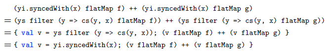
6.3.3 Homomorphism over flatMap
The “homomorphism” equation below is valid for standard collection types, provided expressions e, f, and g have no observable side effects. This equation is the basis for parallelization of flatMap in, for example, Hadoop-like platforms.
A similar homomorphism equation holds for syncedWith. Suppose val yi = new EIterator(us ++ vs, bf, cs) for some us, vs, bf, and cs. Then, after replacing val yi = new EIterator(us ++ vs, bf, cs) by
 $\{\mathtt{val ui = new EIterator(us, bf, cs); val vi = new EIterator(vs, bf, cs)}\}$
, the equation below holds.
$\{\mathtt{val ui = new EIterator(us, bf, cs); val vi = new EIterator(vs, bf, cs)}\}$
, the equation below holds.

This equation follows because

This equation offers a simple way to parallelize syncedWith.
6.4 Possible syntax for Synchrony iterator
Considering the safe-use conditions, it is perhaps pertinent to suggest a syntax for Synchrony iterator that automatically enforces all the safe-use conditions, apart from the safe-use conditions on monotonicity and antimonotonicity. One possibility is to introduce the following generator pattern into comprehension syntax:
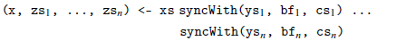
This way, the EIterator class can be hidden from user-programmers, and they can be told that zs
 $_j$
=
$_j$
=
 $\mathtt{ys.filter((y) \Rightarrow cs_j(y, x))}$
at all times in terms of value, as per Proposition 6.2, but is obtained very efficiently.
$\mathtt{ys.filter((y) \Rightarrow cs_j(y, x))}$
at all times in terms of value, as per Proposition 6.2, but is obtained very efficiently.
This generator pattern is compiled by desugaring it to

Usual “deforestation” rules (Wadler Reference Wadler1990) should be able to optimize this further to remove the intermediate collection introduced by this desugaring. If not, the generator pattern can also be desugared into the “chain of generators and assignments” pattern below:

The program mtg4 in Figure 12 is a rewrite of the program mtg3 from Figure 10 using this suggested syntax for Synchrony iterator. As can be seen, using this syntax, the three Synchrony iterators xi, yi, and zi that earlier appeared explicitly in mtg3 are now tucked away from sight. The user-programmer is thus presented with a pure functional comprehension syntax which uses a slightly enhanced generator form. Footnote 11

Fig. 12. The arranging-meeting example revisited again. The program mtg4 is a rewrite of the program mtg3 from Figure 10 using the generator syntax suggested for Synchrony iterator.
7 Some use-cases and a stress test
Synchrony fold and Synchrony iterator for querying relational databases in general, genomic datasets in particular, and timestamped data streams is discussed here. A stress test on using them on genomic datasets is also presented.
7.1 Relational database queries
The use-case of Synchrony fold and Synchrony iterator in the context of relational database querying should be quite clear already. Further technical and theoretical details are given in a companion paper (Wong Reference Wong2021). So, here, we just point out that only one extra function is needed to make all relational database queries (including group-by, order-by, and aggregate functions) efficiently implementable in first-order restricted Scala endowed with Synchrony fold and Synchrony iterator. That extra function is sortWith(f)(xs) which sorts the collection xs: Vec[A] using the ordering function f: (A,A) => Boolean. This is because Synchrony fold and Synchrony iterator require their input to be suitably sorted beforehand.
Actually, sorting at quadratic time complexity is already expressible in first-order restricted Scala endowed with Synchrony fold. Theorem 4.5 implies that all functions defined using first-order restricted Scala with Synchrony fold have time complexity of the form
 $O(m^n)$
where m is input size. Since efficient sorting requires
$O(m^n)$
where m is input size. Since efficient sorting requires
 $\Omega(m \log(m))$
time in general, this means sorting takes
$\Omega(m \log(m))$
time in general, this means sorting takes
 $\Theta(m^2)$
time in first-order-restricted Scala with Synchrony fold. Thus, it is necessary to provide an efficient sortWith sorting function to user-programmers, to ensure that they are able to implement any relational database queries efficiently in this framework.
$\Theta(m^2)$
time in first-order-restricted Scala with Synchrony fold. Thus, it is necessary to provide an efficient sortWith sorting function to user-programmers, to ensure that they are able to implement any relational database queries efficiently in this framework.
It is worth remarking that on-disk sorting is much easier to implement than on-disk indexed tables; cf. Silberschatz et al. (Reference Silberschatz, Korth and Sudarshan2016). It is thus a virtue of Synchrony iterator, which needs only the former when processing very large collections, relative to approaches that try to compile join-expressing comprehensions into indexed tables.
7.2 Genometric queries
A second use-case is genometric queries on genomic datasets. BEDOPS (Neph et al. Reference Neph, Kuehn, Reynolds, Haugen, Thurman, Johnson, Rynes, Maurano, Vierstra, Thomas, Sandstorm, Humbert and Stamatoyannopoulos2012) and GMQL (Masseroli et al. Reference Masseroli, Canakoglu, Pinoli, Kaitoua, Gulino, Horlova, Nanni, Bernasconi, Perna, Stamoulakatou and Ceri2019) are two notable toolkits for processing these datasets and support similar query operations. The former via unix-style commands. The latter via a specialized GenoMetric Query Language. The data model is highly constrained in such domain-specific toolkits. GMQL is used here for illustration, modulo some liberty taken with GMQL’s syntax.
There are only a few main object types. The first main object type is the genomic region; this is Bed(chrom: String, start: Int, end: Int, …) for a region located on chromosome chrom, beginning at position start, ending at position end, plus some other pieces of information which are omitted here. Regions on the same chromosome are ordered by their start and end point lexicographically; regions on different chromosomes are ordered by their chrom value. This ordering
 $<_{\mathtt{Bed}}$
defines the default isBefore predicate on regions, viz. isBefore(y, x) if and only if y
$<_{\mathtt{Bed}}$
defines the default isBefore predicate on regions, viz. isBefore(y, x) if and only if y
 $<_{\mathtt{Bed}}$
x. The next main object is the genome, which is a BED file; it is a large text file in the BED format (Neph et al. Reference Neph, Kuehn, Reynolds, Haugen, Thurman, Johnson, Rynes, Maurano, Vierstra, Thomas, Sandstorm, Humbert and Stamatoyannopoulos2012), the de facto format for this kind of information in the bioinformatics community. A BED file is just a collection of regions, abstracted here as Vec[Bed]. The next main object type is the sample Sample(bedFile: Vec[Bed], meta: …), which is just a BED file and its associated metadata. The last main object is the sample database, which is just a collection of samples; it is abstracted here as Vec[Sample].
$<_{\mathtt{Bed}}$
x. The next main object is the genome, which is a BED file; it is a large text file in the BED format (Neph et al. Reference Neph, Kuehn, Reynolds, Haugen, Thurman, Johnson, Rynes, Maurano, Vierstra, Thomas, Sandstorm, Humbert and Stamatoyannopoulos2012), the de facto format for this kind of information in the bioinformatics community. A BED file is just a collection of regions, abstracted here as Vec[Bed]. The next main object type is the sample Sample(bedFile: Vec[Bed], meta: …), which is just a BED file and its associated metadata. The last main object is the sample database, which is just a collection of samples; it is abstracted here as Vec[Sample].
Queries at the level of samples mainly select samples from the sample database to analyze. Queries at the level of BED files mainly extract and process regions of interest. The first kind of queries is basically simplified relational database queries. The second kind of queries are the specialized ones that a relational database cannot handle efficiently. The reason is that these queries invariably have a join predicate which is a conjunction of “genometric” predicates. The GMQL “genometric” predicates in essence are: DL(n)(y, x), meaning the regions overlap or their nearest points are less than n bases apart; DG(n)(y, x), meaning the regions do not overlap and their nearest points are more than n bases apart; and a few other similar ones. GMQL also implicitly imposes, on genometric predicates, the constraint that y and x are no further apart than a system-fixed number of bases (e.g., 200,000 bases.) For a reader who is unfamiliar with genomics, “bases,” or “bp,” is the unit used for describing distance on a genome.
GMQL queries can be easily modeled and efficiently implemented in our Synchrony iterator framework. Let xs: Vec[Bed] and ys: Vec[Bed] be two BED files sorted in accordance to
 $<_{\mathtt{Bed}}$
. Then, isBefore is monotonic with respect to
$<_{\mathtt{Bed}}$
. Then, isBefore is monotonic with respect to
 $(\mathtt{xs}, \mathtt{ys})$
. Genometric predicates such as DL(n) are antimonotonic with respect to isBefore. Genometric predicates such as GL(n) are not antimonotonic with respect to isBefore. As GMQL automatically inserts DL(200000) as an additional genometric predicate into a query, a query has at least one antimonotonic genometric predicate.
$(\mathtt{xs}, \mathtt{ys})$
. Genometric predicates such as DL(n) are antimonotonic with respect to isBefore. Genometric predicates such as GL(n) are not antimonotonic with respect to isBefore. As GMQL automatically inserts DL(200000) as an additional genometric predicate into a query, a query has at least one antimonotonic genometric predicate.
The implementation of GMQL using Synchrony iterator is described in a companion paper (Perna et al. Reference Perna, Pinoli, Tannen, Ceri and Wong2021). Here, we just briefly describe a more complex GMQL query operator,
 $\mathtt{JOIN(g_1, ..., g_n; f, h, j)(xss, yss)}$
. This GMQL query finds all pairs of samples xs in xss and ys in yss satisfying the join predicate j(xs, ys) on samples. Then for each such pair of samples xs and ys, for each pair of regions x in xs.bedFile and y in ys.bedFile satisfying all the specified genometric predicates
$\mathtt{JOIN(g_1, ..., g_n; f, h, j)(xss, yss)}$
. This GMQL query finds all pairs of samples xs in xss and ys in yss satisfying the join predicate j(xs, ys) on samples. Then for each such pair of samples xs and ys, for each pair of regions x in xs.bedFile and y in ys.bedFile satisfying all the specified genometric predicates
 $\mathtt{g_1(y, x)}$
, …,
$\mathtt{g_1(y, x)}$
, …,
 $\mathtt{g_n(y, x)}$
, it builds a new region f(x, y); these new regions are put into a new BED file xys; finally, a new sample having BED file xys and metadata h(x.meta,y.meta) is produced.
$\mathtt{g_n(y, x)}$
, it builds a new region f(x, y); these new regions are put into a new BED file xys; finally, a new sample having BED file xys and metadata h(x.meta,y.meta) is produced.
![]() is naturally and efficiently embedded into first-order Scala via comprehension syntax and Synchrony iterator. To wit, it is realized by
is naturally and efficiently embedded into first-order Scala via comprehension syntax and Synchrony iterator. To wit, it is realized by
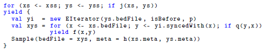
where p is the conjunction of all the antimonotonic predicates among g
 $_1$
…, g
$_1$
…, g
 $_n$
and q is the conjunction of all the remaining predicates among g
$_n$
and q is the conjunction of all the remaining predicates among g
 $_1$
…, g
$_1$
…, g
 $_n$
. In fact, our Synchrony-based GMQL implementation does this decomposition of the list of input genometric predicates into p and q automatically.
$_n$
. In fact, our Synchrony-based GMQL implementation does this decomposition of the list of input genometric predicates into p and q automatically.
7.3 A stress test
We stress-tested Synchrony iterator by re-implementing GMQL using Synchrony iterator. The GMQL engine (Masseroli et al. Reference Masseroli, Canakoglu, Pinoli, Kaitoua, Gulino, Horlova, Nanni, Bernasconi, Perna, Stamoulakatou and Ceri2019) is a state-of-the-art purpose-built system for querying genomic datasets. GMQL is optimized for sample databases containing many samples, with each sample having a large BED file (Neph et al. Reference Neph, Kuehn, Reynolds, Haugen, Thurman, Johnson, Rynes, Maurano, Vierstra, Thomas, Sandstorm, Humbert and Stamatoyannopoulos2012) containing tens of thousands to hundreds of thousands of genomic regions. GMQL achieves high performance by binning the genome into chunks and comparing different bins concurrently (Gulino et al. Reference Gulino, Kaitoua and Ceri2018).
As GMQL is based on Scala, we re-implemented it using Synchrony iterator in Scala; this way, the influence of programming language and compiler differences is eliminated. The Synchrony implementation comes with a sequential mode (samples and their BED files are processed in a strictly sequential manner) and a sample-parallel mode (BED files of different samples are processed in parallel but regions in a BED file are processed in a sequential manner.) This re-implementation comprises circa 4,000 lines of Scala codes as counted by cloc and makes use of some Scala function libraries. In contrast, the original GMQL engine comprises circa 24,000 lines of Scala codes and uses more Scala function libraries and also Spark function libraries. This comparison reveals the merit of Synchrony iterator in enabling complex algorithms to be expressed in a succinct high-level manner.
For benchmarking, we deployed the GMQL engine on a local installation of Apache Spark, which simulates a small cluster on a single multicore machine. We refer to this as the GMQL command-line interface, or CLI. The machine is a laptop with 2.6 GHz 6-Core i7, 16 GB 2667 MHz DDR4, 500 GB SSD. Despite the simplicity of our implementation, it significantly outperforms GMQL CLI on essentially all test queries and on the full range of dataset sizes and equals GMQL CLI on the largest-size datasets. This is a strong testimony to Synchrony iterator as an elegant idea for expressing efficient synchronized iterations on multiple collections in a succinct and easy-to-understand manner. The implementation and detailed evaluation are presented in a companion paper (Perna et al. Reference Perna, Pinoli, Tannen, Ceri and Wong2021). The implementation is available at https://www.comp.nus.edu.sg/~wongls/projects/synchrony.
We present below some comparison results on a simple region MAP query. The GMQL MAP query takes two sample databases xss and yss and produces for each pair of BED files xs.bedFile in xss and ys.bedFile in yss, and each region x in xs.bedFile, the number of regions in ys.bedFile that it overlaps with. GMQL executes its MAP operator in a four-level deeply nested loop, in a brute-force parallel manner; that is, all BED file pairs are analyzed in parallel. For each BED file pair, the BED files are chopped into bins; the bins are paired; and all bin pairs are analyzed in parallel. Ignoring parallelism, the complexity is
 $O(n^2 m^2)$
assuming both xss and yss contain n BED files and each BED file contains
$O(n^2 m^2)$
assuming both xss and yss contain n BED files and each BED file contains
 $m >> n$
regions. The Synchrony iterator version uses a two-level nested loop to pair up the BED files, but each pair of BED files is analyzed using a Synchrony iterator:
$m >> n$
regions. The Synchrony iterator version uses a two-level nested loop to pair up the BED files, but each pair of BED files is analyzed using a Synchrony iterator:

The sample-parallel version runs the two-level nested loop in parallel but the Synchrony iterator sequentially. The sequential version does everything sequentially. Ignoring parallelism, the complexity is
 $O((2k + 1) m n^2)$
where k is a small number corresponding to the maximum number of overlaps a region can have with other regions.
$O((2k + 1) m n^2)$
where k is a small number corresponding to the maximum number of overlaps a region can have with other regions.
For this paper, the three versions are run on three input settings (SB, MB, BB) containing varying number of BED files, where each BED file has 100,000 regions. The setting SB means both xss and yss contain exactly one BED file; thus, there is exactly one BED file pair to analyze. The setting MB means both xss and yss contain exactly ten BED files; thus, there are 100 BED file pairs to analyze. The setting BB means both xss and yss contain exactly one hundred BED files; thus, there are 10,000 BED file pairs to analyze. Roughly, xss and yss are each of size circa 10MB, 96MB, and 696MB on disk in settings SB, MB, and BB. The timings are shown in Figure 13. It is clear that the two Synchrony iterator versions are far more efficient than GMQL CLI. Only in the BB setting, GMQL CLI is able to beat the strict sequential Synchrony iterator. But GMQL CLI’s brute-force parallelism is still no match to sample-parallel Synchrony iterator for these and other settings considered.

Fig. 13. Performance of GMQL CLI and Synchrony emulation on simple region MAP. Time in seconds, average of 30 runs for SB and MB, and 5 runs for BB. Purple: GMQL CLI. Blue: Sequential Synchrony emulation. Green: Sample-parallel Synchrony emulation.
7.4 Stream queries
As a last use-case, we model timestamped data streams. Two kinds of objects are considered for this purpose. The first kind is called observations. An observation x: Obs(at: Int, id: …) has a timestamp x.at, which is the time the observation is obtained, and has some other pieces of information that are irrelevant for our purpose. All timestamps are the number of nanoseconds that have elapsed since a fixed reference time point. The second kind is called observation streams. An observation stream is just a collection of observations, xs: Vec[Obs].
Observations are intrinsically ordered by their timestamps. Thus, it is natural to define the following as the isBefore predicate on observation streams:
bf(y, x) = y.at < x.at
and it is also natural to assume that observation streams are sorted by timestamps by default. A variety of canSee predicates can be easily defined, such as:
notAfter(y, x) = ! (y.at > x.at)
within(n)(y, x) = abs(y.at - x.at) <= n
For convenience, let clk be a stream of observations representing regular clock ticks at intervals of 1 ms. Also, let xss, yss, and zss be several streams of observations. Then, a variety of observation processing can be easily and efficiently expressed. Just for practice, to see how it looks, the suggested syntax for abstracting away Synchrony iterator from Section 6.4 is used here; the programs below are not legitimate Scala.
-
cartesian(f)(clk, xss, yss, zss) group observations in xss, yss, and zss into 1 ms time-synchronized blocks applies f to each block to generate a new observation stream.
-
mostRecent(f)(clk, xss, yss, zss) applies f to the last observation in xss, yss, and zss within each 1 ms block. Skips a block if any stream contains no observation in that block of time.
-
affineMostRecent(f)(clk, xss, yss, zss) applies f to the last observation in xss, yss, and zss within each 1 ms block. If a block has a stream which contains no observation in this block of time, keep observations in this block and consider them with the next block.


As can be seen, a variety of temporal stream processing and synchronization operators, akin to those in Bracevac et al. (Reference Bracevac, Amin, Salvaneschi, Erdweg, Eugster and Mezini2018), can be implemented in comprehension syntax using Synchrony iterator. Notably, provided there are not too many events within each 1 ms block and f has at most linear-time complexity, all of these examples have linear-time complexity. If the observation type has a structure that carries more information (e.g., length of observation, if observation extends over a period of time), an even richer variety of antimonotonic predicates can be defined and used in specifying stream synchronization.
To some extent, this use-case illustrates that Synchrony iterator is not restricted to database query processing. Rather, it is capturing and generalizing common patterns and forms of synchronized iterations, such as those found in database query processing and in stream event processing.
8 Other possibilities
8.1 Grouping
It is instructive to look at the function groups in the top half of Figure 14. It was suggested by a reviewer as an approach to efficient implementation of relational joins. The idea is based on grouping. This suggestion inspired us to introduce the Synchrony generator syncGenGrp, which we did not describe in the initial draft of this paper mainly because it returns a nested collection and thus, strictly speaking, does not meet the first-order restriction requirement.

Fig. 14. Alternative attempts to define syncGenGrp. The function groups is only correct when cs is an equijoin predicate. The function groups2 is equivalent to syncGenGrp and has comparable efficiency.
The reviewer probably had in mind a function like syncGenGrp and provided the function groups in Figure 14 as the implementation. However, this only works correctly when the join predicate cs is a conjunction of equality tests, i.e., an equijoin. Here is an example to show that it does not correctly implement a join in general. Let us regard xs: Vec[Event] and ys: Vec[Event] as lists of line segments sorted by
 $(\mathtt{start}, \mathtt{end})$
. Consider the following line segments.
$(\mathtt{start}, \mathtt{end})$
. Consider the following line segments.
-
a = Event(start = 10, end = 70, id = “a”)
-
b = Event(start = 20, end = 30, id = “b”)
-
c = Event(start = 40, end = 80, id = “c”)
-
d = Event(start = 60, end = 90, id = “d”)
Let isBefore and overlap be as defined in Figure 1. Let xs be a singleton containing the line segment d and ys comprises the line segments a, b, and c in this order. Then, ov1(xs, ys) evaluates to exactly the two pairs (d, a) and (d, c). In agreement with ov1(xs, ys), syncGenGrp(isBefore, overlap)(xs, ys) evaluates to the singleton (d, Vec(a, c)). However, groups(isBefore, overlap)(xs, ys) incorrectly evaluates to an empty collection.
Perhaps instead of val yt = ys.dropWhile(y => bf(y, x)), the reviewer meant val yt = ys.dropWhile(y => bf(y, x) && !cs(y, x)). This revised groups(bf, cs)(xs, ys) works correctly when bf is monotonic with respect to
 $(\mathtt{xs}, \mathtt{ys})$
and cs is reflexive and convex with respect to bf. It does not work as expected when cs is antimonotonic but not convex. We mentioned earlier that predicates which are reflexive and convex are also antimonotonic and that the converse is not true. The overlap predicate on events is such an example; it is antimonotonic but not convex. This can be seen using the line segments given above: overlap(a, d) and overlap(c, d) but not overlap(b, d). Indeed, this revised groups function returns the singleton (d, Vec(a)), which is still incorrect.
$(\mathtt{xs}, \mathtt{ys})$
and cs is reflexive and convex with respect to bf. It does not work as expected when cs is antimonotonic but not convex. We mentioned earlier that predicates which are reflexive and convex are also antimonotonic and that the converse is not true. The overlap predicate on events is such an example; it is antimonotonic but not convex. This can be seen using the line segments given above: overlap(a, d) and overlap(c, d) but not overlap(b, d). Indeed, this revised groups function returns the singleton (d, Vec(a)), which is still incorrect.
In order to get the correct semantics as syncGenGrp, the definition of groups must be modified to account for antimonotonicity. This can be done as in groups2, depicted in the bottom half of Figure 14. In groups2, for each x in xs, step iterates on the current copy of ys, to divide it using takeWhile and dropWhile. The function dropWhile stops the iteration on ys as soon as an item y in ys is encountered such that both bf(y, x) and cs(y, x) are false and yields the remainder nos. This early stopping is correct due to Antimonotonicity Condition 2. The function takeWhile copies items on ys until an item y in ys is encountered such that both bf(y, x) and cs(y, x) are false, obtaining the prefix maybes. Those items in maybes that can see x are extracted into yes and returned as the result for this x. The function step also updates ys to yes ++: nos, “rewinding” it and setting it up for the next item in xs. Thus, for the next x, the iteration on ys effectively skips over all the items in ys that are before it and cannot see it. This skipping is correct due to Antimonotonicity Condition 1.
Group2 and syncGenGrp can be shown to define the same function and have similar time complexity, albeit group2 is slightly less efficient than syncGenGrp. The concepts of monotonicity and antimonotonicity seem fundamental to achieving efficient synchronized iteration. In particular, groups2 needs both of these to ensure correctness. Their use in groups2 has further clarified how these concepts interact to synchronize iteration. Specifically, synchronized iteration on two collections, which are already sorted in a comparable ordering, is characterized by knowing precisely when to start, stop, and “rewind.” Hence, by explicitly parameterizing its iteration control on monotonicity and antimonotonicity, Synchrony fold can perhaps be regarded as a programming construct that characterizes efficient synchronized iteration on ordered collections.
8.2 Indexed tables
A reviewer also introduced us to the recent works of Gibbons (Reference Gibbons2016) and Gibbons et al. (Reference Gibbons, Henglein, Hinze and Wu2018), which investigate programming language embedding of joins that avoid naive evaluation strategies. These works provide an elegant mathematical foundation for indexing and grouping, leading to efficient implementation of equijoins. Underlying the theoretical perspective of these works is the use of indexed tables.
Indexed tables are part of the repertoire of collection-type libraries of modern programming languages. For example, the collection-type libraries of Scala provide a groupBy method. For a collection ys: Vec[A], and an indexing function f: A => K, ys.groupBy(f) builds and returns an indexed table ms: Map[K,Vec[A]], where ms(ky) is the precomputed result of for (y <- ys; if f(y) == ky) yield y. If f is a function of O(1) time complexity, the indexed table is constructed in
 $O(|\mathtt{ys}|)$
time and accessing ms(f(y)) takes O(1) time.
$O(|\mathtt{ys}|)$
time and accessing ms(f(y)) takes O(1) time.
This groupBy function is useful for implementing efficient equijoin by a user-programmer, if we disregard the fact that it returns a nested collection and is thus not first order. For a direct example, assuming f and g are constant time functions, the equijoin for (x <- xs; y <- ys; if g(x) == f(y)) yield (x, y) can be computed in
 $O(|\mathtt{xs}| + |\mathtt{ys}|)$
time using an indexed table as
$O(|\mathtt{xs}| + |\mathtt{ys}|)$
time using an indexed table as
 $\mathtt{\{ val ms = ys.groupBy(f); for x \leftarrow xs; y \leftarrow ms(g(x)) yield (x,y)\}}$
. This corresponds to an index-seek join strategy, which a database system usually uses when it expects there are not many y that matches any x at all. As another example, Gibbons (Reference Gibbons2016) describes an interesting perspective where collections are viewed as indexed tables and derives a zip-parallel comprehension for joining them. This strategy corresponds to the index-scan join strategy, which a database system uses when it expects most x matches at least one y and vice versa.
$\mathtt{\{ val ms = ys.groupBy(f); for x \leftarrow xs; y \leftarrow ms(g(x)) yield (x,y)\}}$
. This corresponds to an index-seek join strategy, which a database system usually uses when it expects there are not many y that matches any x at all. As another example, Gibbons (Reference Gibbons2016) describes an interesting perspective where collections are viewed as indexed tables and derives a zip-parallel comprehension for joining them. This strategy corresponds to the index-scan join strategy, which a database system uses when it expects most x matches at least one y and vice versa.
Using an indexed-table approach to implement an equijoin has a key advantage that the input collections do not need to be sorted to begin with. Provided all indexed tables which are needed can fit into memory, implementing an equijoin using an indexed-table approach is superior to using Synchrony iterator. If one or more of the input collections are unsorted or are in some unsuitable orderings, these inputs have to be sorted before Synchrony iterator can be used to process them; this can be a significant overhead when the input collections which require sorting are large.
On the other hand, there are several limitations with indexed tables, especially when we are not operating on an actual database system. Firstly, this means the indexed table is an in-memory structure; so, it is not suitable for very large collections. Footnote 12 Secondly, the indexed table has to be completely constructed before it is used; so, it is not suitable for data streams. Lastly, and crucially, as an indexed table relies on exact equality to directly retrieve entries, it can easily implement efficient equijoin but it cannot implement non-equijoin such as band join and interval join.
In contrast, Synchrony iterator does not suffer these limitations. In other words, Synchrony iterator is a more general and more uniform approach for realizing efficient equijoin and a large class of non-equijoin. Synchrony iterator is thus justifiably appealing.
9 Concluding remarks
Modern programming languages typically provide some form of comprehension syntax for manipulating collection types. In this regard, comprehension syntax does not add extensional expressive power, but it makes programs much more readable (Trinder Reference Trinder1991; Buneman et al. Reference Buneman, Libkin, Suciu, Tannen and Wong1994). Comprehensions typically correspond to nested loops. So, it is difficult to use comprehension syntax to express efficient algorithms for, for example, database joins. This has partly motivated developments that introduced alternative binding semantics for comprehension syntax, so that some comprehensions are not compiled into nested loops. For example, parallel and grouping comprehension were introduced to enable implementation of efficient database queries in the style of comprehension syntax (Wadler & Peyton Jones Reference Wadler and Peyton Jones2007; Gibbons Reference Gibbons2016; Gibbons et al. Reference Gibbons, Henglein, Hinze and Wu2018). Nonetheless, it has not been formally demonstrated that efficient algorithms for, for example, equijoin cannot be implemented without making such refinements to comprehension syntax.
The first contribution of this paper is to highlight, in a precise sense, comprehension syntax suffers a limited-mixing handicap. In particular, this formally confirms that efficient algorithms for low-selectivity database joins—and this includes equijoin—cannot be implemented using comprehension syntax in the first-order setting (i.e., first-order restricted Scala in the context of this paper.) This justifies, from the intensional expressive power point of view, that these interesting works are necessary.
Although there is no efficient implementation for low-selectivity database joins in the first-order setting, they are nonetheless expressible as functions in the first-order setting. Therefore, the gap is purely in the intensional expressive power of comprehension syntax. So, we considered whether any function commonly provided in the collection-type libraries of modern programming languages is able to fix this gap. The limited-mixing handicap of comprehension syntax in the first-order setting remains even after adding any one of foldLeft, takeWhile, dropWhile, and zip, and most common functions in these libraries are derivatives of foldLeft.
The second contribution of this paper is to identify and propose a candidate library function which fills this gap. We noticed that, apart from zip, the notion of general synchronized iteration on multiple collections is conspicuously absent from current collection-type libraries. Hence, to kill two birds with one stone, we looked for a function that encapsulates a common pattern of general synchronized iteration on multiple collection. Arguably, foldLeft is the most powerful function in collection-type libraries of modern programming languages, as most other commonly found functions in these libraries are extensionally expressible using foldLeft. So, as an upperbound, we identified Synchrony fold, which is a novel synchronized iteration function that expresses the same functions as foldLeft in the first-order setting and yet expresses more algorithms, including efficient low-selectivity database joins. Furthermore, just as a simple restriction can be imposed on foldLeft to cut its extensional expressive power to precisely match comprehension syntax, a similar restriction can be imposed on Synchrony fold to cut its extensional expressive power to precisely match comprehension syntax. This restricted form is Synchrony generator. Synchrony generator expresses exactly the same functions as comprehension syntax in the first-order setting, but it expresses a richer repertoire of algorithms, including efficient low-selectivity database joins. Hence, Synchrony generator is a conservative extension of comprehension syntax that precisely fills its intensional expressiveness gap.
Synchrony generator is nonetheless not well dovetailed with comprehension syntax in the first-order setting. In particular, synchronized iteration over multiple ordered collections simultaneously apparently can only be expressed using Synchrony generator in an esthetically clumsy manner in the first-order setting. When a function zip
 $_n$
for simultaneously zipping n collections is available, efficient synchronized iteration over n collections can be succinctly and elegantly expressed using Synchrony generator and this function. However, zip
$_n$
for simultaneously zipping n collections is available, efficient synchronized iteration over n collections can be succinctly and elegantly expressed using Synchrony generator and this function. However, zip
 $_n$
is outside the first-order setting. Moreover, this approach carries overheads of n extra scans of at least one dataset. Another limitation of this approach is that it is not user-programmer friendly: A zoo of zip
$_n$
is outside the first-order setting. Moreover, this approach carries overheads of n extra scans of at least one dataset. Another limitation of this approach is that it is not user-programmer friendly: A zoo of zip
 $_3$
, zip
$_3$
, zip
 $_4$
, etc. have to be provided.
$_4$
, etc. have to be provided.
The third contribution of this paper is Synchrony iterator. We found that Synchrony generator is algorithmically equivalent to iterating on the items in a first collection, and invoking Synchrony iterator on each of these items to efficiently return matching items in a second collection. Synchrony iterator thus smoothly dovetails with comprehension syntax. More importantly, it enables efficient synchronized iteration on multiple collections to be simply expressed in comprehension syntax in a first-order setting and without the n extra-scan overheads.
Synchrony fold, Synchrony generator, and Synchrony iterator can be regarded as capturing an intuitive pattern of efficient synchronized iteration on ordered collections. They suggest that efficient synchronized iteration on ordered collections are characterized by a monotonic isBefore predicate that relates the orderings of the input collections, and an antimonotonic canSee predicate that identifies matching pairs to act on. The antimonotonicity conditions on canSee further inform that the efficiency of the synchronization arises from exploiting “right-sided convexity” of the matching items. Indeed, together, these predicates make explicit where to start, stop, and rewind an iteration on two collections, thereby achieving efficient synchronization.
The fourth contribution of this paper is the revelation that efficient synchronized iteration on ordered collections is captured by such a pattern which is characterized by the monotonic isBefore and antimonotonic canSee predicates. A corollary of this fourth contribution is the result that Synchrony generator (and thus Synchrony iterator) is a natural generalization of the merge join algorithm (Blasgen & Eswaran Reference Blasgen and Eswaran1977; Mishra & Eich Reference Mishra and Eich1992) widely used in database systems for decades for realizing efficient equijoins. With a simple modification implied by Synchrony generator, the modified merge join algorithm can work as long as the join predicate is antimonotonic with respect to the sort order of the relations being joined.
Lastly, we briefly described using Synchrony iterator to re-implement GMQL (Masseroli et al. Reference Masseroli, Canakoglu, Pinoli, Kaitoua, Gulino, Horlova, Nanni, Bernasconi, Perna, Stamoulakatou and Ceri2019), which is a state-of-the-art query system for large genomic datasets. The Synchrony-based re-implementation is more efficient than GMQL and is also six-fold shorter in terms of number of lines of codes, thereby validating the theory and design of Synchrony fold and Synchrony iterator.
This paper primarily illustrates Synchrony fold, Synchrony generator, and Synchrony iterator using examples based on low-selectivity database joins. Nonetheless, Section 7.4 briefly showcases using Synchrony iterator to specify event stream processing operators. This suggests Synchrony fold and Synchrony iterator capture patterns of efficient synchronized iteration, showing that they can be parameterized by a pair of monotonic isBefore and antimonotonic canSee predicates. However, our notion of synchronized iteration, as encapsulated by Synchrony fold, generator, and iterator, is quite constrained. It maybe a worthwhile future work to understand what interesting yet common patterns of efficient synchronized iteration are not encapsulated by Synchrony fold and Synchrony iterator.
Conflicts of Interest
None
Acknowledgments
Stefano Ceri invited us to the GeCo Workshop on Challenges in Data-Driven Genomic Computing, held in Como, Italy, in March 2019. This work evolved from the talk given by LW at the workshop and the ensuing interesting discussions with VT and SP. We thank Stefano for his invitation and surreptitious seeding of this work. Jeremy Gibbons and the reviewers provided very useful suggestions on this paper. They also brought many relevant works and ideas to our attention. Their comments greatly enriched our perspective in this work. We thank them for their invaluable contribution in helping us improve this work. SP and LW were supported by National Research Foundation, Singapore, under its Synthetic Biology Research and Development Programme (Award No: SBP-P3), and by Ministry of Education, Singapore, Academic Research Fund Tier-1 (Award No: MOE T1 251RES1725) and Tier-2 (Award No: MOE-T2EP20221-0005). In addition, VT was supported in part by a Kwan Im Thong Hood Cho Temple Visiting Professorship, and LW was supported in part by a Kwan Im Thong Hood Cho Temple Chair Professorship. Any opinions, findings, and recommendations expressed herein are those of the authors and do not reflect the views of these grantors.


 Open access
Discussions
No Discussions have been published for this article.