


1. Introductionc
The COVID-19 pandemic (The Novel Coronavirus Pneumonia Emergency Response Epidemiology Team, 2020) creates the need to allow for mortality shocks in experience analysis performed by actuaries. The intense nature of the repeated COVID-19 mortality shocks in many countries means that traditional methods based around annual
 ${q_x}$
-style mortality rates are inadequate: mixing periods of shock and non-shock mortality understates the true intensity of mortality spikes. Furthermore, mortality shocks in the experience data may lead to bias in bases for reserving and pricing. A continuous-time methodology that copes with sharp fluctuations in time is required.
${q_x}$
-style mortality rates are inadequate: mixing periods of shock and non-shock mortality understates the true intensity of mortality spikes. Furthermore, mortality shocks in the experience data may lead to bias in bases for reserving and pricing. A continuous-time methodology that copes with sharp fluctuations in time is required.
This paper covers the modelling and analysis of portfolio experience data only. The subject of future mortality trends is out of scope, although section 9 briefly considers the topic of year-on-year improvements. In our models, we make extensive use of splines, which are flexible mathematical functions. There are numerous different kinds of spline, each with different properties and thus suitable for different purposes. In this paper, we use two kinds of spline: Hermite splines, which span the interval [0,1], and Schoenberg (Reference Schoenberg1964) splines, which are piecewise local polynomials on the real line. In modern literature, such as de Boor (Reference de Boor2001) and Eilers & Marx (Reference Eilers and Marx2021), references to B-splines are synonymous with Schoenberg splines. Since this paper uses two different kinds of spline, we use the term Schoenberg spline, rather than B-spline, to distinguish from Hermite splines.
Past mortality modelling using splines in calendar time, such as Currie et al. (Reference Currie, Durban and Eilers2006) and Eilers et al. (Reference Eilers, Gampe, Marx and Rau2008), uses stratified grouped counts. In contrast, we use individual records in a survival model so that we can include covariates like gender, pension size and other factors typically available to actuaries. We use Hermite splines to model age- and income-related mortality and we use Schoenberg (Reference Schoenberg1964) splines to model mortality in time. Here, we compress the knot spacing for splines in time to half a year or less to model sharp swings in mortality.
The plan of the rest of this paper is as follows: section 2 presents important features of COVID-19 mortality in the UK and the resulting need for continuous time methods in place of annual
 ${q_x}$
rates; section 3 describes the data set used in the paper; section 4 describes the use of Hermite splines for modelling mortality by age, while section 5 describes how to use Hermite splines for modelling mortality by annuity amount. Section 6 recaps the application of Schoenberg splines for modelling mortality levels over time. Section 7 considers the ability of the method to identify seasonal variation, while section 8 looks at the additional requirements for modelling the COVID-19 mortality shocks in the UK. Section 9 looks at further insights that can be derived, such as portfolio-specific improvement rates. Section 10 considers the use of the methodology to allow for the impact of occurred-but-not-reported (OBNR) deaths. Section 11 considers the conditions under which Schoenberg (Reference Schoenberg1964) splines may – and may not – be used for mortality patterns by age. Section 12 discusses the use and limitations of information criteria, and the role of actuarial judgement in selecting models. Section 13 concludes.
${q_x}$
rates; section 3 describes the data set used in the paper; section 4 describes the use of Hermite splines for modelling mortality by age, while section 5 describes how to use Hermite splines for modelling mortality by annuity amount. Section 6 recaps the application of Schoenberg splines for modelling mortality levels over time. Section 7 considers the ability of the method to identify seasonal variation, while section 8 looks at the additional requirements for modelling the COVID-19 mortality shocks in the UK. Section 9 looks at further insights that can be derived, such as portfolio-specific improvement rates. Section 10 considers the use of the methodology to allow for the impact of occurred-but-not-reported (OBNR) deaths. Section 11 considers the conditions under which Schoenberg (Reference Schoenberg1964) splines may – and may not – be used for mortality patterns by age. Section 12 discusses the use and limitations of information criteria, and the role of actuarial judgement in selecting models. Section 13 concludes.
2. COVID-19 and Other Mortality Shocks
COVID-19 is a new viral disease whose arrival in the UK in 2020 caused deaths to surge to levels not seen since the global influenza pandemic of 1918–1920 (Spreeuwenberg et al., Reference Spreeuwenberg, Kroneman and Paget2018). Figure 1 shows that England & Wales had sharply higher numbers of deaths in 1918 and 2020 compared to preceding years.

Figure 1. Numbers of deaths in England & Wales (
 $ \bullet $
, left scale) with 1918 and 2020 counts circled. The population size is also shown in grey (right scale). Source: ONS.
$ \bullet $
, left scale) with 1918 and 2020 counts circled. The population size is also shown in grey (right scale). Source: ONS.
In many places, the 1918–1920 influenza pandemic appeared as a series of three spikes in mortality, as shown in Figure 2 for Scotland, where the second and third spikes were the most severe. As with influenza in 1918–1920, a key feature of COVID-19 mortality in many countries is that it too takes the form of relatively sharp peaks. These peaks are a result of accelerating infection, followed by changes in health policy and behaviour causing infections to fall. For example, without the lockdown in England on 26 March 2020 (Public Health England, 2020), the first COVID-19 peak would have been higher (and if the lockdown had been declared earlier, the peak would likely have been lower). At the time of writing, there have been two such peaks in the UK, as shown in Figure 3. These peaks form and subside over a period of weeks or months, and an annualised approach to mortality will understate such mortality surges. For this reason, it is important to use continuous time methods like the mortality hazard,
 ${\mu _x}$
, rather than annual
${\mu _x}$
, rather than annual
 ${q_x}$
-style rates.
${q_x}$
-style rates.

Figure 2. Weekly deaths in Scotland in 1918–1919 as percentage of 1913–1917 average. Source: Craufurd Dunlop and Watt (Reference Craufurd Dunlop and Watt1915, Reference Craufurd Dunlop and Watt1916a, Reference Craufurd Dunlop and Watt1916b, Reference Craufurd Dunlop and Watt1918, Reference Craufurd Dunlop and Watt1919, Reference Craufurd Dunlop and Watt1920a, Reference Craufurd Dunlop and Watt1920b).

Figure 3. Daily deaths in UK where the death certificate mentions COVID-19 as one of the causes. Note that the first lockdown legally commenced in England on 26 March 2020. Source: ONS (2021).
COVID-19 made its presence felt in the mortality of annuity portfolios and pension schemes in many countries; Richards (Reference Richards2021b) demonstrated this for annuity portfolios in France, the UK and the USA. COVID-19 therefore creates a problem for actuaries analysing experience data to set bases: the extra mortality of 2020–2021 risks either under-reserving (in the case of liabilities already on the balance sheet) or under-pricing (in the case of insurers writing bulk annuities and longevity swaps). Unfortunately, portfolio administrators seldom record the cause of death, so data like Figure 3 are typically unavailable. Excluding periods of COVID-affected data is also an unsatisfactory approach – pension schemes looking to transact bulk annuities or longevity swaps may only have experience data for the most recent 3–5 years, and discarding one or more of those years’ data is an unaffordable luxury for a pricing actuary. Actuaries therefore require a methodology that works with all-cause mortality data, but which flexibly tracks mortality levels over time to allow for COVID-19 spikes. This way all available experience data can be used, and the actuary can then exercise judgement as to what point in time is most representative for calibrating a mortality basis.
3. Data Description
The data used in this paper comprise individual records from a mature annuity portfolio of the UK insurer. At the end of June 2021, a direct extract was made from the administration systems, as recommended by Macdonald et al. (Reference Macdonald, Richards and Currie2018, section 2.2) to get the most up-to-date data. Policy records were validated using the checks described in Macdonald et al. (Reference Macdonald, Richards and Currie2018, sections 2.3 and 2.4).
Insurer annuity portfolios often contain two or more policies per person, and so deduplication is required for the independence assumption that underpins statistical modelling; see Macdonald et al. (Reference Macdonald, Richards and Currie2018, section 2.5) for discussion of various approaches to deduplication. As is common for UK annuity portfolios, there are many such duplicates – of 351,947 records passing validation, 124,420 records were found to be someone’s second or third annuity, and there were 3 people with 29 annuities each. The tendency to have multiple annuities is correlated with wealth and socio-economic status, so deduplication is an essential step in building a statistical model for actuarial purposes. There were 729 annuities where the annuitant was marked alive on one annuity and dead on another; these annuities were excluded from the data for modelling.
The data set used in this paper is an updated extract of the UK3 data set in Richards (Reference Richards2021b). In this paper, we will continue to refer to it as UK3 for continuity.
4. Hermite Splines for Mortality by Age
A basis of Hermite splines in one dimension (Kreyszig, Reference Kreyszig1999, p. 868) is a collection of four cubic polynomial functions, as shown in Figure 4. A basis of cubic Hermite splines will produce the same fitted curve as a basis of cubic Bézier curves or Bernstein polynomials of degree 3, albeit with different coefficients.

Figure 4. Four Hermite basis splines for
 $u \in [0,1]$
. Note that various potentially useful equalities exist, such as
$u \in [0,1]$
. Note that various potentially useful equalities exist, such as
 ${h_{00}}(u) + {h_{01}}(u) = 1$
and
${h_{00}}(u) + {h_{01}}(u) = 1$
and
 ${h_{10}}(u) + {h_{11}}(1 - u) = 0$
.
${h_{10}}(u) + {h_{11}}(1 - u) = 0$
.
Richards (Reference Richards2020) proposed using Hermite splines for modelling mortality by mapping an age range
 $[{x_0},{x_1}]$
onto
$[{x_0},{x_1}]$
onto
 $[0,1]$
and forming the log hazard as a linear combination of the spline functions in Figure 4. The model for the mortality hazard at age x,
$[0,1]$
and forming the log hazard as a linear combination of the spline functions in Figure 4. The model for the mortality hazard at age x,
 ${\mu _x}$
, is given in equation (1):
${\mu _x}$
, is given in equation (1):
 $$\log \mu _{x} \, = \alpha h_{00}(u) + \omega h_{01}(u) + m_0h_{10}(u) + m_{1} h_{11}(u) $$
 $$u{\mkern 1mu} = {{x - {x_0}} \over {{x_1} - {x_0}}}$$
where the intermediate variable u maps age
 $x \in [{x_0},{x_1}]$
onto
$x \in [{x_0},{x_1}]$
onto
 $[0,1]$
and
$[0,1]$
and
 $\alpha $
,
$\alpha $
,
 $\omega $
,
$\omega $
,
 ${m_0}$
and
${m_0}$
and
 ${m_1}$
are parameters to be estimated. In practice, the
${m_1}$
are parameters to be estimated. In practice, the
 ${h_{11}}$
spline is seldom needed for mortality work and so we often set
${h_{11}}$
spline is seldom needed for mortality work and so we often set
 ${m_1} = 0$
. Doing so forces the mortality hazard in equation (1) to be monotonic at advanced ages, a topic we will return to in section 11. We can further set
${m_1} = 0$
. Doing so forces the mortality hazard in equation (1) to be monotonic at advanced ages, a topic we will return to in section 11. We can further set
 ${m_0} = 0$
to obtain a simple two-parameter alternative to the Gompertz (Reference Gompertz1825) model that is strictly monotonic at all ages, as per equation (2):
${m_0} = 0$
to obtain a simple two-parameter alternative to the Gompertz (Reference Gompertz1825) model that is strictly monotonic at all ages, as per equation (2):
 $$\log {\mu _x} = \alpha {h_{00}}(u) + \omega {h_{01}}(u)$$
Actuarial survival data are typically left-truncated; see Macdonald et al. (Reference Macdonald, Richards and Currie2018, section 1.9) for a discussion of the differences between actuarial survival models and those in medical research, such as described by Collett (Reference Collett2003). To fit a survival model for n individual lifetimes, we use the log-likelihood,
 $\ell $
, in equation (3):
$\ell $
, in equation (3):
 $$\matrix{ \ell \hfill \,{ = - \sum\limits_{i = 1}^n {H_{{x_i}}}({t_i}) + \sum\limits_{i = 1}^n {d_i}\log {\mu _{{x_i} + {t_i}}}} \hfill \cr \hskip-22pt{{H_{{x_i}}}({t_i})} \,{ = \int_0^{{t_i}} {\mu _{{x_i} + s}}ds} \hfill \cr } $$
where
 ${x_i}$
is the exact age when life
${x_i}$
is the exact age when life
 $i = 1, \ldots ,n$
enters observation,
$i = 1, \ldots ,n$
enters observation,
 ${t_i}$
is the time in years that life i is observed and
${t_i}$
is the time in years that life i is observed and
 ${d_i}$
is an indicator variable taking the value 1 if life i is dead at age
${d_i}$
is an indicator variable taking the value 1 if life i is dead at age
 ${x_i} + {t_i}$
and 0 otherwise;
${x_i} + {t_i}$
and 0 otherwise;
 ${H_{{x_i}}}({t_i})$
is the integrated hazard function. The log-likelihood in equation (3) is maximised to find the maximum-likelihood estimates of the parameters underlying
${H_{{x_i}}}({t_i})$
is the integrated hazard function. The log-likelihood in equation (3) is maximised to find the maximum-likelihood estimates of the parameters underlying
 ${\mu _x}$
; see Appendix 14 for the technical details of implementation and model-fitting.
${\mu _x}$
; see Appendix 14 for the technical details of implementation and model-fitting.
Figure 5(a) shows the simplified Hermite spline model of equation (2) fitted to the UK3 data set. Figure 5(b) shows the deviance residuals (McCullagh & Nelder, Reference McCullagh and Nelder1989, p. 39), indicating that Hermite splines are an effective approach to modelling post-retirement mortality, especially where the linear assumption of Gompertz (Reference Gompertz1825) does not hold.

Figure 5. (a) Crude mortality hazard (
 $ \circ $
) for UK3 data set with fitted curve from equation (2). (b) Deviance residuals (
$ \circ $
) for UK3 data set with fitted curve from equation (2). (b) Deviance residuals (
 $ \bullet $
) from the model fit with dashed lines showing the 95% confidence limits for N(0,1) variates. Data cover ages 55–105 years across the period 2015–2020.
$ \bullet $
) from the model fit with dashed lines showing the 95% confidence limits for N(0,1) variates. Data cover ages 55–105 years across the period 2015–2020.
Figure 5 shows that equation (2) does an acceptable job of explaining mortality variation by age. We therefore extend equation (2) to include gender as a risk factor as shown in equation (4), where
 ${z_{i,{\rm{female}}}}$
is an indicator variable taking the value 1 if the annuitant is female and 0 if male.
${z_{i,{\rm{female}}}}$
is an indicator variable taking the value 1 if the annuitant is female and 0 if male.
 ${\alpha _0}$
,
${\alpha _0}$
,
 ${\alpha _{{\rm{female}}}}$
,
${\alpha _{{\rm{female}}}}$
,
 ${\omega _0}$
and
${\omega _0}$
and
 ${\omega _{{\rm{female}}}}$
are parameters estimated by maximum likelihood using equation (3).
${\omega _{{\rm{female}}}}$
are parameters estimated by maximum likelihood using equation (3).
 $$\matrix{ {\log {\mu _{{x_i}}}} \hfill { = {\alpha _i}{h_{00}}(u) + {\omega _i}{h_{01}}(u)} \hfill \cr \hskip19pt{{\alpha _i}} { = {\alpha _0} + {\alpha _{{\rm{female}}}}{z_{i,{\rm{female}}}}} \hfill \cr \hskip19pt{{\omega _i}} { = {\omega _0} + {\omega _{{\rm{female}}}}{z_{i,{\rm{female}}}}} \hfill \cr } $$
5. Hermite Splines for Mortality by Annuity Amount
Figure 5 shows that even just using two of the Hermite basis splines works well when fitting a mortality curve by age. This is because mortality rates tend to gradually and monotonically increase with age after retirement. Figure 6 shows the deviance residuals by size band, which suggest a more complicated relationship between annuity level and mortality. However, the lower-than-expected mortality for the smallest size bands is of low materiality for actuarial applications: the five size bands covering the decile of lives with the smallest annuities account for less than 0.5% of total annuity payments. We are therefore only interested in the general downward trend in mortality with increasing annuity amount, and especially the sharply lower mortality of those receiving the very largest annuities. As with age, we can again consider mortality by annuity amount to be monotonic without material loss of actuarial relevance.

Figure 6. Deviance residuals by size band for the model specified by equation (4), that is, after accounting for variation by age and gender. Each of the 50 size bands contains around 2% of the lives in the UK3 portfolio. The dashed lines show the 95% confidence limits for N(0,1) variates.
We adopt a two-part approach: (i) a monotonic transform of the annuity amount onto the interval
 $[0,1]$
and (ii) modelling mortality by the transformed amount. For the first step, we transform the annuity amount
$[0,1]$
and (ii) modelling mortality by the transformed amount. For the first step, we transform the annuity amount
 $a \ge 0$
onto the interval
$a \ge 0$
onto the interval
 $[0,1]$
so that we can use Hermite splines in the second step. We use a parameterised transform function,
$[0,1]$
so that we can use Hermite splines in the second step. We use a parameterised transform function,
 $\tau (a,{\lambda _0})$
, defined in equation (5):
$\tau (a,{\lambda _0})$
, defined in equation (5):
 $$\tau (a,{\lambda _0}) = {{a{e^{{\lambda _0}}}} \over {1 + a{e^{{\lambda _0}}}}}$$
The operation of the transform function in equation (5) is demonstrated in Figure 7, where the parameter
 ${\lambda _0}$
allows the transform function to adapt simultaneously to the kurtosis of the portfolio and the mortality effect of annuity amount.
${\lambda _0}$
allows the transform function to adapt simultaneously to the kurtosis of the portfolio and the mortality effect of annuity amount.

Figure 7. Histograms of annuity amounts. (a) The untransformed amounts,
 ${a_i}$
, displaying extreme kurtosis (there are four individuals with pensions in excess of £ 800,000 p.a.). (b) The amounts transformed by
${a_i}$
, displaying extreme kurtosis (there are four individuals with pensions in excess of £ 800,000 p.a.). (b) The amounts transformed by
 ${a_i}{e^{ - 8.58082}}/(1 + {a_i}{e^{ - 8.58082}})$
, showing a marked reduction in kurtosis. The value of
${a_i}{e^{ - 8.58082}}/(1 + {a_i}{e^{ - 8.58082}})$
, showing a marked reduction in kurtosis. The value of
 ${\hat \lambda _0} = - 8.58082$
comes from the model in Table 1, where it was estimated with reference to the mortality characteristics of the UK3 portfolio.
${\hat \lambda _0} = - 8.58082$
comes from the model in Table 1, where it was estimated with reference to the mortality characteristics of the UK3 portfolio.
The transformation in the right panel of Figure 7 leads to a deliberately unequal distribution of lives and deaths, as shown in Figure 8(a) and (b). However, a useful actuarial consequence is that the unequal distribution focuses on the financially signficant annuities: the interval
 $[0.95,1]$
contains the 155 largest annuities with 9.57% of total annuity amounts, whereas the similar sized interval
$[0.95,1]$
contains the 155 largest annuities with 9.57% of total annuity amounts, whereas the similar sized interval
 $[0,0.05]$
has the 18,437 smallest annuities with just 0.96% of the total annuity amounts.
$[0,0.05]$
has the 18,437 smallest annuities with just 0.96% of the total annuity amounts.

Figure 8. (a) Lives, (b) deaths and (c) proportion of annuity amounts by transformed annuity amount.
We treat a zero annuity amount as the baseline and use the single
 ${h_{01}}$
Hermite spline to model the change (reduction) of mortality with increasing annuity amount on the transformed scale. We thus further extend the model in equation (4) to include a continuous allowance for annuity amount, as in equation (6):
${h_{01}}$
Hermite spline to model the change (reduction) of mortality with increasing annuity amount on the transformed scale. We thus further extend the model in equation (4) to include a continuous allowance for annuity amount, as in equation (6):
 $$\matrix{ {\log {\mu _{{x_i}}}} \,{ = {\alpha _i}{h_{00}}(u) + {\omega _i}{h_{01}}(u)} \hfill \cr \hskip18pt{{\alpha _i}} \hfill \,{ = {\alpha _0} + {\alpha _{{\rm{female}}}}{z_{i,{\rm{female}}}} + {\omega _{{\rm{amount}}}}{h_{01}}(\tau ({a_i},{\lambda _0}))} \hfill \cr \hskip17pt{{\omega _i}} \,{ = {\omega _0} + {\omega _{{\rm{female}}}}{z_{i,{\rm{female}}}}} \hfill \cr } $$
The parameter
 ${\omega _{{\rm{amount}}}}$
represents the maximum mortality reduction from a near-infinite annuity income relative to zero income. In equation (6) the function
${\omega _{{\rm{amount}}}}$
represents the maximum mortality reduction from a near-infinite annuity income relative to zero income. In equation (6) the function
 $\tau ()$
is the logistic transform in equation (5), although Richards (Reference Richards2021a) considers some alternative transform functions.
$\tau ()$
is the logistic transform in equation (5), although Richards (Reference Richards2021a) considers some alternative transform functions.
The above approach to mortality varying by annuity amount means that the amounts effect can be handled statistically without discrete size bands. This avoids discretisation error and also means that we can extrapolate mortality effects for annuity amounts above the upper limit in the calibrating data set. This latter aspect is useful when calibrating a pricing basis, since an insurer may encounter pension sizes during quotation that are above the largest pension amount in its own experience data. Table 1 shows the parameter estimates for the UK3 portfolio; it is a parsimonious model accounting for three age-varying risk factors with just
 $p = 6$
parameters for
$p = 6$
parameters for
 $n = 116,056$
lives. The information criterion from Akaike (Reference Akaike1987) is shown (
$n = 116,056$
lives. The information criterion from Akaike (Reference Akaike1987) is shown (
 $AIC = - 2\ell + 2p$
), along with the Bayesian information criterion (BIC) (Schwarz, Reference Schwarz1978) (
$AIC = - 2\ell + 2p$
), along with the Bayesian information criterion (BIC) (Schwarz, Reference Schwarz1978) (
 $BIC = - 2\ell + p\log n$
). For further details of this continuous approach to the amounts effect, see Richards (Reference Richards2021a). Alternatively, see van Berkum et al. (Reference van Berkum, Antonio and Vellekoop2020) for a different approach using thin-plate splines.
$BIC = - 2\ell + p\log n$
). For further details of this continuous approach to the amounts effect, see Richards (Reference Richards2021a). Alternatively, see van Berkum et al. (Reference van Berkum, Antonio and Vellekoop2020) for a different approach using thin-plate splines.
Table 1. Parameter Estimates for UK3 Portfolio, Together with Numbers of Contributing Lives and Deaths. The Model is Specified in equation (6). Ages Covered are 55–105 years, using Data from 1 January 2015 to 31 December 2020. AIC = 187,693 and BIC = 187,751

Figure 9 shows the deviance residuals by transformed annuity amount before and after fitting the continuous amounts factor. The overall fit of the model has improved, as measured by the Akaike’s information criterion (AIC), BIC and
 ${\chi ^2}$
test statistic by size band. However, we have made an important trade-off in quality of fit: improved fit for the larger annuity amounts comes at the cost of a worsened fit for the smallest annuity amounts. Actuarially we are content with this trade-off due to materiality, as Figure 8(c) shows that the worsened fit accounts for just 0.96% of the annuity amounts and is thus a tiny proportion of overall liabilities.
${\chi ^2}$
test statistic by size band. However, we have made an important trade-off in quality of fit: improved fit for the larger annuity amounts comes at the cost of a worsened fit for the smallest annuity amounts. Actuarially we are content with this trade-off due to materiality, as Figure 8(c) shows that the worsened fit accounts for just 0.96% of the annuity amounts and is thus a tiny proportion of overall liabilities.

Figure 9. Deviance residuals,
 $\{ {r_m}:m = 1, \ldots ,20\} $
, by transformed annuity amount for two models. (a) For a model including age and gender only with
$\{ {r_m}:m = 1, \ldots ,20\} $
, by transformed annuity amount for two models. (a) For a model including age and gender only with
 $\sum\nolimits_m r_m^2 = 67.8$
. (b) For a model with age, gender and annuity level with
$\sum\nolimits_m r_m^2 = 67.8$
. (b) For a model with age, gender and annuity level with
 $\sum\nolimits_m r_m^2 = 45.0$
. The deviance residuals are calculated for 20 intervals each of length 0.05, which have very different numbers of lives and deaths, as shown in Figure 8. Note that the grouping here was performed purely for the purpose of residual calculation, and that the underlying mortality model by annuity amount is fully continuous. The dashed lines show the 95% confidence limits for N(0,1) variates.
$\sum\nolimits_m r_m^2 = 45.0$
. The deviance residuals are calculated for 20 intervals each of length 0.05, which have very different numbers of lives and deaths, as shown in Figure 8. Note that the grouping here was performed purely for the purpose of residual calculation, and that the underlying mortality model by annuity amount is fully continuous. The dashed lines show the 95% confidence limits for N(0,1) variates.
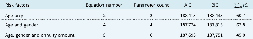
Table 2 shows the development of model fit from adding age, gender and annuity amount as mortality risk factors. As expected, the information criteria reduce as statistically significant risk factors are added. The sum of squared residuals does not have a similarly monotonic progression: moving from a model with age only to one with age and gender increases
 $\sum\nolimits_m r_m^2$
calculated against pension size. This is not an aberration: the same phenomenon is observed when calculating deviance residuals against duration (not shown).
$\sum\nolimits_m r_m^2$
calculated against pension size. This is not an aberration: the same phenomenon is observed when calculating deviance residuals against duration (not shown).
Table 2. Information Criteria (ICs) from Stepwise Inclusion of Age, Gender and Annuity Amount as Risk Factors
Mortality levels tend to vary monotonically by age. They also can be approximated as such for annuity amount, even if the fit for the very smallest annuities is not ideal. Thus, mortality by age and annuity amount can both be modelled using Hermite splines once each continuous variable is mapped onto the real interval
 $[0,1]$
. However, modelling mortality variation in calendar time is not monotonic, for which we need another kind of spline.
$[0,1]$
. However, modelling mortality variation in calendar time is not monotonic, for which we need another kind of spline.
6. Schoenberg Splines for Mortality Levels over Time
Mortality levels can fluctuate sharply over short periods of time, as shown in Figure 10, where seasonal variation is evident along with the COVID-19 shock in April 2020. Unlike mortality by age and annuity amount, patterns of mortality in time are not monotonic. We therefore require a method with sufficient local flexibility to reflect the rise and fall of mortality levels over time. For this, we use the splines of Schoenberg (Reference Schoenberg1964). Schoenberg’s splines are based on polynomials of degree bdeg spanning
 $(bdeg + 2)$
knot points. The knot points are unique values on the real line and in many applications they are uniformly spaced. However, uniform knot spacing is not mandatory (Kaishev et al., Reference Kaishev, Dimitrova, Haberman and Verrall2016) and section 8 will demonstrate an application of unequally spaced knots.
$(bdeg + 2)$
knot points. The knot points are unique values on the real line and in many applications they are uniformly spaced. However, uniform knot spacing is not mandatory (Kaishev et al., Reference Kaishev, Dimitrova, Haberman and Verrall2016) and section 8 will demonstrate an application of unequally spaced knots.

Figure 10. Mortality level in time for a mature US annuity portfolio using a semi-parametric estimator. The vertical dotted line indicates 1 April 2020. Source: Richards (Reference Richards2021b, Figure 3(c)).
Outside of a spline’s starting and end knots the spline takes the value 0, making it a purely local function. Figure 11 shows four Schoenberg splines of varying degrees, and more detail on such splines can be found in de Boor (Reference de Boor2001) and Eilers & Marx (Reference Eilers and Marx2021).

Figure 11. Schoenberg (Reference Schoenberg1964) splines with 1-year spacing between knot points (marked
 $ \bullet $
). (a)
$ \bullet $
). (a)
 $bdeg = 0$
, (b)
$bdeg = 0$
, (b)
 $bdeg = 1$
, (c)
$bdeg = 1$
, (c)
 $bdeg = 2$
and (d)
$bdeg = 2$
and (d)
 $bdeg = 3$
. In this specimen example, each spline is 0 before the knot at 2015 and 0 above the knot
$bdeg = 3$
. In this specimen example, each spline is 0 before the knot at 2015 and 0 above the knot
 $(bdeg + 1)$
knots to the right. The area under each spline is 1.
$(bdeg + 1)$
knots to the right. The area under each spline is 1.
Schoenberg splines are not new in mortality modelling: Eilers et al. (Reference Eilers, Currie and Durban2004) applied them to modelling mortality trends in grouped counts. This is done by forming a basis of cubic Schoenberg splines (B-splines) in calendar time, as shown in Figure 12.

Figure 12. A basis of nine equally-spaced cubic
 $B$
-splines spanning 1 January 2015 to 31 December 2020, indexed
$B$
-splines spanning 1 January 2015 to 31 December 2020, indexed
 $j = 0,1, \ldots ,8$
. Splines in solid black lie completely within the period, while splines in dashed grey are edge splines that only partly lie in the period being spanned. Knot points are marked
$j = 0,1, \ldots ,8$
. Splines in solid black lie completely within the period, while splines in dashed grey are edge splines that only partly lie in the period being spanned. Knot points are marked
 $ \bullet $
. Note that at any time-point
$ \bullet $
. Note that at any time-point
 $y \in [2015,2021]$
, there are always four non-zero splines that sum to 1. This is not true outside
$y \in [2015,2021]$
, there are always four non-zero splines that sum to 1. This is not true outside
 $[2015,2021]$
, meaning the method cannot extrapolate outside the calibration interval.
$[2015,2021]$
, meaning the method cannot extrapolate outside the calibration interval.
We define
 ${B_j}(y)$
as the
${B_j}(y)$
as the
 ${j^{{\rm{th}}}}$
basis spline evaluated at time y. Whereas formulae for Hermite h-splines are explicit, as in Figure 4, Schoenberg B-splines are typically defined by means of a recurrence relation; see de Boor (Reference de Boor2001, p. 90). We further define
${j^{{\rm{th}}}}$
basis spline evaluated at time y. Whereas formulae for Hermite h-splines are explicit, as in Figure 4, Schoenberg B-splines are typically defined by means of a recurrence relation; see de Boor (Reference de Boor2001, p. 90). We further define
 ${\mu _{x,y}}$
as the mortality hazard at exact age x and calendar time y. We can then use a B-spline basis as in Figure 12 to form an age-period model for
${\mu _{x,y}}$
as the mortality hazard at exact age x and calendar time y. We can then use a B-spline basis as in Figure 12 to form an age-period model for
 ${\mu _{x,y}}$
as per equation (7):
${\mu _{x,y}}$
as per equation (7):
 $$\log {\mu _{x,y}} = \log {\mu _x} + \sum\limits_{j \ge 1} {\kappa _{0,j}}{B_j}(y)$$
The parameter
 ${\kappa _{0,j}}$
corresponds to the
${\kappa _{0,j}}$
corresponds to the
 ${j^{{\rm{th}}}}$
B-spline, and summation is from
${j^{{\rm{th}}}}$
B-spline, and summation is from
 $j = 1$
as the spline
$j = 1$
as the spline
 $j = 0$
is absorbed into the baseline hazard. We use the zero subscript for the series
$j = 0$
is absorbed into the baseline hazard. We use the zero subscript for the series
 $\{ {\kappa _{0,j}}\} $
to distinguish it from the
$\{ {\kappa _{0,j}}\} $
to distinguish it from the
 $\kappa $
term used in a simpler approach to time-varying mortality in Richards (Reference Richards2020, section 7). To estimate the
$\kappa $
term used in a simpler approach to time-varying mortality in Richards (Reference Richards2020, section 7). To estimate the
 ${\kappa _{0,j}}$
along with any other parameters, we maximise the log-likelihood in equation (8):
${\kappa _{0,j}}$
along with any other parameters, we maximise the log-likelihood in equation (8):
 $$\matrix{ \ell \hfill \,{ = - \sum\limits_{i = 1}^n {H_{{x_i},{y_i}}}({t_i}) + \sum\limits_{i = 1}^n {d_i}\log {\mu _{{x_i} + {t_i},{y_i} + {t_i}}}} \hfill \cr \hskip-29pt{{H_{{x_i},{y_i}}}({t_i})} \,{ = \displaystyle\int_0^{{t_i}} {\mu _{{x_i} + s,{y_i} + s}}ds} \hfill \cr } $$
where life i enters observation at exact age
 ${x_i}$
at exact year
${x_i}$
at exact year
 ${y_i}$
, and is observed for exactly
${y_i}$
, and is observed for exactly
 ${t_i}$
years;
${t_i}$
years;
 ${H_{{x_i},{y_i}}}({t_i})$
is the integrated hazard that now depends on both age at entry and year of entry. Some sample estimates of
${H_{{x_i},{y_i}}}({t_i})$
is the integrated hazard that now depends on both age at entry and year of entry. Some sample estimates of
 ${\kappa _{0,j}}$
are given in Table 3, which are then applied to the
${\kappa _{0,j}}$
are given in Table 3, which are then applied to the
 ${B_j}$
in Figure 13 to show the local flexibility. Finally, the various
${B_j}$
in Figure 13 to show the local flexibility. Finally, the various
 ${\hat \kappa _{0,j}}{B_j}$
products are summed in Figure 14 to show how the estimated mortality level varies over time.
${\hat \kappa _{0,j}}{B_j}$
products are summed in Figure 14 to show how the estimated mortality level varies over time.
Table 3. Estimates of
 ${\kappa _{0,j}}$
for
${\kappa _{0,j}}$
for
 $j = 1,2, \ldots ,8$
for UK3 Portfolio, Using Data for the Age Range 55–105 years from 1 January 2015 to 31 December 2020.
$j = 1,2, \ldots ,8$
for UK3 Portfolio, Using Data for the Age Range 55–105 years from 1 January 2015 to 31 December 2020.
 ${\kappa _{0,0}} = 0$
by Construction because it is Absorbed into the Baseline Hazard
${\kappa _{0,0}} = 0$
by Construction because it is Absorbed into the Baseline Hazard


Figure 14. Schoenberg time spline function spanning 1 January 2015 to the end of 2020 using the basis splines in Figure 12 and the
 ${\hat \kappa _{0,j}}$
in Table 3. Panel (a) shows the unadjusted spline function, while panel (b) shows the function normalised at 0 at 2019.75, the last mid-point between a summer trough and winter peak before the COVID-19 pandemic. Note that summation in panel (b) is from
${\hat \kappa _{0,j}}$
in Table 3. Panel (a) shows the unadjusted spline function, while panel (b) shows the function normalised at 0 at 2019.75, the last mid-point between a summer trough and winter peak before the COVID-19 pandemic. Note that summation in panel (b) is from
 $j = 0$
because the coefficient of
$j = 0$
because the coefficient of
 ${B_0}$
is no longer 0.
${B_0}$
is no longer 0.
Note that absorbing
 ${\kappa _{0,0}}$
into the baseline as in equation (7) is just one way of specifying the necessary identifiability constraint, in this case
${\kappa _{0,0}}$
into the baseline as in equation (7) is just one way of specifying the necessary identifiability constraint, in this case
 ${\kappa _{0,0}} = 0$
. That a constraint is required comes from the identity in equation (9):
${\kappa _{0,0}} = 0$
. That a constraint is required comes from the identity in equation (9):
 $$\matrix{ \hskip-29pt{\log {\mu _{x,y}}} \,{ = {\alpha _0}{h_{00}}(u) + {\omega _0}{h_{01}}(u) + \sum\limits_{j \ge 0} ({\kappa _{0,j}} - c){B_j}(y)} \hfill \cr {} \hfill \cr\,{ = {\alpha _0}{h_{00}}(u) + {\omega _0}{h_{01}}(u) - c + \sum\limits_{j \ge 0} {\kappa _{0,j}}{B_j}(y),\quad {\rm{a}}s\;\sum\limits_{j \ge 0} c{B_j}(y) = c,\forall c \in \mathbb R} \hfill \cr {} \hfill \cr\,{ = ({\alpha _0} - c){h_{00}}(u) + ({\omega _0} - c){h_{01}}(u) + \sum\limits_{j \ge 0} {\kappa _{0,j}}{B_j}(y),\quad {\rm{a}}s\;{h_{00}}(u) + {h_{01}}(u) = 1} \hfill \cr } $$
Without an identifiability constraint, there is an infinite choice of real-valued c that can be deducted from each
 ${\kappa _{0,j}}$
and added to
${\kappa _{0,j}}$
and added to
 ${\alpha _0}$
and
${\alpha _0}$
and
 ${\omega _0}$
in equations (1) or (2) and still yield the same fit. As a consequence, the vertical scale in Figure 14(a) is somewhat arbitrary and depends in large part on the mortality experience covered by the right-hand part of spline
${\omega _0}$
in equations (1) or (2) and still yield the same fit. As a consequence, the vertical scale in Figure 14(a) is somewhat arbitrary and depends in large part on the mortality experience covered by the right-hand part of spline
 ${B_0}$
(see e.g. the spline
${B_0}$
(see e.g. the spline
 $j = 0$
in Figure 12 relative to the period from 1 January 2015).
$j = 0$
in Figure 12 relative to the period from 1 January 2015).
We can use equation (9) to normalise the Schoenberg spline function to take the value 0 at a particular point in calendar time. This is useful if we regard that point in time as having a meaning and we want to compare subsequent mortality levels (as is done in Figure 17, for example). For example, 1 October 2019 (2019.75 decimalised) represents the last mid-point between a summer trough and a winter peak before the COVID-19 pandemic, and so might be regarded as the most recent suitable time point unaffected by seasonal swings, pandemic shocks and unreported deaths. If we define
 ${c_{2019.75}} = \sum\nolimits_{j \ge 1} {\hat \kappa _{0,j}}{B_j}(2019.75)$
, we can then deduct this value from each
${c_{2019.75}} = \sum\nolimits_{j \ge 1} {\hat \kappa _{0,j}}{B_j}(2019.75)$
, we can then deduct this value from each
 ${\hat \kappa _{0,j}}$
and normalise the Schoenberg spline function without distorting the model fit as long as we also add
${\hat \kappa _{0,j}}$
and normalise the Schoenberg spline function without distorting the model fit as long as we also add
 ${c_{2019.75}}$
to the estimates
${c_{2019.75}}$
to the estimates
 ${\hat \alpha _0}$
and
${\hat \alpha _0}$
and
 ${\hat \omega _0}$
(
${\hat \omega _0}$
(
 ${c_{2019.75}}$
of course needs to be recalculated whenever the knot points in the spline basis change). Figure 14(b) shows the resulting normalised Schoenberg spline.
${c_{2019.75}}$
of course needs to be recalculated whenever the knot points in the spline basis change). Figure 14(b) shows the resulting normalised Schoenberg spline.
7. Modelling Seasonal Variation and COVID-19 Shocks
Mortality has long been known to have a major seasonal component; Rau (Reference Rau2007, Chapter 2) gives a comprehensive introduction, covering both historical and modern aspects. Seasonal variation is also pronounced in pensioner mortality, as demonstrated by Richards et al. (Reference Richards, Ramonat, Vesper and Kleinow2020) with a recurring annual cosine term. Such an approach estimates an average seasonal effect within each year, with peak mortality in winter and low mortality in summer. However, this approach cannot account for years with heavier-than-average winter mortality, nor will it account for slight shifts in the timing of the winter peak.
We can address these issues by increasing the number of knots per year. This increases the number of splines needed to span 2015–2020, with the resulting mortality level shown in Figure 15 for two, four and ten knots per year.

Figure 15. Addition to log(hazard) using equally spaced knots, normalised at 0 for 1 October 2019. (a) Two2 knots per year, (b) four knots per year and (c) ten knots per year.
Figure 15(a) shows that using two knots per year picks up the seasonal variation with the winter peaks around January of each year 2015–2019. The exception is 2020, where the expected winter peak in January has merged with the COVID-19 mortality spike of April and May 2020, resulting in an aggregate peak shifted more towards the time of the first COVID-19 shock. Another feature of Figure 15(a) is the deep trough leading up to the end of 2020; this could be either a real feature of the data, say due to the COVID-19 mortality being partly due to brought-forward deaths, or else an artefact from the B-spline basis having insufficient flexibility to cope with the short-term intensity of the two COVID-19 shocks in Figure 3. To resolve this, we can increase the knot density further, as in Figure 15(b) and (c), but we face a difficult balancing act – increasing the knot density allows the nature of the COVID-19 spike to come through, but at the expense of weakening the signal at other times.
Table 4 summarises the model fits using various equally spaced knot densities. According to the AIC, the model with ten knot points per year is the best fit, which is rather contradicted by the fluctuations in Figure 15(c). In contrast, the BIC indicates that two knot points per year is the best fit. The conflicting messages are likely due to the large number of parameters not being penalised as heavily in the AIC. In mainstream statistical work, a small-sample correction to the AIC is often used because of this (Macdonald et al., Reference Macdonald, Richards and Currie2018, p. 98). However, in actuarial work, the sample size is typically not a problem due to there being tens of thousands of data points (
 $n = 116,056$
for the UK3 portfolio here). Rather, the issue is a large number of parameters for a given risk factor – with four or more knot points per year, many of the
$n = 116,056$
for the UK3 portfolio here). Rather, the issue is a large number of parameters for a given risk factor – with four or more knot points per year, many of the
 ${\kappa _{0,j}}$
parameters prior to the mortality shock are not explaining enough variation to justify their inclusion. Ye (Reference Ye1998, p. 120) notes that “flexibility often leads to substantial overfitting.” A possible explanation for the failure of the AIC is given by Owen (Reference Owen1991, pp. 102–103), albeit in the context of a different model — where a statistically significant parameter is being estimated, the estimation costs one degree of freedom; however, if the parameter is statistically insignificant, the estimation costs more than one degree of freedom. Thus, where unnecessary spline parameters are introduced, the standard definition of the AIC may fail to properly penalise this. We will consider this drawback of the AIC again in sections 11 and 12.
${\kappa _{0,j}}$
parameters prior to the mortality shock are not explaining enough variation to justify their inclusion. Ye (Reference Ye1998, p. 120) notes that “flexibility often leads to substantial overfitting.” A possible explanation for the failure of the AIC is given by Owen (Reference Owen1991, pp. 102–103), albeit in the context of a different model — where a statistically significant parameter is being estimated, the estimation costs one degree of freedom; however, if the parameter is statistically insignificant, the estimation costs more than one degree of freedom. Thus, where unnecessary spline parameters are introduced, the standard definition of the AIC may fail to properly penalise this. We will consider this drawback of the AIC again in sections 11 and 12.
Table 4. Information Criteria (ICs) for Various Knot Densities with Equal Spacing. UK3 Portfolio for 1 January 2015 to the End of 2020. ICs and Parameter Counts can be Compared with Table 2 as the Underlying Data are Identical. The Optimal AIC and BIC Values are Marked in Bold

8. Increasing the Knot Density Around Shock Times
Figure 15(c) shows that increasing the density of the knot points allows the COVID-19 mortality shock to be clearly identified in terms of height and timing. However, the development from Figure 15(a) to (c) also suggests the introduction of random variation for the non-COVID period. It is undesirable to add knot points where flexibility is not required, so we address this by providing extra knots only where they are needed. One approach is to use half-yearly spaced knots for all years, but to add extra knots around the time of the first COVID-19 spike in April and May 2020, as shown in Figure 16. We justify this from our a priori knowledge of the population COVID-19 mortality in Figure 3.

Figure 16. Part of a basis of nineteen variably spaced cubic B-splines spanning 1 January 2015 to the end of 2020, indexed
 $j = 0,1, \ldots ,18$
(only splines
$j = 0,1, \ldots ,18$
(only splines
 $j = 10, \ldots ,18$
are shown). Splines in solid black lie completely within the period, while splines in dashed grey are edge splines that only partly lie in the period being spanned. Knot points are marked
$j = 10, \ldots ,18$
are shown). Splines in solid black lie completely within the period, while splines in dashed grey are edge splines that only partly lie in the period being spanned. Knot points are marked
 $ \bullet $
.
$ \bullet $
.
Figure 17 shows the resulting mortality levels in time, with the expected seasonal fluctuations and the first COVID-19 spike around April 2020. The mixed approach with two knots per year for pre-COVID years and additional knots for the pandemic shock works well in capturing the salient features in time. Figure 17(b) further shows the usefulness of normalising the Schoenberg splines at 0 at a point in time – when converted to the hazard scale the multiplier is 1 at the reference point (2019.75 in this case) and we can see that the peak of the COVID-19 spike is nearly double the reference level of mortality. Following the shock in April 2020, there is also an unusually deep summer trough in 2020, which could be a result of “harvesting” due to brought-forward deaths of the frail. Figure 17(b) also shows that the pre-pandemic seasonal trough-to-peak variation varies between around 15–30%, which is consistent with the results in Richards et al. (Reference Richards, Ramonat, Vesper and Kleinow2020, Table 2) for a variety of international annuity and pension portfolios.

Figure 17. Mortality level modelled using the spline basis depicted in Figure 16. Panel (a) shows the addition to log(mortality), while panel (b) shows the multiplier of the mortality hazard.
The BIC for the model behind Figure 17 is 187,489, which is considerably lower than any of the BICs in Table 4. This suggests that the basis of variably spaced knots in Figure 16 has provided flexibility only where it is needed. The time signal is relatively strong: dropping the factors gender and annuity amount from the model leaves Figure 17 largely unchanged, which justifies the age plus period nature of equation (7). However, the BIC for the model behind Figure 17 does not take into account the fact that the knots were selected with reference to data and judgement (specifically, a comparison of the plots in Figure 15 and the distribution of COVID-19 deaths in Figure 3). The question of defining and using information criteria is discussed further in section 12.
There are at least two other alternative approaches that would be possible. The first is the optimisation of the number and position of knots by an algorithm targeting a measure of fit; Kaishev et al. (Reference Kaishev, Dimitrova, Haberman and Verrall2016) propose a knot-addition algorithm and also give a comprehensive overview of related knot optimisation research. The second approach is to deliberately use too many knots and use a tuning parameter to minimise the variability exhibited in Figure 15(c); Eilers & Marx (Reference Eilers and Marx1996) give details. However, both of these methods have huge computational cost when applied to actuarial data sets, where the observations often number hundreds of thousands. For example, the UK3 data set in this paper has
 $n = 116,056$
records and the model behind Figure 17 has 19 Schoenberg splines, giving a knot-to-data ratio of around 1:6,000. In contrast, the data set from Kimber et al. (Reference Kimber, Kreyssig, Zhang, Jeschke, Valenti, Yokaichiya, Colombier, Yan, Hansen, Chatterji, McQueeney, Canfield, Goldman and Argyriou2009) reworked by Kaishev et al. (Reference Kaishev, Dimitrova, Haberman and Verrall2016) involves just 1,151 observations and has 227 knots, giving a knot-to-data ratio of 1:5. The model behind Figure 17 took 1.5 hours to fit using parallel processing over 63 threads (Butenhof, Reference Butenhof1997), so adding lots more splines – as per Eilers & Marx (Reference Eilers and Marx1996) – would result in much longer run times. Similarly, the repeated refitting with new knots – as per Kaishev et al. (Reference Kaishev, Dimitrova, Haberman and Verrall2016) – would also be time-consuming when applied to actuarial data sets.
$n = 116,056$
records and the model behind Figure 17 has 19 Schoenberg splines, giving a knot-to-data ratio of around 1:6,000. In contrast, the data set from Kimber et al. (Reference Kimber, Kreyssig, Zhang, Jeschke, Valenti, Yokaichiya, Colombier, Yan, Hansen, Chatterji, McQueeney, Canfield, Goldman and Argyriou2009) reworked by Kaishev et al. (Reference Kaishev, Dimitrova, Haberman and Verrall2016) involves just 1,151 observations and has 227 knots, giving a knot-to-data ratio of 1:5. The model behind Figure 17 took 1.5 hours to fit using parallel processing over 63 threads (Butenhof, Reference Butenhof1997), so adding lots more splines – as per Eilers & Marx (Reference Eilers and Marx1996) – would result in much longer run times. Similarly, the repeated refitting with new knots – as per Kaishev et al. (Reference Kaishev, Dimitrova, Haberman and Verrall2016) – would also be time-consuming when applied to actuarial data sets.
9. Estimating Portfolio-Specific Improvements
An advantage of equation (7) is that it can be used to estimate the portfolio-specific mortality improvement (PSMI). This can be estimated by selecting either two winter peaks or two summer troughs at time points
 ${y_1} \lt {y_2}$
and using equation (10):
${y_1} \lt {y_2}$
and using equation (10):
 $$PSMI = \left[ {1 - \exp \left( {{{\sum\limits_{j \ge 1} {{\kappa _{0,j}}} ({B_j}({y_2}) - {B_j}({y_1}))} \over {{y_2} - {y_1}}}} \right)} \right] \times 100\% $$
Our preference is to use summer troughs due to the tendency for sharp peaks in winter and relatively flat troughs in summer (Marx et al., Reference Marx, Eilers, Gampe and Rau2010), meaning that winter peaks can be more extreme and variable. From Figure 17(a), the period 2015.5–2019.5 seems to be the most suitable period for estimating the portfolio-specific improvement rate, as the trough in the summer of 2020 may be unusually deep due to brought-forward deaths. With
 ${y_1} = 2015.5$
and
${y_1} = 2015.5$
and
 ${y_2} = 2019.5$
, equation (10) gives
${y_2} = 2019.5$
, equation (10) gives
 $PSMI = \left[ {1 - \exp \left( {{{ - 1.00971 - ( - 0.96219)} \over {2019.5 - 2015.5}}} \right)} \right] \times 100\% = 1.18\% $
p.a. This is an age-independent mortality improvement rate, as equation (7) is an “age plus period effect” model.
$PSMI = \left[ {1 - \exp \left( {{{ - 1.00971 - ( - 0.96219)} \over {2019.5 - 2015.5}}} \right)} \right] \times 100\% = 1.18\% $
p.a. This is an age-independent mortality improvement rate, as equation (7) is an “age plus period effect” model.
Table 5 shows the improvement rates for various combinations of summer troughs in Figure 17. Of interest are the strong improvement rates ending in summer 2020 (2020.5), indicating the depth of the mortality dip following the first COVID-19 shock in April 2020. This phenomenon is unrelated to late-reported deaths, which is the subject of section 10. However, it is an open question as to what value such volatile improvement rates have when summer troughs can be almost as variable as winter peaks.
Table 5. Annualised Improvement Rates (
 $PSMI$
) between Summer Troughs in Figure 17
$PSMI$
) between Summer Troughs in Figure 17

10. OBNR Deaths
Although the UK3 portfolio data include experience to the end of June 2021, we have so far only used the experience to the end of 2020 to minimise the impact of delays in death reporting. Richards (Reference Richards2021b, Figure 7) examined the reporting delays for the same portfolio and found minimal impact on mortality experience a quarter of a year or more before the extract date, so discarding the most recent half-year of experience should be more than enough to eliminate OBNR effects. However, discarding experience data is undesirable if it can be avoided, and Richards (Reference Richards2021b) proposed a parametric model for late-reported deaths as a means of using all available data without distorting the final results.
However, the reduction in reported mortality leading up to the extract date is just another pattern in time, which means that the Schoenberg spline function in equation (7) is also an alternative means of allowing for late-reported deaths. We can therefore extend the spline basis and include all available experience data, including the period most affected by late-reported deaths. The result is presented in Figure 18, which shows not only a multiplicative factor falling to 0 at the extract date at the end of June 2021, but also the second COVID-19 spike of January 2021. Figure 3 suggests that the second COVID-19 spike should be around the same height as the first, and so it is possible that the lower spike in January 2021 in Figure 18 is due to some OBNR deaths. We could in theory use the forecasting method of Richards (Reference Richards2021b, section 7) to adjust for this, but a parametric OBNR model will not easily fit due to the high correlation with the last spline parameter. However, it is more likely that the first peak in Figure 3 is due to COVID-19 deaths not being recorded as such.

Figure 18. Hazard multiplier using the spline basis depicted in Figure 16 and extended with more knots to cover Q1 2021. The identifiability constraint is that at 1 October 2019 (2019.75 decimalised) the multiplier is normalised at 1.
11. Schoenberg Splines for Mortality by Age
The demonstrable effectiveness of Schoenberg splines when applied to time-varying mortality raises the question whether we should not also use them for mortality by age. This is not a new idea – McCutcheon (Reference McCutcheon1979) used cubic splines by age when graduating mortality tables, for example. However, the approach of McCutcheon (Reference McCutcheon1979) was designed for stratified grouped data, and not the inclusion of additional covariates per life.
For application to a survival model for individual lives, we therefore use equation (11):
 $$\log {\mu _x} = {\alpha _0} + \sum\limits_{k \ge 1} {\alpha _{0,k}}{B_k}(x)$$
where
 ${\alpha _0}$
is the baseline,
${\alpha _0}$
is the baseline,
 ${B_k}(x)$
is the
${B_k}(x)$
is the
 ${k^{{\rm{th}}}}$
B-spline evaluated at exact age x and
${k^{{\rm{th}}}}$
B-spline evaluated at exact age x and
 ${\alpha _{0,k}}$
is the corresponding spline parameter. As before, summation is from
${\alpha _{0,k}}$
is the corresponding spline parameter. As before, summation is from
 $k = 1$
because the spline
$k = 1$
because the spline
 $k = 0$
is absorbed into the baseline.
$k = 0$
is absorbed into the baseline.
Figure 19 shows the AIC and BIC for various knot spacings for
 ${B_k}(x)$
. As with Table 4, the two information criteria give conflicting guidance on which model to pick: the AIC indicates that the best knot spacing in age is 4 years, while the BIC suggests that the optimum knot spacing is 25 years or more.
${B_k}(x)$
. As with Table 4, the two information criteria give conflicting guidance on which model to pick: the AIC indicates that the best knot spacing in age is 4 years, while the BIC suggests that the optimum knot spacing is 25 years or more.

Figure 19. (a) AIC, (b) BIC and (c) number of spline parameters for UK3 mortality rates using model in equation (11) and various equidistant knot spacings. Ages covered are 55–105 years from 1 January 2015 to 31 December 2020.
One reason to reject the AIC-recommended 4-year knot spacing is shown in Figure 20. The model is over-fitted at both the youngest and oldest ages: we have no reason to believe that mortality rates decline at the oldest ages, and the single death at the age of 55 years is not grounds enough for the fitted shape. This is then an advantage of the Hermite spline approach of equation (1) — it has fewer parameters and less flexibility, thus only permitting slow and stable changes with age. Alternatively, a basis of widely spaced Schoenberg splines will behave similarly. However, we note that the Hermite spline approach of equation (6) is better suited to the modelling of post-retirement mortality due to automatic convergence of differentials with increasing age (Richards, Reference Richards2020, section 3).

Figure 20. Crude mortality hazard at each age,
 $x$
, and fitted curve using equation (11) and a 4-year knot spacing, showing over-fitting. Source: own calculations using UK3 data.
$x$
, and fitted curve using equation (11) and a 4-year knot spacing, showing over-fitting. Source: own calculations using UK3 data.
In Figure 20, we see that excessive flexibility from closely spaced Schoenberg splines in age is undesirable – the fit might be superficially better quantitatively in terms of the AIC, but is poorer qualitatively when one takes into account data quality and reasonable prior expectations. However, there will be occasions when the greater flexibility of closely spaced Schoenberg splines is useful, such as where younger ages are included. Figure 21 shows an example of a non-monotonic pattern with age, for which Hermite splines will be unsuitable and for which greater flexibility is required.

Figure 21. Graduated mortality rates for Australian males, showing accident hump around the age of 20 years. Source: Heligman & Pollard (Reference Heligman and Pollard1980, Figure 12).
12. Information Criteria and Actuarial Judgement
In this paper, we have seen two instances where the AIC led to a qualitatively poorer choice of knot spacing for Schoenberg splines for mortality: first for a time-varying function in Figure 15(a) and again for an age-varying function in Figure 20. In both cases, the AIC led to an excessive number of parameters and over-fitting. Using the small-sample correction for the AIC (Hurvich & Tsai, Reference Hurvich and Tsai1989) would not have led to a different outcome due to the large number of observations (Macdonald et al., Reference Macdonald, Richards and Currie2018, Table 6.1).
The definitions of the AIC and BIC used in this paper are the usual ones given in section 4 and used in Figures 19(a) and (b). However, it is worth noting that more rigorous definitions are given in equation (12), where
 $\ell $
is the log-likelihood from equation (3), n is the number of lives and df is the number of degrees of freedom used. In equation (12), it is common to use
$\ell $
is the log-likelihood from equation (3), n is the number of lives and df is the number of degrees of freedom used. In equation (12), it is common to use
 $df = p$
, where p is the number of parameters; for a simple linear regression model, the two are synonymous. However, Owen (Reference Owen1991, p. 103) noted that it is possible for a non-linear model to have
$df = p$
, where p is the number of parameters; for a simple linear regression model, the two are synonymous. However, Owen (Reference Owen1991, p. 103) noted that it is possible for a non-linear model to have
 $df \gt p$
, while Ye (Reference Ye1998, p. 122) notes that even a linear smoother can have fewer degrees of freedom than there are parameters (
$df \gt p$
, while Ye (Reference Ye1998, p. 122) notes that even a linear smoother can have fewer degrees of freedom than there are parameters (
 $df \lt p$
). In the field of mortality modelling, Macdonald et al. (Reference Macdonald, Richards and Currie2018, section 11.6) give an example of a penalised Generalized Linear Model where the effective degrees of freedom are
$df \lt p$
). In the field of mortality modelling, Macdonald et al. (Reference Macdonald, Richards and Currie2018, section 11.6) give an example of a penalised Generalized Linear Model where the effective degrees of freedom are
 $df = 9.0$
with
$df = 9.0$
with
 $p = 20$
regression coefficients. Assuming that
$p = 20$
regression coefficients. Assuming that
 $df = p$
is a simplifying assumption only, and actuaries should not automatically pick a model solely because of its low information criterion.
$df = p$
is a simplifying assumption only, and actuaries should not automatically pick a model solely because of its low information criterion.
 $$\matrix{ {AIC} \;{ = - 2\ell + 2df} \hfill \cr {BIC} \;\hfill { = - 2\ell + df\log n} \hfill \cr } $$
This problem of the AIC leading to over-fitting may be restricted to relatively large numbers of parameters for a given risk factor. However, relying only on the BIC as an alternative is not a complete solution either for actuarial work. For example, there is a distinction between risk factors that are statistically significant and those that are financially significant; Richards (Reference Richards2020, section 9) gives several contrasting examples. In Figure 6, the large negative residuals for the lowest and highest size bands are of equal significance statistically, yet actuaries will tolerate a poorer fit for smaller amounts if it means better explaining the mortality of those with the largest annuity amounts. While the BIC might be the better information criterion, it cannot be the sole arbiter of model selection for actuarial purposes.
Leaving aside the complexities of model selection, there is also the practical question of how to turn a complex, multi-factor model into a mortality basis. In the bulk annuity and longevity swap markets, specialist valuation software is required to handle the complexities of UK pensioner benefits. However, such valuation systems are seldom capable of handling multi-factor models, and usually a table of mortality rates by age and gender is all that can be accommodated. A useful conversion tool is the equivalent reserve method of Willets (Reference Willets1999), which expresses one mortality basis in terms of another via the medium of the liabilities in question. For the sake of example, assume that we want to express current mortality levels in terms of the equivalent percentages of some third-party table. We are interested in the mortality rates appplying at a point in time, so we ignore future mortality improvements, as these are usually a separate basis item. The approach of Willets (Reference Willets1999) is to solve equation (13) for males and females separately:
 $$\sum\limits_i {a_i}\displaystyle\int_0^\infty {v^t}_tp_x^{\rm model}dt = \sum\limits_i {a_i}\displaystyle\int_0^\infty {v^t}_tp_x^{\rm table}dt$$
where
 ${a_i}$
is the annuity amount for life i,
${a_i}$
is the annuity amount for life i,
 ${v^t}$
is the net discount function to apply to a payment in t years,
${v^t}$
is the net discount function to apply to a payment in t years,
 $_tp_x^{\rm model}$
is the survival probability according to the model and
$_tp_x^{\rm model}$
is the survival probability according to the model and
 $_tp_x^{\rm table}$
is the survival probability according to the published table. We do not need to worry about the distorting effect of ignoring mortality improvements, as long as they are ignored on both sides of equation (13). In general,
$_tp_x^{\rm table}$
is the survival probability according to the published table. We do not need to worry about the distorting effect of ignoring mortality improvements, as long as they are ignored on both sides of equation (13). In general,
 $_t{p_x} = \exp \left( { - \int_0^t {\mu _{x + s}}ds} \right)$
, and we use the definition of the mortality hazard in equation (14):
$_t{p_x} = \exp \left( { - \int_0^t {\mu _{x + s}}ds} \right)$
, and we use the definition of the mortality hazard in equation (14):
 $$\mu _x^{\rm table} = f\mu _x^{\rm S2PA}$$
where
 $\mu _x^{\rm S2PA}$
is the mortality hazard according to the table S2PA (CMI Ltd, 2014), and f is the percentage of that table to be solved for in equation (13). Figure 22 shows the results using the modelled mortality levels applying at various points in time over 2019–2020, assuming – somewhat unrealistically – that those mortality levels continue indefinitely, that is, for the calculation using mortality levels at outset time y the integrated hazard is
$\mu _x^{\rm S2PA}$
is the mortality hazard according to the table S2PA (CMI Ltd, 2014), and f is the percentage of that table to be solved for in equation (13). Figure 22 shows the results using the modelled mortality levels applying at various points in time over 2019–2020, assuming – somewhat unrealistically – that those mortality levels continue indefinitely, that is, for the calculation using mortality levels at outset time y the integrated hazard is
 ${H_x}(t) = \displaystyle\int_0^\infty {\mu _{x + s,y}}$
.
${H_x}(t) = \displaystyle\int_0^\infty {\mu _{x + s,y}}$
.

Figure 22. Percentages of S2PA implied by mortality levels over 2019–2020. Liabilities for UK3 at 1 January 2021 equated as per equation (13) using a net discount rate of 0% p.a. (
 ${v^t} = 1,\forall t$
).
${v^t} = 1,\forall t$
).
Figure 22 shows the extent of the challenge for actuaries in setting the best-estimate mortality basis for pricing bulk annuities or longevity swaps. Under normal circumstances, one might pick the most recent mid-point between a summer trough and a winter peak; 75–76% for males and 70–71% for females in October 2020, say. As it happens, mortality at this point in time was largely unaffected by COVID-19 (see Figure 3), but the equivalent percentages for April and May 2020 show the discontinuities possible due to pandemic mortality. The equivalent percentages for January 2020 show an emerging second discontinuity due to the second COVID-19 shock as shown in Figures 3 and 18.
Of course, no actuary would use equivalent percentages like those for April and May 2020 in Figure 22. However, the importance of allowing for the mortality shock can be seen from imagining what the results would be like without it: without the flexibility of the Schoenberg splines in time, the shock points would be moved down and all the other percentages in Figure 22 would be shifted up; any resulting basis would thus be imprudent for pricing a bulk annuity or longevity swap. The value of the methodology lies in accommodating the mortality spikes so that they cannot drive bias at other points in time.
13. Conclusions
For continuous variables where mortality varies either monotonically or with simple shape variation, a basis of Hermite splines usually provides all the flexibility that is needed. Examples include mortality by age and annuity amount. For actuarial purposes, quality of fit for the smallest annuity amounts is less important than the fit for the largest amounts.
In contrast, continuous variables where mortality fluctuates a lot, or where fluctuations are sharp and extreme, are better handled by a basis of local splines. Using cubic Schoenberg splines (B-splines), we can model mortality levels across time for annuity portfolios and pension funds. With two knot points per year, we can identify seasonal variation in mortality, and we can estimate portfolio-specific mortality improvements from the change in mortality levels between summer troughs. Where the number of observations is large, we find that the BIC is materially better for selecting the number of knot points than the AIC.
To handle mortality shocks like COVID-19, we add additional knot points from our a priori knowledge of the timing of mortality spikes in the population. This mixed approach of regular half-yearly knots and hand-placed additional knots allows the salient mortality features to be identified, that is, both seasonal variation and mortality shocks. A benchmark time point can be selected to use in setting a basis, safe in the knowledge that the model’s other parameters are not unduly biased due to the presence of shocks because their effects are explicitly modelled.
The flexibility of the local Schoenberg splines further allows the modelling of the impact of late-reported deaths. This removes the need to discard the most recent experience data and thus permits the use of all available data for analysis and basis setting.
Acknowledgements
The author thanks Anil Gandhi and Caroline Roberts for their support in providing data. The author also thanks Gavin Ritchie, Torsten Kleinow, Stefan Ramonat, Prof. Angus Macdonald and two anonymous reviewers for helpful comments on earlier drafts of this paper. Any errors or omissions remain the responsibility of the author. Calculations were performed using the Longevitas survival modelling system. Graphs were produced in tikz, pgfplots and R.
Disclaimer:
The views expressed in this publication are those of invited contributors and not necessarily those of the Institute and Faculty of Actuaries. The Institute and Faculty of Actuaries do not endorse any of the views stated, nor any claims or representations made in this publication and accept no responsibility or liability to any person for loss or damage suffered as a consequence of their placing reliance upon any view, claim or representation made in this publication. The information and expressions of opinion contained in this publication are not intended to be a comprehensive study, nor to provide actuarial advice or advice of any nature and should not be treated as a substitute for specific advice concerning individual situations. On no account may any part of this publication be reproduced without the written permission of the Institute and Faculty of Actuaries.
Appendices
A. Implementation
A general approach to fitting left-truncated survival models is presented in Richards (Reference Richards2020, Appendix B). The starting point is the log-likelihood,
 $\ell $
, defined in equation (8). The contribution of a single life i to the log-likelihood is given in equation (15):
$\ell $
, defined in equation (8). The contribution of a single life i to the log-likelihood is given in equation (15):
 $${\ell _i} = - \left[ {\displaystyle\int_0^{{t_i}} {\mu _{{x_i} + s,{y_i} + s}}ds} \right] + {d_i}\log {\mu _{{x_i} + {t_i},{y_i} + {t_i}}}$$
To maximise the log-likelihood function, we require the gradient with respect to each parameter, and to estimate standard errors we require the second pure and cross-derivatives for all parameters. General formulae are given in Richards et al. (Reference Richards, Ramonat, Vesper and Kleinow2020, Appendix A).
The nature of the mortality hazards in equations (1), (2), (4), (7) and (11) means that closed-form expressions for the integrated hazard in equation (15) do not exist. For the results in this paper, we have used the Romberg method of numerical integration, but Clenshaw–Curtis integration is also an option. Richards et al. (Reference Richards, Ramonat, Vesper and Kleinow2020, Appendix A) discuss some practical tests for ensuring that numerical integration has taken place sufficiently accurately. Due to the computationally intensive nature of the calculations, we process work in parallel across 63 threads (Butenhof, Reference Butenhof1997). For the summation of lots of potentially small contributions like equation (15), we use the floating point error correction algorithm of Kahan (Reference Kahan1965).
Where a material OBNR effect exists, as in Figure 18, the value of
 ${\hat \kappa _j}$
can be large and negative for the rightmost spline; in the model behind Figure 18, for example,
${\hat \kappa _j}$
can be large and negative for the rightmost spline; in the model behind Figure 18, for example,
 ${\hat \kappa _j} \in ( - 5,4),\forall j \in \{ 1, \ldots ,22\} $
, but
${\hat \kappa _j} \in ( - 5,4),\forall j \in \{ 1, \ldots ,22\} $
, but
 ${\hat \kappa _{23}} = - 66.5$
. This can lead to a large number of iterations where the algorithm for optimising the log-likelihood places a limit on the size of the change in parameter estimates; examples include the parscale control parameter in R Core Team (2017, optim function) and the STPMX variable in Press et al. (Reference Press, Teukolsky, Vetterling and Flannery2005, dfpmin function). To reduce the number of iterations, the limit on the step size between successive parameters can be increased, or an adaptive step size used when the number of iterations proves large. In our implementation, we double the maximum step size every 50 iterations – this has little impact on most models with parameters in the range
${\hat \kappa _{23}} = - 66.5$
. This can lead to a large number of iterations where the algorithm for optimising the log-likelihood places a limit on the size of the change in parameter estimates; examples include the parscale control parameter in R Core Team (2017, optim function) and the STPMX variable in Press et al. (Reference Press, Teukolsky, Vetterling and Flannery2005, dfpmin function). To reduce the number of iterations, the limit on the step size between successive parameters can be increased, or an adaptive step size used when the number of iterations proves large. In our implementation, we double the maximum step size every 50 iterations – this has little impact on most models with parameters in the range
 $( - 20, + 20)$
but adapts to cope with models with extreme parameter values caused by OBNR.
$( - 20, + 20)$
but adapts to cope with models with extreme parameter values caused by OBNR.
B. Model Parameters
There are two groups of model parameters to be set for the mortality models in this paper: (i) configuration settings, whose values are decided in advance by the analyst and (ii) parameters whose values are estimated from the data.
B.1. Model Settings Decided by the Analyst
Table B.1 lists the configuration settings that need to be decided in advance by the analyst, that is, they are not estimated from the data. Where appropriate, the values used in the main body of the paper are given.
Table B.1. Configuration Parameters

Other analyst decisions include the identifiability constraint on the
 $\{ {\kappa _{0,j}}\} $
parameters (we use
$\{ {\kappa _{0,j}}\} $
parameters (we use
 ${\kappa _{0,0}} = 0$
) and the knot spacing.
${\kappa _{0,0}} = 0$
) and the knot spacing.


 Open access