


1. Introduction
Corporate income tax (hereafter, CIT) has detrimental effects on investment by firms. Modern prevailing opinions advocate that CIT should be cut to promote economic growth. Governments in developed countries have lowered the CIT rate in recent years: The average rate of CIT in OECD countries decreased from 32.5% to 24.2% between 2000 and 2017.Footnote 1 However, because CIT is an important tax basis for public finance, cutting the CIT rate reduces public investment in infrastructure (productive public services) and may lower the rate of economic growth (e.g., Barro (Reference Barro1990)).Footnote 2 Therefore, setting CIT rates involves a trade-off between private investment and the provision of productive public services for economic growth, and it is an important policy issue.
In addition, tax evasion by firms is a serious problem of CIT. There is large-scale tax evasion in real economies. For example, in the USA, from 2008 to 2010, the Internal Revenue Service (2016) reported an annual average of about 44 billion dollars in the estimated tax gaps of CIT (the amount of true tax liability that is not paid voluntarily and timely).Footnote 3 Nonetheless, the actual audit coverage of taxed corporations is very limited, primarily because of fiscal tightness; only 1.0% of taxed returns were examined in the USA in 2016, and only 3.1% of all taxed corporations were audited in Japan in 2015.Footnote 4
One of the most general ways of tax evasion is to under-declare income (e.g., Allingham and Sandmo (Reference Allingham and Sandmo1972)). To under-declare corporate income, firms may understate their productivity and overstate their costs. There is institutional cause for such tax evasion behavior at the microeconomic level. The CIT systems in many countries have reduction and exemption measures; deficits of corporations can be carried forward and CITs of corporations with small income are reduced or exempted. Such systems give corporations a loophole to under-declare their profit intentionally by overstating cost. These are neither unusual nor insignificant at the macroeconomic level. For example, the National Tax Agency (2016) reports that, on average, more than two-thirds of the ordinary corporations in Japan were loss-making corporations between 2011 and 2015. The reported losses amounted to 11.3 billion yen in 2015 and occupied a quarter of the reported total income in the corporate sector.
With these problems of CIT as motivation, this study investigates an optimal CIT policy in a growing economy with tax evasion by firms. The evaded tax payments are utilized for private investment, while a part of the tax revenue is lost. This affects the trade-off between private investment and the provision of productive public services. We are particularly interested in how CIT evasion by firms changes the optimal rate of CIT.
To tackle this problem, we construct a variety-expansion model of growth in which private firms invest to earn monopolistic profits and their investments sustain economic growth.Footnote 5 A single final good is produced by using intermediate goods. Each intermediate good is produced by a monopolistically competitive firm. Each intermediate good firm invests to enter into business and pursues monopolistic profits. CIT discourages private investment because the monopolistic profits are subject to CIT. Meanwhile, productive public services have a positive effect on the monopolistic profits of intermediate good firms. Thus, CIT has a positive effect on private investment through productive public services financed by CIT.
In our model, facing CIT, firms have an incentive to evade tax payment by under-declaring their profits in the absence of a perfect tax enforcement system. Because each firm can avoid a part of tax payment, tax evasion weakens the discouraging effect of CIT on private investment. Simultaneously, tax evasion reduces the provision of productive public services. Thus, tax evasion by the corporate sector affects private investment, the provision of productive public services, and economic growth.
In a tractable model, we obtain a qualitative result that both the growth- and welfare-maximizing CIT rates are higher than the output-elasticity of public service. This contrasts with the familiar Barro’s (Reference Barro1990) rule, which indicates that the tax rate should be set at the output elasticity of public services. The mechanism behind our result is as follows. When the government raises the CIT rate, the effective CIT rate and the tax revenue rise.Footnote 6 This increases the provision of productive public services and promotes economic growth. Simultaneously, raising the CIT rate discourages private investment and has a detrimental effect on growth. However, this negative effect on growth is weakened by tax evasion. This is because, in response to a tax hike, firms attempt to secure profits by increasing tax evasion. It alleviates the reduction in private investment and the tax base of CIT. CIT evasion generates the benefits of raising the CIT rate for the provision of productive public services.
Next, we extend the model to obtain quantitative results. Our quantitative analyses show that tax evasion significantly raises the optimal CIT rate. In particular, the optimal tax rate is 40% for the benchmark case, which is much higher than the standard values of the output elasticity of public service, for example, 10%. This optimal CIT rate in our model, at 40%, is close to that in Aghion et al. (Reference Aghion, Akcigit, Cagé and Kerr2016) mentioned below. Besides, we decompose the difference between the optimal tax rate and the output elasticity of public service into several parts including a part associated with the effect of CIT evasion. We find that the effect of CIT evasion occupies more than half of the total difference between the optimal tax rate and the output elasticity of public service for a wide range of reasonable parameter values. That is, even quantitatively, the effect of CIT evasion is the main source of the high optimal tax rate.
1.1 Related literature
Largely, our study is part of the literature starting with Barro (Reference Barro1990), which explores optimal taxation in an endogenous growth model with productive public service (capital) (e.g., Futagami et al. (Reference Futagami, Morita and Shibata1993), Glomm and Ravikumar (Reference Glomm and Ravikumar1994), Turnovsky (Reference Turnovsky1997)).Footnote 7 These studies emphasize that the growth-maximizing income tax rate equals the output elasticity of public capital, and it coincides with the welfare-maximizing one in the balanced growth path. This is the so-called Barro rule.
More recent studies cast some doubts on the Barro rule. Some studies (e.g., Futagami et al. (Reference Futagami, Morita and Shibata1993), Ghosh and Roy (Reference Ghosh and Roy2004), Agénor (Reference Agénor2008)) show that the welfare-maximizing tax rate is lower than the growth-maximizing one (output elasticity of public capital), while other studies (e.g., Kalaitzidakis and Kalyvitis (Reference Kalaitzidakis and Kalyvitis2004), Chang and Chang (Reference Chang and Chang2015)) show the opposite result.Footnote 8 While these existing studies consider neither CIT nor tax evasion, our study investigates optimal taxation, theoretically and quantitatively, incorporating CIT evasion.Footnote 9
Among the existing studies of tax evasion and growth, we should refer to Chen (Reference Chen2003) and Kafkalas et al. (Reference Kafkalas, Kalaitzidakis and Tzouvelekas2014).Footnote 10 They investigate tax evasion by household-firms in Barro’s (Reference Barro1990) type model, in which government incurs inspection expenditure to audit taxpayers. These authors focus on the trade-off between the government’s inspection expenditure and public investment. Chen (Reference Chen2003) shows that the growth-maximizing announced tax rate is higher than the output elasticity of public service, under the assumption that inspection expenditure is proportional to output and household firms must incur tax evasion costs. Meanwhile, Kafkalas et al. (Reference Kafkalas, Kalaitzidakis and Tzouvelekas2014) assume that the government’s inspection expenditure is proportional to tax revenues. They show that, even with tax evasion, the growth-(and utility-) maximizing effective tax rate equals the output elasticity of public capital, in line with Barro’s rule.
In contrast to these studies, we do not focus on the role of inspection expenditure. Therefore, we adopt the same specification of inspection expenditure as Kafkalas et al. (Reference Kafkalas, Kalaitzidakis and Tzouvelekas2014), which does not affect Barro’s rule. Thus, we can concentrate on the role of tax evasion behavior of firms with market power.
Although the findings on optimal tax rates from Chen (Reference Chen2003) and Kafkalas et al. (Reference Kafkalas, Kalaitzidakis and Tzouvelekas2014) are interesting, there are some reservations. First, they consider tax evasion by household-firms, where the firm is the same as a household. Since there is no difference between CIT and a household’s income tax in their models, they do not consider the role of CIT evasion. Second, they assume a competitive goods market, and therefore, ignore tax evasion associated with profit maximization in an imperfectly competitive product market.Footnote 11 Thus, although tax evasion affects the aggregate economy through the government budget in their models, these studies do not consider the role of tax evasion in the production side directly.
Our study is also comparable to Aghion et al. (Reference Aghion, Akcigit, Cagé and Kerr2016). They examine the relationship among corporate taxation, growth, and welfare, focusing on corruption. Aghion et al. (Reference Aghion, Akcigit, Cagé and Kerr2016) construct an endogenous growth model in which public capital raises the expected returns to entrepreneurial efforts on R&D but tax revenue decreases due to the corruption of officers after tax collection. They suggest that the relationship between the CIT rate and growth is an inverted-U shape, and the welfare-maximizing CIT rate is 42% in the calibrated model. However, Aghion et al. (Reference Aghion, Akcigit, Cagé and Kerr2016) do not consider tax evasion by firms but focus on the corruption between government and households. In this study, we incorporate corporate tax evasion in an endogenous growth model and suggest that the optimal CIT rate is as high as Aghion et al.’s (Reference Aghion, Akcigit, Cagé and Kerr2016) estimate.
2. Model
Time is discrete and denoted by
 $t = 0,1, \ \cdot\cdot\cdot$
. The economy is inhabited by the following four types of agents: producers of final outputs, producers of intermediate goods, a representative household, and government. An infinitely living representative household has perfect foresight and is endowed with L unit of labor. Labor moves freely across different production sectors. The intermediate goods sector is monopolistically competitive. The number of intermediate goods in period t is
$t = 0,1, \ \cdot\cdot\cdot$
. The economy is inhabited by the following four types of agents: producers of final outputs, producers of intermediate goods, a representative household, and government. An infinitely living representative household has perfect foresight and is endowed with L unit of labor. Labor moves freely across different production sectors. The intermediate goods sector is monopolistically competitive. The number of intermediate goods in period t is
 $ N_t $
. We assume
$ N_t $
. We assume
 $N_0=1$
without loss of generality. To operate in period t, each intermediate good producer invests in period
$N_0=1$
without loss of generality. To operate in period t, each intermediate good producer invests in period
 $ t-1 $
. This investment increases the number of intermediate goods
$ t-1 $
. This investment increases the number of intermediate goods
 $ N_t $
over time. This is the growth engine of our model.
$ N_t $
over time. This is the growth engine of our model.
2.1 Producers of final good
A single final output is produced by perfectly competitive producers using the following technology:
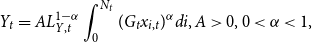 \begin{equation}Y_t=AL^{1-\alpha}_{Y,t} \int_0^{N_t} (G_t x_{i,t})^\alpha di, A>0, 0<\alpha<1, \end{equation}
where
 $Y_t$
is output,
$Y_t$
is output,
 $L_{Y,t}$
is labor input in the final goods sector, and
$L_{Y,t}$
is labor input in the final goods sector, and
 $x_{i,t}$
is the input of intermediate good i. Following Barro (Reference Barro1990), public services,
$x_{i,t}$
is the input of intermediate good i. Following Barro (Reference Barro1990), public services,
 $G_t$
, increase the productivity of output. We take the final output as the numeraire. Although
$G_t$
, increase the productivity of output. We take the final output as the numeraire. Although
 $\alpha$
encompasses both (i) the output elasticity of public services and (ii) the price elasticity of intermediate goods
$\alpha$
encompasses both (i) the output elasticity of public services and (ii) the price elasticity of intermediate goods
 $1/(1-\alpha)$
, we examine the former in this simple model. In the extended model (Section 5), we separate (i) and (ii). We denote the price of intermediate good i and wage rate as
$1/(1-\alpha)$
, we examine the former in this simple model. In the extended model (Section 5), we separate (i) and (ii). We denote the price of intermediate good i and wage rate as
 $p_{i,t}$
and
$p_{i,t}$
and
 $w_t$
, respectively. The profit maximization yields
$w_t$
, respectively. The profit maximization yields
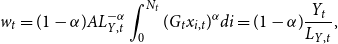 \begin{align}w_t&=(1-\alpha)AL_{Y,t}^{-\alpha} \int_0^{N_t} (G_t x_{i,t})^\alpha di=(1-\alpha)\frac{Y_t}{L_{Y,t}}, \end{align}
 \begin{align}p_{i,t}&=\alpha A L^{1-\alpha}_{Y,t}G_t^{\alpha}x^{\alpha-1}_{i,t}. \end{align}
Solving (2) and (3) with respect to
 $x_{i,t}$
yields the demand function for the product of firm i:
$x_{i,t}$
yields the demand function for the product of firm i:
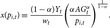 \begin{equation}x(p_{i,t})\equiv\frac{(1-\alpha)Y_t}{w_t}\Bigg(\frac{\alpha A G_t^\alpha}{p_{i,t}}\Bigg)^{\frac{1}{1-\alpha}}. \end{equation}
2.2 Producers of intermediate goods
2.2.1 Entry into the intermediate goods market
Each intermediate good is produced by a monopolistically competitive firm. To operate in period t, each intermediate good firm must invest
 $\eta$
unit of the final good in period
$\eta$
unit of the final good in period
 $t-1$
. Firms finance the cost of this investment by borrowing from households. Because firms must incur investment costs in each period, the planning horizon of each firm is one period, as in Young (Reference Young1998). When incurring investment costs, each firm draws its productivity
$t-1$
. Firms finance the cost of this investment by borrowing from households. Because firms must incur investment costs in each period, the planning horizon of each firm is one period, as in Young (Reference Young1998). When incurring investment costs, each firm draws its productivity
 $b>0 $
from distribution F(b). We assume that (i) b is independent and identically distributed (iid) over time as well as across firms and (ii) b is private information. These two assumptions are useful in describing an environment where the true tax base of each firm cannot be observable without auditing firms, as we explain in Sections 2.2.2 and 2.2.3. Besides, heterogeneity among firms’ productivity enables us to describe the realistic firm size distribution for the quantitative analysis in Section 5.
$b>0 $
from distribution F(b). We assume that (i) b is independent and identically distributed (iid) over time as well as across firms and (ii) b is private information. These two assumptions are useful in describing an environment where the true tax base of each firm cannot be observable without auditing firms, as we explain in Sections 2.2.2 and 2.2.3. Besides, heterogeneity among firms’ productivity enables us to describe the realistic firm size distribution for the quantitative analysis in Section 5.
Let us denote the expected after-tax operating profit of a firm with productivity b in period t by
 $ \pi^{e}_{i,t}$
.
$ \pi^{e}_{i,t}$
.
 $\pi^{e}_{i,t}$
depends on b. The next subsection discusses
$\pi^{e}_{i,t}$
depends on b. The next subsection discusses
 $ \pi^{e}_{i,t} $
in detail. The objective of intermediate good firm i that invests in period
$ \pi^{e}_{i,t} $
in detail. The objective of intermediate good firm i that invests in period
 $ t-1 $
is given by
$ t-1 $
is given by
 \begin{equation}\Pi_{i,t-1}=\frac{1}{R_{t-1}}\int \pi^{e}_{i,t} dF(b)-\eta, \end{equation}
where
 $R_{t-1}$
is the gross interest rate between periods
$R_{t-1}$
is the gross interest rate between periods
 $t-1$
and t. Since b is iid across firms, all firms face the same
$t-1$
and t. Since b is iid across firms, all firms face the same
 $ \Pi_{t-1} $
in period
$ \Pi_{t-1} $
in period
 $ t-1 $
. Free entry into the intermediate goods market implies
$ t-1 $
. Free entry into the intermediate goods market implies
 \begin{equation}\int \pi^e_{i,t}dF(b)=R_{t-1}\eta. \end{equation}
2.2.2 Expected operating profits
We assume that the price of each intermediate good
 $p_{i,t}$
is public information. A firm with productivity b needs
$p_{i,t}$
is public information. A firm with productivity b needs
 $1/b$
unit of labor to produce one unit of the intermediate good. The true operating profit of firm i is given by
$1/b$
unit of labor to produce one unit of the intermediate good. The true operating profit of firm i is given by
 \begin{equation} \pi_{i,t}=\left( p_{i,t}-\frac{w_t}{b_i}\right) x( p_{i,t}). \end{equation}
We use the word “true” to distinguish the true operating profit from the operating profit that firm i declares,
 $\tilde{\pi}_{i,t}$
, to the government. Because b is private information, the government cannot directly observe the true operating profit,
$\tilde{\pi}_{i,t}$
, to the government. Because b is private information, the government cannot directly observe the true operating profit,
 $ \pi_{i,t} $
, and thus, cannot know whether the declared profit (
$ \pi_{i,t} $
, and thus, cannot know whether the declared profit (
 $\tilde{\pi}_{i,t}$
) is equal to the true profit (
$\tilde{\pi}_{i,t}$
) is equal to the true profit (
 $\pi_{i,t}$
) without conducting an audit.
$\pi_{i,t}$
) without conducting an audit.
Denote the announced CIT rate by
 $\tau\in (0,1]$
. The after-tax profit of each firm is given by
$\tau\in (0,1]$
. The after-tax profit of each firm is given by
 $\pi_{i,t}-\tau \tilde{\pi}_{i,t}$
, because CIT is imposed on declared profit
$\pi_{i,t}-\tau \tilde{\pi}_{i,t}$
, because CIT is imposed on declared profit
 $ \tilde{\pi}_{i,t}$
. We denote the probability of an audit by
$ \tilde{\pi}_{i,t}$
. We denote the probability of an audit by
 $ {\bar q} \in [0,1]$
, and assume it is given exogenously. We impose a further assumption on
$ {\bar q} \in [0,1]$
, and assume it is given exogenously. We impose a further assumption on
 $ \bar{q} $
later. Suppose that a firm is audited. If this firm under-declares its operating profit (
$ \bar{q} $
later. Suppose that a firm is audited. If this firm under-declares its operating profit (
 $ \tilde{\pi}_{i,t} < \pi_{i,t} $
) to the government, it has to pay a penalty of
$ \tilde{\pi}_{i,t} < \pi_{i,t} $
) to the government, it has to pay a penalty of
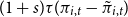 $ (1+s)\tau(\pi_{i,t}-\tilde{\pi}_{i,t} )$
, where the exogenous parameter
$ (1+s)\tau(\pi_{i,t}-\tilde{\pi}_{i,t} )$
, where the exogenous parameter
 $ s(\ge0) $
is an additional tax rate. If the firm over-declares its operating profit (
$ s(\ge0) $
is an additional tax rate. If the firm over-declares its operating profit (
 $ \tilde{\pi}_{i,t} > \pi_{i,t} $
), the overpayment,
$ \tilde{\pi}_{i,t} > \pi_{i,t} $
), the overpayment,
 $ \tau (\tilde{\pi}_{i,t}-\pi_{i,t}) $
, is refunded. The expected after-tax operating profit of firm i is given by
$ \tau (\tilde{\pi}_{i,t}-\pi_{i,t}) $
, is refunded. The expected after-tax operating profit of firm i is given by
 \begin{eqnarray*} \pi^e_{i,t}&=&\pi_{i,t}-\tau\tilde{\pi}_{i,t}-\bar{q}(1+s)\tau \cdot\max \{ 0, \ \pi_{i,t}-\tilde{\pi}_{i,t} \} + \bar{q} \tau \cdot\max \{ 0, \ \tilde{\pi}_{i,t}-\pi_{i,t} \}.\end{eqnarray*}
Given
 $ \pi_{i,t} $
,
$ \pi_{i,t} $
,
 $ \pi^e_{i,t} $
decreases with
$ \pi^e_{i,t} $
decreases with
 $ \tilde{\pi}_{i,t} $
if
$ \tilde{\pi}_{i,t} $
if
 $ \tilde{\pi}_{i,t} > \pi_{i,t} $
, and therefore no firms over-declare their operating profits, and the last term is equal to zero. Thus,
$ \tilde{\pi}_{i,t} > \pi_{i,t} $
, and therefore no firms over-declare their operating profits, and the last term is equal to zero. Thus,
 $ \tilde{\pi}_{i,t} \le \pi_{i,t} $
must be satisfied in the following discussion. Then, the expected after-tax operating profit,
$ \tilde{\pi}_{i,t} \le \pi_{i,t} $
must be satisfied in the following discussion. Then, the expected after-tax operating profit,
 $\pi^e_{i,t}$
, for
$\pi^e_{i,t}$
, for
 $ \tilde{\pi}_{i,t} \le \pi_{i,t}$
, is
$ \tilde{\pi}_{i,t} \le \pi_{i,t}$
, is
 \begin{equation}\pi^e_{i,t}=\pi_{i,t}-\tau\tilde{\pi}_{i,t}-\bar{q}(1+s)\tau( \pi_{i,t}-\tilde{\pi}_{i,t})=(1-\tilde{\tau})\pi_{i,t}, \end{equation}
where
 $\tilde{\tau}$
is the effective CIT rate and defined as
$\tilde{\tau}$
is the effective CIT rate and defined as
 \begin{equation}\tilde{\tau} \equiv \left\{[1-\bar{q}(1+s)]\frac{\tilde{\pi}_{i,t}}{\pi_{i,t}}+\bar{q}(1+s) \right\} \tau. \end{equation}
2.2.3 Tax evasion and maximization of the expected operating profits
Firm i chooses
 $\tilde{\pi}_{i,t}$
and
$\tilde{\pi}_{i,t}$
and
 $p_{i,t}$
to maximize
$p_{i,t}$
to maximize
 $\pi^{e}_{i,t}$
. Our specification of tax evasion behavior is essentially similar to that of Allingham and Sandmo (Reference Allingham and Sandmo1972), who consider tax evasion by a representative household, which evades income tax by choosing a declared income when its actual income is not directly known by the government. In our setting, each firm chooses its declared profit,
$\pi^{e}_{i,t}$
. Our specification of tax evasion behavior is essentially similar to that of Allingham and Sandmo (Reference Allingham and Sandmo1972), who consider tax evasion by a representative household, which evades income tax by choosing a declared income when its actual income is not directly known by the government. In our setting, each firm chooses its declared profit,
 $ \tilde{\pi}_{i,t}$
, by adjusting the price level when its actual profit,
$ \tilde{\pi}_{i,t}$
, by adjusting the price level when its actual profit,
 $\pi_{i,t}$
, is not directly known by the government.
$\pi_{i,t}$
, is not directly known by the government.
As a first step, we briefly discuss the case where the government can observe the true operating profits of each firm without any costs. We still assume that b is private information. Let us define the following function of p :
 \begin{align} \Lambda(p) = (1-\alpha) p x(p), \end{align}
where x(p) is defined by (4). Since the government can observe the true operating profits, each firm declares its profits truthfully. We substitute
 $ \tilde{\pi}_{i,t}=\pi_{i,t} $
into (8), which yields
$ \tilde{\pi}_{i,t}=\pi_{i,t} $
into (8), which yields
 $ \pi^e_{i,t}=(1-\tau)\pi_{i,t} $
. Thus,
$ \pi^e_{i,t}=(1-\tau)\pi_{i,t} $
. Thus,
 $ \pi^e_{i,t} $
is maximized at
$ \pi^e_{i,t} $
is maximized at
 $p_{i,t} = p^*_{i,t}$
, where
$p_{i,t} = p^*_{i,t}$
, where
 $p^\ast_{i,t}$
is defined as
$p^\ast_{i,t}$
is defined as
 $p^*_{i,t} \equiv \frac{w_t}{\alpha b_i}$
. The maximized operating profits is given by
$p^*_{i,t} \equiv \frac{w_t}{\alpha b_i}$
. The maximized operating profits is given by
 $ \Lambda( p^*_{i,t} ) $
. Since firm i declares truthfully, the declared profit
$ \Lambda( p^*_{i,t} ) $
. Since firm i declares truthfully, the declared profit
 $ \tilde{\pi}_{i,t} $
satisfies
$ \tilde{\pi}_{i,t} $
satisfies
 $ \tilde{\pi}_{i,t} = \Lambda( p^*_{i,t} ) $
. The following points should be noted. First, function
$ \tilde{\pi}_{i,t} = \Lambda( p^*_{i,t} ) $
. The following points should be noted. First, function
 $ \Lambda(p) $
does not depend on b. Thus, although b is not observable, the government knows the functional form of
$ \Lambda(p) $
does not depend on b. Thus, although b is not observable, the government knows the functional form of
 $ \Lambda(p) $
as long as it knows the demand function, (4). Second, since b is private information, the government cannot directly observe whether the price set by firm i,
$ \Lambda(p) $
as long as it knows the demand function, (4). Second, since b is private information, the government cannot directly observe whether the price set by firm i,
 $ p_{i,t} $
, is actually equal to
$ p_{i,t} $
, is actually equal to
 $ p^*_{i,t} = \frac{w_t}{\alpha b_i} $
. Finally, the above result suggests that if firm i declares truthfully, the price set by the firm,
$ p^*_{i,t} = \frac{w_t}{\alpha b_i} $
. Finally, the above result suggests that if firm i declares truthfully, the price set by the firm,
 $ p_{i,t} $
, and its declared profits,
$ p_{i,t} $
, and its declared profits,
 $ \tilde{\pi}_{i,t} $
, satisfy
$ \tilde{\pi}_{i,t} $
, satisfy
 $ \tilde{\pi}_{i,t} = \Lambda (p_{i,t}) $
. Conversely, if
$ \tilde{\pi}_{i,t} = \Lambda (p_{i,t}) $
. Conversely, if
 $ p_{i,t} $
and
$ p_{i,t} $
and
 $ \tilde{\pi}_{i,t} $
do not satisfy
$ \tilde{\pi}_{i,t} $
do not satisfy
 $ \tilde{\pi}_{i,t} = \Lambda (p_{i,t}) $
, firm i declares dishonestly.
$ \tilde{\pi}_{i,t} = \Lambda (p_{i,t}) $
, firm i declares dishonestly.
We now consider the case where the government cannot observe the true operating profits of each firm without any costs. We consider two subcases. First, assume that
 $ 1-\bar{q}(1+s)< 0 $
. We rewrite (8) as
$ 1-\bar{q}(1+s)< 0 $
. We rewrite (8) as
 \begin{align} \pi^e_{i,t}= [1-\bar{q}(1+s)\tau]\pi_{i,t}-[1-\bar{q}(1+s)]\tau \tilde{\pi}_{i,t}. \end{align}
If
 $1-\bar{q}(1+s)<0$
, firm i chooses
$1-\bar{q}(1+s)<0$
, firm i chooses
 $\tilde{\pi}_{i,t}=\pi_{i,t}$
because
$\tilde{\pi}_{i,t}=\pi_{i,t}$
because
 $\pi^e_{i,t}$
is increasing in
$\pi^e_{i,t}$
is increasing in
 $\tilde{\pi}_{i,t}$
. Then, each firm declares its profit truthfully. Thus, each firm sets
$\tilde{\pi}_{i,t}$
. Then, each firm declares its profit truthfully. Thus, each firm sets
 $ p_{i,t} =p^*_{i,t} $
. Furthermore,
$ p_{i,t} =p^*_{i,t} $
. Furthermore,
 $\tilde{\tau}=\tau$
by (9). Intuitively, if the expected additional tax rate is higher than the rate under honest declaration (
$\tilde{\tau}=\tau$
by (9). Intuitively, if the expected additional tax rate is higher than the rate under honest declaration (
 $\bar q(1+s)\tau> \tau$
), firms have no incentive to under-declare profits because CIT does not affect
$\bar q(1+s)\tau> \tau$
), firms have no incentive to under-declare profits because CIT does not affect
 $\tilde{\pi}_{i,t}$
. Thus, they declare true profits (
$\tilde{\pi}_{i,t}$
. Thus, they declare true profits (
 $\tilde{\pi}_{i,t}=\pi_{i,t}$
), and tax evasion does not occur.
$\tilde{\pi}_{i,t}=\pi_{i,t}$
), and tax evasion does not occur.
If
 $1-\bar{q}(1+s)=0$
, we obtain
$1-\bar{q}(1+s)=0$
, we obtain
 $\pi^e_{i,t}=(1-\tau)\pi_{i,t}$
by (11). In this case, the expected after-tax profit does not depend on whether a firm declares its profit truthfully. The maximization of
$\pi^e_{i,t}=(1-\tau)\pi_{i,t}$
by (11). In this case, the expected after-tax profit does not depend on whether a firm declares its profit truthfully. The maximization of
 $\pi^e_{i,t}=(1-\tau)\pi_{i,t}$
yields the same results as those of truth-telling firms. Summing up, we obtain the following.
$\pi^e_{i,t}=(1-\tau)\pi_{i,t}$
yields the same results as those of truth-telling firms. Summing up, we obtain the following.
Proposition 1. If
 $1-\bar{q}(1+s)\le0$
, then each firm i declares its true profit,
$1-\bar{q}(1+s)\le0$
, then each firm i declares its true profit,
 $\tilde{\pi}_{i,t}=\pi_{i,t}$
, and set its price level as
$\tilde{\pi}_{i,t}=\pi_{i,t}$
, and set its price level as
 $p_{i,t}=p^\ast_{i,t}$
. The effective CIT rate coincides with the announced CIT rate,
$p_{i,t}=p^\ast_{i,t}$
. The effective CIT rate coincides with the announced CIT rate,
 $\tilde{\tau}=\tau$
.
$\tilde{\tau}=\tau$
.
Next, we assume that
 $ 1-\bar{q}(1+s)> 0 $
. Then, (11) shows that
$ 1-\bar{q}(1+s)> 0 $
. Then, (11) shows that
 $\pi^e_{i,t}$
decreases with
$\pi^e_{i,t}$
decreases with
 $\tilde{\pi}_{i,t}$
. Thus, firm i has an incentive to under-declare its profits,
$\tilde{\pi}_{i,t}$
. Thus, firm i has an incentive to under-declare its profits,
 $ \tilde{\pi}^e_{i,t} < \pi^e_{i,t} $
. Remember that the government can observe the price set by firm i,
$ \tilde{\pi}^e_{i,t} < \pi^e_{i,t} $
. Remember that the government can observe the price set by firm i,
 $ p_{i,t} $
, and its declared operating profits,
$ p_{i,t} $
, and its declared operating profits,
 $ \tilde{\pi}_{i,t} $
, but cannot observe
$ \tilde{\pi}_{i,t} $
, but cannot observe
 $ b_i $
. This means that the government cannot observe whether firm i sets
$ b_i $
. This means that the government cannot observe whether firm i sets
 $ p_{i,t} $
according to
$ p_{i,t} $
according to
 $ p_{i,t} = \frac{w_t}{\alpha b_i} $
. Suppose that
$ p_{i,t} = \frac{w_t}{\alpha b_i} $
. Suppose that
 $ p_{i,t} $
and
$ p_{i,t} $
and
 $ \tilde{\pi}_{i,t} $
satisfy
$ \tilde{\pi}_{i,t} $
satisfy
 $\tilde{\pi}_{i,t} \neq \Lambda( p_{i,t} )$
, where function
$\tilde{\pi}_{i,t} \neq \Lambda( p_{i,t} )$
, where function
 $ \Lambda( \cdot ) $
is defined by (10). From the discussion in the paragraph that includes (10), the government knows that the firm declares dishonestly. In contrast, suppose that
$ \Lambda( \cdot ) $
is defined by (10). From the discussion in the paragraph that includes (10), the government knows that the firm declares dishonestly. In contrast, suppose that
 $ p_{i,t} $
and
$ p_{i,t} $
and
 $ \tilde{\pi}_{i,t} $
satisfy
$ \tilde{\pi}_{i,t} $
satisfy
 \begin{align} \tilde{\pi}_{i,t} = \Lambda( p_{i,t} ). \end{align}
Remember that the government cannot know whether the price set by firm i,
 $ p_{i,t} $
, is equal to
$ p_{i,t} $
, is equal to
 $ p^*_{i,t} =\frac{w_t}{\alpha b_i} $
. Thus, without auditing the firm, the government cannot know whether the firm declares truthfully. Given the discussion so far, we impose the following assumption.
$ p^*_{i,t} =\frac{w_t}{\alpha b_i} $
. Thus, without auditing the firm, the government cannot know whether the firm declares truthfully. Given the discussion so far, we impose the following assumption.
Assumption 1. Consider a firm that sets the price at
 $p_{i,t} $
. (i) If the firm’s declared profit satisfies
$p_{i,t} $
. (i) If the firm’s declared profit satisfies
 $ \tilde{\pi}_{i,t} \neq \Lambda( p_{i,t} ) $
, the firm is audited with a probability of one;
$ \tilde{\pi}_{i,t} \neq \Lambda( p_{i,t} ) $
, the firm is audited with a probability of one;
 $ \bar{q}=1 $
. (ii) If the firm’s declared profit satisfies
$ \bar{q}=1 $
. (ii) If the firm’s declared profit satisfies
 $ \tilde{\pi}_{i,t} = \Lambda( p_{i,t} ) $
, the firm is audited with a probability lower than one;
$ \tilde{\pi}_{i,t} = \Lambda( p_{i,t} ) $
, the firm is audited with a probability lower than one;
 $ \bar{q}=q \in[0,1) $
.
$ \bar{q}=q \in[0,1) $
.
This assumption captures the idea that if a firm unnaturally declares its profits, the government audits the firm. Under this assumption, we first demonstrate how each firm declares its profits in the following lemma.
Lemma. Suppose that
 $ 1-q(1+s)>0$
and that firm i sets
$ 1-q(1+s)>0$
and that firm i sets
 $ p_{i,t} $
. Then, its declared profit satisfies
$ p_{i,t} $
. Then, its declared profit satisfies
 $ \tilde{\pi}_{i,t} = \Lambda( p_{i,t} ) $
.
$ \tilde{\pi}_{i,t} = \Lambda( p_{i,t} ) $
.
Proof. See Appendix A.
Using Lemma, we consider firm i’s choice of the price level,
 $p_{i,t}$
.Footnote 12
$p_{i,t}$
.Footnote 12
Suppose that
 $ 1-q(1+s)> 0$
. Then, by (11),
$ 1-q(1+s)> 0$
. Then, by (11),
 $ \tilde{\pi}_{i,t} = \Lambda( p_{i,t} ) $
, and
$ \tilde{\pi}_{i,t} = \Lambda( p_{i,t} ) $
, and
 $\bar q =q$
, the problem of firm i is reduced to the problem to choose
$\bar q =q$
, the problem of firm i is reduced to the problem to choose
 $p_{i,t}$
to maximize
$p_{i,t}$
to maximize
 \begin{align*}\pi^e_{i,t}= [1-q(1+s)\tau]\left( p_{i,t}-\frac{w_t}{b_i}\right)x( p_{i,t})-[1-q(1+s)]\tau \Lambda(p_{i,t}),\end{align*}
subject to
 $p_{it}\geq p^\ast_{i,t}$
, which is from
$p_{it}\geq p^\ast_{i,t}$
, which is from
 $\tilde{\pi}_{i,t}\leq\pi_{i,t}$
.
$\tilde{\pi}_{i,t}\leq\pi_{i,t}$
.
The first-order condition is given by
 \begin{align}\frac{\partial \pi^e_{i,t}}{\partial p_{i,t}}&=[1-q(1+s)\tau]\frac{\partial\pi_{i,t}}{\partial p_{i,t}}-[1-q(1+s)]\tau \Lambda'(p_{i,t})\nonumber\\[5pt]&=\frac{\alpha x(p_{i,t})}{p_{i,t}} \left\{-\frac{1-q(1+s)\tau}{1-\alpha}\left(p_{i,t}-\frac{w_t}{\alpha b_i} \right)+[1-q(1+s)]\tau p_{i,t} \right\}=0, \end{align}
given that
 $\frac{\partial \pi_{i,t}}{\partial p_{i,t}}=-\alpha x(p_{i,t}) \left[\frac{p_{i,t}-w_t/(\alpha b_i)}{(1-\alpha)p_{i,t}} \right]$
and
$\frac{\partial \pi_{i,t}}{\partial p_{i,t}}=-\alpha x(p_{i,t}) \left[\frac{p_{i,t}-w_t/(\alpha b_i)}{(1-\alpha)p_{i,t}} \right]$
and
 $\Lambda'(p_{i,t})=-\alpha x(p_{i,t})$
. Because
$\Lambda'(p_{i,t})=-\alpha x(p_{i,t})$
. Because
 $ 1-q(1+s)>0 $
holds, we have that
$ 1-q(1+s)>0 $
holds, we have that
 $ 0< (1-\alpha)[1-q(1+s)]\tau < [1-q(1+s)]\tau < 1-q(1+s)\tau $
, which ensures the second-order condition. Solving (13) yields the following interior solution for
$ 0< (1-\alpha)[1-q(1+s)]\tau < [1-q(1+s)]\tau < 1-q(1+s)\tau $
, which ensures the second-order condition. Solving (13) yields the following interior solution for
 $p_{it} > w_t/\alpha b_i$
, which is denoted by
$p_{it} > w_t/\alpha b_i$
, which is denoted by
 $\tilde{p}_{i,t}$
:
$\tilde{p}_{i,t}$
:
 \begin{equation} \tilde{p}_{i,t} \equiv \frac{w_t}{\alpha b_i}\Gamma(\tau), \mbox{ where } \Gamma(\tau)\equiv \frac{1-q(1+s)\tau}{1-q(1+s)\tau-(1-\alpha)[1-q(1+s)]\tau} >1. \end{equation}
Because
 $ 1-q(1+s)>0 $
and
$ 1-q(1+s)>0 $
and
 $ (1-\alpha)[1-q(1+s)]\tau < 1-q(1+s)\tau $
, we have
$ (1-\alpha)[1-q(1+s)]\tau < 1-q(1+s)\tau $
, we have
 $ \Gamma(\tau)>1 $
and, hence,
$ \Gamma(\tau)>1 $
and, hence,
 $ \tilde{p}_{i,t} >w_t/(\alpha b_i) $
is satisfied.
$ \tilde{p}_{i,t} >w_t/(\alpha b_i) $
is satisfied.
The following proposition summarizes firm i’s choice in which tax evasion occurs.
Proposition 2. Suppose that
 $ 1-q(1+s)>0$
and that Assumption 1 holds. Firms with productivity
$ 1-q(1+s)>0$
and that Assumption 1 holds. Firms with productivity
 $ b_i $
set the price,
$ b_i $
set the price,
 $\tilde{p}_{i,t}$
, as (14). The declared profit satisfies (12). The true profit and the expected after-tax operating profit are, respectively, given by
$\tilde{p}_{i,t}$
, as (14). The declared profit satisfies (12). The true profit and the expected after-tax operating profit are, respectively, given by
 \begin{align} \pi_{i,t} &=\left(1-\alpha \Gamma(\tau)^{-1} \right) \tilde{p}_{i,t} x(\tilde{p}_{i,t}) > \tilde{\pi}_{i,t}, \end{align}
 \begin{align} \pi^e_{i,t} &=(1-\tilde{\tau})\left(1-\alpha \Gamma(\tau)^{-1} \right)\tilde{p}_{i,t} x(\tilde{p}_{i,t}). \end{align}
The inequality
 $ \pi_{i,t} > \tilde{\pi}_{i,t} $
in (15) indicates that all firms under-declare their operating profits. The effective CIT rate,
$ \pi_{i,t} > \tilde{\pi}_{i,t} $
in (15) indicates that all firms under-declare their operating profits. The effective CIT rate,
 $\tilde{\tau}\in \left(0,\frac{1+\alpha q(1+s)}{1+\alpha}\right]$
, satisfies that
$\tilde{\tau}\in \left(0,\frac{1+\alpha q(1+s)}{1+\alpha}\right]$
, satisfies that
 $\tilde{\tau} < \tau$
.
$\tilde{\tau} < \tau$
.
Proof. See the text and Appendix B.
Proposition 2 states that if the expected additional tax rate is lower than the rate under honest declaration (
 $q(1+s)<1$
), firms choose to evade CIT by under-declaring profits (
$q(1+s)<1$
), firms choose to evade CIT by under-declaring profits (
 $\tilde{\pi}_{i,t} < \pi_{i,t}$
). This is captured by
$\tilde{\pi}_{i,t} < \pi_{i,t}$
). This is captured by
 $\Gamma(\tau)$
, which is the only difference between the honest and dishonest declaration. Because
$\Gamma(\tau)$
, which is the only difference between the honest and dishonest declaration. Because
 $\Lambda'(p_{i,t})=-\alpha x (p_{i,t})<0$
, a firm can under-declare its profit by raising its price level. When firms under-declare profits, they pretend to be less productive, which leads to a higher price setting (
$\Lambda'(p_{i,t})=-\alpha x (p_{i,t})<0$
, a firm can under-declare its profit by raising its price level. When firms under-declare profits, they pretend to be less productive, which leads to a higher price setting (
 $\Gamma (\tau)>1$
), as represented by (14).
$\Gamma (\tau)>1$
), as represented by (14).
Notably, the CIT rate itself has a substantial effect on tax evasion through the term
 $\Gamma(\tau)$
. From (9) and (15), we have
$\Gamma(\tau)$
. From (9) and (15), we have
 $\mbox{sign} d(\tilde{\pi}_{i,t}/\pi_{i,t})/d\tau=\mbox{sign} d(\tilde{\tau}/\tau)/d\tau =\mbox{sign} d(1/\Gamma(\tau))/d\tau<0$
.Footnote 13 Thus, a rise in the CIT rate increases the difference between the true profit (
$\mbox{sign} d(\tilde{\pi}_{i,t}/\pi_{i,t})/d\tau=\mbox{sign} d(\tilde{\tau}/\tau)/d\tau =\mbox{sign} d(1/\Gamma(\tau))/d\tau<0$
.Footnote 13 Thus, a rise in the CIT rate increases the difference between the true profit (
 $\pi_{i,t}$
) and the declared profit (
$\pi_{i,t}$
) and the declared profit (
 $\tilde{\pi}_{i,t}$
) and encourages tax evasion.
$\tilde{\pi}_{i,t}$
) and encourages tax evasion.
Tax evasion by firms may not be possible if we assume that the government incorporates the equilibrium behavior of firms (14) and, thus, can infer productivity
 $b_i$
from
$b_i$
from
 $\tilde{p}_{i,t}$
. Although recent literature on optimal taxation using the mechanism design approach includes this assumption, we do not. Instead, we assume that a government does not conduct such a perfect back calculation, as in Allingham and Sandmo (Reference Allingham and Sandmo1972), because this simple setting allows us to provide interesting analyses on the macroeconomic consequences of CIT evasion in a tractable model.
$\tilde{p}_{i,t}$
. Although recent literature on optimal taxation using the mechanism design approach includes this assumption, we do not. Instead, we assume that a government does not conduct such a perfect back calculation, as in Allingham and Sandmo (Reference Allingham and Sandmo1972), because this simple setting allows us to provide interesting analyses on the macroeconomic consequences of CIT evasion in a tractable model.
REMARKS
The properties
 $d\tilde{\tau}/d\tau>0$
and
$d\tilde{\tau}/d\tau>0$
and
 $d(\tilde{\tau}/\tau)/d\tau < 0$
are in line with Roubini and Sala-i-Martin (Reference Roubini1995) and Kafkalas et al. (Reference Kafkalas, Kalaitzidakis and Tzouvelekas2014).Footnote 14 However, the tax evasion considered in our model departs from these previous studies in the following respects.
$d(\tilde{\tau}/\tau)/d\tau < 0$
are in line with Roubini and Sala-i-Martin (Reference Roubini1995) and Kafkalas et al. (Reference Kafkalas, Kalaitzidakis and Tzouvelekas2014).Footnote 14 However, the tax evasion considered in our model departs from these previous studies in the following respects.
First, tax evasion in our model is derived endogenously from the micro foundation of firms’ tax evasion behavior, in contrast to the ad-hoc expression by Roubini and Sala-i-Martin (Reference Roubini1995).
Second, Chen (Reference Chen2003) and Kafkalas et al. (Reference Kafkalas, Kalaitzidakis and Tzouvelekas2014) do not consider tax evasion associated with profit maximization in an imperfectly competitive product market. Thus, there is no relationship between the tax rates and the firms’ choice of profits and declarations of profits in their models. In contrast, in our model, the CIT rate affects them substantially, as represented by
 $\Gamma(\tau)>1$
and
$\Gamma(\tau)>1$
and
 $\Gamma'(\tau)>0$
.
$\Gamma'(\tau)>0$
.
2.3 Household
The population size is constant at one. The utility function of a representative household is
 \begin{equation}U_0=\sum_{t=0}^{\infty}\left(\frac{1}{1+\rho}\right)^t u(C_t), u(C_t)=\frac{C^{1-\sigma}_t}{1-\sigma}, \ \ \sigma>0. \end{equation}
 $u(C_t)=\ln{C_t}$
, when
$u(C_t)=\ln{C_t}$
, when
 $\sigma=1$
. Here,
$\sigma=1$
. Here,
 $C_t$
,
$C_t$
,
 $\rho(>0)$
and
$\rho(>0)$
and
 $1/\sigma$
denote consumption in period t, the subjective discount rate, and the intertemporal elasticity of substitution, respectively. The representative household supplies L unit of labor inelastically. The household’s budget constraint is given by
$1/\sigma$
denote consumption in period t, the subjective discount rate, and the intertemporal elasticity of substitution, respectively. The representative household supplies L unit of labor inelastically. The household’s budget constraint is given by
 $W_{t}=R_{t-1}W_{t-1} +w_t L -C_t$
, where
$W_{t}=R_{t-1}W_{t-1} +w_t L -C_t$
, where
 $W_{t-1}$
is the assets at the end of period
$W_{t-1}$
is the assets at the end of period
 $t-1$
. The household’s utility maximization yields
$t-1$
. The household’s utility maximization yields
 \begin{equation}\frac{C_{t+1}}{C_{t}}=\left(\frac{R_t}{1+\rho} \right)^{1/\sigma}, \end{equation}
and the transversality condition (TVC) is
 \begin{equation}\lim_{t \rightarrow \infty}\frac{ C^{-\sigma}_t W_{t-1}}{(1+\rho)^t}=0. \end{equation}
2.4 Government
We assume that the government keeps a balanced budget in each period. From (8) and (9), the aggregate tax revenue of the government is
 $\int_0^{N_t}\int \{\tau\tilde{\pi}_{i,t}+q(1+s)\tau[\pi_{i,t}-\tilde{\pi}_{i,t}]\}dF(b)di=\tilde{\tau} \int_0^{N_t}\int \pi_{i,t}dF(b)di= \tilde{\tau} N_t\int \pi_{i,t}dF(b)$
. Here, we use the fact that b is iid across firms. This revenue is allocated to productive government spending,
$\int_0^{N_t}\int \{\tau\tilde{\pi}_{i,t}+q(1+s)\tau[\pi_{i,t}-\tilde{\pi}_{i,t}]\}dF(b)di=\tilde{\tau} \int_0^{N_t}\int \pi_{i,t}dF(b)di= \tilde{\tau} N_t\int \pi_{i,t}dF(b)$
. Here, we use the fact that b is iid across firms. This revenue is allocated to productive government spending,
 $G_t$
, and inspection expenditure to detect tax evasion,
$G_t$
, and inspection expenditure to detect tax evasion,
 $M_t$
. Thus, the budget constraint of the government is given by
$M_t$
. Thus, the budget constraint of the government is given by
 \begin{equation} \tilde{\tau} N_t \int \pi_{i,t} dF(b)=G_t + M_t. \end{equation}
The probability of a successful detection of tax evasion by a firm q occurs when we assume spending a constant fraction, Q, of government revenue on
 $M_t$
.Footnote 15 Therefore, the inspection expenditure is given by
$M_t$
.Footnote 15 Therefore, the inspection expenditure is given by
 $ M_t =Q \tilde{\tau} N_t \int \pi_{i,t} dF(b) $
. This specification of
$ M_t =Q \tilde{\tau} N_t \int \pi_{i,t} dF(b) $
. This specification of
 $M_t$
is in line with Kafkalas et al. (Reference Kafkalas, Kalaitzidakis and Tzouvelekas2014). Thus, (20) reduces to
$M_t$
is in line with Kafkalas et al. (Reference Kafkalas, Kalaitzidakis and Tzouvelekas2014). Thus, (20) reduces to
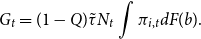 \begin{equation}G_t=(1-Q)\tilde{\tau} N_t \int \pi_{i,t} dF(b). \end{equation}
As mentioned in the Introduction section, such a specification allows us to isolate the role of tax evasion by firms with market power for pursuing Barro’s rule. This is because Kafkalas et al.’s (Reference Kafkalas, Kalaitzidakis and Tzouvelekas2014) result indicate that Barro’s rule holds even with the tax evasion of perfectly competitive firms under inspection expenditure of the form in (21).
3. Equilibrium
An equilibrium is an allocation in which (i) all monopolistically competitive firms choose
 $[p_{i,t}, x_{i,t}]^{\infty}_{t=0}$
, for
$[p_{i,t}, x_{i,t}]^{\infty}_{t=0}$
, for
 $i\in[0, N_t]$
, to maximize their after-tax operating profits; (ii) the evolution of the varieties of intermediate goods,
$i\in[0, N_t]$
, to maximize their after-tax operating profits; (ii) the evolution of the varieties of intermediate goods,
 $[N_t]^{\infty}_{t=0}$
, is determined by free entry; (iii) the evolution of net interest and wage rates,
$[N_t]^{\infty}_{t=0}$
, is determined by free entry; (iii) the evolution of net interest and wage rates,
 $[R_{t-1}, w_t ]^{\infty}_{t=0}$
, satisfy market clearing; (iv) the evolution of aggregate consumption and investment,
$[R_{t-1}, w_t ]^{\infty}_{t=0}$
, satisfy market clearing; (iv) the evolution of aggregate consumption and investment,
 $[C_t, \eta N_{t+1}]^\infty_{t=0}$
, is consistent with a household’s utility maximization; and (v) the evolution of productive public expenditures and inspection expenditures,
$[C_t, \eta N_{t+1}]^\infty_{t=0}$
, is consistent with a household’s utility maximization; and (v) the evolution of productive public expenditures and inspection expenditures,
 $[G_t,M_t]^\infty_{t=0}$
, satisfy the budget constraint of the government, taking the announced CIT rate, additional tax rate, and the probability of an audit,
$[G_t,M_t]^\infty_{t=0}$
, satisfy the budget constraint of the government, taking the announced CIT rate, additional tax rate, and the probability of an audit,
 $(\tau,s,q )$
, as given.
$(\tau,s,q )$
, as given.
We begin with the labor market, which clears as
 \begin{equation} L=L_{Y,t} +N_t\int \frac{x_{i,t}}{b}dF(b). \end{equation}
The cost for entry into the intermediate good market
 $ \eta $
is financed by borrowing from households. Because
$ \eta $
is financed by borrowing from households. Because
 $ N_{t+1} $
firms invest in period t, the asset market equilibrium condition is given by
$ N_{t+1} $
firms invest in period t, the asset market equilibrium condition is given by
 $W_{t} =\eta N_{t+1}$
. The final good market clears as
$W_{t} =\eta N_{t+1}$
. The final good market clears as
 $Y_t =C_t + \eta N_{t+1} +G_t +M_t$
.
$Y_t =C_t + \eta N_{t+1} +G_t +M_t$
.
We next characterize the dynamic system and the steady state of the economy. Appendix D shows that the dynamic system of the economy is characterized by the following single difference equation with respect to
 $z_t\equiv C_t/N_t$
:
$z_t\equiv C_t/N_t$
:
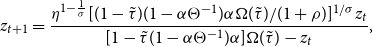 \begin{equation}z_{t+1}=\frac{ \eta^{1-\frac{1}{\sigma}} [(1-\tilde{\tau})(1-\alpha\Theta^{-1})\alpha \Omega(\tilde{\tau})/(1+\rho) ]^{1/\sigma} z_t}{[1-\tilde{\tau}(1-\alpha\Theta^{-1})\alpha]\Omega(\tilde{\tau}) -z_t }, \end{equation}
where
 \begin{equation*}\Theta=\begin{cases}1 & \text {if $1-q(1+s)\leq 0$}\\[5pt]\Gamma(\tau) & \text {if $1-q(1+s)>0$},\\\end{cases}\end{equation*}
and
 $\Omega(\tilde{\tau})$
in (23) is
$\Omega(\tilde{\tau})$
in (23) is
 $Y_t/N_t$
and is constant over time:
$Y_t/N_t$
and is constant over time:
 \begin{align}\frac{Y_t}{N_t}\left(=\frac{Y_{t+1}}{N_{t+1}}\right)=\Omega(\tilde{\tau})\equiv&A^{\frac{1}{1-\alpha}}\left[(1-Q)\tilde{\tau}\left(1-\alpha \Theta^{-1} \right)\alpha \right]^{\frac{\alpha}{1-\alpha}} (1-\alpha)\Theta \alpha^{\frac{2\alpha}{1-\alpha}} \nonumber\\&\times\left[\frac{L}{(1-\alpha)\Theta+\alpha^2}\right]^{\frac{1}{1-\alpha}}\left[\int b^{\frac{\alpha}{1-\alpha}} dF(b)\right]. \end{align}
Here, note that since
 $Y_t/N_t$
is constant,
$Y_t/N_t$
is constant,
 $G_tx_{i,t}$
in (1) is also constant on the balanced growth path. Thus, because
$G_tx_{i,t}$
in (1) is also constant on the balanced growth path. Thus, because
 $G_t/N_t$
is constant by (21), the growth rate of
$G_t/N_t$
is constant by (21), the growth rate of
 $x_{i,t}$
is
$x_{i,t}$
is
 $-\hat{g}$
, where
$-\hat{g}$
, where
 $\hat{g}$
is the growth rate in the steady state defined in Proposition 3 below. So that the individual intermediate good firms’ revenues and their profits do not grow at the balanced growth path. However, the economy grows by the expansion of varieties, the increase in
$\hat{g}$
is the growth rate in the steady state defined in Proposition 3 below. So that the individual intermediate good firms’ revenues and their profits do not grow at the balanced growth path. However, the economy grows by the expansion of varieties, the increase in
 $N_t$
: See (1).
$N_t$
: See (1).
From (23), we arrive at the following proposition.
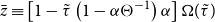
Proposition 3. A unique steady state exists. In the steady state,
 $z_t$
takes the following constant value:
$z_t$
takes the following constant value:
 \begin{align}\hat{z}=\left[1-\tilde{\tau}\left(1-\alpha\Theta^{-1}\right)\alpha \right]\Omega(\tilde{\tau})-\eta\left[ (1-\tilde{\tau})\left(1-\alpha\Theta^{-1} \right) \alpha(1+\rho)^{-1}\eta^{-1} \Omega(\tilde{\tau}) \right]^{1/\sigma}\in (0, \bar{z}),\nonumber\\ \end{align}
where
 $\bar{z}\equiv\left[1-\tilde{\tau}\left(1-\alpha\Theta^{-1}\right)\alpha \right]\Omega(\tilde{\tau})$
. In the steady state,
$\bar{z}\equiv\left[1-\tilde{\tau}\left(1-\alpha\Theta^{-1}\right)\alpha \right]\Omega(\tilde{\tau})$
. In the steady state,
 $C_t$
,
$C_t$
,
 $N_t$
, and
$N_t$
, and
 $Y_t$
grow at the same constant rate:
$Y_t$
grow at the same constant rate:
 \begin{align}\hat{g}=\left[ (1-\tilde{\tau})\left(1-\alpha\Theta^{-1} \right) \alpha(1+\rho)^{-1}\eta^{-1} \Omega(\tilde{\tau}) \right]^{1/\sigma}. \end{align}
The economy jumps to the steady state initially.
Proof. See Appendix E.
The labor allocated to the production of final and intermediate goods,
 $ L_{Y,t} $
and
$ L_{Y,t} $
and
 $ N_t\int \frac{x_{i,t}}{b}dF(b) $
, are both constant over time during the steady state. In addition,
$ N_t\int \frac{x_{i,t}}{b}dF(b) $
, are both constant over time during the steady state. In addition,
 $ Y_t $
,
$ Y_t $
,
 $ C_t $
,
$ C_t $
,
 $ G_t $
, and
$ G_t $
, and
 $ M_t $
grow at the same rate as
$ M_t $
grow at the same rate as
 $ N_t $
. Again, note that the source of economic growth in our model is firms’ investment in a new business (
$ N_t $
. Again, note that the source of economic growth in our model is firms’ investment in a new business (
 $N_{t+1}$
), as in the standard expanding variety model, which becomes the fundamental source of perpetual growth. In addition, productive government service (
$N_{t+1}$
), as in the standard expanding variety model, which becomes the fundamental source of perpetual growth. In addition, productive government service (
 $G_t$
) has a growth effect. It amplifies the demand for intermediate goods, increases the expected profits of the intermediate good firms, promotes their entry, and raises the interest rate through the free entry condition: See (4) and (6). We investigate this growth effect in greater detail in the next section.
$G_t$
) has a growth effect. It amplifies the demand for intermediate goods, increases the expected profits of the intermediate good firms, promotes their entry, and raises the interest rate through the free entry condition: See (4) and (6). We investigate this growth effect in greater detail in the next section.
4. Optimal CIT rates
As mentioned in Section 2, the CIT rate substantially affects the tax evasion behavior of firms in the imperfectly competitive market. Therefore, we analyze the growth- and welfare-maximizing CIT rates under such CIT evasion.Footnote 16
4.1 Growth-maximizing CIT rate
We obtain the following proposition.
Proposition 4. Let us denote the growth-maximizing announced CIT rate and growth-maximizing effective CIT rate as
 $\tau^{GM}$
and
$\tau^{GM}$
and
 $\tilde{\tau}^{GM}$
, respectively.
$\tilde{\tau}^{GM}$
, respectively.
-
1. When
 $1-q(1+s)\leq 0$
and each firm declares its true operating profit,
$\tilde{\tau}^{GM}=\tau^{GM}=\alpha$
holds.
$1-q(1+s)\leq 0$
and each firm declares its true operating profit,
$\tilde{\tau}^{GM}=\tau^{GM}=\alpha$
holds. -
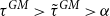
2. When
$1-q(1+s)>0$
and each firm under-declares its operating profit,
$\tau^{GM}> \tilde{\tau}^{GM}>\alpha$
holds.


Proof. See Appendix F.
The first part of Proposition 4 is in line with Barro’s (Reference Barro1990) rule, that is, the tax rate that maximizes long-run growth equals the output elasticity of public services,
 $\alpha$
. This result is also consistent with that of Kafkalas et al. (Reference Kafkalas, Kalaitzidakis and Tzouvelekas2014), indicating that even with government spending for detection, the growth-maximizing tax rate coincides with the output elasticity of public services.
$\alpha$
. This result is also consistent with that of Kafkalas et al. (Reference Kafkalas, Kalaitzidakis and Tzouvelekas2014), indicating that even with government spending for detection, the growth-maximizing tax rate coincides with the output elasticity of public services.
Importantly, the mechanism behind this result is the same as that of Barro (Reference Barro1990). In Barro’s model, the growth-maximizing rule is attributed to the following trade-off between income tax and growth. Meanwhile, an increase in income tax decreases the net interest rate ((1
 $- $
tax rate)
$- $
tax rate)
 $\times$
interest rate) and hurts growth, and an increase in income tax boosts productive government spending and raises the interest rate. This has a positive effect on growth.
$\times$
interest rate) and hurts growth, and an increase in income tax boosts productive government spending and raises the interest rate. This has a positive effect on growth.
The interest rate in our model is determined through the free entry condition of intermediate goods firms as
 \begin{equation}R_{t-1}=\eta^{-1}\int \pi^{e}_{i,t}dF(b)=\eta^{-1}(1-\tilde{\tau})(1-\alpha\Theta^{-1})\alpha Y_t/N_t. \end{equation}
Here,
 $Y_t/N_t$
, given in (24), is positively affected byFootnote 17
$Y_t/N_t$
, given in (24), is positively affected byFootnote 17
 \begin{equation}G_t=(1-Q)\tilde{\tau} N_t \int \pi_{i,t}dF(b)=(1-Q)\tilde{\tau}(1-\alpha\Theta^{-1})\alpha Y_t. \end{equation}
This induces essentially the same trade-off as Barro (Reference Barro1990). Thus, in the absence of tax evasion (
 $\Theta=1$
), we obtain the same result as Barro (Reference Barro1990).
$\Theta=1$
), we obtain the same result as Barro (Reference Barro1990).
The second part of Proposition 4 states that with under-declaration of profit, the growth-maximizing announced CIT rate is higher than the growth-maximizing effective CIT rate,
 $\tau^{GM}>\tilde{\tau}^{GM}$
. Moreover, both are higher than the output elasticity of public services,
$\tau^{GM}>\tilde{\tau}^{GM}$
. Moreover, both are higher than the output elasticity of public services,
 $\alpha$
. That is, tax evasion by firms increases the growth-maximizing tax rates,
$\alpha$
. That is, tax evasion by firms increases the growth-maximizing tax rates,
 $\tau^{GM}$
and
$\tau^{GM}$
and
 $\tilde{\tau}^{GM}$
.
$\tilde{\tau}^{GM}$
.
 $\tau^{GM}>\tilde{\tau}^{GM}$
stems simply from the evasion of CIT by firms. Then, we consider the intuition behind the result of
$\tau^{GM}>\tilde{\tau}^{GM}$
stems simply from the evasion of CIT by firms. Then, we consider the intuition behind the result of
 $\tilde{\tau}^{GM}>\alpha$
here.
$\tilde{\tau}^{GM}>\alpha$
here.
As we have seen after Proposition 2, in response to a tax hike, each intermediate good firm increases tax evasion. This secures the expected operating after-tax profit,
 $\pi^{e}_{i,t}$
, and private investment. Because the true operating profit,
$\pi^{e}_{i,t}$
, and private investment. Because the true operating profit,
 $\pi_{i,t}$
, is also secured, the tax base for public service provision (
$\pi_{i,t}$
, is also secured, the tax base for public service provision (
 $=N_t \int \pi_{i,t}dF(b)$
) is maintained.Footnote 18 These are caused by the effect of CIT evasion associated with profit maximization in an imperfectly competitive product market, which are captured by the term
$=N_t \int \pi_{i,t}dF(b)$
) is maintained.Footnote 18 These are caused by the effect of CIT evasion associated with profit maximization in an imperfectly competitive product market, which are captured by the term
 $1-\alpha\Theta^{-1}$
in (27) and (28), where
$1-\alpha\Theta^{-1}$
in (27) and (28), where
 $\Theta=\Gamma(\tau)$
and
$\Theta=\Gamma(\tau)$
and
 $\Gamma'(\tau)>0$
. Hereafter, we call this simply the effect of CIT evasion. The effect of CIT evasion mitigates the negative effect of CIT on growth and increases the benefit of raising the CIT rate for the provision of productive public services.Footnote 19
$\Gamma'(\tau)>0$
. Hereafter, we call this simply the effect of CIT evasion. The effect of CIT evasion mitigates the negative effect of CIT on growth and increases the benefit of raising the CIT rate for the provision of productive public services.Footnote 19
Our result (
 $\tilde{\tau}^{GM}>\alpha$
) is different from Kafkalas et al. (Reference Kafkalas, Kalaitzidakis and Tzouvelekas2014), who advocate that Barro’s rule holds (
$\tilde{\tau}^{GM}>\alpha$
) is different from Kafkalas et al. (Reference Kafkalas, Kalaitzidakis and Tzouvelekas2014), who advocate that Barro’s rule holds (
 $\tilde{\tau}^{GM}=\alpha$
) even in the economy with tax evasion. While tax evasion does not affect firms’ decision making in Kafkalas et al. (Reference Kafkalas, Kalaitzidakis and Tzouvelekas2014), our model includes the effect of CIT evasion as mentioned above, which causes
$\tilde{\tau}^{GM}=\alpha$
) even in the economy with tax evasion. While tax evasion does not affect firms’ decision making in Kafkalas et al. (Reference Kafkalas, Kalaitzidakis and Tzouvelekas2014), our model includes the effect of CIT evasion as mentioned above, which causes
 $\tilde{\tau}^{GM}>\alpha$
.Footnote 20
$\tilde{\tau}^{GM}>\alpha$
.Footnote 20
4.2 Welfare-maximizing CIT rate
Next, we analyze the welfare-maximizing CIT rate. Using the balanced growth rate,
 $\hat g$
, the equilibrium path of consumption is given by
$\hat g$
, the equilibrium path of consumption is given by
 $C_t=\hat g^t C_0=\hat g^t \hat{z}$
.Footnote 21 Substituting it into the lifetime utility function of the representative household, (17), we obtain
$C_t=\hat g^t C_0=\hat g^t \hat{z}$
.Footnote 21 Substituting it into the lifetime utility function of the representative household, (17), we obtain
 \begin{equation}U_0 = \frac{\hat{z}^{1-\sigma}}{(1-\sigma)\left[1-(1+\rho)^{-1}\hat g^{1-\sigma}\right]},\end{equation}
where
 $1>(1+\rho)^{-1}\hat g^{1-\sigma}$
holds by the TVC. The social welfare is determined by the initial level of consumption and the long-run growth rate, both of which depend on the announced CIT rate,
$1>(1+\rho)^{-1}\hat g^{1-\sigma}$
holds by the TVC. The social welfare is determined by the initial level of consumption and the long-run growth rate, both of which depend on the announced CIT rate,
 $\tau$
. Let us denote the welfare-maximizing announced CIT rate by
$\tau$
. Let us denote the welfare-maximizing announced CIT rate by
 $\tau^{WM}$
.
$\tau^{WM}$
.
Proposition 5.
-
1. When each firm declares its true operating profit,
$1-q(1+s)\leq 0$
,
$\tau^{WM}>\tau^{GM}=\alpha$
holds. Therefore, the welfare-maximizing announced CIT rate,
$\tau^{WM}$
, is higher than the growth-maximizing announced CIT rate,
$\tau^{GM}$
. -
2. Suppose that
$1-q(1+s)>0 $
and
$q=0$
. Then, each firm understates its operating profit and a marginal increase in the announced CIT rate at the growth-maximizing CIT rate improves social welfare.


Proof. See Appendix G.
Proposition 5 shows that the welfare-maximizing CIT is higher than the growth-maximizing one.Footnote 22 Meanwhile, a marginal increase in CIT from
 $\tau^{GM}$
does not affect the growth rate because the first-order effect vanishes at
$\tau^{GM}$
does not affect the growth rate because the first-order effect vanishes at
 $\tau=\tau^{GM}$
. In addition, it increases current consumption because labor income, which is exempt from taxation, is raised by increases in productive public services (see Appendix G). Therefore, the welfare-maximizing CIT rate is higher than the growth-maximizing one.
$\tau=\tau^{GM}$
. In addition, it increases current consumption because labor income, which is exempt from taxation, is raised by increases in productive public services (see Appendix G). Therefore, the welfare-maximizing CIT rate is higher than the growth-maximizing one.
5. Quantitative analysis
Propositions 4 and 5 summarize that the following three effects make
 $\tau^{WM}$
larger than the output elasticity of public services with tax evasion by firms (
$\tau^{WM}$
larger than the output elasticity of public services with tax evasion by firms (
 $1-q(1+s)>0$
).
$1-q(1+s)>0$
).
The first effect is represented by
 $\tau^{WM} > \tau^{GM}$
; the welfare-maximizing announced tax rate is higher than the growth-maximizing one. This is because the tax base is CIT, and wage income is exempt from taxation as we have seen in Proposition 5. We call this the tax base effect. The second effect is represented by
$\tau^{WM} > \tau^{GM}$
; the welfare-maximizing announced tax rate is higher than the growth-maximizing one. This is because the tax base is CIT, and wage income is exempt from taxation as we have seen in Proposition 5. We call this the tax base effect. The second effect is represented by
 $\tau^{GM}>\tilde{\tau}^{GM}$
. This stems from the degree of tax evasion by firms, (
$\tau^{GM}>\tilde{\tau}^{GM}$
. This stems from the degree of tax evasion by firms, (
 $\tau>\tilde{\tau}$
). We call this the difference in tax rates. The third effect is represented by
$\tau>\tilde{\tau}$
). We call this the difference in tax rates. The third effect is represented by
 $\tilde{\tau}^{GM}>\alpha$
. This is attributable to the effect of CIT evasion, as mentioned in Section 4.1
$\tilde{\tau}^{GM}>\alpha$
. This is attributable to the effect of CIT evasion, as mentioned in Section 4.1
The objective of this section is to investigate how high the welfare-maximizing CIT rate
 $\tau^{WM}$
is and which of the three effects contributes most to it. To solve these quantitative problems, we extend the above base model in this section.
$\tau^{WM}$
is and which of the three effects contributes most to it. To solve these quantitative problems, we extend the above base model in this section.
5.1 Extended model
We start with a small revision of the model because the problematic restriction on the parameter lies in the previous form of production technology. The output-elasticity of public services
 $\alpha$
must be set at the price elasticity of intermediate good,
$\alpha$
must be set at the price elasticity of intermediate good,
 $1/(1-\alpha)$
. To resolve this, we change production technology (1) into
$1/(1-\alpha)$
. To resolve this, we change production technology (1) into
 \begin{equation}Y_t=AL^{1-\alpha}_{Y,t} \int_0^{N_t} (a(G_t,N_t) x_{i,t})^\alpha di, \end{equation}
where
 \begin{equation}a(G_t,N_t)=G^{\epsilon}_t N^{1-\epsilon}_t, 0<\epsilon<1. \end{equation}
The composite externality (31) represents a combination of the role of knowledge spillover, as in Benassy (Reference Benassy1998), together with productive public services, as in Barro (Reference Barro1990).
We adopt this form of composite externality for the following two reasons: First, as will become evident below and as stated by Chatterjee and Turnovsky (Reference Chatterjee and Turnovsky2012), it helps to provide a plausible calibration of the aggregate economy, something that is generically problematic in the conventional one-sector endogenous growth model.Footnote 23 Under (30) and (31), the output-elasticity of public services is
 $\beta\equiv \alpha\epsilon ({<}\alpha)$
, which differentiates
$\beta\equiv \alpha\epsilon ({<}\alpha)$
, which differentiates
 $\alpha$
from the output-elasticity of public services. Notice that the specification of (30) and (31) is consistent with the existence of the balanced growth by the expanding varieties. Similarly, to the explanation right before Proposition 3,
$\alpha$
from the output-elasticity of public services. Notice that the specification of (30) and (31) is consistent with the existence of the balanced growth by the expanding varieties. Similarly, to the explanation right before Proposition 3,
 $G^{\epsilon}_t N^{1-\epsilon}_t x_{i,t}$
in (30) is constant on the balanced growth path. This means that the engine of growth in this extended model is also the expansion of varieties. Second, as the following Remark shows, although we take an additional externality (the spillover of knowledge) into account, the basic property of the benchmark model is maintained.
$G^{\epsilon}_t N^{1-\epsilon}_t x_{i,t}$
in (30) is constant on the balanced growth path. This means that the engine of growth in this extended model is also the expansion of varieties. Second, as the following Remark shows, although we take an additional externality (the spillover of knowledge) into account, the basic property of the benchmark model is maintained.
Remark. The qualitative results do not change in the extended model. By replacing
 $\alpha$
with
$\alpha$
with
 $\beta$
, the same results as Propositions 4 and 5 hold.
$\beta$
, the same results as Propositions 4 and 5 hold.
Proof: See Appendix H.
5.2 Calibration
To conduct numerical exercises, we set the baseline parameter value as in Table 1. Appendix I provides details of our calibration.
Table 1. Baseline parameter value
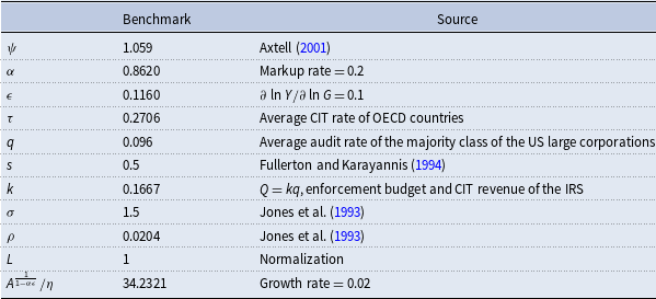
The distribution of firms’ productivity is determined to make the curvature of the distribution function of firm sizes in the model equal to that of the Pareto distribution estimated with US data by Axtell (Reference Axtell2001). This requires
 $\psi=$
1.059. We choose
$\psi=$
1.059. We choose
 $\alpha =$
0.8620 so that the markup rate of firms
$\alpha =$
0.8620 so that the markup rate of firms
 $\mu$
(
$\mu$
(
 $=\Gamma(\tau)/\alpha-1$
) takes 20%, which is a standard value of markup rate of firms (e.g., Rotemberg and Woodford (Reference Rotemberg and Woodford1999)).
$=\Gamma(\tau)/\alpha-1$
) takes 20%, which is a standard value of markup rate of firms (e.g., Rotemberg and Woodford (Reference Rotemberg and Woodford1999)).
We set the parameter to measure the knowledge spillover,
 $\epsilon$
, to 0.1160, so that the output elasticity of public services,
$\epsilon$
, to 0.1160, so that the output elasticity of public services,
 $\beta$
, equals 0.1. Although the estimates of the elasticity vary among some empirical studies, 0.1 is one of the reasonable values of
$\beta$
, equals 0.1. Although the estimates of the elasticity vary among some empirical studies, 0.1 is one of the reasonable values of
 $\beta$
.Footnote 24
$\beta$
.Footnote 24
In this subsection, we provide the baseline value of the announced CIT rate,
 $\tau=$
0.2706, to determine the baseline balanced growth rate because the balanced growth rate depends on
$\tau=$
0.2706, to determine the baseline balanced growth rate because the balanced growth rate depends on
 $\tau$
in this model economy. This value of
$\tau$
in this model economy. This value of
 $\tau$
(= 0.2706) is the average CIT rate in OECD countries from 2000 to 2017.Footnote 25 We set the penalty tax rate, s, to
$\tau$
(= 0.2706) is the average CIT rate in OECD countries from 2000 to 2017.Footnote 25 We set the penalty tax rate, s, to
 $0.5$
, according to Fullerton and Karayannis (Reference Fullerton and Karayannis1994), who take this value as a normal rate in the USA.
$0.5$
, according to Fullerton and Karayannis (Reference Fullerton and Karayannis1994), who take this value as a normal rate in the USA.
We set the benchmark value of the audit rate, q, to
 $0.096$
. To obtain this value, we utilize the statistics provided by the Internal Revenue Service. Each IRS Data Book between 2000 and 2017 provides the actual ratio of the examined corporations to all corporations under a classification by firm size.Footnote 26 We choose the class of the smallest size of the large corporations.Footnote 27 This is because such a class occupies a significantly large part (about 60%) of the large corporations, which are corporations above a certain business size. Besides, the ratios of the audited corporations vary greatly across the classes and so does the number of corporations in the classes. This means that taking the average audit rate among the classes is unreasonable. Therefore, we set the audit rate in such a manner. Later, we confirm the robustness of our results for a range of q, including
$0.096$
. To obtain this value, we utilize the statistics provided by the Internal Revenue Service. Each IRS Data Book between 2000 and 2017 provides the actual ratio of the examined corporations to all corporations under a classification by firm size.Footnote 26 We choose the class of the smallest size of the large corporations.Footnote 27 This is because such a class occupies a significantly large part (about 60%) of the large corporations, which are corporations above a certain business size. Besides, the ratios of the audited corporations vary greatly across the classes and so does the number of corporations in the classes. This means that taking the average audit rate among the classes is unreasonable. Therefore, we set the audit rate in such a manner. Later, we confirm the robustness of our results for a range of q, including
 $q=0.089$
, the value adopted by Fullerton and Karayannis (Reference Fullerton and Karayannis1994).
$q=0.089$
, the value adopted by Fullerton and Karayannis (Reference Fullerton and Karayannis1994).
The relationship between q and Q is specified by
 $Q=kq$
, where k is a constant, to satisfy the natural properties:
$Q=kq$
, where k is a constant, to satisfy the natural properties:
 $\frac{dQ}{dq}>0$
,
$\frac{dQ}{dq}>0$
,
 $Q \in{[0,1)}$
for
$Q \in{[0,1)}$
for
 $q\in{[0,1]}$
, and
$q\in{[0,1]}$
, and
 $Q=0$
for
$Q=0$
for
 $q=0$
. We set
$q=0$
. We set
 $k=0.167$
to make Q equal the ratio of inspection cost to the CIT revenue in the USA on average from 2000 to 2017.Footnote 28 However, not only the value but also the functional form does not change our results because the growth rate of our model is independent of them: see (26).
$k=0.167$
to make Q equal the ratio of inspection cost to the CIT revenue in the USA on average from 2000 to 2017.Footnote 28 However, not only the value but also the functional form does not change our results because the growth rate of our model is independent of them: see (26).
We set
 $\sigma=$
1.5 and
$\sigma=$
1.5 and
 $\rho =$
0.0204 according to Jones et al. (Reference Jones, Manuelli and Rossi1993). These are the standard values used in quantifying growth models. We set
$\rho =$
0.0204 according to Jones et al. (Reference Jones, Manuelli and Rossi1993). These are the standard values used in quantifying growth models. We set
 $L=$
1 for normalization. Finally, we choose the scale parameter, A, and the cost of developing one intermediate good,
$L=$
1 for normalization. Finally, we choose the scale parameter, A, and the cost of developing one intermediate good,
 $\eta$
such that the balanced growth rate equals 2%.Footnote 29
$\eta$
such that the balanced growth rate equals 2%.Footnote 29
The above benchmark parameter set realizes the case of tax evasion,
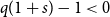 $q(1+s)-1<0$
.
$q(1+s)-1<0$
.
5.3 Results
5.3.1 Main results
Table 2 provides the welfare-maximizing announced CIT rate,
 $\tau^{WM}$
, the growth-maximizing announced rate,
$\tau^{WM}$
, the growth-maximizing announced rate,
 $\tau^{GM}$
, and the growth-maximizing effective CIT rate,
$\tau^{GM}$
, and the growth-maximizing effective CIT rate,
 $\tilde\tau^{GM}$
for the benchmark case. We find that
$\tilde\tau^{GM}$
for the benchmark case. We find that
 $\tau^{WM}=$
0.4025,
$\tau^{WM}=$
0.4025,
 $\tau^{GM}=$
0.3921, and
$\tau^{GM}=$
0.3921, and
 $\tilde{\tau}^{GM}=$
0.3133. The value of the optimal CIT rate, 0.4025, is close to the estimated value of 42% by Aghion et al. (Reference Aghion, Akcigit, Cagé and Kerr2016). As Propositions 4 and 5 indicate,
$\tilde{\tau}^{GM}=$
0.3133. The value of the optimal CIT rate, 0.4025, is close to the estimated value of 42% by Aghion et al. (Reference Aghion, Akcigit, Cagé and Kerr2016). As Propositions 4 and 5 indicate,
 $\tau^{WM}$
,
$\tau^{WM}$
,
 $\tau^{GM}$
, and
$\tau^{GM}$
, and
 $\tilde{\tau}^{GM}$
are all larger than
$\tilde{\tau}^{GM}$
are all larger than
 $\beta(=0.1)$
. Importantly, the difference between
$\beta(=0.1)$
. Importantly, the difference between
 $\tau^{WM}$
and
$\tau^{WM}$
and
 $\beta$
is 0.3025, which is quite large.
$\beta$
is 0.3025, which is quite large.
Table 2. The welfare- and growth-maximizing tax rates and the contributions to
 $\tau^{WM} - \beta$
for the benchmark
$\tau^{WM} - \beta$
for the benchmark
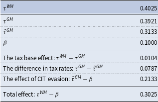
The fifth, sixth, and seventh rows of Table 2 provide a decomposition of the total effect,
 $\tau^{WM}-\beta$
. The effect of CIT evasion,
$\tau^{WM}-\beta$
. The effect of CIT evasion,
 $\tilde{\tau}^{GM}-\beta$
, amounts to 0.2133 and is the largest of the three effects. Thus, the effect of CIT evasion is the primary source of the high optimal CIT rate quantitatively.
$\tilde{\tau}^{GM}-\beta$
, amounts to 0.2133 and is the largest of the three effects. Thus, the effect of CIT evasion is the primary source of the high optimal CIT rate quantitatively.
5.3.2 Robustness
The effect of CIT evasion depends on the markup rate
 $\mu$
(
$\mu$
(
 $=\Gamma(\tau)/\alpha-1$
) because it is related to their market power. Therefore, we calculate the optimal CIT rates for the various markup rates: see Table 3.Footnote 30
$=\Gamma(\tau)/\alpha-1$
) because it is related to their market power. Therefore, we calculate the optimal CIT rates for the various markup rates: see Table 3.Footnote 30
Table 3. The optimal CIT rates for alternative markup rates (benchmark: markup rate
 $=0.20$
)
$=0.20$
)

Around the benchmark value (e.g., the case of markup rate
 $=0.1,...,0.5$
), we find that both
$=0.1,...,0.5$
), we find that both
 $\tau^{GM}$
and
$\tau^{GM}$
and
 $\tau^{WM}$
are much higher than
$\tau^{WM}$
are much higher than
 $\beta$
. In particular, the effect of CIT evasion,
$\beta$
. In particular, the effect of CIT evasion,
 $\tilde{\tau}^{GM}-\beta$
, is significantly large for the alternative markup rates. This indicates that the effect of CIT evasion is the main source of the high optimal CIT rates.
$\tilde{\tau}^{GM}-\beta$
, is significantly large for the alternative markup rates. This indicates that the effect of CIT evasion is the main source of the high optimal CIT rates.
Unsurprisingly, the level of the optimal CIT rate substantially changes according to the output elasticity of public services. However, we find that the impact of tax evasion remains relatively strong for the alternative values of
 $\beta$
, the output elasticity of public services.Footnote 31 In Table 4, we provide the ratio of the welfare-maximizing CIT rate to the output elasticity of public services,
$\beta$
, the output elasticity of public services.Footnote 31 In Table 4, we provide the ratio of the welfare-maximizing CIT rate to the output elasticity of public services,
 $\tau^{WM}/\beta$
. Remember that the criterion in the comparison with the Barro rule is
$\tau^{WM}/\beta$
. Remember that the criterion in the comparison with the Barro rule is
 $\beta$
. Thus, for example, although
$\beta$
. Thus, for example, although
 $\tau^{WM} \approx 0.1$
in the case of
$\tau^{WM} \approx 0.1$
in the case of
 $\beta=0.025$
, we can interpret this rate as a relatively large value. Because the ratios in Table 4 show that the optimal CIT rates are much higher than
$\beta=0.025$
, we can interpret this rate as a relatively large value. Because the ratios in Table 4 show that the optimal CIT rates are much higher than
 $\beta$
, we can confirm the effect of tax evasion on the optimal CIT rate.
$\beta$
, we can confirm the effect of tax evasion on the optimal CIT rate.
Table 4. We provide
 $\tau^{WM}$
, the ratio of
$\tau^{WM}$
, the ratio of
 $\tau^{WM}$
to
$\tau^{WM}$
to
 $\beta$
, and the shares of the effect of CIT evasion in the total effect for alternative output elasticities of public services (benchmark:
$\beta$
, and the shares of the effect of CIT evasion in the total effect for alternative output elasticities of public services (benchmark:
 $\beta=0.10$
)
$\beta=0.10$
)
Next, we calculate the share of the effect of CIT evasion in the total effect,
 $\frac{\tilde{\tau}^{GM}-\beta}{\tau^{WM}-\beta}$
, for the alternative values of
$\frac{\tilde{\tau}^{GM}-\beta}{\tau^{WM}-\beta}$
, for the alternative values of
 $\beta$
. In the benchmark case, the share is 70%. For any other case, the effect of CIT evasion occupies more than half of the total effect. This ensures the robustness of the relative importance of the effect of CIT evasion.
$\beta$
. In the benchmark case, the share is 70%. For any other case, the effect of CIT evasion occupies more than half of the total effect. This ensures the robustness of the relative importance of the effect of CIT evasion.
Table 5. The optimal tax rates in the case of
 $q=0.089$
for the benchmark
$q=0.089$
for the benchmark
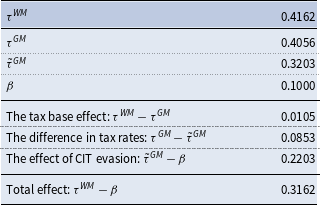
Finally, we conduct a robustness check of the main result with respect to the audit rate q. Figure 1 illustrates the result. Indeed, the level of the optimal CIT rate changes according to q. However, for the various alternative values of q, we can confirm that the effect of CIT evasion is the dominant factor of the high optimal CIT rate relative to the output elasticity of public services.Footnote 32
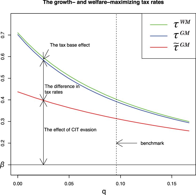
Figure 1. The growth- and welfare-maximizing tax rates (
 $\tau^{WM}$
,
$\tau^{WM}$
,
 $\tau^{GM}$
,
$\tau^{GM}$
,
 $\tilde{\tau}^{GM}$
and contributions to
$\tilde{\tau}^{GM}$
and contributions to
 $\tau^{WM}>\beta$
for alternative values of q).
$\tau^{WM}>\beta$
for alternative values of q).
6. Concluding remarks
This study investigates the optimal CIT in an endogenous growth model with productive public services, incorporating tax evasion by monopolistically competitive producers of intermediate goods.
We show that the growth- and welfare-maximizing CIT rates are higher than the output elasticity of productive public services. Thus, because of tax evasion by firms, the CIT rate should be higher than the output elasticity of public services. This is mainly because CIT evasion mitigates the negative effect of CIT on growth and increases the benefit of raising the CIT rate to provide productive public services. Under plausible parameter values, our numerical exercises show that the effect of CIT evasion is significant and that the optimal level of the CIT rate is much higher than the output elasticity of public services.
Next, we note the limitations of our theoretical framework and discuss directions for future research. First, we assume that the probability of audit (q) and the additional tax rate (s) are exogenous parameters. This is because, in addition to the theoretical simplicity, controlling these parameters would not prevent tax evasion in our framework, owing to actual budgetary constraints and its ineffectiveness as a penalty.Footnote 33 However, because of the budgetary problem faced by tax agencies, there is a trade-off between enlarging the audit system and keeping the tax revenue under reasonable (fiscal and/or legal) constraints. Therefore, it is worthwhile designing a corporate taxation scheme in which the probability of audit and the additional tax rate (q and s in the model) can be chosen.
A further question is how the optimal CIT rates are affected by the presence of international tax competition. This model can be extended to open economies that incorporate tax competition in the locational choice of firms. With such an extension, reducing the CIT rate can have a growth-enhancing effect and play a crucial role in attracting foreign firms. However, a race to bottom with relation to CIT does not occur because it leads to a shortage of public infrastructure that attracts domestic investment (e.g., Dewit et al. (Reference Dewit, Hynes and Leahy2017)). A positive CIT rate can exist in the game. This prediction might align with international negotiations over a minimum CIT rate, to be held in October 2021. Therefore, an empirical analysis is recommended for future studies.
Acknowledgments
We are grateful to Shingo Ishiguro, So Kubota, Kazutoshi Miyazawa, Ryoji Ohdoi, Makoto Saito, Daichi Shirai, Koki Sugawara, Yuta Takahashi, Akira Yakita, and Taiyo Yoshimi for their helpful comments. We also thank the participants of the 2018 Public Economic Theory Conference, Journées LAGV 2018, 2018 Australasian Meeting of Econometric Society, MUETEI workshop at Meisei University, Nagoya Macroeconomic Workshop, Economic Theory and Policy Workshop, the Macro Money Workshop at Hitotsubashi University, and the Economics Seminar at Tokyo International University. We are responsible for any remaining errors.
Appendix
A.1 Proof of lemma
We show that if
 $1-q(1+s)>0$
, the declared profit of the firm i,
$1-q(1+s)>0$
, the declared profit of the firm i,
 $\tilde{\pi}_{i,t}$
, satisfies (12). To do so, we consider two types of dishonest firms: those that do not declare (12), and those that declare (12).
$\tilde{\pi}_{i,t}$
, satisfies (12). To do so, we consider two types of dishonest firms: those that do not declare (12), and those that declare (12).
We begin with a firm of the first type that declares
 $ \tilde{\tilde{\pi}}_{i,t} $
, which is not equal to (12). In this case, this firm is audited with probability one;
$ \tilde{\tilde{\pi}}_{i,t} $
, which is not equal to (12). In this case, this firm is audited with probability one;
 $ \bar{q}=1 $
. Thus, the expected after-tax profit of this firm is given by
$ \bar{q}=1 $
. Thus, the expected after-tax profit of this firm is given by
 \begin{eqnarray} \tilde{\tilde{\pi}}^e_{i,t}=\pi_{i,t}-\tau\tilde{\tilde{\pi}}_{i,t}-1\times(1+s)\tau \left( \pi_{i,t}-\tilde{\tilde{\pi}}_{i,t} \right). \end{eqnarray}
We next consider a dishonest firm that declares (12). This firm is audited with a probability lower than one;
 $ \bar{q} = q \in[0,1)$
, and the expected after-tax profit is given by
$ \bar{q} = q \in[0,1)$
, and the expected after-tax profit is given by
 \begin{equation} \tilde{\pi}^e_{i,t} = \pi_{i,t}-\tau\tilde{\pi}_{i,t}-q(1+s)\tau ( \pi_{i,t}-\tilde{\pi}_{i,t} ). \end{equation}
Suppose
 $ \tilde{\pi}^e_{i,t} < \tilde{\tilde{\pi}}^e_{i,t} $
holds. This implies that a dishonest firm declares
$ \tilde{\pi}^e_{i,t} < \tilde{\tilde{\pi}}^e_{i,t} $
holds. This implies that a dishonest firm declares
 $ \tilde{\tilde{\pi}}_{i,t} $
, which is not equal to (12). Using (A1) and (A2), we rearrange
$ \tilde{\tilde{\pi}}_{i,t} $
, which is not equal to (12). Using (A1) and (A2), we rearrange
 $ \tilde{\pi}^e_{i,t} < \tilde{\tilde{\pi}}^e_{i,t} $
as follows:
$ \tilde{\pi}^e_{i,t} < \tilde{\tilde{\pi}}^e_{i,t} $
as follows:
 \begin{align*} & \ \ \pi_{i,t}-\tau\tilde{\pi}_{i,t}-q(1+s)\tau ( \pi_{i,t}-\tilde{\pi}_{i,t} ) < \pi_{i,t}-\tau\tilde{\tilde{\pi}}_{i,t}-(1+s)\tau \left( \pi_{i,t}-\tilde{\tilde{\pi}}_{i,t} \right), \notag\\ \Leftrightarrow & \ \ (1+s)(1-q) \pi_{i,t} - [1-q(1+s)] \tilde{\pi}_{i,t} < s \tilde{\tilde{\pi}}_{i,t}, \notag\\ \Rightarrow & \ \ (1+s)(1-q) \pi_{i,t} -[1-q(1+s)] \tilde{\pi}_{i,t} < s \pi_{i,t}, \notag\\ \Leftrightarrow & \ \ [1-q(1+s) ] \pi_{i,t} < [1-q(1+s)] \tilde{\pi}_{i,t}.\end{align*}
The third line uses the fact that
 $ \tilde{\tilde{\pi}}_{i,t} \le \pi_{i,t} $
. If
$ \tilde{\tilde{\pi}}_{i,t} \le \pi_{i,t} $
. If
 $ 1-q(1+s)>0 $
, the inequality in the last line indicates that
$ 1-q(1+s)>0 $
, the inequality in the last line indicates that
 $ \pi < \tilde{\pi}_{i,t} $
, which contradicts
$ \pi < \tilde{\pi}_{i,t} $
, which contradicts
 $ \tilde{\tilde{\pi}}_{i,t} \le \pi_{i,t} $
. Thus, dishonest firms declare (12).
$ \tilde{\tilde{\pi}}_{i,t} \le \pi_{i,t} $
. Thus, dishonest firms declare (12).
B. Derivations of the true profit: (15), the expected after-tax operating profit: (16), and the facts on the effective cit rate:
$\tilde{\tau}$
when
$1-q(1+s)>0$


Substituting (14) into (7) yields (15). From
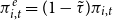 $\pi^e_{i,t}=(1-\tilde{\tau})\pi_{i,t}$
(see (8)) and (15) we obtain (16).
$\pi^e_{i,t}=(1-\tilde{\tau})\pi_{i,t}$
(see (8)) and (15) we obtain (16).
We move onto showing some facts on the effective tax rate when
 $1-q(1+s)>0$
. Here, let us define
$1-q(1+s)>0$
. Here, let us define
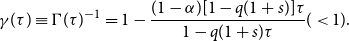 \begin{equation}\gamma(\tau) \equiv \Gamma(\tau)^{-1}=1-\frac{(1-\alpha)[1-q(1+s)]\tau}{1-q(1+s)\tau}(<1). \end{equation}
Substituting (12) (evaluated at
 $p_{i,t}=\tilde{p}_{i,t}$
) and (15) into (9), we have
$p_{i,t}=\tilde{p}_{i,t}$
) and (15) into (9), we have
 \begin{equation}\frac{\tilde{\tau}}{\tau}= [1-q(1+s)]\frac{1-\alpha}{1-\alpha\gamma(\tau)}+q(1+s). \end{equation}
First, we can easily show that
 $ \tilde{\tau}<\tau$
because
$ \tilde{\tau}<\tau$
because
 $[1-q(1+s)]\frac{1-\alpha}{1-\alpha\gamma(\tau)} +q(1+s)-1 = [1-q(1+s)]\left[\frac{1-\alpha}{1-\alpha\gamma(\tau)}-1\right]<0$
, where
$[1-q(1+s)]\frac{1-\alpha}{1-\alpha\gamma(\tau)} +q(1+s)-1 = [1-q(1+s)]\left[\frac{1-\alpha}{1-\alpha\gamma(\tau)}-1\right]<0$
, where
 $\gamma(\tau)<1$
and
$\gamma(\tau)<1$
and
 $1-q(1+s)>0$
.
$1-q(1+s)>0$
.
Second, from the definition of
 $\gamma(\tau)$
and (B2),
$\gamma(\tau)$
and (B2),
 $\displaystyle \lim_{\tau\rightarrow 0}\tilde{\tau}=0$
and
$\displaystyle \lim_{\tau\rightarrow 0}\tilde{\tau}=0$
and
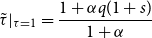 $\displaystyle \tilde{\tau}|_{\tau=1}=\frac{1+\alpha q(1+s)}{1+\alpha}$
and, therefore, we have
$\displaystyle \tilde{\tau}|_{\tau=1}=\frac{1+\alpha q(1+s)}{1+\alpha}$
and, therefore, we have
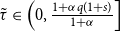 $\tilde{\tau}\in \left(0,\frac{1+\alpha q(1+s)}{1+\alpha} \right]$
.
$\tilde{\tau}\in \left(0,\frac{1+\alpha q(1+s)}{1+\alpha} \right]$
.
C. Relationship between
$\tilde{\tau}$
and
$\tau$


From (B1), we obtain
 \begin{equation}\gamma'(\tau)=-\frac{(1-\alpha)[1-q(1+s)]}{[1-q(1+s)\tau]^2} <0, \end{equation}
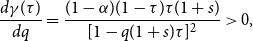 \begin{equation}\frac{d\gamma (\tau)}{dq}=\frac{(1-\alpha)(1-\tau)\tau (1+s)}{[1-q(1+s)\tau]^2}>0,\end{equation}
or both
 $\Gamma'(\tau)>0$
and
$\Gamma'(\tau)>0$
and
 $d\Gamma(\tau)/dq<0$
. From (B2) and (B1), we obtain
$d\Gamma(\tau)/dq<0$
. From (B2) and (B1), we obtain
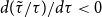 $d(\tilde{\tau}/\tau)/d\tau <0$
. From (B2), (C2), and
$d(\tilde{\tau}/\tau)/d\tau <0$
. From (B2), (C2), and
 $\gamma(\tau)<1$
, we obtain
$\gamma(\tau)<1$
, we obtain
 $d(\tilde{\tau}/\tau)/dq>0$
.
$d(\tilde{\tau}/\tau)/dq>0$
.
Finally, we prove
 $d\tilde{\tau}/d\tau>0$
. From (B2),
$d\tilde{\tau}/d\tau>0$
. From (B2),
 \begin{align}\frac{d\tilde{\tau}}{d\tau}=\frac{[1-q(1+s)](1-\alpha)}{[1-\alpha\gamma(\tau)]^2}\left[1-\alpha\gamma(\tau)+\alpha\tau \gamma'(\tau)\right]+q(1+s) \end{align}
Thus, we have
 $\frac{d\tilde{\tau}}{d\tau}>0$
, if and only if
$\frac{d\tilde{\tau}}{d\tau}>0$
, if and only if
 \begin{equation}1-\alpha\gamma(\tau)+\alpha\tau \gamma'(\tau)>-\frac{[1-\alpha\gamma(\tau)]^2 q(1+s)}{[1-q(1+s)](1-\alpha)} \end{equation}
From
 $\gamma'(\tau)<0$
and
$\gamma'(\tau)<0$
and
 $\gamma''(\tau)<0$
,
$\gamma''(\tau)<0$
,
 $\frac{d}{d\tau}[1-\alpha\gamma(\tau)+\alpha\tau \gamma'(\tau)]=-\alpha\gamma^\prime(\tau)+\alpha\tau\gamma''(\tau)<0$
holds. This indicates that the LHS of (C4) is decreasing in
$\frac{d}{d\tau}[1-\alpha\gamma(\tau)+\alpha\tau \gamma'(\tau)]=-\alpha\gamma^\prime(\tau)+\alpha\tau\gamma''(\tau)<0$
holds. This indicates that the LHS of (C4) is decreasing in
 $\tau$
. Furthermore, the RHS of (C4) is decreasing in
$\tau$
. Furthermore, the RHS of (C4) is decreasing in
 $\tau$
because of
$\tau$
because of
 $ \gamma(\tau)<1 $
and
$ \gamma(\tau)<1 $
and
 $ \gamma^\prime(\tau)<0 $
. Thus,
$ \gamma^\prime(\tau)<0 $
. Thus,
 $\frac{d\tilde{\tau}}{d\tau}>0$
for any
$\frac{d\tilde{\tau}}{d\tau}>0$
for any
 $\tau\in(0,1)$
if the minimum value of the LHS of (C4),
$\tau\in(0,1)$
if the minimum value of the LHS of (C4),
 $1-\alpha\gamma(1)+\alpha\tau \gamma'(1)$
, is larger than the maximum value of the RHS,
$1-\alpha\gamma(1)+\alpha\tau \gamma'(1)$
, is larger than the maximum value of the RHS,
 $-\frac{[1-\alpha\gamma(0)]^2 q(1+s)}{[1-q(1+s)](1-\alpha)}$
. Using
$-\frac{[1-\alpha\gamma(0)]^2 q(1+s)}{[1-q(1+s)](1-\alpha)}$
. Using
 $\gamma(0)=1$
,
$\gamma(0)=1$
,
 $\gamma(1)=\alpha$
and
$\gamma(1)=\alpha$
and
 $\gamma'(1)=-\frac{1-\alpha}{1-q(1+s)}$
, we obtain
$\gamma'(1)=-\frac{1-\alpha}{1-q(1+s)}$
, we obtain
 \begin{equation}1-\alpha\gamma(1)+\alpha\tau \gamma'(1)-\left\{-\frac{[1-\alpha\gamma(0)]^2 q(1+s)}{[1-q(1+s)](1-\alpha)} \right\}=\frac{(1-\alpha)[1-\alpha q(1+s)]}{1-q(1+s)}>0,\end{equation}
and therefore,
 $\frac{d\tilde{\tau}}{d\tau}>0$
for any
$\frac{d\tilde{\tau}}{d\tau}>0$
for any
 $\tau\in(0,1)$
.
$\tau\in(0,1)$
.
D. Derivation of equilibrium conditions
The price level of firm i and j whose productivity is
 $b_i$
and
$b_i$
and
 $b_j$
is
$b_j$
is
 $ p_{i,t} = \frac{\Theta}{\alpha b_i}w_t$
and
$ p_{i,t} = \frac{\Theta}{\alpha b_i}w_t$
and
 $p_{j,t} = \frac{\Theta}{\alpha b_j}w_t$
, where
$p_{j,t} = \frac{\Theta}{\alpha b_j}w_t$
, where
 $\Theta=1(\Gamma(\tilde{\tau}))$
for
$\Theta=1(\Gamma(\tilde{\tau}))$
for
 $1-q(1+s)\leq (>)0$
. Combining these with (3) yields
$1-q(1+s)\leq (>)0$
. Combining these with (3) yields
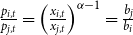 $\frac{p_{i,t}}{p_{j,t}}=\left(\frac{x_{i,t}}{x_{j,t}}\right)^{\alpha-1}=\frac{b_j}{b_i}$
. Thus, we have
$\frac{p_{i,t}}{p_{j,t}}=\left(\frac{x_{i,t}}{x_{j,t}}\right)^{\alpha-1}=\frac{b_j}{b_i}$
. Thus, we have
 $x_{i,t}=\left(\frac{b_j}{b_i}\right)^{\frac{1}{\alpha-1}} x_{j,t} $
. This together with (1), (2), and (3) rewrites
$x_{i,t}=\left(\frac{b_j}{b_i}\right)^{\frac{1}{\alpha-1}} x_{j,t} $
. This together with (1), (2), and (3) rewrites
 $p_{i,t} = \frac{\Theta}{\alpha b_i}w_t$
into
$p_{i,t} = \frac{\Theta}{\alpha b_i}w_t$
into
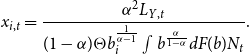 \begin{equation}x_{i,t}=\frac{\alpha^2 L_{Y,t}}{(1-\alpha)\Theta b_i^{\frac{1}{\alpha-1}}\int b^{\frac{\alpha}{1-\alpha}}dF(b)N_t}. \end{equation}
From (22) and (D1), we obtain labor employed in the final good sector as follows:
 \begin{equation}L_{Y,t}=\frac{(1-\alpha)\Theta}{(1-\alpha)\Theta+\alpha^2}L. \end{equation}
Substituting (D2) into (D1) leads to
 \begin{equation}x(p_{i,t})=\left[\frac{\alpha^2}{(1-\alpha)\Theta+\alpha^2}\right]\frac{b_i^{\frac{1}{1-\alpha}}} {\int b^{\frac{\alpha}{1-\alpha}}dF(b)}\frac{L}{N_t}.\end{equation}
From (1) and (3), we obtain
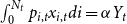 $\int_0^{N_t}p_{i,t}x_{i,t}di=\alpha Y_t$
. Combining
$\int_0^{N_t}p_{i,t}x_{i,t}di=\alpha Y_t$
. Combining
 $\int_0^{N_t}p_{i,t}x_{i,t}di=\alpha Y_t$
with
$\int_0^{N_t}p_{i,t}x_{i,t}di=\alpha Y_t$
with
 $\pi^{e}_{i,t}=(1-\tilde{\tau})\left(1-\alpha \Theta^{-1} \right)p_{i,t}x(p_{i,t})$
, we obtain the total expected after-tax operating profit,
$\pi^{e}_{i,t}=(1-\tilde{\tau})\left(1-\alpha \Theta^{-1} \right)p_{i,t}x(p_{i,t})$
, we obtain the total expected after-tax operating profit,
 $N_t\int \pi^e_{i,t}dF(b) =(1-\tilde{\tau})(1-\alpha \Theta^{-1})\alpha Y_t$
. By combining the total expected after-tax operating profit with (6), we obtain the gross interest rate
$N_t\int \pi^e_{i,t}dF(b) =(1-\tilde{\tau})(1-\alpha \Theta^{-1})\alpha Y_t$
. By combining the total expected after-tax operating profit with (6), we obtain the gross interest rate
 \begin{equation}R_{t-1}=\frac{(1-\tilde{\tau})(1-\alpha\Theta^{-1})\alpha Y_t}{\eta N_t}. \end{equation}
Combining
 $\pi_{i,t}=(1-\alpha\Theta^{-1})p_{i,t}x(p_{i,t})$
with
$\pi_{i,t}=(1-\alpha\Theta^{-1})p_{i,t}x(p_{i,t})$
with
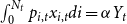 $\int_0^{N_t}p_{i,t}x_{i,t}di=\alpha Y_t$
, the budget constraint of the government (20) is rewritten into
$\int_0^{N_t}p_{i,t}x_{i,t}di=\alpha Y_t$
, the budget constraint of the government (20) is rewritten into
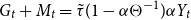 $G_t+M_t=\tilde{\tau}(1-\alpha\Theta^{-1})\alpha Y_t$
. Dividing both sides of the final good market clearing condition,
$G_t+M_t=\tilde{\tau}(1-\alpha\Theta^{-1})\alpha Y_t$
. Dividing both sides of the final good market clearing condition,
 $Y_t =C_t + \eta N_{t+1} +G_t +M_t$
, by
$Y_t =C_t + \eta N_{t+1} +G_t +M_t$
, by
 $N_t$
and using
$N_t$
and using
 $G_t+M_t=\tilde{\tau}(1-\alpha\Theta^{-1})\alpha Y_t$
yield
$G_t+M_t=\tilde{\tau}(1-\alpha\Theta^{-1})\alpha Y_t$
yield
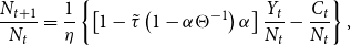 \begin{equation}\frac{N_{t+1}}{N_t}=\frac{1}{\eta}\left\{ \left[1-\tilde{\tau}\left(1-\alpha\Theta^{-1}\right)\alpha\right]\frac{Y_t}{N_t}-\frac{C_t}{N_t}\right\}, \end{equation}
and substituting (D4) into (18), we obtain
 \begin{equation}\frac{C_{t+1}}{C_t}=\left[ \frac{(1-\tilde{\tau})\left(1-\alpha\Theta^{-1} \right) \alpha}{(1+\rho)\eta} \frac{Y_{t+1}}{N_{t+1}} \right]^{1/\sigma}. \end{equation}
Substituting
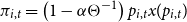 $\pi_{i,t}=\left(1-\alpha \Theta^{-1} \right)p_{i,t}x(p_{i,t})$
into (21) reduces to
$\pi_{i,t}=\left(1-\alpha \Theta^{-1} \right)p_{i,t}x(p_{i,t})$
into (21) reduces to
 $G_t=(1-Q)\tilde{\tau}(1-\alpha\Theta^{-1})\alpha Y_t$
. Combining it with (1), (D2), and (D3), we obtain
$G_t=(1-Q)\tilde{\tau}(1-\alpha\Theta^{-1})\alpha Y_t$
. Combining it with (1), (D2), and (D3), we obtain
 $\frac{Y_t}{N_t}= \Omega(\tilde{\tau})$
. Substituting
$\frac{Y_t}{N_t}= \Omega(\tilde{\tau})$
. Substituting
 $\frac{Y_t}{N_t}= \Omega(\tilde{\tau})$
into (D5) and (D6) and dividing (D6) by (D5) leads to (23).
$\frac{Y_t}{N_t}= \Omega(\tilde{\tau})$
into (D5) and (D6) and dividing (D6) by (D5) leads to (23).
E. Proof of Proposition 3
Let us define the right-hand side (RHS) of (23) as
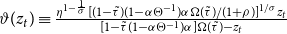 $\vartheta (z_t)\equiv \frac{ \eta^{1-\frac{1}{\sigma}} [(1-\tilde{\tau})(1-\alpha\Theta^{-1})\alpha \Omega(\tilde{\tau})/(1+\rho) ]^{1/\sigma} z_t}{[1-\tilde{\tau}(1-\alpha\Theta^{-1})\alpha]\Omega(\tilde{\tau}) -z_t } $
. Here, note that the denominator of
$\vartheta (z_t)\equiv \frac{ \eta^{1-\frac{1}{\sigma}} [(1-\tilde{\tau})(1-\alpha\Theta^{-1})\alpha \Omega(\tilde{\tau})/(1+\rho) ]^{1/\sigma} z_t}{[1-\tilde{\tau}(1-\alpha\Theta^{-1})\alpha]\Omega(\tilde{\tau}) -z_t } $
. Here, note that the denominator of
 $\vartheta (z_t)$
:
$\vartheta (z_t)$
:
 $[1-\tilde{\tau}(1-\alpha\Theta^{-1})\alpha]\Omega(\tilde{\tau}) -z_t$
must be positive, that is,
$[1-\tilde{\tau}(1-\alpha\Theta^{-1})\alpha]\Omega(\tilde{\tau}) -z_t$
must be positive, that is,
 $z_t< \bar{z}\equiv [1-\tilde{\tau}(1-\alpha\Theta^{-1})\alpha]\Omega(\tilde{\tau})$
, otherwise
$z_t< \bar{z}\equiv [1-\tilde{\tau}(1-\alpha\Theta^{-1})\alpha]\Omega(\tilde{\tau})$
, otherwise
 $N_t$
eventually equals to zero from (D5):
$N_t$
eventually equals to zero from (D5):
 $\frac{N_{t+1}}{N_t}=\frac{1}{\eta}\left\{ \left[1-\tilde{\tau}\left(1-\alpha\Theta^{-1}\right)\alpha\right] \Omega(\tilde{\tau})-z_t \right\}$
. When
$\frac{N_{t+1}}{N_t}=\frac{1}{\eta}\left\{ \left[1-\tilde{\tau}\left(1-\alpha\Theta^{-1}\right)\alpha\right] \Omega(\tilde{\tau})-z_t \right\}$
. When
 $N_t=0$
, both output and consumption equal to zero, which violates the first-order condition of the representative household.
$N_t=0$
, both output and consumption equal to zero, which violates the first-order condition of the representative household.
The properties of
 $\vartheta (z_t)$
for
$\vartheta (z_t)$
for
 $z_t\in[0, \bar{z})$
are as follows:
$z_t\in[0, \bar{z})$
are as follows:
 \begin{align}\vartheta (0)&=0, \lim_{z_t\rightarrow \bar{z}}\vartheta(z_t) =+\infty, \nonumber\\[4pt]\vartheta'(z_t)&= \frac{ \eta^{1-\frac{1}{\sigma}} [(1-\tilde{\tau})(1-\alpha\Theta^{-1})\alpha \Omega(\tilde{\tau})/(1+\rho) ]^{1/\sigma}[1-\tilde{\tau}(1-\alpha\Theta^{-1})\alpha]\Omega(\tilde{\tau}) }{\{[1-\tilde{\tau}(1-\alpha\Theta^{-1})\alpha]\Omega(\tilde{\tau}) -z_t \}^2} >0, \nonumber\\[4pt]\vartheta'(0)&=\frac{ \eta\left[ (1-\tilde{\tau})\left(1-\alpha\Theta^{-1} \right) \alpha(1+\rho)^{-1}\eta^{-1} \Omega(\tilde{\tau}) \right]^{1/\sigma}}{\left[1-\tilde{\tau}\left(1-\alpha\Theta^{-1}\right)\alpha \right]\Omega(\tilde{\tau})}, \lim_{z_t\rightarrow \bar{z}} \vartheta'(z_t)=+\infty\nonumber\\[4pt]\vartheta''(z_t)&= \frac{ 2\eta^{1-\frac{1}{\sigma}} [(1-\tilde{\tau})(1-\alpha\Theta^{-1})\alpha \Omega(\tilde{\tau})/(1+\rho) ]^{1/\sigma}[1-\tilde{\tau}(1-\alpha\Theta^{-1})\alpha]\Omega(\tilde{\tau}) }{\{[1-\tilde{\tau}(1-\alpha\Theta^{-1})\alpha]\Omega(\tilde{\tau}) -z_t \}^3} >0. \end{align}
(E1) indicates that
 $\vartheta(z_t)$
is monotonically increasing and convex function of
$\vartheta(z_t)$
is monotonically increasing and convex function of
 $z_t$
and takes zero when
$z_t$
and takes zero when
 $z_t=0$
.
$z_t=0$
.
Meanwhile, the left-hand side (LHS) of (23) represents
 $45^{\circ}$
line. Thus, we find that a unique steady state
$45^{\circ}$
line. Thus, we find that a unique steady state
 $\hat{z}\in(0, \bar{z})$
, which is unstable exists if and only if
$\hat{z}\in(0, \bar{z})$
, which is unstable exists if and only if
 $\vartheta'(0)<1$
holds. From (D5), (D6) and
$\vartheta'(0)<1$
holds. From (D5), (D6) and
 $Y_t/N_t=\Omega (\tau)$
,
$Y_t/N_t=\Omega (\tau)$
,
 $C_t$
,
$C_t$
,
 $N_t$
, and
$N_t$
, and
 $Y_t$
grow at the same constant rate,
$Y_t$
grow at the same constant rate,
 $C_{t+1}/C_t = N_{t+1}/N_t =Y_{t+1}/Y_t=\hat{g}$
in the steady state.
$C_{t+1}/C_t = N_{t+1}/N_t =Y_{t+1}/Y_t=\hat{g}$
in the steady state.
The rest of this appendix shows that the TVC (19) ensures
 $\vartheta'(0)<1$
. (26) and the asset market clearing condition,
$\vartheta'(0)<1$
. (26) and the asset market clearing condition,
 $W_t=\eta N_{t+1}$
together with the assumption
$W_t=\eta N_{t+1}$
together with the assumption
 $N_0=1$
transform the TVC (19) into
$N_0=1$
transform the TVC (19) into
 $\lim_{t \rightarrow \infty} \frac{\hat{z}^{-\sigma}\hat{g}^{t(1-\sigma)}}{(1+\rho)^t}=0$
. To satisfy the TVC,
$\lim_{t \rightarrow \infty} \frac{\hat{z}^{-\sigma}\hat{g}^{t(1-\sigma)}}{(1+\rho)^t}=0$
. To satisfy the TVC,
 $1>(1+\rho)^{-1}\hat g^{1-\sigma}$
must holds.
$1>(1+\rho)^{-1}\hat g^{1-\sigma}$
must holds.
 $1>(1+\rho)^{-1}\hat g^{1-\sigma}$
and (26) together with
$1>(1+\rho)^{-1}\hat g^{1-\sigma}$
and (26) together with
 $\frac{(1-\tilde{\tau})(1-\alpha\Theta^{-1})\alpha}{1-\tilde{\tau}(1-\alpha\Theta^{-1})\alpha}<1$
lead to
$\frac{(1-\tilde{\tau})(1-\alpha\Theta^{-1})\alpha}{1-\tilde{\tau}(1-\alpha\Theta^{-1})\alpha}<1$
lead to
 $\vartheta'(0)<1$
.
$\vartheta'(0)<1$
.
F. Proof of Proposition 4
F.1 Proof of 1
In this case, since each firm does not evade CIT,
 $\Theta=1$
and
$\Theta=1$
and
 $\tilde\tau=\tau$
. Then, by (24) and (26), we obtain
$\tilde\tau=\tau$
. Then, by (24) and (26), we obtain
 $\tilde{\tau}^{GM}=\tau^{GM}=\alpha$
immediately.
$\tilde{\tau}^{GM}=\tau^{GM}=\alpha$
immediately.
F.2 Proof of 2
In the beginning, note that the decision of optimal announced CIT rate is equivalent to that of the optimal effective CIT rate. This is because
 $\tilde{\tau}$
is the function of
$\tilde{\tau}$
is the function of
 $\tau$
from (B2), and
$\tau$
from (B2), and
 $\tilde{\tau}$
is strictly increasing in
$\tilde{\tau}$
is strictly increasing in
 $\tau$
,
$\tau$
,
 $d\tilde{\tau}/d \tau >0$
, for any
$d\tilde{\tau}/d \tau >0$
, for any
 $\tau\in(0,1)$
, as shown in Appendix C.
$\tau\in(0,1)$
, as shown in Appendix C.
Because the growth rate converges to 0 as
 $\tau$
goes to 0 by the construction of the model, the growth rate is maximized at 1 or some interior point in (0, 1).
$\tau$
goes to 0 by the construction of the model, the growth rate is maximized at 1 or some interior point in (0, 1).
First, we prove that the growth-maximizing effective CIT is higher than
 $\alpha$
when it is an interior point in (0, 1). From the definition of
$\alpha$
when it is an interior point in (0, 1). From the definition of
 $\Omega(\tilde{\tau})$
and (D6), growth maximization with respect to
$\Omega(\tilde{\tau})$
and (D6), growth maximization with respect to
 $\tilde{\tau}$
is equivalent to
$\tilde{\tau}$
is equivalent to
 $\displaystyle\max_{\tilde{\tau}}f(\tilde{\tau})=\ln(1-\tilde{\tau})\tilde{\tau}^{\frac{\alpha}{1-\alpha}} [1-\alpha\gamma(\tau)]^{\frac{1}{1-\alpha}}\gamma(\tau)^{\frac{\alpha}{1-\alpha}} [{1-\alpha+\alpha^2 \gamma(\tau)} ]^{-\frac{1}{1-\alpha}}$
, subject to (B2):
$\displaystyle\max_{\tilde{\tau}}f(\tilde{\tau})=\ln(1-\tilde{\tau})\tilde{\tau}^{\frac{\alpha}{1-\alpha}} [1-\alpha\gamma(\tau)]^{\frac{1}{1-\alpha}}\gamma(\tau)^{\frac{\alpha}{1-\alpha}} [{1-\alpha+\alpha^2 \gamma(\tau)} ]^{-\frac{1}{1-\alpha}}$
, subject to (B2):
 $\frac{\tilde{\tau}}{\tau}= [1-q(1+s)]\frac{1-\alpha}{1-\alpha\gamma(\tau)}+q(1+s)$
. The first derivative of
$\frac{\tilde{\tau}}{\tau}= [1-q(1+s)]\frac{1-\alpha}{1-\alpha\gamma(\tau)}+q(1+s)$
. The first derivative of
 $f(\tilde{\tau})$
is
$f(\tilde{\tau})$
is
 \begin{equation}f'(\tilde{\tau})=\bigg[\underbrace{-\frac{1}{1-\tilde{\tau}} + \frac{\alpha}{1-\alpha}\frac{1}{\tilde{\tau}}}_{\equiv \Psi_1(\tilde{\tau})} \bigg]+\frac{\alpha}{1-\alpha}\frac{d\tau}{d\tilde{\tau}}\gamma '(\tau)\bigg[\underbrace{\frac{1}{\gamma(\tau)}-\frac{1}{1-\alpha \gamma (\tau)} -\frac{\alpha}{1-\alpha+\alpha^2 \gamma(\tau)}}_{\equiv \Psi_2(\tau)}\bigg]. \end{equation}
It is obvious that
 $\Psi_1(\tilde{\tau})=-\frac{1}{1-\tilde{\tau}}+\frac{\alpha}{1-\alpha}\frac{1}{\tau}=\frac{\alpha-\tilde{\tau}}{(1-\tilde{\tau})(1-\alpha)\tilde{\tau}}\geq0$
for
$\Psi_1(\tilde{\tau})=-\frac{1}{1-\tilde{\tau}}+\frac{\alpha}{1-\alpha}\frac{1}{\tau}=\frac{\alpha-\tilde{\tau}}{(1-\tilde{\tau})(1-\alpha)\tilde{\tau}}\geq0$
for
 $\tilde{\tau}\leq\alpha$
. Next, we show that the sign of
$\tilde{\tau}\leq\alpha$
. Next, we show that the sign of
 $\Psi_2(\tau)$
is negative for
$\Psi_2(\tau)$
is negative for
 $\tilde{\tau}\leq\alpha$
.
$\tilde{\tau}\leq\alpha$
.
 \begin{align}\mbox{sign}\Psi_2(\tau)&= [1-\alpha\gamma(\tau)][1-\alpha+\alpha^2 \gamma(\tau)]-\gamma(\tau)[1-\alpha+\alpha^2 \gamma(\tau)]-\alpha\gamma(\tau)[1-\alpha\gamma(\tau)]\nonumber\\&=-\alpha^3\gamma(\tau)^2-(1-\alpha)[(1+2\alpha)\gamma(\tau)-1] \end{align}
Here,
 $\mbox{sign}\Psi_2(\tau)<0$
for
$\mbox{sign}\Psi_2(\tau)<0$
for
 $\gamma(\tau)>\frac{1}{1+2\alpha}$
. Furthermore, (B1) and (B2) indicate that
$\gamma(\tau)>\frac{1}{1+2\alpha}$
. Furthermore, (B1) and (B2) indicate that
 $\gamma(\tau)$
is increasing in
$\gamma(\tau)$
is increasing in
 $q(1+s)$
and when
$q(1+s)$
and when
 $q(1+s)=0$
,
$q(1+s)=0$
,
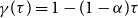 $\gamma(\tau)=1-(1-\alpha)\tau$
,
$\gamma(\tau)=1-(1-\alpha)\tau$
,
 $\tau=\frac{\tilde{\tau}}{1-\alpha\tilde{\tau}}$
and
$\tau=\frac{\tilde{\tau}}{1-\alpha\tilde{\tau}}$
and
 $\gamma(\frac{\tilde{\tau}}{1-\alpha\tilde{\tau}})=\frac{1-\tilde{\tau}}{1-\alpha\tilde{\tau}}$
hold. From
$\gamma(\frac{\tilde{\tau}}{1-\alpha\tilde{\tau}})=\frac{1-\tilde{\tau}}{1-\alpha\tilde{\tau}}$
hold. From
 $\frac{1-\tilde{\tau}}{1-\alpha\tilde{\tau}}-\frac{1}{1+2\alpha}=\frac{\alpha-\tilde{\tau}+\alpha(1-\tilde{\tau})}{(1-\alpha\tilde{\tau})(1+2\alpha)}>0$
, we obtain
$\frac{1-\tilde{\tau}}{1-\alpha\tilde{\tau}}-\frac{1}{1+2\alpha}=\frac{\alpha-\tilde{\tau}+\alpha(1-\tilde{\tau})}{(1-\alpha\tilde{\tau})(1+2\alpha)}>0$
, we obtain
 $\gamma(\frac{\tilde{\tau}}{1-\alpha\tilde{\tau}})=\frac{1-\tilde{\tau}}{1-\alpha\tilde{\tau}}>\frac{1}{1+2\alpha}$
for
$\gamma(\frac{\tilde{\tau}}{1-\alpha\tilde{\tau}})=\frac{1-\tilde{\tau}}{1-\alpha\tilde{\tau}}>\frac{1}{1+2\alpha}$
for
 $\tilde{\tau}\leq\alpha$
. Thus,
$\tilde{\tau}\leq\alpha$
. Thus,
 $\mbox{sign}\Psi_2(\tau)<0$
for
$\mbox{sign}\Psi_2(\tau)<0$
for
 $\tilde{\tau}\leq\alpha$
. Combining
$\tilde{\tau}\leq\alpha$
. Combining
 $\Psi_1(\tilde{\tau})\geq0$
and
$\Psi_1(\tilde{\tau})\geq0$
and
 $\Psi_2(\tilde{\tau})<0$
for
$\Psi_2(\tilde{\tau})<0$
for
 $\tilde{\tau}\leq\alpha$
with
$\tilde{\tau}\leq\alpha$
with
 $\gamma'(\tau)<0$
((B2)) and
$\gamma'(\tau)<0$
((B2)) and
 $\frac{d\tilde{\tau}}{d\tau}>0$
, we obtain
$\frac{d\tilde{\tau}}{d\tau}>0$
, we obtain
 $f'(\tilde{\tau})>0$
for
$f'(\tilde{\tau})>0$
for
 $\tilde{\tau}\le\alpha$
. From the discussion so far, we find that
$\tilde{\tau}\le\alpha$
. From the discussion so far, we find that
 $\tilde{\tau}^{GM}>\alpha$
holds.
$\tilde{\tau}^{GM}>\alpha$
holds.
Next, we consider the case of the corner solution of growth-maximization:
 $\tau^{GM}=1$
. Assuming
$\tau^{GM}=1$
. Assuming
 $q(1+s)>\frac{\alpha(1+\alpha)-1}{\alpha}$
additionally, we ensure that
$q(1+s)>\frac{\alpha(1+\alpha)-1}{\alpha}$
additionally, we ensure that
 $\tilde{\tau}^{GM}>\alpha$
because
$\tilde{\tau}^{GM}>\alpha$
because
 $\tilde{\tau}|_{\tau=1}=\frac{1+\alpha q(1+s)}{1+\alpha}$
.Footnote 34
$\tilde{\tau}|_{\tau=1}=\frac{1+\alpha q(1+s)}{1+\alpha}$
.Footnote 34
G. Proof and intuition of Proposition 5
(i) PROOF OF 1
The maximization condition of social welfare is
 $\frac{\partial U}{\partial \tau}=0$
. By (29), this is equivalent to
$\frac{\partial U}{\partial \tau}=0$
. By (29), this is equivalent to
 \begin{align}\big[1-(1+\rho)^{-1}\hat{g}^{1-\sigma}\big]\frac{\partial \hat{z}}{\partial \tau} + (1+\rho)^{-1}\hat{z} \hat{g}^{-\sigma}\frac{\partial \hat{g}}{\partial \tau} = 0. \end{align}
From (25) and (26), with
 $\Theta=1$
, we obtain
$\Theta=1$
, we obtain
 $\hat{z}=\frac{1-\alpha(1-\alpha)\tau}{\eta^{-1}(1+\rho)^{-1}\alpha(1-\alpha)(1-\tau)} \hat g^{\sigma} - \eta\hat g.$
Differentiating it with respect to
$\hat{z}=\frac{1-\alpha(1-\alpha)\tau}{\eta^{-1}(1+\rho)^{-1}\alpha(1-\alpha)(1-\tau)} \hat g^{\sigma} - \eta\hat g.$
Differentiating it with respect to
 $\tau$
yields
$\tau$
yields
 $\frac{\partial \hat z}{\partial \tau} = \frac{\eta (1+\rho)}{\alpha(1-\alpha)}\bigg[\frac{1-\alpha(1-\alpha)}{(1-\tau)^2}\hat{g}^\sigma + \frac{1-\alpha(1-\alpha)\tau}{1-\tau}\sigma \hat{g}^{\sigma-1}\frac{\partial \hat{g}}{\partial \tau}\bigg] - \eta \frac{\partial \hat{g}}{\partial \tau}.$
Substituting it into (G1) and rearranging it using
$\frac{\partial \hat z}{\partial \tau} = \frac{\eta (1+\rho)}{\alpha(1-\alpha)}\bigg[\frac{1-\alpha(1-\alpha)}{(1-\tau)^2}\hat{g}^\sigma + \frac{1-\alpha(1-\alpha)\tau}{1-\tau}\sigma \hat{g}^{\sigma-1}\frac{\partial \hat{g}}{\partial \tau}\bigg] - \eta \frac{\partial \hat{g}}{\partial \tau}.$
Substituting it into (G1) and rearranging it using
 $\hat{z}=\frac{1-\alpha(1-\alpha)\tau}{\eta^{-1}(1+\rho)^{-1}\alpha(1-\alpha)(1-\tau)} \hat g^{\sigma} - \eta\hat g$
, we have
$\hat{z}=\frac{1-\alpha(1-\alpha)\tau}{\eta^{-1}(1+\rho)^{-1}\alpha(1-\alpha)(1-\tau)} \hat g^{\sigma} - \eta\hat g$
, we have
 \begin{align}\frac{\partial \hat{g}}{\partial \tau} = -\frac{\big[1-(1+\rho)^{-1}\hat{g}^{1-\sigma}\big]\frac{(1+\rho)[1-\alpha(1-\alpha)]}{\alpha(1-\alpha)(1-\tau)^2}\hat g^\sigma}{K}, \end{align}
where
 $K = \left[1-(1+\rho)^{-1}\hat{g}^{1-\sigma}\right]\frac{(1+\rho)[1-\alpha(1-\alpha)\tau]}{\alpha(1-\alpha)(1-\tau)}\sigma\hat{g}^{\sigma-1} + \frac{1-\alpha(1-\alpha)}{\alpha(1-\alpha)(1-\tau)} >0$
. Therefore, by (G2), we find that
$K = \left[1-(1+\rho)^{-1}\hat{g}^{1-\sigma}\right]\frac{(1+\rho)[1-\alpha(1-\alpha)\tau]}{\alpha(1-\alpha)(1-\tau)}\sigma\hat{g}^{\sigma-1} + \frac{1-\alpha(1-\alpha)}{\alpha(1-\alpha)(1-\tau)} >0$
. Therefore, by (G2), we find that
 $\frac{\partial \hat g}{\partial \tau}|_{\tau=\tau^{WM}}<0$
. This implies
$\frac{\partial \hat g}{\partial \tau}|_{\tau=\tau^{WM}}<0$
. This implies
 $\tau^{GM}<\tau^{WM}$
because
$\tau^{GM}<\tau^{WM}$
because
 $\hat g$
is a single-peaked function of
$\hat g$
is a single-peaked function of
 $\tau$
(see (26) and the definition of
$\tau$
(see (26) and the definition of
 $\Omega(\tilde{\tau})$
with
$\Omega(\tilde{\tau})$
with
 $\Theta=1$
).
$\Theta=1$
).
(ii) PROOF OF 2
Since
 $\mbox{sign}\big\{\frac{d U}{d\tau}|_{\tau=\tau^{GM}}\big\}=\mbox{sign}\big\{\frac{\partial \hat z}{\partial \tau}|_{\tau=\tau^{GM}}\big\}$
, we show
$\mbox{sign}\big\{\frac{d U}{d\tau}|_{\tau=\tau^{GM}}\big\}=\mbox{sign}\big\{\frac{\partial \hat z}{\partial \tau}|_{\tau=\tau^{GM}}\big\}$
, we show
 $\frac{\partial \hat z}{\partial \tau}|_{\tau=\tau^{GM}}>0$
for
$\frac{\partial \hat z}{\partial \tau}|_{\tau=\tau^{GM}}>0$
for
 $q=0$
. From (26) and (25), with
$q=0$
. From (26) and (25), with
 $\Theta=\Gamma(\tau)=\gamma(\tau)^{-1}$
, we obtain
$\Theta=\Gamma(\tau)=\gamma(\tau)^{-1}$
, we obtain
 $\hat{z}=\frac{1-\alpha\left[1-\alpha \gamma(\tau)\right]\tilde \tau}{\eta^{-1}(1+\rho)^{-1}(1-\tilde \tau)\left[1-\alpha \gamma(\tau)\right]\alpha}\hat g^\sigma-\eta \hat g,$
Differentiating it with respect to
$\hat{z}=\frac{1-\alpha\left[1-\alpha \gamma(\tau)\right]\tilde \tau}{\eta^{-1}(1+\rho)^{-1}(1-\tilde \tau)\left[1-\alpha \gamma(\tau)\right]\alpha}\hat g^\sigma-\eta \hat g,$
Differentiating it with respect to
 $\tau$
, we obtain
$\tau$
, we obtain
 \begin{equation}\frac{\partial \hat{z}}{\partial \tau}\bigg|_{\tau=\tau^{GM}} = \hat g^{\sigma}\frac{(1-\alpha\gamma(\tau))\left[1-\alpha(1-\alpha\gamma(\tau))\right]\frac{d\tilde\tau}{d\tau}+\alpha(1-\tilde\tau)\gamma'(\tau)}{\eta^{-1}(1+\rho)^{-1}\alpha\left[(1-\alpha\gamma(\tau))(1-\tilde \tau)\right]^2} \end{equation}
Here, let us define the numerator of (G3) as J. Through simple algebra, we have
 $\gamma(\tau) = 1-(1-\alpha)\tau$
and
$\gamma(\tau) = 1-(1-\alpha)\tau$
and
 $\tilde\tau = \big[\frac{1-\alpha}{1-\alpha\gamma(\tau)}\big]\tau$
. Hence, utilizing these, we have
$\tilde\tau = \big[\frac{1-\alpha}{1-\alpha\gamma(\tau)}\big]\tau$
. Hence, utilizing these, we have
 \begin{align}J = \frac{\big[1-\alpha(1-\alpha\gamma)\big](1-\alpha)^3}{(1-\alpha\gamma(\tau))\big[1-\alpha(1-\alpha)(1-\alpha\tau)\big]}\big[1-\alpha+\alpha(1+\alpha)\tau\big]. \end{align}
Equation (G4) ensures that
 $J>0$
for any
$J>0$
for any
 $\tau\in{(0,1)}$
. This completes the proof.
$\tau\in{(0,1)}$
. This completes the proof.
(iii) INTUITION OF Proposition 5
For an intuitive interpretation, we focus on the marginal effect of raising the tax rate on the growth-maximizing rate,
 $\tau^{GM}$
. By (29), the lifetime utility,
$\tau^{GM}$
. By (29), the lifetime utility,
 $U_0$
, depends on the long-run growth rate,
$U_0$
, depends on the long-run growth rate,
 $\hat g$
, and the initial consumption,
$\hat g$
, and the initial consumption,
 $\hat z$
. At
$\hat z$
. At
 $\tau=\tau^{GM}$
, the marginal effect of raising
$\tau=\tau^{GM}$
, the marginal effect of raising
 $\tau$
on
$\tau$
on
 $\hat g$
disappears. Then, the CIT rate affects welfare only through the effect on initial consumption:
$\hat g$
disappears. Then, the CIT rate affects welfare only through the effect on initial consumption:
 $\mbox{sign}\left\{\frac{d U}{d \tau}|_{\tau=\tau^{GM}}\right\}=\mbox{sign}\left\{\frac{\partial \hat z}{\partial \tau}|_{\tau=\tau^{GM}}\right\}$
. Note that by (25) and (D4) in Appendix D, the initial consumption is decomposed into
$\mbox{sign}\left\{\frac{d U}{d \tau}|_{\tau=\tau^{GM}}\right\}=\mbox{sign}\left\{\frac{\partial \hat z}{\partial \tau}|_{\tau=\tau^{GM}}\right\}$
. Note that by (25) and (D4) in Appendix D, the initial consumption is decomposed into
 \begin{equation*}\hat{z}=\underbrace{\left[1-\tilde{\tau}\left(1-\alpha\Theta^{-1}\right)\alpha \right]\Omega(\tilde{\tau})}_{\mbox{disposable income}} - \eta\big[ \underbrace{(1-\tilde{\tau})\left(1-\alpha\Theta^{-1} \right) \alpha(1+\rho)^{-1}\eta^{-1} \Omega(\tilde{\tau})}_{=R/(1+\rho)}\big]^{1/\sigma}.\end{equation*}
Because the second term depends on the interest rate, this is a Slutsky decomposition of the initial consumption. Since the interest rate is also maximized at
 $\tau=\tau^{GM}$
, the marginal effect on the second term disappears here. Consequently, the marginal effect of raising
$\tau=\tau^{GM}$
, the marginal effect on the second term disappears here. Consequently, the marginal effect of raising
 $\tau$
on
$\tau$
on
 $\hat{z}$
at
$\hat{z}$
at
 $\tau=\tau^{GM}$
equals that on the disposable income of household.
$\tau=\tau^{GM}$
equals that on the disposable income of household.
The disposable income of a household increases by raising
 $\tau$
from
$\tau$
from
 $\tau^{GM}$
marginally. Thus,
$\tau^{GM}$
marginally. Thus,
 $\tau^{GM}<\tau^{WM}$
. Raising
$\tau^{GM}<\tau^{WM}$
. Raising
 $\tau$
increases before tax income
$\tau$
increases before tax income
 $\Omega(\tilde{\tau})$
. While
$\Omega(\tilde{\tau})$
. While
 $\Omega(\tilde{\tau})$
includes both labor and asset income, CIT is imposed only on the source of asset income, that is, the firms’ profits. Thus, the disposable income of a household increases as a whole. It suggests that the break in the coincidence of growth- and welfare-maximization tax rates is because the tax base is CIT.Footnote 35
$\Omega(\tilde{\tau})$
includes both labor and asset income, CIT is imposed only on the source of asset income, that is, the firms’ profits. Thus, the disposable income of a household increases as a whole. It suggests that the break in the coincidence of growth- and welfare-maximization tax rates is because the tax base is CIT.Footnote 35
H. Proof of remark
We prove the counterpart of Proposition 4 in the Remark by modifying Appendix F as follows.
Under the production technology of the final goods, (30) and (31), the wage rate (2) and the price of intermediate goods (3) are rewritten as
 \begin{align}w_t=(1-\alpha)L_{Y,t}^{-\alpha} \int_0^{N_t} (a(G_t, N_t) x_{i,t})^\alpha di=(1-\alpha)\frac{Y_t}{L_{Y,t}} \end{align}
and
 \begin{equation}p_{i,t} =\alpha A L^{1-\alpha}_{Y,t}a(G_t,N_t)^{\alpha}x^{\alpha-1}_{i,t}, \end{equation}
respectively. These two equations yield the demand function for the product of firm i:
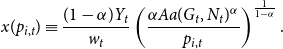 \begin{equation}x(p_{i,t}) \equiv\frac{(1-\alpha)Y_t}{w_t}\left(\frac{\alpha A a(G_t, N_t)^\alpha}{p_{i,t}}\right)^{\frac{1}{1-\alpha}}. \end{equation}
Because the forms of true profit, (7), declared profit, (12), and the effective CIT rate, (9), remain unchanged, we confirm that
 $\frac{\partial \pi_{i,t}}{\partial p_{i,t}}=-\alpha x(p_{i,t}) \left[\frac{p_{i,t}-w_t/(\alpha b_i)}{(1-\alpha)p_{i,t}} \right]$
and
$\frac{\partial \pi_{i,t}}{\partial p_{i,t}}=-\alpha x(p_{i,t}) \left[\frac{p_{i,t}-w_t/(\alpha b_i)}{(1-\alpha)p_{i,t}} \right]$
and
 $\Lambda'(p_{i,t})=-\alpha x(p_{i,t})$
also hold under (H3). Therefore, maximizing the expected after-tax operating profit of firm i, (8), yields the same results as those given in Proposition 2.
$\Lambda'(p_{i,t})=-\alpha x(p_{i,t})$
also hold under (H3). Therefore, maximizing the expected after-tax operating profit of firm i, (8), yields the same results as those given in Proposition 2.
We obtain the equilibrium conditions ((D1), (D2), (D3), (D4) (D5), and (D6)) using the procedure given in Appendix D. To derive these equilibrium conditions, we use the (i) production of the final goods ((30) and (31)), (ii) wage rate (H1), (iii) demand function for the intermediate product (H3), (iv) free-entry condition (6), (v) Euler equation (18), (vi) government’s budget constraints ((20) and (21)), (vii) labor, asset, and final goods market clearing conditions ((22),
 $W_t=\eta N_{t+1}$
, and
$W_t=\eta N_{t+1}$
, and
 $Y_t =C_t +\eta N_{t+1}+G_t+M_t$
), and (viii) results of Proposition 2. Consequently, the dynamic system of the economy is characterized by the same form of difference equation as that in (23). Note that the only difference between the baseline and the extended model is therefore given in (24).
$Y_t =C_t +\eta N_{t+1}+G_t+M_t$
), and (viii) results of Proposition 2. Consequently, the dynamic system of the economy is characterized by the same form of difference equation as that in (23). Note that the only difference between the baseline and the extended model is therefore given in (24).
 $Y_t/N_t (=Y_{t+1}/N_{t+1})$
changes to
$Y_t/N_t (=Y_{t+1}/N_{t+1})$
changes to
 \begin{align}\hat{\Omega}(\tilde{\tau})\equiv&A^{\frac{1}{1-\beta}}\left[(1-Q)\tilde{\tau}\left(1-\alpha \Theta^{-1} \right)\alpha \right]^{\frac{\beta}{1-\beta}} [(1-\alpha)\Theta ]^{\frac{1-\alpha}{1-\beta}}\alpha^{\frac{2\alpha}{1-\beta}}\left[\frac{L}{(1-\alpha)\Theta+\alpha^2}\right]^{\frac{1}{1-\beta}}\nonumber\\&\times \left[\int b^{\frac{\alpha}{1-\alpha}} dF(b)\right]^{\frac{1-\alpha}{1-\beta}}.\end{align}
The unique steady-state value of
 $z_t$
in (25) and economic growth rate
$z_t$
in (25) and economic growth rate
 $\hat{g}$
in (26) are modified by replacing
$\hat{g}$
in (26) are modified by replacing
 $\Omega (\tilde{\tau})$
with
$\Omega (\tilde{\tau})$
with
 $\hat{\Omega}(\tilde{\tau})$
.
$\hat{\Omega}(\tilde{\tau})$
.
From the modified
 $\hat{g}$
and (H4), we have
$\hat{g}$
and (H4), we have
 $\tilde{\tau}^{GM}= \mbox{argmax}\, (1-\tilde{\tau})\tilde{\tau}^{\frac{\beta}{1-\beta}} (1-\alpha\Theta^{-1})^{\frac{1}{1-\beta}}\Theta^{\frac{1-\alpha}{1-\beta}}\left(\frac{\Theta^{-1}}{1-\alpha+\alpha^2 \Theta^{-1}} \right)^{\frac{1}{1-\beta}}$
. (F1) changes as follows:
$\tilde{\tau}^{GM}= \mbox{argmax}\, (1-\tilde{\tau})\tilde{\tau}^{\frac{\beta}{1-\beta}} (1-\alpha\Theta^{-1})^{\frac{1}{1-\beta}}\Theta^{\frac{1-\alpha}{1-\beta}}\left(\frac{\Theta^{-1}}{1-\alpha+\alpha^2 \Theta^{-1}} \right)^{\frac{1}{1-\beta}}$
. (F1) changes as follows:
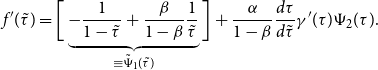 \begin{equation}f'(\tilde{\tau})=\bigg[\underbrace{-\frac{1}{1-\tilde{\tau}} + \frac{\beta}{1-\beta}\frac{1}{\tilde{\tau}}}_{\equiv \tilde{\Psi}_1(\tilde{\tau})} \bigg]+\frac{\alpha}{1-\beta}\frac{d\tau}{d\tilde{\tau}}\gamma '(\tau)\Psi_2(\tau).\end{equation}
Immediately, we have
 $\tilde{\Psi}_1=\frac{\beta-\tilde{\tau}}{(1-\tilde{\tau})(1-\alpha)\tilde{\tau}}\geq 0$
, for
$\tilde{\Psi}_1=\frac{\beta-\tilde{\tau}}{(1-\tilde{\tau})(1-\alpha)\tilde{\tau}}\geq 0$
, for
 $\tilde{\tau}\leq \beta$
. As in Appendix F,
$\tilde{\tau}\leq \beta$
. As in Appendix F,
 $\mbox{sign}\,\Psi_2(\tau)<0$
for
$\mbox{sign}\,\Psi_2(\tau)<0$
for
 $\tilde{\tau}\leq \beta$
, because
$\tilde{\tau}\leq \beta$
, because
 $\beta < \alpha$
. This indicates that
$\beta < \alpha$
. This indicates that
 $\tilde{\tau}^{GM} \ge \beta$
for the interior solution. In addition, we discuss the corner solution (
$\tilde{\tau}^{GM} \ge \beta$
for the interior solution. In addition, we discuss the corner solution (
 $\tau^{GM}=1$
) in the same way as in Appendix F.Footnote 36
$\tau^{GM}=1$
) in the same way as in Appendix F.Footnote 36
The counterpart of Proposition 5 is proved in the same way as Proposition 5. This is because our calculations in Appendix G do not depend on the expression of the growth rate,
 $\hat g$
, which is the unique difference between the baseline and extended model.Footnote 37 Immediately, it has the same property with respect to
$\hat g$
, which is the unique difference between the baseline and extended model.Footnote 37 Immediately, it has the same property with respect to
 $\tau$
as the growth rate in the baseline model. As such, the calculations in Appendix G can be applied to the extended model.
$\tau$
as the growth rate in the baseline model. As such, the calculations in Appendix G can be applied to the extended model.
I. Details of calibration
We seek to obtain quantitative implications for tax evasion in OECD countries.
-
The distribution of productivity is set in such a way that the distribution of firm size is set to the Pareto distribution, which is estimated by Axtell (Reference Axtell2001). By (D1) and (D2), letting
$N_0 = 1$
, we have
where
\begin{align*}\frac{x_i}{b_i} = \underbrace{\bigg[\frac{\alpha^2}{(1-\alpha)\Gamma(\tau)+\alpha^2}\bigg]\frac{L}{\int b^{\frac{\alpha}{1-\alpha}}dF(b)}}_{\equiv B}b_i^{\frac{\alpha}{1-\alpha}},\end{align*}
$\Gamma(\tau)=\frac{1-q(1+s)\tau}{1-q(1+s)\tau-(1-\alpha)\big[1-q(1+s)\big]\tau}$
. This is the size of intermediate good firms. To make its distribution a Pareto distribution, we set the distribution of
$b^{\frac{\alpha}{1-\alpha}}$
to Pareto distribution with scale parameter
$\phi>0$
and shape parameter
$\psi>1$
. Then, letting
$\mbox{SCALE}=B\phi$
, because
$\int b^{\frac{\alpha}{1-\alpha}}dF(b)=\frac{\psi-1}{\psi}\phi$
in B, the distribution of firm size is the Pareto distribution with scale parameter
(I1)and shape parameter
\begin{align}\mbox{SCALE} = \frac{\alpha^2}{(1-\alpha)\Gamma(\tau)+\alpha^2}\frac{\psi-1}{\psi}L, \end{align}
$\psi$
. Since the shape parameter is the most important factor of firm distribution, we set
$\psi = 1.059$
according to the estimate in Axtell (Reference Axtell2001), which uses US data.
-
Next, we control the markup rate of intermediate good firms. Letting the markup rate be
$\mu$
, by (14),
(I2)As the benchmark value of
\begin{align}\frac{\Gamma(\tau)}{\alpha}=1+\mu. \end{align}
$\mu$
, we adopt
$0.2$
, a usual value of the macroeconomic model with imperfect competition.Footnote 38
-
To determine the value of the remaining parameters, we set the benchmark value of
$\tau, q$
, and s exogenously, as shown in Table 1. For their source, see Table 1 and the text. -
There are four undetermined parameters for (I1) and (I2),
$\alpha, L, \mbox{SCALE}$
, and
$\phi$
. Here, we put
$L=\phi=1$
and determine
$\alpha$
and
$\mbox{SCALE}$
by (I1) and (I2). Note that productivity b follows the Pareto distribution with scale parameter
$\phi^{\frac{\alpha}{1-\alpha}}$
and shape parameter
$\frac{1-\alpha}{\alpha}\psi$
, since we assume
$b^{\frac{\alpha}{1-\alpha}}$
follows the Pareto distribution with scale parameter
$\phi$
and shape parameter
$\psi$
. Because the scale of productivity may be arbitrarily fixed whenever the distribution of firm size is properly controlled, we set
$\phi=1$
. We simply normalize
$L=1$
. Since the number of the intermediate good firms is a continuum, the minimum of firm size among them does not have to correspond to the minimal number of employees in actual data (and only the shape of the distribution, the curvature of the density function, matters). Thus, we do not care about the magnitude of parameter
$\mbox{SCALE}$
, which is determined by (I1) for given
$\alpha$
and the other parameters. Parameter
$\alpha$
is pinned down by the condition of the markup rate, (I2). -
We explain the determination of
$\alpha$
. Through long but straightforward algebra, (I2) can be rearranged as the quadratic equation with respect to
$\alpha$
as follows:
$\Phi_2 \alpha^2 + \Phi_1 \alpha + \Phi_0 = 0$
, where
$\Phi_2 = (1+\mu)\big[1-q(1+s)\big]\tau$
,
$\Phi_1 = (1+\mu)(1-\tau)$
, and
$\Phi_0 = -\big[1-q(1+s)\tau\big]$
. By
$\Phi_2>0$
and
$\Phi_1>0$
, a necessary and sufficient condition for a unique solution in (0, 1) is
$\Phi_0<0$
and
$\Phi_2+\Phi_1+\Phi_0>0$
, which holds for any parameter set. The solution is given by
$\alpha = \frac{-\Phi_1+\sqrt{\Phi_1^2-4\Phi_2\Phi_0}}{2\Phi_2}$
. -
Finally, by (26), we choose the value of
$A^{\frac{1}{1-\alpha \varepsilon}}/\eta$
to fix the long-run growth rate to 2%. This completes the parameter specification for conducting the numerical exercises.


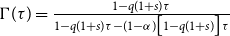


 Open access