


Introduction
Reliable and precise velocity measurements are a crucial factor for the operation of conventional and especially autonomous trains. There are well known, established possibilities for rather coarse velocity measurements. The most common is probably the tachometer which counts the number of wheel turns in a known time interval [Reference Kim and Han1]. For a known wheel diameter and a ride without slip this method provides precise velocity measurements. But as friction between wheel and rail is insufficient in situations of high acceleration a serious amount of slip occurs especially in crucial situations [Reference Monje, Aranguren, Martinez and Casado2]. But even in situations of constant velocity, the uncertainty regarding the current wheel diameter causes a proportional uncertainty in velocity measurements.
A more recent velocity measurement technique was enabled by the Global Positioning System (GPS). GPS offers an accuracy of down to 0.01 m/s. This accuracy comes with the drawback of limited availability in tunnels as well as in urban areas with high buildings [Reference Enge3].
Common radar-based velocity measurements exploit the Doppler effect [Reference Heide, Magori and Schwarte4]. This technique exploits the simple relationship between train velocity and the receive signal frequency. The precision of Doppler-based measurements is essentially limited by the unknown ground clutter in combination with the unavoidable wide beam width of the radar antenna. Furthermore, this technique lacks precision in the range of low velocities [Reference Xiang, Lin and Wanhai5]. This is especially unfavorable as the trains velocity has to fall below a certain value before the doors are opened.
In a real train scenario, most of the aforementioned systems are used in parallel. In the EU the accuracy and reaction time requirements for the whole on-board velocity measurement system are defined in [6]. This document states that the acceptable deviation for the measured velocity is limited to 2 km/h for velocities below 30 km/h and increases linearly up to a deviation of 12 km/h for a velocity of 500 km/h. Due to the low acceleration and deceleration potential of trains in general, the maximum reaction time is defined to be 1 s. These requirements are used as the main reference for this work.
In [Reference Laqua7] a very similar approach for general vehicle velocity estimation is introduced. However, the theoretical considerations assume that there is an only slightly rough underground present. This is clearly not the case for the track bed beneath a train.
This paper introduces a novel approach for the measurement of train velocities. It is based on the correlation of two images recorded with a spatial offset. The section “Terrain pattern correlation” presents the measurement approach which is based on the correlation of two radar images. It also investigates if the additional use of a synthetic aperture radar (SAR) [Reference Nicolas and Adragna8] leads to any advantage in this application. Therefore in the section “Radar imaging basics” the basics of radar imaging are introduced. The section “Test measurements” presents the first results which are gathered by performing lab measurements. In the section “Field measurements” the results of field measurements with a train are presented. The section “Discussion” discusses the differences of some ideal assumptions, the test measurement conditions and the field measurement conditions.
Radar imaging basics
A FMCW-Radar sends a linear frequency chirp of the form
 $$s(t) = {\rm rect}\left( {\displaystyle{t \over T}} \right)\cos (2\pi f_0t + \pi k_Ct^2), $$
in which T denotes the chirp duration, k C is the chirp rate, and f 0 is the base frequency. The chirp bandwidth is defined as B = k C · T. This signal may be reflected by an isotropic point scatterer at the distance r with radar cross-section σ. Mixing the received signal and the transmitted signal and low-pass filtering the result yields
 $$\eqalign{ h(r,t) & = \sigma {\rm rect}\left( {\displaystyle{{t-r/c} \over T}} \right)\exp \left( {\,j4\pi \displaystyle{r \over c}\left[ {\displaystyle{{\,f_0} \over {k_C}}-\displaystyle{r \over c}} \right]} \right) \cr & \quad \exp \left( {-j4\pi k_C\displaystyle{r \over c}t} \right).} $$
Neglecting constant coefficients, this reads in the Fourier domain as
 $$ H(r, f) = \sigma \, L(r, f) $$
 $$ L(r,f) = {\rm sinc} \left( {T\left( {\,f-\displaystyle{{2r} \over c}k_C} \right)} \right)\exp \left( {-j2\pi \displaystyle{r \over c}\left( {\,f-2f_0} \right)} \right). $$
in which L(r, f) denotes the frequency response coefficient of a target at a distance r.
As can be seen, the Fourier transform of the received signal contains information about the reflectivity of a target in a certain distance. Moving the radar perpendicular to the main beam direction offers the possibility to create maps which illustrate the reflectivity of targets on a two-dimensional plane. This measurement principle applied to the presented problem is depicted in Fig. 1.
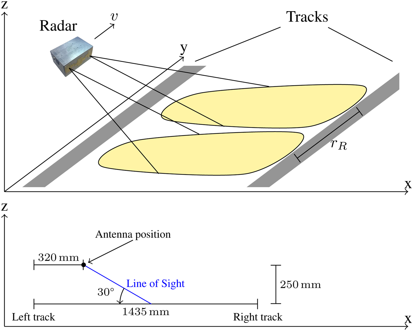
Fig. 1. The upper part shows the measurement situation schematically. The marked areas are scanned simultaneously by the two radar receivers [Reference Reissland, Lenhart, Lichtblau, Sporer, Weigel and Koelpin9]. The lower part shows the measurement geometry true to scale.
While moving in y-direction with velocity v, the radar emits pulses at a certain rate, the pulse repetition rate f PRF. Due to the rather wide antenna beam, every chirp is reflected by a set of scatterers. This causes a low-pass effect on the generated image in moving direction. This low-pass effect can be compensated by applying a matched filter to the generated data. This technique is also called azimuth compression. The matched filter can be described in Fourier domain as
 $$\eqalign{& H_A(\,f) = \exp \left( {-j\pi \displaystyle{{\,f^2} \over {k_A}}} \right) \cr & \quad k_A = -\displaystyle{{2v^2} \over {\lambda R_0}}.} $$
R 0 denotes the shortest distance to a ground line parallel to the y-axis. The matched filter function depends, among other parameters, on the velocity of the vehicle. In the formation of the SAR image a range cell migration correction (RCMC) is needed. The RCMC approach used in this work is described in [Reference Raney, Runge, Bamler, Cumming and Wong10]. The resulting image is subsequently denoted as I(m, n), index n refers to the image pixel index in range direction, whereas m refers to the moving direction. The function which calculates the image is called SAR(v) [Reference Richards, Holm and Scheer11].
Terrain pattern correlation
To apply the terrain pattern correlation, two coherent receivers are placed at a known distance r R in y-direction apart from each other. As the train is moving the two receivers will pass the same spot on the ground with a temporal difference Δt = r R/v.
When the two receivers pass the same spot on the ground they will receive the same reflections and therefore generate the same image. The image generated by the first and second radar is named i 1(m, n) and i 2(m, n), respectively.
The image formation for receiver 1 and receiver 2 is formulated in equations (6) and (7), respectively. It can be described as a surface integral over the observed ground area. For the sake of simplicity, the formulation is done in the continuous spatial and frequency domain.
 $$ \eqalign{ i_1(y_R,f) = &\mathop{\islant 20%\int\!\!\islant 20%\int}\limits_A {\sigma _{xy}} (x,y)\cdot G_{RX}\left( {x,y-\left( {y_R + \displaystyle{{r_R} \over 2}} \right)} \right) \cr &\cdot G_{TX}(x,y-y_R)\cdot L(r,f)\; dx\; dy,} $$
 $$ \eqalign{ i_2(y_R,f) =& \mathop{\islant 20%\int\!\!\islant 20%\int}\limits_A {\sigma _{xy}} (x,y)\cdot G_{RX}\left( {x,y-\left( {y_R-\displaystyle{{r_R} \over 2}} \right)} \right) \cr &\cdot G_{TX}(x,y-y_R)\cdot L(r,f)\; dx\,\; dy,} $$
 $$ r = \sqrt{x^2 + y^2 + z_0^2}. $$
In these formulae G RX and G TX denote the projection of the antenna diagrams onto the ground for the receive antennas and the transmit antenna. The infinitesimal reflectivity of the ground is called σ xy. y R denotes the position of the transmit antenna in y-direction. The transmit antenna is assumed to be located in the middle between the two receive antennas. These formulations therefore take into account the geometry of the imaging process.
The relation between continuous frequency domains and the discrete domain can be specified by
 $$f = \displaystyle{n \over {T_{PRF}}}, $$
if one assumes that T PRF is the length of the time domain signal processed by the FFT, i.e. the time domain signal is processed without performing zero padding. In the spatial domain the relation is given by
 $$ y_R = m \cdot v \cdot T_{PRF}, $$
for a constant velocity v and T PRF = 1/f PRF.
The discrete index versions of the images can therefore be expressed as
 $$I_1(m,n) = i_1\left( {m\cdot v\cdot T_{PRF},\displaystyle{n \over {T_{PRF}}}} \right) $$
 $$I_2(m,n) = i_2\left( {m\cdot v\cdot T_{PRF},\displaystyle{n \over {T_{PRF}}}} \right). $$
It has to be mentioned that these images are formed without the matched filtering in y-direction introduced by equation (5). Adjacent pixels in y-direction are recorded with a temporal difference of T PRF. This discrete index relationship of the two images can be formulated as
 $$I_1\left( {m + \displaystyle{{\Delta t} \over {T_{PRF}}},n} \right) = I_2(m,n), $$
assuming Δt = LT PRF, L ∈ ℕ. The pixel distance will subsequently be denoted as Δm = Δt/T PRF. Δm can therefore be understood as the number of chirps transmitted within the time the two radars need to pass a certain spot. The actual train velocity can be calculated as
 $$v(\Delta m) = \displaystyle{{r_R} \over {\Delta m\; T_{PRF}}}.$$
To estimate Δm, the peak of the cross-correlation function [Reference Bronstein, Semendjajew, Musiol and Mühlig12] between the images I 1 and I 2 has to be found. The cross-correlation function is calculated as
 $$C(\Delta {\widetilde m}) = \displaystyle{{\sum\nolimits_{n = 1}^N {\sum\nolimits_{m = 1}^M \vert } I_1(m,n)\vert\vert I_2(m + \Delta {\widetilde m},n)\vert} \over {\sqrt {\matrix{\sum\nolimits_{n = 1}^N {\sum\nolimits_{m = 1}^M \vert } I_1(m,n)\vert^2 \cdot \sum\nolimits_{n = 1}^N {\sum\nolimits_{m = 1}^M \vert } I_2(m + \Delta {\widetilde m},n)\vert^2} }}}$$
 $$\Delta \widehat{m}{\rm } = \mathop{\rm argmax}_{\Delta {\widetilde { m}}}C(\Delta {\rm }{\widetilde m}). $$
 The before mentioned estimate is denoted by  $\Delta \widehat {m}$. The variable M also referred to as image size will be of certain importance. It denotes the number of chirps which are taken into account for the calculation of the correlation.
An advantage, compared to other velocity measurement techniques such as the Doppler radar is that the reliability of the measured velocity can be quantified by evaluating C(Δm). This enables the use of soft-decision sensor fusion algorithms in case there are several velocity measurement systems available.
Up to here, it was assumed that optimally processed SAR images of the terrain are available for the terrain pattern correlation. However, as was mentioned in the section “Radar imaging basics”, the SAR signal processing needs information about the actual vehicle velocity. As this information is obviously not available it has to be tested if the algorithm still works without the resolution enhancement provided by the SAR processing steps.
The whole processing chain is depicted in Fig. 3. The hamming windowing for sidelobe reduction as well as the fast Fourier transform (FFT) in the range dimension are basic processing steps in the FMCW radar processing. Its result is a 2D image with only course resolution in azimuth direction. The three following steps include the actual SAR processing and will lead to an image with enhanced azimuth resolution. They are marked as optional because they have to be omitted in the real application. The 2D image contains areas in which no usable data can be expected. These include the area between the receiver and the nearest spot on the ground, as well as area, which lies further away than the opposite track. Discarding these informations leads to reduced computational cost. The last three processing steps are already thoroughly discussed in this work.
The inherent limits regarding the accuracy and reaction time depend on the trains real velocity v, the receive antenna distance r R, and the chirp duration T PRF. The first limit is denoted as velocity resolution, it presents a lower limit for the velocity measurement accuracy. As Δm ∈ ℤ, the velocity resolution is not infinitely fine. The normalized velocity resolution is defined as
 $$\eqalign{\displaystyle{{\Delta v} \over v} &= \displaystyle{{v(\Delta m)-v(\Delta m + 1)} \over {1/2(v(\Delta m) + v(\Delta m + 1))}} \cr& = \displaystyle{2 \over 2 \left({r_R /vT_{PRF}}\right) + 1}.} $$
As can be seen from equation (17) the achievable resolution is limited by the PRF if the receive antenna distance r R is fixed. In our current field measurement system r R is 17 cm and the PRF is set to f PRF = 1 kHz. With these parameters the field measurement system meets the requirements stated in [6] up to a velocity of 36 km/h. To meet these requirements for velocities up to 500 km/h the PRF will have to reach about 40 kHz. A comparison of the velocity resolutions for the two PRFs, complemented by the requirements, is depicted in Fig. 2. For the test measurement setup these considerations are of no concern as the maximum achievable velocity here is limited to below 0.5 km/h.
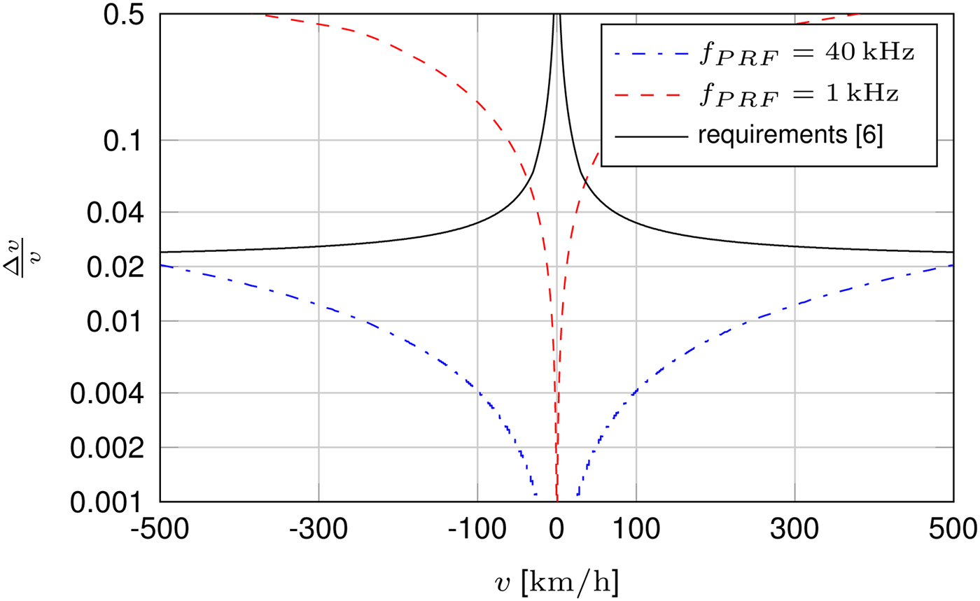
Fig. 2. Normalized velocity resolution of the terrain pattern correlation for r R = 17 cm and two different PRFs.
The second inherent limit of the method affects the reaction time of the system. To correctly correlate the two receivers images, the second receiver has to pass over the same area that the first receiver already imaged. For this the train has to move by the distance r R, therefore the reaction time can simply be calculated as
 $$T_r = \displaystyle{{r_R} \over v}. $$
For the already mentioned field measurement setup T r exceeds the reaction time requirement of 1 s for v ≤ 0.612 km/h.
Test measurements
In order to evaluate the proposed algorithms, several test measurements were carried out in a laboratory environment. To imitate a moving train, the measurement system is mounted on a 3 m long linear stage. The measurements are carried out by a bi-static 24 GHz FMCW radar, depicted in Fig. 4. The FMCW signal parameters are set to T PRF = 90 ms, B = 1.5 GHz, and therefore k C = 16.6 GHz. The antennas main beam width is Θ A = 57° in moving direction. The sensor is leaned by 45° towards the ground. The utilized Horn antennas have an antenna gain of 10 dBi. The distance between sensor and targets ranges from 0.5 to 1.5 m.
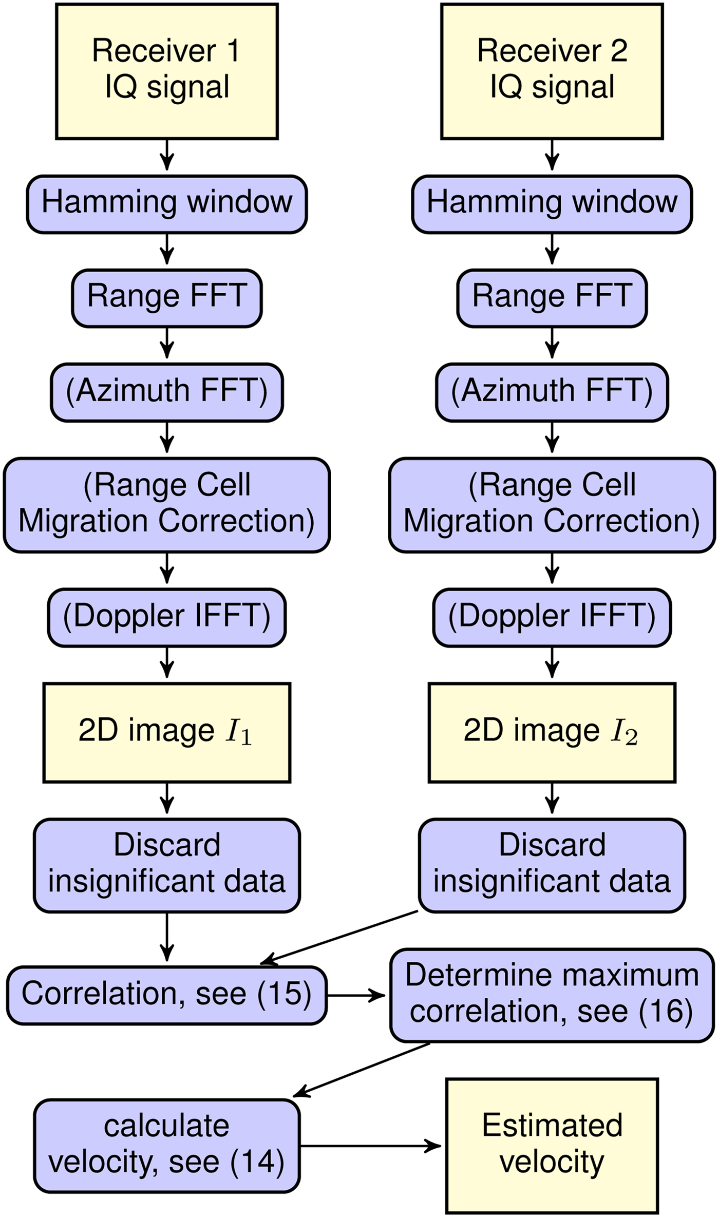
Fig. 3. Processing sequence from raw data to velocity estimates.
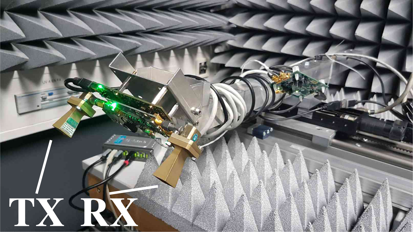
Fig. 4. Radar Sensor used for tests [Reference Reissland, Lenhart, Lichtblau, Sporer, Weigel and Koelpin9].
From these parameters the resolutions of the SAR imaging radar can be determined. The range resolution can be calculated by the well-known relationship
 $$\Delta R_R = \displaystyle{c \over {2\cdot B}} = 10\; {\rm cm}. $$
According to [Reference Richards and Richards13] the azimuth resolution can be approximated by
 $$\Delta R_A = \displaystyle{c \over {4f_c\cdot \tan (\Theta _A/2)}} = 5.7\; {\rm mm}.$$
Two different types of target scenarios are investigated in the measurements. The first one is shown in Fig. 5, it consists of several distinct targets. The second scenario refers to the real-world problem, as a track bed is imitated by a field of crushed rocks on the floor, as can be seen in Fig. 6. All measurements were carried with a constant velocity.
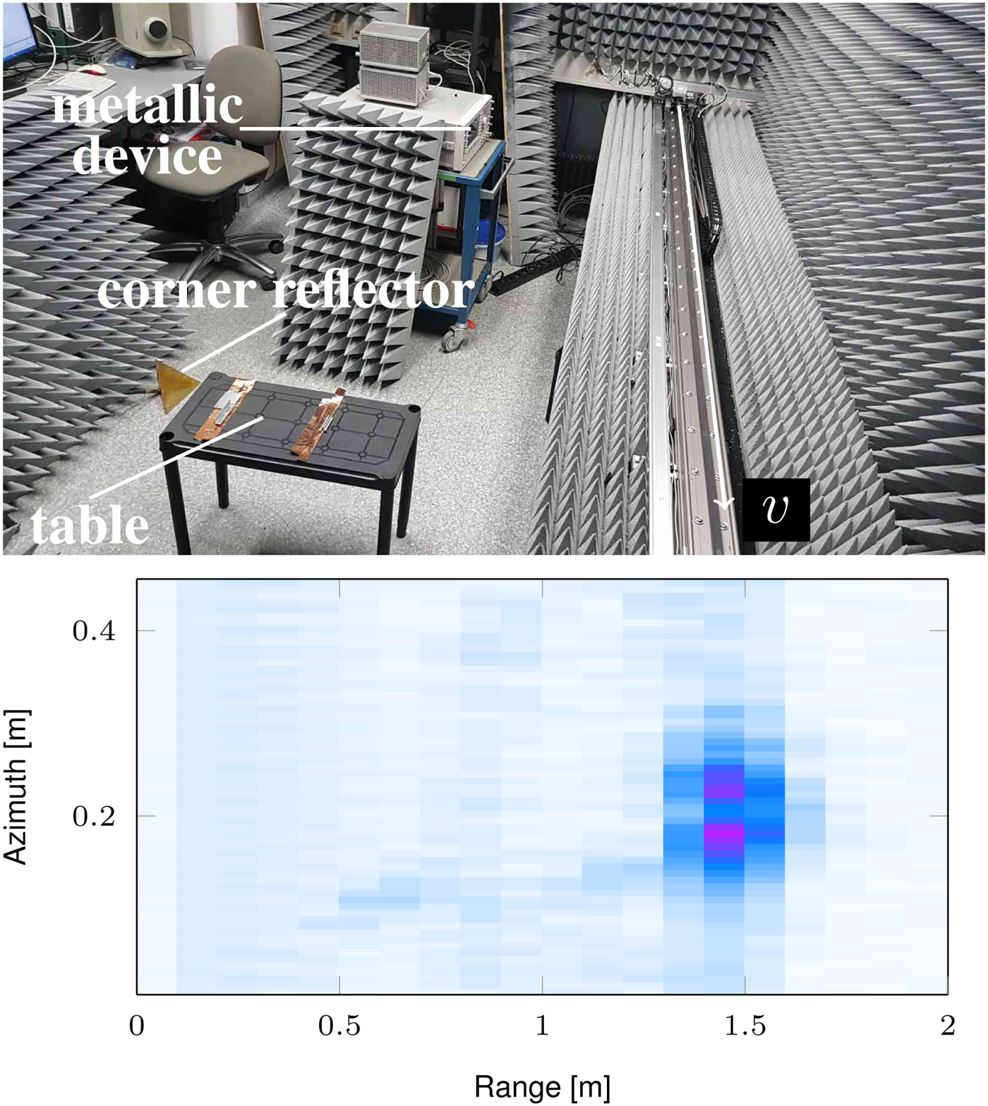
Fig. 5. Scenario one, installation with distinct targets [Reference Reissland, Lenhart, Lichtblau, Sporer, Weigel and Koelpin9]. The lower part shows a corresponding SAR image for which also the azimuth compression was carried out. The dark spot is caused by the corner reflector.
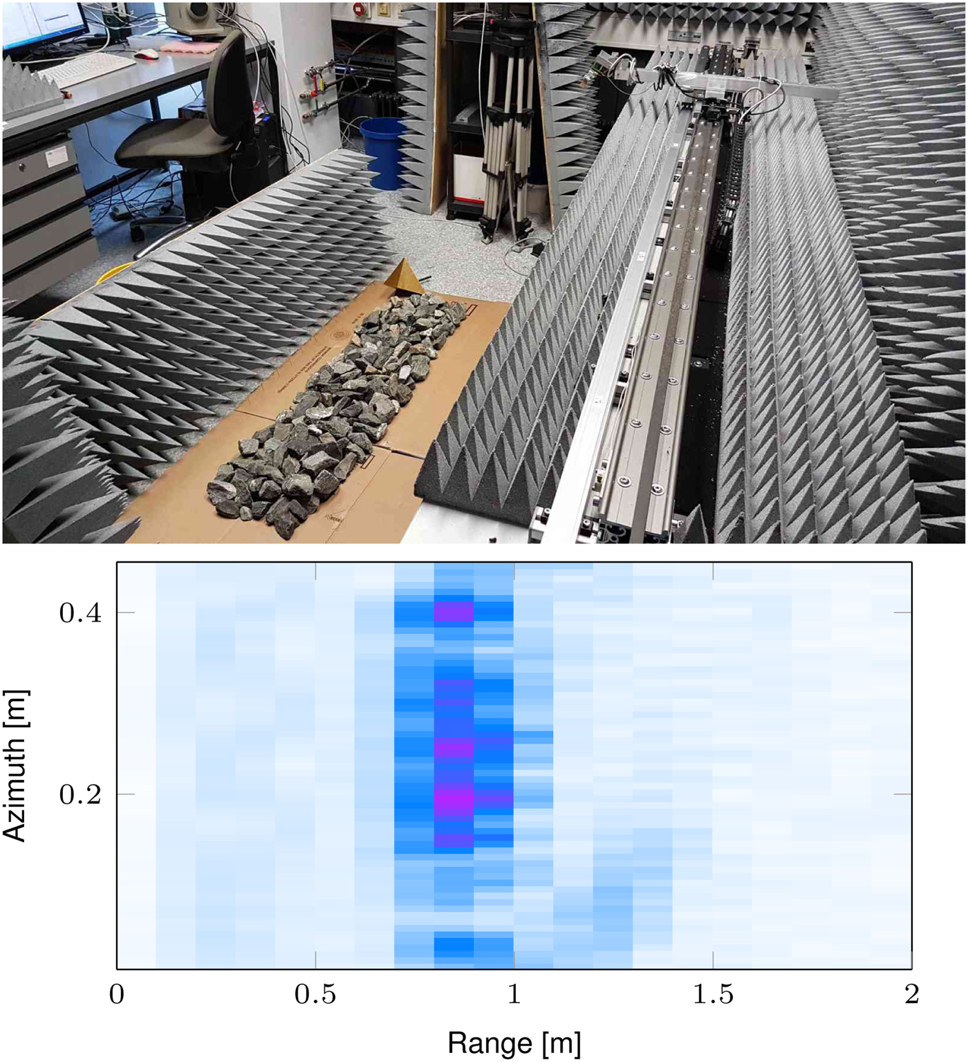
Fig. 6. Scenario two, installation with realistic targets. The linear stage is shown on the right-hand side [Reference Reissland, Lenhart, Lichtblau, Sporer, Weigel and Koelpin9]. The lower part shows a corresponding SAR image for which also the azimuth compression was carried out.
It is important to mention, that only one radar sensor is used. The data for the second sensor are generated by repeating a measurement and adding a pixel distance Δm. The same distance should be found by the correlation peak search. By performing two independent measurement rides it is ensured that the data are not recorded at the very same positions. This disturbance also occurs when the train is moving and r R/v T PRF is not an integer, which is usually the case.
The goal of the measurements was to verify the concepts of the proposed algorithm. The first challenge was to reconstruct the introduced distance Δm. As was already mentioned this distance corresponds to the velocity in the application. Neglecting the already given disturbances, I 2 is a delayed version of I 1. Therefore, the cross-correlation function should exhibit the same convex behavior as an auto-correlation function. Verifying this property is the second goal regarding the terrain pattern correlation. The third and most important question is how well the algorithm performs if the velocity is not a-priori known and the SAR processing steps cannot be applied.
The measurements for both scenarios are done with different stage velocities, ranging from 4.69 to 11.75 cm/s. The effect of different velocities on the results is insignificant, therefore only the results for the highest and hence most challenging velocity are presented.
For all of the algorithmic tests the pixel delay Δm is set to 30. The correlation functions of the first scenario are depicted in Fig. 7. As can be seen the correlation maximum, with and without azimuth compression, is located exactly at Δm = 30. Without applying the azimuth compression, the region around the peak is slightly less steep, the peak search is therefore more vulnerable to noise disturbances. Also, the correlation function is convex, therefore more efficient search algorithms for the peak, than exhaustive search, can be applied.
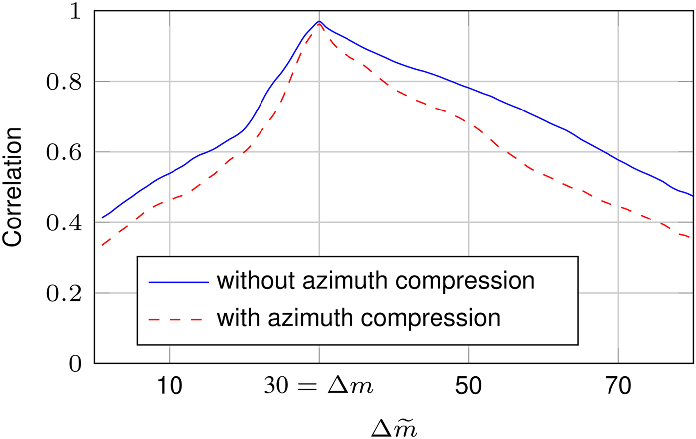
Fig. 7. Results of the terrain pattern correlation for the first scenario with Δm = 30 and v = 11.75 cm/s [Reference Reissland, Lenhart, Lichtblau, Sporer, Weigel and Koelpin9].
The results for the second scenario are depicted in Fig. 8. Again, the correlation peak is located at the correct position, therefore, disregarding the limited resolution, the measured velocity is the correct one. In contrast to scenario one, the distinctiveness of the correlation maximum is not altered by the azimuth compression.
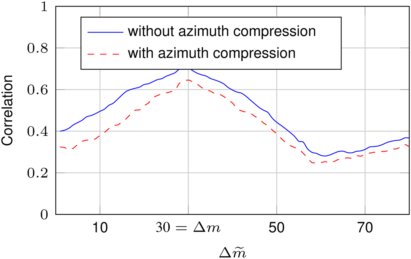
Fig. 8. Results of the terrain pattern correlation for the second scenario with Δm = 30 and v = 11.75 cm/s [Reference Reissland, Lenhart, Lichtblau, Sporer, Weigel and Koelpin9].
According to [Reference Nicolas and Adragna8] speckle can be observed in SAR images if a high number of scatterers is present, which is only true for the second scenario. This speckle introduces differences in the two recorded images. This in turn will lower the overall correlation for the SAR processed image. Also, the slope of the correlation in the second scenario is less steep. This is caused by the fact that shifting the image in moving direction will cause less changes in the image of the second scenario. This can be well observed in Figs 7 and 8. Anyway, the peak is clearly visible in both cases and the convex nature of the correlation function is also visible, at least up to a certain deviation from Δm. Regarding the robustness against strong noise the value of the maximum correlation is of no concern. Only the correlation value of the maximum correlation compared to the neighboring ones is important for the methods robustness against noise disturbances.
As mentioned above, as long as the correct correlation peak is found, the precision of the measured velocity is only limited by the pulse repetition frequency. However, this does not mean that the precision can be arbitrarily improved by increasing the pulse repetition frequency. This is caused by the fact that nearby image pixels get more similar with increasing pulse repetition frequency. This in turn will result in wrongly determined pixel distances Δm.
Regarding the systems accuracy two influences have to be mentioned. The first one is again the pulse repetition frequency. If it is not known exactly, the deviance will cause a velocity dependent bias in the measurements. The second major influence is the angle of the antenna beam. If one or both antennas are unintentionally squinting, this will influence r R and will therefore also lead to a velocity-dependent deviance.
Field measurements
To carry out field measurements a radar system with two receive antennas is needed. This system is depicted in Fig. 9. It is equipped with an ethernet interface which was connected to a PC during the measurements. The processing of the raw data is carried out offline in Matlab.
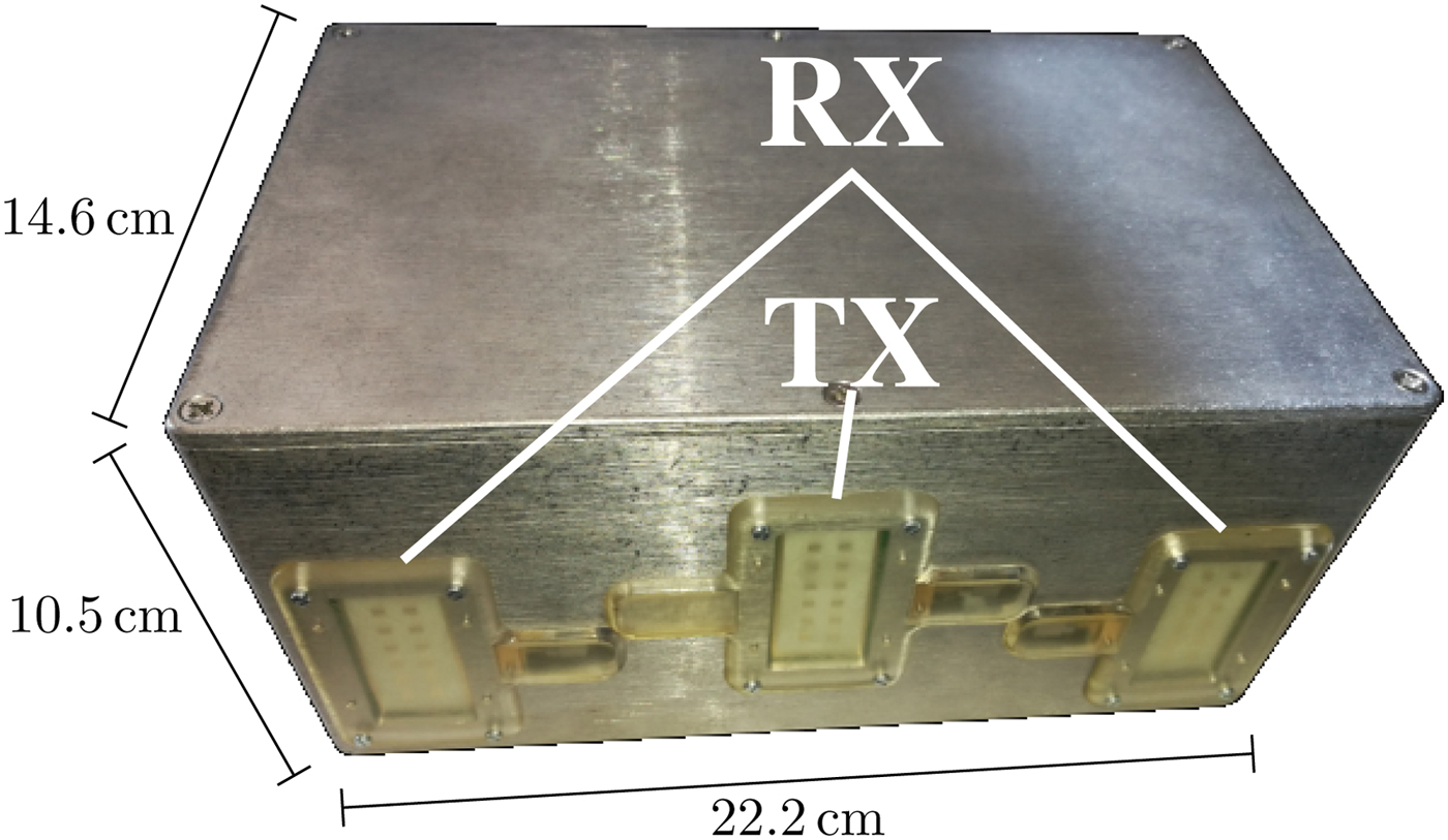
Fig. 9. Radar System used for field measurements. The horizontal distance between the transmit antenna and each of the receive antennas is 8.5 cm.
Unlike the measurement principle shown in Fig. 1 suggests the actual system does not consist of two monostatic radars, but one radar with two receive antennas. This approach offers the advantage of a doubled pulse repetition frequency because the use of two independent radar sensors would force the utilization of time division multiplexing to avoid signal interference. The frontend and baseband hardware is the same as was used in the test measurements. The chirp interval is decreased to T PRF = 1 ms, which is the minimum interval for the employed frontend. Measurements were carried out with two different chirp bandwidths. First the same bandwidth B = 1.5 GHz as was used in the test measurements was used. Later the bandwidth was reduced to B = 250 MHz to investigate if the approach still works if the radar only transmits within the 24 GHz ISM band. The employed antennas each consist of a 2 × 6 patch-array offering a 3 dB angular width of 42.4° in horizontal direction.
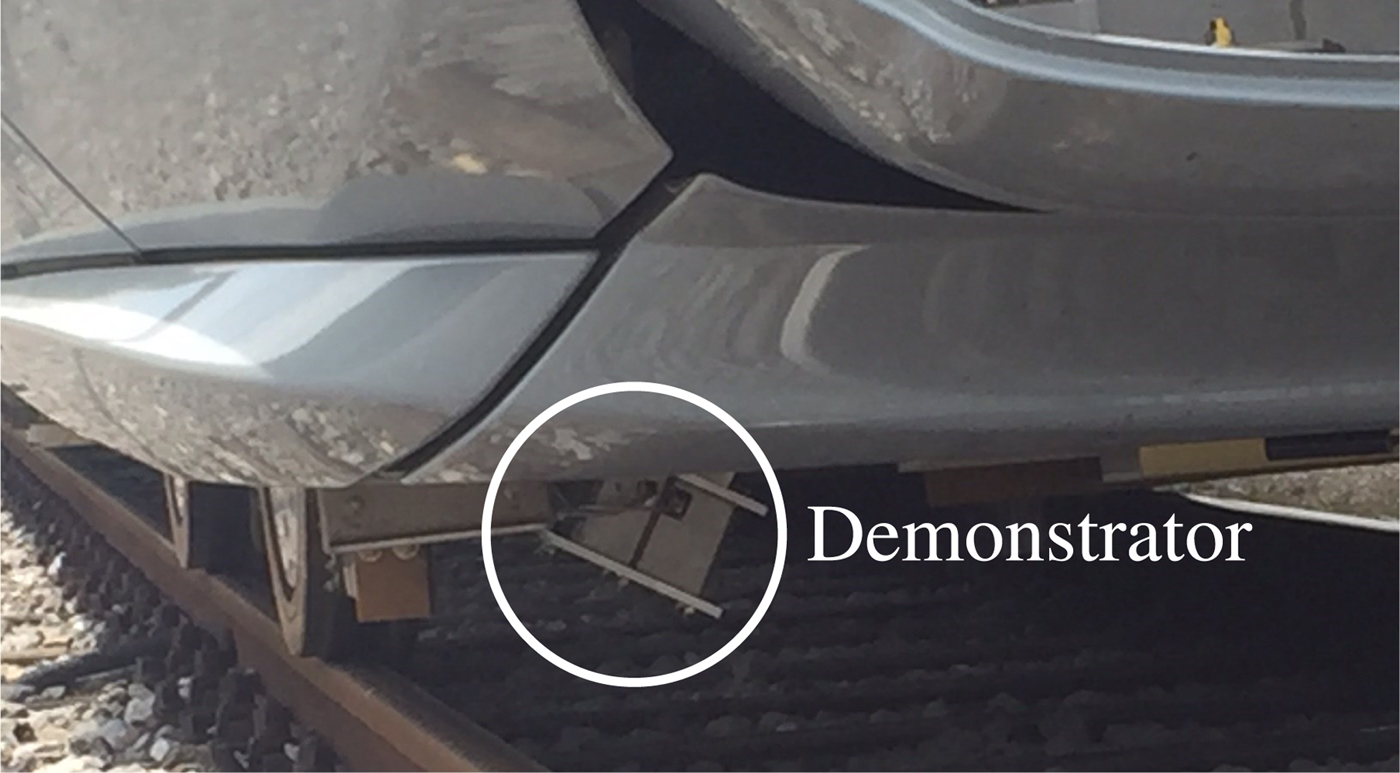
Fig. 10. Field measurement system mounted on a train.
While carrying out the field measurements it was not possible to record reference data from the trains conventional velocity measurement systems due to restrictions nor from an independent GPS module due to the high attenuation of GPS signals inside the train. Therefore manually taken records of the tachometer values serve as a basis for the data evaluation. The respective records are stated below the corresponding Figs 11, 12 and 13.
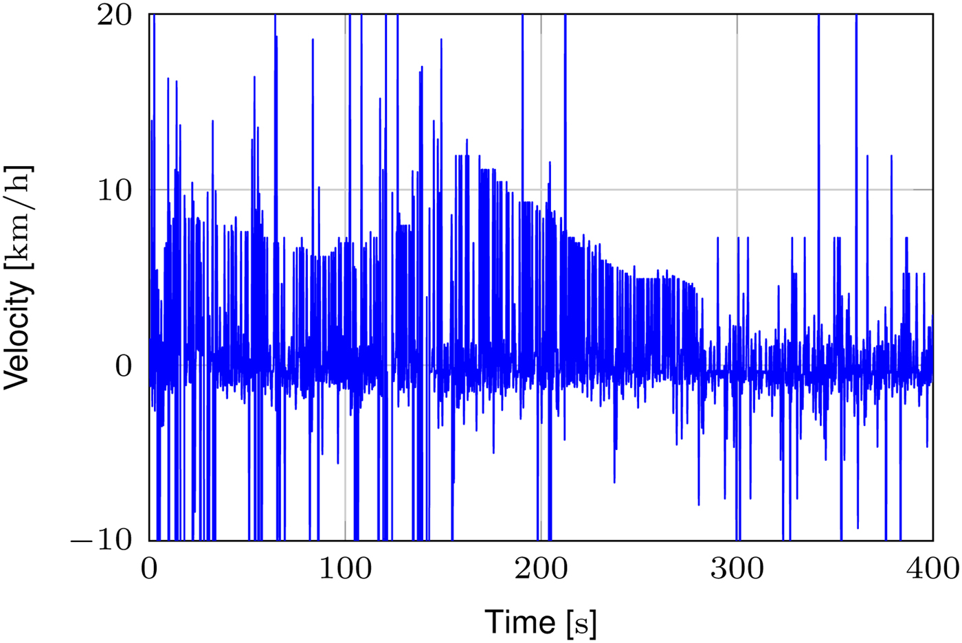
Fig. 11. Measured velocity when the train drove at a low, non-constant velocity. After about 300 s the velocity was reduced to 0 km/s. The parameters for this measurement are B = 1.5 GHz and M = 256.
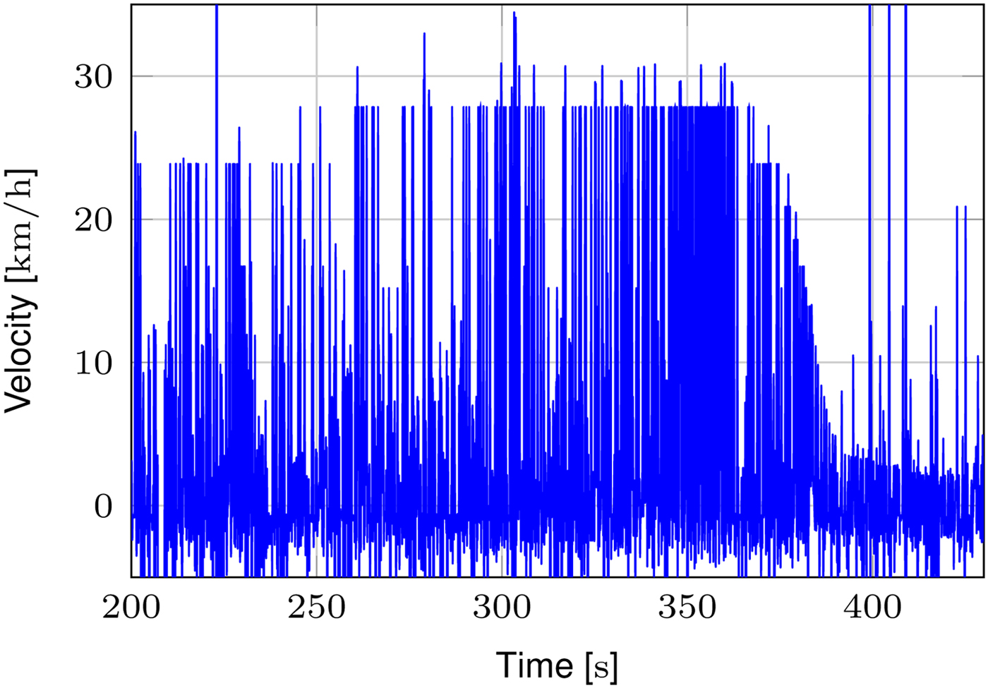
Fig. 12. Detail of a run in which the train drove at about 25 km/h. At the end it slowed down until standing. The parameters for this measurement are B = 1.5 GHz and M = 128.
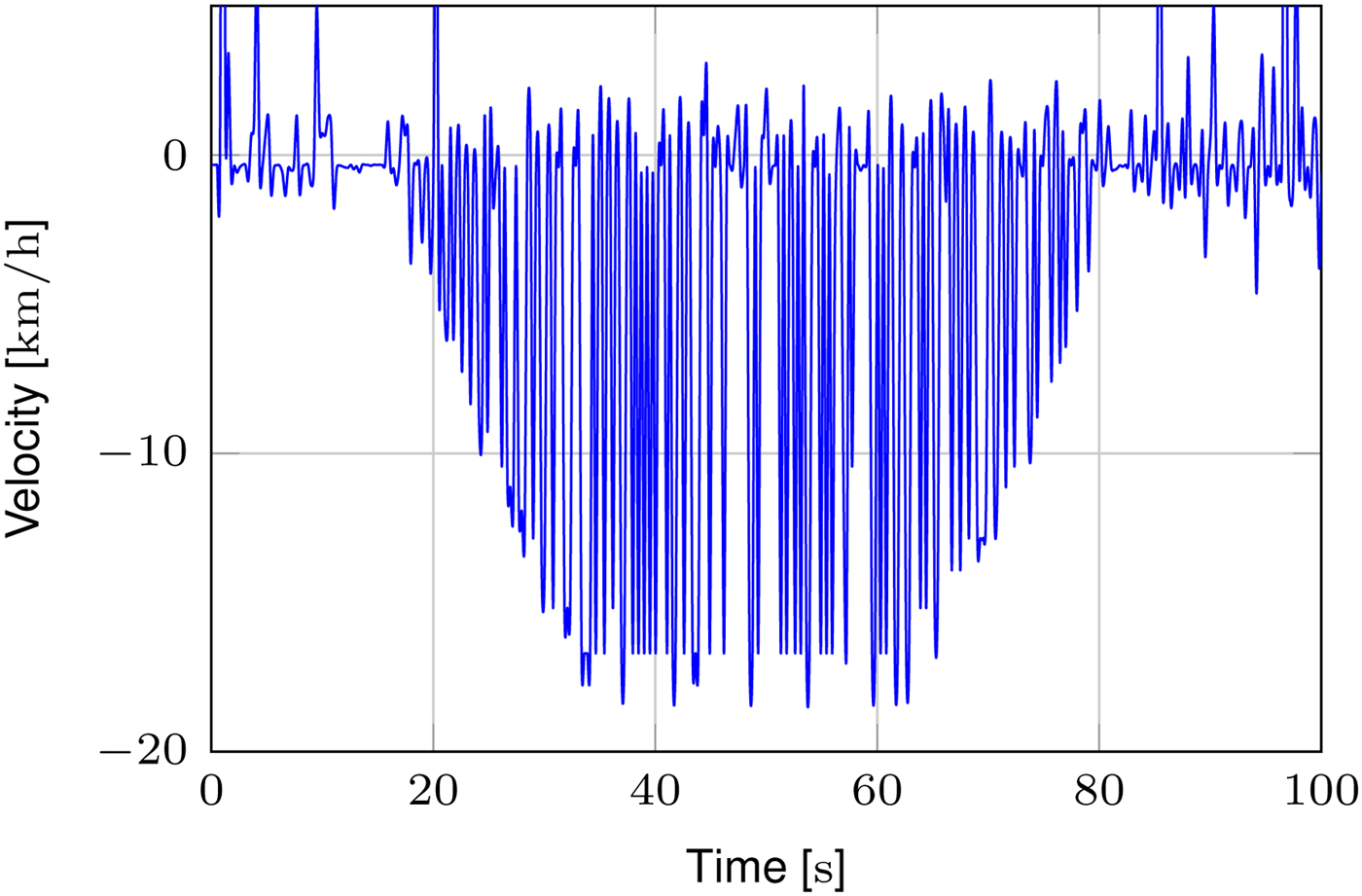
Fig. 13. A run in which the train was driving in negative direction, accelerating and decelerating. The parameters for this measurement are B = 250 MHz and M = 256.
One aspect of interest in the evaluation of the field measurements is the influence of the image size M on the results. Increasing the image size leads to an increased SNR. Also the probability that significant structures on the ground appear within an image is increased. On the other hand, if the train is accelerating or decelerating while the image is recorded, the assumption of a nearly constant velocity during the measurement is violated. Furthermore, the reaction time of the algorithm increases with the image size, as more data has to be recorded, prior to the actual processing. Therefore it is important to find a proper image size by evaluating the same data with a number of different image sizes. The image sizes regarded in the evaluation are M ∈ {32, 64, 128, 256, 512}.
For M ∈ {32, 64} the velocity output shows only a very limited number of measurement results in the expected velocity range. Therefore these measurements are not depicted here. Useful measurement data are achieved if the image size is set to M = 128. An example for this is illustrated in Fig. 12. Even though there are still a lot of apparently invalid measurements the velocity curve is clearly visible. This figure is also chosen as it shows the effect of limited velocity resolution. This is the reason the velocity seems to be constant in the time range from about 270 s to about 370 s.
When the image size is further increased to M = 256 there is still some visual improvement of the measurement data. An example for this case is depicted in Fig. 11. The velocity curve is clearly visible, also the velocity resolution is enhanced, which is due to the lower observed velocities. In Fig. 13 a measurement performed with a bandwidth of only 250 MHz is depicted. In this case, no visible degradation is observed, the velocity curve is still clearly visible.
For M = 512 no further enhancement is observed. One limit of the approach is also visible in the figures. It is not possible to retrieve a useful velocity measurement if the train is standing still. However, this does not affect the overall usefulness as this condition can be easily determined by comparing the receive signals over slow time.
Discussion
To understand the differences between the relation of the ideal images as stated in equation (13) and the relation between the images taken by the field measurement system, the imaging process has to be investigated.
As can be implied from equations (7) and (9) the receive antennas cover the same ground area if y R is shifted by r R, i.e. if the train moved as far as the receive antennas are separated by each other. In contrast to this, the transmit antenna illuminates the same ground area differently if y R is shifted by r R. This becomes obvious as in general
 $$ G_{TX}\left( {x,\displaystyle{{r_R} \over 2} + {\epsilon }} \right)\ne G_{TX}\left( {x,-\displaystyle{{r_R} \over 2} + {\epsilon }} \right), $$
for any real value ε. To diminish the implications of this effect the beamwidth of the transmit antenna should be as wide as possible. This will usually lead to lesser variations of G TX around the area in front of the receive antennas. On the contrary, the receive antennas beamwidths should be as narrow as possible for two reasons. First, a more narrow receive antenna beamwidth means smaller weighting of areas where there are larger G TX variations among the passes of both receive antennas. Second, a wider receive antenna beamwidth will lead to a stronger spatial lowpass effect. This in turn attenuates the influence of rather small structures on the ground which would be useful for a significant correlation result.
One more reason for non-ideal correlation results is related to the one stated above. When an area is passed by receive antenna 1 it is illuminated from another angle when it is passed by receive antenna 2. The results of this effect are attenuated if the angular difference is kept as small as possible. This can be achieved by placing the receive antennas as close as possible to each other. On the other hand, as stated in equation (17) a closer spacing of these antennas will lead to a decreased velocity resolution, therefore a compromise has to be found.
Therefore to enhance the system towards a practical solution several measures will have to be taken. The first is a highly increased PRF which will lead to a better resolution at high velocities. The second measure will be the use of more focusing antennas to make use of smaller details in the ground structure. The last physical measure targets the issue of angle dependency. This can be solved by either using two receive antennas as alternately emitting transceive antennas or by mounting the receive antennas at an angle. Furthermore, several algorithmic measures could be taken. This would include Kalman filtering, a MLSE estimator for the velocity estimation and using the already known reliability of the velocity estimations.
Conclusion
In this paper, a novel velocity measurement approach for vehicles was presented. It mainly consists of two side-looking radar sensors mounted underneath a train. Both sensors simultaneously take radar images of the terrain between the tracks. Those images are shifted and correlated along the moving direction, which yields a cross-correlation function. The peak of the cross-correlation function indicates the time after which both sensors passed the same spot. By means of this temporal delay, a velocity can be calculated. The lab measurements showed promising results for the use in train scenarios. Furthermore, field measurements on a train were carried out. These measurements show the proof of concept for the new approach. Based on these results limitations and future improvement approaches were discussed. The main limiting factor of the measurement technique is the pulse repetition frequency.
 Torsten Reissland (S'16) received his B.Sc. degree in Computer Engineering from the Ilmenau University of Technology in 2013 and his M.Sc. in Electrical Engineering from the Friedrich-Alexander University Erlangen-Nuremberg in 2016. In 2016, he joined the Institute for Electronics Engineering, Friedrich-Alexander University Erlangen-Nuremberg, as a Research Assistant. His current research interests include signal processing of radar and interferometric systems with focuses on signal modeling and imaging.
 Bjoern Lenhart (S'17) received his B.Sc. and M.Sc. degree in electrical engineering from Friedrich-Alexander University Erlangen-Nuremberg, Germany, in 2014 and 2017. In 2017, he joined the Institute for Electronics Engineering, Friedrich-Alexander University Erlangen-Nuremberg, as a research assistant, where he is currently working towards the Ph.D. His research interests are focused on RF communications, signal processing, and algorithms.
 Johann Lichtblau (S'15) received his B.Sc. in International Production Engineering and Management and M.Sc. degree in Mechanical Engineering from the Friedrich-Alexander University Erlangen-Nuremberg in 2014 and 2015, respectively. In 2015, he joined the Institute for Electronics Engineering, Friedrich-Alexander University Erlangen-Nuremberg as an External Doctoral Student and entered Siemens as a System Engineer. Since 2017 he has been a Project Leader in Research and Development at Siemens Mobility Erlangen, Germany. His research interests are in the fields of wireless communication, radar technology, and industry 4.0.
 Michael Sporer (S'13) received his B.Sc. in Electrical, Electronics and Communication Engineering and his M.Sc. (hons) degree in Systems of Information and Multimedia Technology from the Friedrich-Alexander University of Erlangen-Nuremberg in 2010 and 2012, respectively. In 2013, he joined the Institute for Electronics Engineering, Friedrich-Alexander University of Erlangen-Nuremberg, Erlangen, Germany, as a Research Assistant. His research interests include radar signal processing, millimeter-wave antenna, and circuit design.
 Robert Weigel (S'88-M'89-SM'95-F'02) received the Dr.-Ing. and the Dr.-Ing.habil. degrees from the TU Munich, Germany. From 1996 to 2002, he was the Director of the Institute for Communications and Information Engineering, University of Linz, Austria, where, in August 1999, he co-founded the company DICE, which was then split into an Infineon Technologies (DICE) and an Intel (DMCE) company. Since 2002, he has been the Head of the Institute for Electronics Engineering at the University of Erlangen, Germany. Dr. Weigel is an Elected Member of the German National Academy of Science and Engineering and an Elected Member of the Senate of the German Research Foundation. He was an IEEE Distinguished Microwave Lecturer and the 2014 MTT-S President. He is an IEEE Fellow and an ITG Fellow, and he received the 2002 VDE ITG-Award, the 2007 IEEE Microwave Applications Award, the 2016 IEEE Distinguished Microwave Educator Award, the 2018 IEEE Rudolph E. Henning Distinguished Mentoring Award and the 2018 EuMA Distinguished Service Award.
 Alexander Koelpin (S'04-M'10-SM'16) received his doctoral degree in 2010, and his “venia legendi” in 2014 all with the University of Erlangen-Nuremberg (FAU), Germany. From 2005 to 05/2017 he was with the Institute for Electronics Engineering, FAU, Germany. Since 06/2017 he is professor and head of the chair for Electronics and Sensor Systems with the Brandenburg University of Technology Cottbus-Senftenberg, Germany. His research interests are in the areas of microwave circuits and systems, wireless communication systems, local positioning, and six-port technology. Furthermore, he serves as a reviewer for several journals and conferences, is co-chair of the IEEE MTT-S technical committee MTT-16, of the Commission A: Electromagnetic Metrology of U.R.S.I., and from 2012 to 2017 conference Co-Chair of the IEEE Topical Conference on Wireless Sensors and Sensor Networks. In 2016, he has been awarded the IEEE MTT-S Outstanding Young Engineer Award and in 2017 with the ITG Award of the German VDE.


 Open access