


1. Introduction
There are two components to ice-sheet motion: internal deformation (governed by ice rheology) and basal sliding (governed by basal properties and subglacial hydrology). The rheology of ice is dependent upon ice temperature and ice fabric (the orientation distribution of ice crystals) (Azuma, Reference Azuma1994). The ice fabric provides a record of past deformation and significantly influences the viscosity of ice during future deformation (Alley, Reference Alley1988). Our understanding of ice fabric within the polar ice sheets is primarily informed by measurements from ice cores underneath ice divides and domes, which have low ice velocities (Wang and others, Reference Wang2002; Fujita and others, Reference Fujita, Maeno and Matsuoka2006; Montagnat and others, Reference Montagnat2014). This geographic limitation on direct observations of ice fabric limits our understanding of how fabric impacts ice dynamics and suggests a need for new geophysical methods for investigating ice fabric and its dependence and influence on ice flow across different flow regimes.
Ice fabric anisotropy results in dielectric anisotropy (birefringence), which can be detected using polarimetric radar sounding (Hargreaves, Reference Hargreaves1977). However, similar to ice core fabric measurements, radar sounding studies of ice fabric have focused on slow-flowing regions of the ice sheets (Fujita and others, Reference Fujita, Maeno and Matsuoka2006; Drews and others, Reference Drews2012; Matsuoka and others, Reference Matsuoka, Power, Fujita and Raymond2012; Li and others, Reference Li2018). In recent years the Autonomous phase-sensitive Radio-Echo Sounder (ApRES) has become widely used by glacier geophysicists when they perform ground surveys. The ApRES was originally designed to estimate basal melt and vertical strain rates (Nicholls and others, Reference Nicholls2015) and has since been used to investigate englacial water storage (Kendrick and others, Reference Kendrick2018), englacial layer geometry (Young and others, Reference Young2018), and to invert for ice flow velocities (Kingslake and others, Reference Kingslake, Martin, Arthern, Corr and King2016). The ApRES has recently been used to conduct polarimetric radar sounding measurements in complex flow regions, with Brisbourne and others (Reference Brisbourne2019) focusing on ice rises in the Weddell sea sector of Antarctica.
As a phase-coherent radar system, polarimetric measurements from an ApRES can be used to determine ice fabric properties using a polarimetric coherence framework (Dall, Reference Dall2010; Jordan and others, Reference Jordan, Schroeder, Castelletti, Li and Dall2019). This phase-based method has previously been applied to airborne measurements from the POLarimetric Airborne Radar Ice Sounder (POLARIS) (Dall and others, Reference Dall2009; Vazquez-Roy and others, Reference Vazquez-Roy, Krozer and Dall2012), and a ground-based version of the Multi Channel Coherent Radar Depth Sounder (MCRDs) (Li and others, Reference Li2018). The method enables estimation of ice fabric properties in the horizontal plane, formulated in terms of a second-order orientation tensor which describes the crystallographic/c-axis orientation distribution (Woodcock, Reference Woodcock1977; Montagnat and others, Reference Montagnat2014). Using radar phase to directly estimate ice fabric represents a departure from past power-based analyses (Hargreaves, Reference Hargreaves1977; Fujita and others, Reference Fujita, Maeno and Matsuoka2006; Matsuoka and others, Reference Matsuoka, Power, Fujita and Raymond2012; Li and others, Reference Li2018), which can suffer from angular ambiguity when inferring the prevailing fabric orientation (Fujita and others, Reference Fujita, Maeno and Matsuoka2006; Matsuoka and others, Reference Matsuoka, Power, Fujita and Raymond2012).
The goal of this study is to assess the potential of using the ApRES and the polarimetric coherence method to estimate ice fabric within ice streams. Fabric in ice streams has previously been characterized through direct sampling (Jackson and Kamb, Reference Jackson and Kamb1997) or seismic measurements (Horgan and others, Reference Horgan, Anandakrishnan, Alley, Burkett and Peters2011; Diez and Eisen, Reference Diez and Eisen2015; Picotti and others, Reference Picotti, Vuan, Carcione, Horgan and Anandakrishnan2015; Smith and others, Reference Smith2017). These studies indicate that a range of different fabric types can form in ice streams and there is a general lack of consensus regarding what is ‘typical’ ice-stream fabric. In addition, ice-stream flow mechanics studies have inferred marked spatial variation in ice fabric along flow (Minchew and others, Reference Minchew, Meyer, Robel, Gudmundsson and Simons2018) and have highlighted the role of ice fabric in modifying marginal shear-stress (Jackson and Kamb, Reference Jackson and Kamb1997). Further quantifying the effects of ice fabric on fast ice flow is also an important precursor to introducing more complete physics into large-scale ice-sheet simulations (Hay, Reference Hay2017).
As a case study of the polarimetric coherence method applied to fast ice flow, we focus upon a ground-based traverse across Whillans Ice Stream, West Antarctica. The analyses enable us to estimate ice fabric in selected regions of the ice column and compare estimates in the near-surface (z ≈ 10–50 m) to deeper ice (z ≈ 150–400 m). The results indicate that ice fabric can develop across relatively small spatial scales in fast ice flow (both between measurement sites and within the ice column).
2. Experimental Method
2.1. Radar system
The ApRES is a FMCW (Frequency-Modulated Continuous-Wave) radar with bandwidth, B = 200 MHz and center frequency, f c = 300 MHz. The classical range resolution of ApRES is

≈ 0.43, where εice ≈ 3.15–3.18 is the (real, polarization-averaged) dielectric permittivity of ice and c is the vacuum radio-wave speed. The instrument also has the capacity to measure sub-range-resolution precision using a Vernier technique but we do not do so here. The instrument stores the de-ramped signal which has phase

where ϕt is the transmitted phase and ϕr is the received phase. The impact of signal de-ramping upon the coherence method is discussed later. An in-depth technical summary of the ApRES is provided by Brennan and others (Reference Brennan, Lok, Nicholls and Corr2014).
2.2. Radar survey and measurements
Our study is located on the downstream reaches of Whillans Ice Stream, on the Siple Coast of West Antarctica (Fig. 1) and bounded to the grid northeast by the suture zone with the neighboring Mercer Ice Stream. These two ice streams originate from separate catchments, and merge over Whillans Ice Plain. The streamlines, derived from velocity measurements (Rignot and others, Reference Rignot, Mouginot and Scheuchl2011, Reference Rignot, Mouginot and Scheuchl2017), illustrate the suture zone between ice streams that begins with the coalescence of Whillans and Mercer shear margins. The approximate location of a basal sticky spot (Luthra and others, Reference Luthra, Anandakrishnan, Winberry, Alley and Holschuh2016) is also marked. The ground-based ApRES survey consists of a traverse of ten sites collected on 12 December 2016 that cross the suture zone dividing the two ice stream trunks. The site numbering is from grid east to grid west increasing upstream toward the sticky spot. The ice thickness across the traverse ranges from z ≈ 715 m (Site 10) to z ≈ 810 m (Site 1).
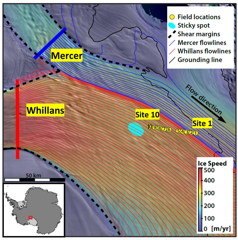
Fig. 1. Field setting of Whillans and Mercer ice streams on the Siple Coast, West Antarctica. The radar ground survey measurement sites are shown as numbered yellow dots. Streamlines from Whillans (red) and Mercer (blue) ice streams are derived from ice velocity (Rignot and others, Reference Rignot, Mouginot and Scheuchl2011, Reference Rignot, Mouginot and Scheuchl2017). Background image shows ice velocity over a mosaic of MODIS visible satellite imagery (Haran and others, Reference Haran, Bohlander, Scambos and Fahnestock2005).
At each site, co-polarized measurements (conducted with the transmit and receive antennas in the same orientation) were made using an established multi-polarization plane set-up (Fujita and others, Reference Fujita, Maeno and Matsuoka2006; Matsuoka and others, Reference Matsuoka, Power, Fujita and Raymond2012). This procedure consisted of measurements at a 22.5° angular resolution over the interval [0, 157.5]° with the azimuthal bearing angle, θ, defined as the angle between the polarization plane and due east in a counter-clockwise direction (Fig. 2). There are therefore eight independent polarization planes at θ = 0, 22.5, 45…157.5° which are indexed using i = 1, 2, 3…8. The horizontal baseline separation between receive and transmit antennas was approximately 10 m. During data collection θ was measured with respect to magnetic north/west, and was later corrected for magnetic declination (ranging from ≈100–120° east) to recover true north/west.
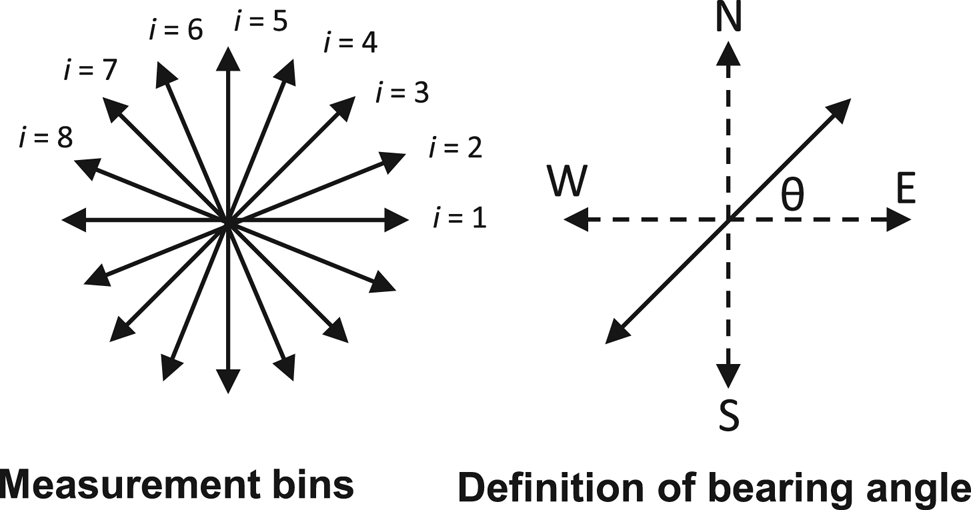
Fig. 2. (a) Multi-polarization plane measurements. (b) Definition of bearing angle.
2.3. Polarimetric data analysis
In this study we compare analyses of the polarimetric coherence alongside the polarimetric power and we now outline how these variables are computed from the ApRES data. A more detailed description of how these variables are related to ice fabric anisotropy is described in the Theoretical Background section.
2.3.1. Polarimetric coherence
When there is horizontal anisotropy in the ice fabric, polar ice behaves as a birefringent material for a vertically propagating radio wave. In this scenario, referred to as ‘birefringent propagation’, the radio wave polarizations experience different permittivities, travel at different phase velocities, and produce a polarimetric phase shift. The polarimetric coherence method provides a way to measure the polarimetric phase shift from sounding data and hence infer horizontal anisotropy in the ice fabric. A full description of the method is given by Jordan and others (Reference Jordan, Schroeder, Castelletti, Li and Dall2019), with Dall (Reference Dall2010) providing the initial proof-of-concept.
The method works by cross-correlating orthogonal co-polarized radar signals, s hh and s vv, and measuring the relative phase shift as a function of ice depth. When applied to multi-polarization plane data, the polarimetric coherence method pairs separate co-polarized measurements at 90 degrees, and considers the azimuthal behavior of the phase shift to infer the principal axes. Following Jordan and others (Reference Jordan, Schroeder, Castelletti, Li and Dall2019) we assume the convention that when θ = 0° the h polarization plane is aligned with the x-axis and the v polarization plane is aligned with the y-axis (i.e. bins 1 and 5 in Fig. 2 are paired). h−v polarization pairs are then generated as a function θ by pairing bins 2 and 6, 3 and 7, and 4 and 8 giving four independent pairs (Fig. 3).
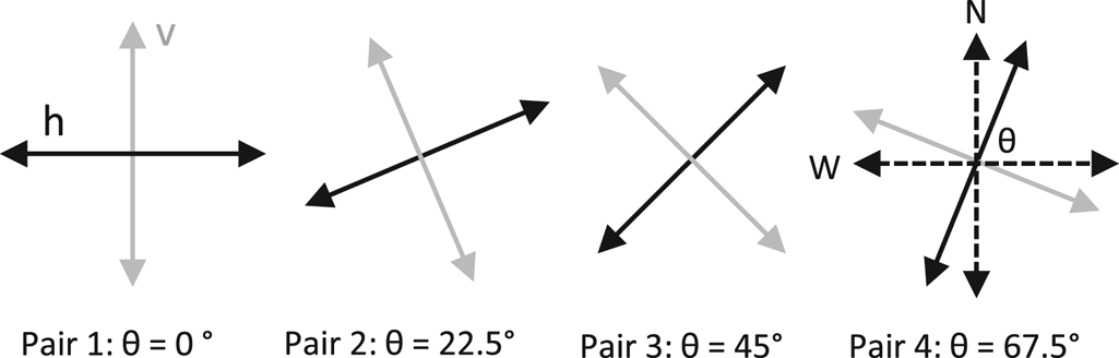
Fig. 3. Definition of h−v pairs in polarimetric coherence calculations.
For each h−v polarization pair the polarimetric coherence (also called hhvv coherence) is computed over a local depth window using the estimator
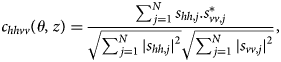
where N is the number of independent range bins, j is a summation index, $^\ast$ indicates complex conjugate, and the double subscripts indicate co-polarized measurements. c hhvv is a complex number defined within the unit circle. The coherence magnitude, |c hhvv| is defined on [0,1] and quantifies the correlation between hh and vv measurements. The hhvv coherence phase
provides a statistical estimate of the phase difference between hh and vv measurements. The vertical phase gradient, dϕhhvv/dz, is used as a diagnostic for horizontal fabric properties and this is discussed in more detail in the Theoretical Background section.
From a mathematical analogy between Eqn (3) and the statistics of coherence estimation in radar interferometry (Touzi and Lopes, Reference Touzi and Lopes1999), the Cramer–Rao bound can be used to estimate the error on ϕhhvv via
where N is the number of independent range-bins (analogous to the equivalent number of looks in radar interferometry). Examples of $\sigma _{\phi _{hhvv}}$ for different values of N are shown in Figure 4. In the data analysis we use depth windows of 40 and 20 m which, for the ApRES range resolution of ≈ 0.43 m, corresponds to N = 93 and N = 47.
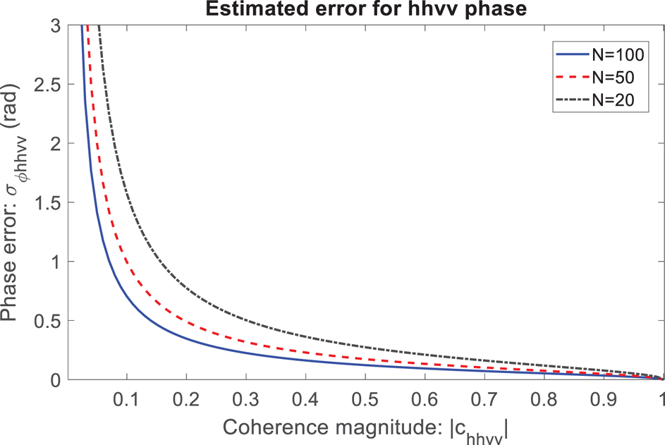
Fig. 4. hhvv phase error as a function of hhvv coherence magnitude and number of range bins, N.
The application of Eqns (3) and (4) to an ice-sheet radar backscatter model (Fujita and others, Reference Fujita, Maeno and Matsuoka2006; Jordan and others, Reference Jordan, Schroeder, Castelletti, Li and Dall2019) implicitly assumes that we are considering the received signal phase rather than the de-ramped phase stored by the ApRES, Eqn (2). To assess the impact of de-ramping upon the coherence, we consider a term from the numerator of Eqn (3) which has proportionality

for the de-ramped signal. Using Eqn (2) it follows that

and hence the de-ramped signal has the opposite hhvv phase polarity to the received signal. To correct for this we replace c hhvv with c hhvv* but from herein do not notate this explicitly.
2.3.2. Polarimetric power
The polarimetric phase shift also results in modulation of radar power as a function of azimuthal angle, and past analyses have used this as an indicator of ice fabric anisotropy (Fujita and others, Reference Fujita, Maeno and Matsuoka2006; Matsuoka and others, Reference Matsuoka, Power, Fujita and Raymond2012; Li and others, Reference Li2018). Following Matsuoka and others (Reference Matsuoka, Power, Fujita and Raymond2012) the co-polarized power anomaly can be calculated from the multi-polarization data via
where [P i] is the returned power of the ith bin, [〈P〉] is the mean power (averaged over all polarization planes) and the square bracket dB notation [χ] = 10log 10(χ) is assumed. Equation (8) assumes that all other aspects of the radar power equation (geometric spreading, attenuation loss, volume scattering) are independent of polarization and is typically calculated using a moving average or smoothing function with respect to the depth coordinate.
3. Theoretical Background
To interpret the polarimetric data analysis, we now summarize a formulation that relates ice fabric anisotropy to dielectric anisotropy (Fujita and others, Reference Fujita, Maeno and Matsuoka2006), including an original formulation of dielectric anisotropy in the near-surface (firn) layer. We then outline a commonly used polarimetric matrix backscatter model (Fujita and others, Reference Fujita, Maeno and Matsuoka2006), including its adaptation to model the hhvv coherence phase (Jordan and others, Reference Jordan, Schroeder, Castelletti, Li and Dall2019), and provide an overview of how the model is used to estimate horizontal fabric properties.
3.1. Dielectric model of ice fabric anisotropy
In this study the c-axis orientation distribution of the ice fabric is formulated in terms of a second-order orientation tensor (Woodcock, Reference Woodcock1977; Montagnat and others, Reference Montagnat2014). The tensor eigenvalues describe the relative concentration of c-axes aligned with each principal coordinate direction/eigenvector and have properties: E 1 + E 2 + E 3 = 1 and E 3 > E 2 > E 1 (Fujita and others, Reference Fujita, Maeno and Matsuoka2006). As in previous radar studies (Fujita and others, Reference Fujita, Maeno and Matsuoka2006; Drews and others, Reference Drews2012; Brisbourne and others, Reference Brisbourne2019; Jordan and others, Reference Jordan, Schroeder, Castelletti, Li and Dall2019) we assume that the E 3 eigenvector (the eigenvector corresponding to the E 3 eigenvalue) is vertical, with the E 1 and E 2 eigenvectors in the horizontal plane to be solved for from the data analysis. The E 2 eigenvector represents the direction of greatest horizontal c-axis alignment.
The appendix of Fujita and others (Reference Fujita, Maeno and Matsuoka2006) describes an effective medium model that relates the orientation tensor to the bulk dielectric tensor. This approach is justified as the crystals are ~ mm in size and the radio wavelength is ~ m. This model results in a bulk (macroscopic) birefringence
where ${\Delta \epsilon }'=\lpar \epsilon _{\parallel c}-\epsilon _{\bot c}\rpar$ is the birefringence of an ice crystal with $\epsilon _{\parallel c}$
 and ε⊥c the dielectric permittivities for polarization planes parallel and perpendicular to the c-axis. The horizontal eigenvalue difference, E 2 − E 1, quantifies the horizontal asymmetry of the ice fabric. At ice-penetrating radar frequencies, Δε′ ≈ 0.034 (Fujita and others, Reference Fujita, Matsuoka, Ishida, Matsuoka and Mae2000). Anisotropy in the conductivity of the crystal can be neglected as the bulk conductivity of polar ice is dominated by acidity content (Fujita and others, Reference Fujita, Maeno and Matsuoka2006).
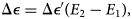
In this study we interpret ice fabric/dielectric anisotropy in the near-surface (firn) which is described by a dielectric mixing model of (anisotropic) ice and (isotropic) air inclusions. In the Appendix we provide a derivation that generalizes the bulk birefringence for solid ice (Eqn (9)) to take into account the ice volume fraction, ν (the single additional variable compared to the solid-ice case). To first order, in terms of a small parameter expansion, this gives a result of the form

where 0 ≤ ν ≤ 1 and f(ν) is a polynomial function of ν. f(ν) is defined on [0,1] and can be interpreted as reduction factor for the birefringence of firn with respect to solid ice (Fig. 5). Due to the unavailability of firn density measurements in our study region (to best of our knowledge the closest example is ~ 250 km upstream (Alley and Bentley, Reference Alley and Bentley1988)) we do not use Eqn (10) explicitly, and instead use the solid-ice version, Eqn (9). However, the Appendix is included for the benefit of future studies where firn density measurements may be available.
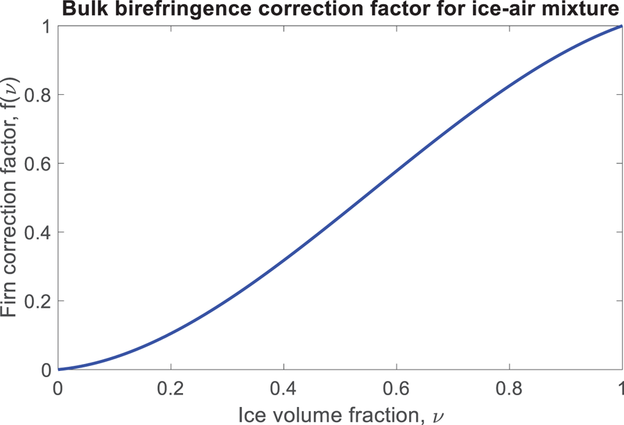
Fig. 5. Reduction factor for the birefringence of firn with respect to solid ice as a function of ice volume fraction, ν.
3.2. Polarimetric backscatter model of an ice sheet
The polarimetric backscatter model is described in detail by Fujita and others (Reference Fujita, Maeno and Matsuoka2006) and considers a nadir sounding geometry where the ice sheet is modeled as a stratified anisotropic medium and radar reflections are assumed to be specular. For the general case, the model incorporates the combined polarimetric effect of birefringent propagation (associated with smoothly varying fabric asymmetry) and anisotropic scattering (associated with local fabric discontinuities). Mathematically the model is formulated as a matrix product and has a functional dependence upon: α (the angle from the E 1 eigenvector to the h polarization, or equivalently, E 2 eigenvector to the v polarization), δ (the polarimetric phase shift along the principal axes) and r (the anisotropic scattering coefficient ratio). The model is defined using Cartesian coordinates with the z-axis vertical and aligned with the E 3 eigenvector.
The backscatter model applies to the full ice column which, in general, contains different layers with varying layer orientation. In this study we are interested in using the model to perform fabric estimates for depth-sections where: (i) there is a suitably high coherence magnitude, (ii) the inferred ice fabric is consistent with a model of unchanging azimuthal orientation within a depth-section.
3.2.1. Using the model to estimate fabric orientation
The prevailing horizontal c-axis (E 2 eigenvector) is estimated by comparing observed azimuthal properties of the vertical phase gradient, dϕhhvv/dz (measured with respect to θ) with modeled (simulated with respect to α). An advantage to using dϕhhvv/dz (instead of ϕhhvv) to infer fabric orientation is that it is not significantly impacted by propagation in anisotropic ice above the layer where fabric is being assessed.
Collating past results from Fujita and others (Reference Fujita, Maeno and Matsuoka2006), Matsuoka and others (Reference Matsuoka, Power, Fujita and Raymond2012), Jordan and others (Reference Jordan, Schroeder, Castelletti, Li and Dall2019), we simulated the azimuth-phase dependence of δ[P] (Fig. 6a) and ϕhhvv (Fig. 6b) and dϕhhvv/dz (Fig. 6c) for fixed bulk birefringence with depth-invariant principal axes and isotropic scattering (r=1).
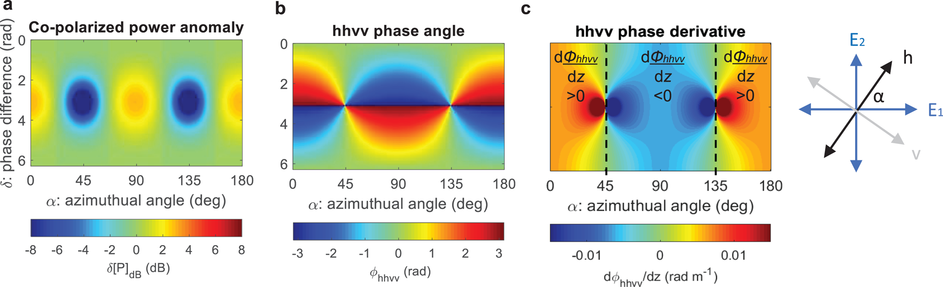
Fig. 6. Simulated dependence of polarimetric power and hhvv coherence phase for radio propagation in a birefringent ice sheet: (a) δ[P], (b) ϕhhvv, (c) dϕhhvv/dz. The definition of the principal angle, α, is shown in relation to the E 2 and E 1 eigenvectors and the h−v measurement system. Panel (a) considers a single set of co-polarized measurements (equivalent to hh) whereas panels (b) and (c) pair hh and vv measurements at 90 degree intervals. The angular dependence of dϕhhvv/dz is used as a diagnostic for fabric orientation, and the ‘90 degree zones’ of positive and negative gradients are marked in panel (c). Following Jordan and others (Reference Jordan, Schroeder, Castelletti, Li and Dall2019) the units in (c) assume a fixed bulk birefringence, Δε = 0.0035.
When the incident polarization planes are aligned with the principal axes (α = 0°, 90°) they continue to propagate in a single polarization state throughout the medium and ϕhhvv is equivalent to δ and

(Jordan and others, Reference Jordan, Schroeder, Castelletti, Li and Dall2019). There is a positive hhvv phase gradient when α = 0° as the v polarization travels at a slower phase velocity than the h polarization (and vice versa when α = 90°). In practice, the orientation of the E 2 and E 1 eigenvectors are most easily inferred by matching the angular transitions between positive and negative phase gradient at α = 45°, α = 135° to the data.
The differing azimuthal symmetry properties for ϕhhvv and δ[P] demonstrate an advantage to using the coherence method to infer fabric orientation. Specifically, dϕhhvv has 180 degree azimuthal symmetry which matches the 180 degree azimuthal symmetry of the orientation tensor. On the other hand, δ[P] has 90 degree azimuthal symmetry. Due to this degeneracy (with respect to the 180 degree symmetry of the orientation tensor) there is therefore an angular ambiguity for the power if the measurement plane is perpendicular or parallel to the E 2 eigenvector.
Model simulations for ϕhhvv and δ[P] for anisotropic scattering (r ≠ 1) can be found in Jordan and others (Reference Jordan, Schroeder, Castelletti, Li and Dall2019), Fujita and others (Reference Fujita, Maeno and Matsuoka2006) and Matsuoka and others (Reference Matsuoka, Power, Fujita and Raymond2012) respectively. For ϕhhvv the central result is that 180 degree azimuthal symmetry is preserved between isotropic and anisotropic scattering, enabling fabric orientation to be determined for different scattering regimes.
3.2.2. Using the model to estimate fabric asymmetry
Equation (11) indicates that E 2 − E 1 (the horizontal eigenvalue difference) is proportional to |dϕhhvv(α = 0°, 90°)/dz|. As f c and c are constants and εice can be approximated as a constant, |dϕhhvv(α = 0°, 90°)/dz| can be used to estimate E 2 − E 1. In Jordan and others (Reference Jordan, Schroeder, Castelletti, Li and Dall2019), low-pass filtering of ϕhhvv was used to evaluate |dϕhhvv/dz| and obtain estimates for E 2 − E 1. However, in this study (due to there being limited regions of high coherence magnitude) we evaluate |dϕhhvv/dz| using a linear approximation across a local depth window.
4. Results
4.1. Polarimetric coherence, power, and depth-range selection
Figure 7 shows the mean (polarization-averaged) power, co-polarized power anomaly, hhvv coherence magnitude and hhvv coherence phase from four example sites along the traverse. Data from the shallowest 500 m of ice was considered, as this marks the approximate depth where returned power was above the noise floor (≈ 80 dB) at all sites. Depth windows of 40 m were used in the coherence estimates corresponding to N = 93 in Eqn (3). In the power plots there are eight independent measurements (due to the 22.5 degree angular resolution) with θ = 0° and θ = 180° identical. In the coherence plots there are four independent estimates (θ = 0, 22.5, 45 and 67.5°), with θ = 90, 112.5, 135, 157.5 and 180° generated by continuing the rotation pattern in Figure 3.
Fig. 7. Polarimetric power and coherence at four sites from the traverse. Far left: Mean (polarization-averaged) power. Center left: co-polarized power anomaly. Center right: hhvv coherence magnitude. Far right: hhvv phase angle. The approximate ice thicknesses are 805 m, 780 m, 760 m, 730 m at sites 2, 6, 7, 8. The pink dashed bounding boxes indicate depth intervals in the near-surface and deeper ice where |c hhvv| is sufficiently high for ice fabric estimates to be made. The angular coordinate, θ, is defined with respect to magnetic north/west (Fig. 2).
The ice fabric estimates were performed over depth intervals where the following three criteria were met. First, when there is relatively high |c hhvv| (an angular average of 0.3 or greater, which is informed by the hhvv phase error relationship in Fig. 4). Second, the azimuthal properties of dϕhhvv/dz conform with the modeled azimuthal symmetry properties of dϕhhvv/dz in Figure 6c (specifically, when there is evidence for ‘90 degree zones’ of positive and negative phase gradient). This step tests if the principal axes can be considered unchanging in the depth interval. Third, the depth interval is sufficiently large to contain at least two separate coherence averaging windows, ensuring that the phase gradient estimates contain at least two independent sample regions.
At Site 2 (broadly representative of sites 1, 5 and 10) there is low |c hhvv| (generally < 0.25) at all depths. Therefore, at these sites ice fabric cannot be estimated at any ice depth. At Site 6 (broadly representative of sites 3, 4, and 9) there is high |c hhvv| (generally > 0.5) at all angles for depths < 50 m and ice fabric was estimated in the near-surface. At sites 7 and 8 there are bands of high |c hhvv| in both the near-surface and deeper ice (≈170–280 m and ≈280–360 m respectively). At these sites we were able to estimate ice fabric in the near-surface and over these limited intervals in deeper ice.
Figure 7 confirms that low |c hhvv| is associated with a randomization of ϕhhvv. By contrast, regions of high |c hhvv| are associated with greater phase continuity and there is evidence for vertical phase shifting in the regions highlighted by the pink bounding boxes in Figure 7. Previous work by Jordan and others (Reference Jordan, Schroeder, Castelletti, Li and Dall2019) demonstrated that a low-power SNR results in low |c hhvv|. However, Figure 7 indicates that the converse is not necessarily true, and a high-power SNR does not guarantee high |c hhvv|. For example, at ice depth z ≈ 100 m the majority of the sites have low |c hhvv| whereas the power is ≈30–40 dB above the noise floor. Suspected polarimetric decorrelation mechanisms include reflections from non-specular layers and reflections from non-parallel layers.
Figure 7 indicates that, at sites 7 and 8, the bands of high |c hhvv| in deeper ice are associated with 180° azimuthal power periodicity, likely due to a dominance of anisotropic scattering (Fujita and others, Reference Fujita, Maeno and Matsuoka2006; Matsuoka and others, Reference Matsuoka, Power, Fujita and Raymond2012). However, at the angular resolution of the measurements (22.5°) it is difficult to separate 90° power periodicity (dominated by birefringent propagation) from 180° power periodicity. Figure 7 also indicates limited evidence for power anisotropy in the near-surface, but we will later show using the coherence method that fabric anisotropy is present.
4.2. Ice fabric estimates
Using the polarimetric coherence method the depth-azimuth properties of dϕhhvv/dz were used to determine horizontal fabric properties. Specifically, the measurement angle (θ) was referenced to the modeled angle (α) by identifying the angular transitions between positive–negative phase gradient (α = 45°) and negative–positive phase gradient (α = 135°) in Figure 6c, thereby enabling the principal axes (α = 0, 90°) to be established. We then estimated horizontal ice fabric asymmetry (the E 2 − E 1 eigenvalue difference) from |dϕhhvv/dz|, Eqn (11).
Figure 8 shows c hhvv and ϕhhvv at sites 7 and 8 over the depth intervals where the fabric estimates were made: the near-surface (defined here as z < 50 m), and deeper ice (170 < z < 280 m at Site 7 and 280 < z < 360 m at Site 8). In deeper ice, at both sites, the sign of dϕhhvv/dz switches from positive to negative between θ = 22.5° and θ = 45°, enabling α = 45° to be estimated as the average between these two values using $\theta \approx {1\over 2} \lpar 22.5+45\rpar ^\circ \approx 34^\circ$ . Subsequently, comparing with the model simulation in Figure 6c, α = 0° was estimated to be θ ≈ (34 + 135) ° ≈ 169° and α = 90° was estimated to be θ ≈ (34 + 45)° ≈ 79°. To estimate fabric asymmetry in deeper ice, we then evaluated |dϕhhvv/dz| for θ = 0, 67.5°, either side of the inferred principal angle of 79° using linear regression applied to Eqn (11). This is indicated by dashed lines in Figure 8 and gives E 2 − E 1 ≈ 0.19 at Site 7 and E 2 − E 1 ≈ 0.21 at Site 8.
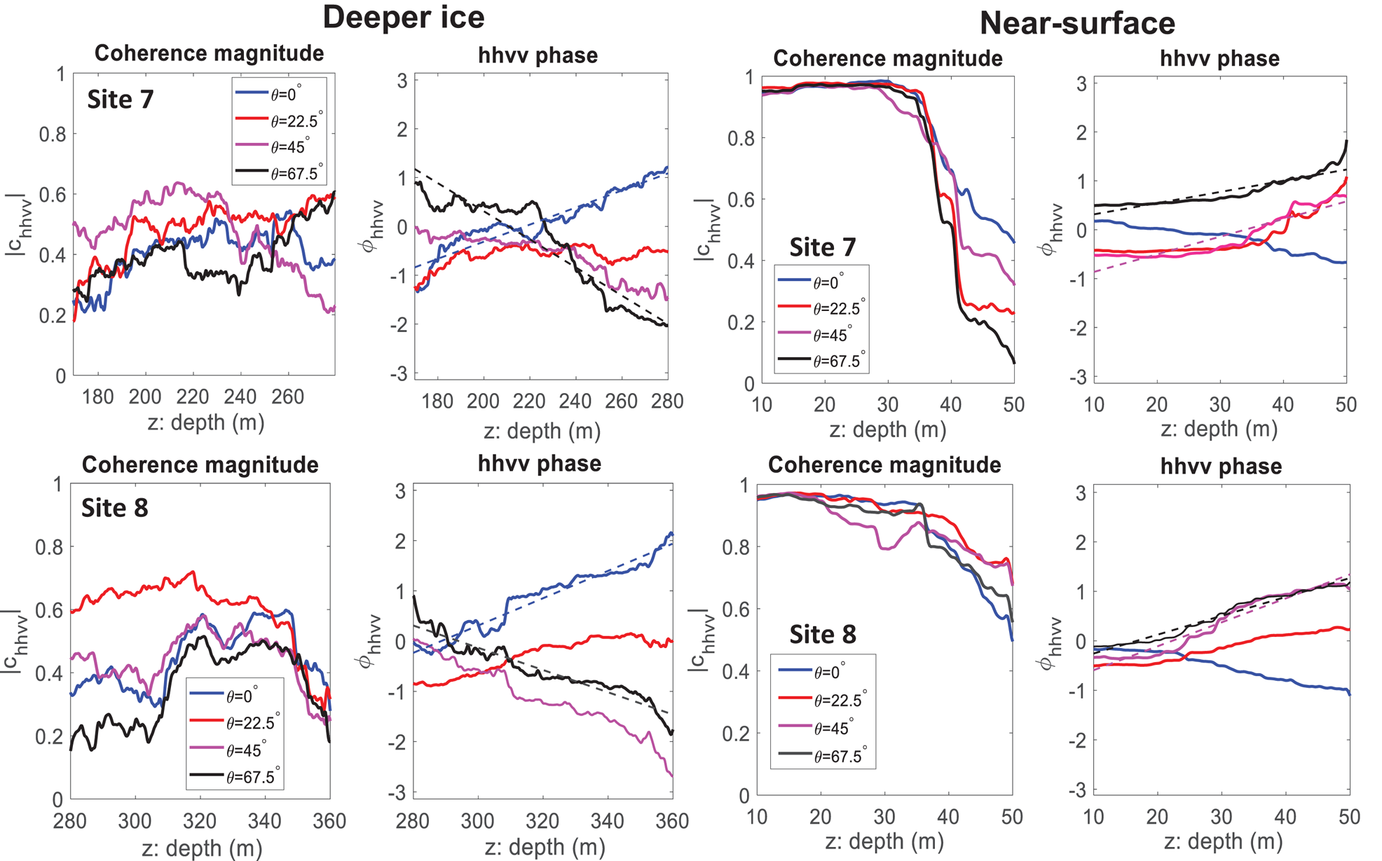
Fig. 8. Ice fabric estimates at sites 7 and 8 using the vertical phase gradient method. The regression lines (angles either side of the inferred principal axis) that are used to estimate the E 2 − E 1 eigenvalue difference are indicated.
The high coherence band in the near-surface persists to a depth z ≈ 50 m. To ensure at least two independent depth regions were included in the fabric estimate the coherence averaging window was reduced to 20 m. Both near-surface plots in Figure 8 indicate that the sign of dϕhhvv/dz switches from negative to positive between θ = 0° and θ = 22.5° enabling α = 135° to be estimated using $\theta \approx {1\over 2}\lpar 0+22.5\rpar ^\circ \approx 11^\circ$ . Hence, comparing with the model simulation in Figure 6c, we can infer that α = 0° is estimated at θ ≈ (11 + 45)° ≈ 56°, and α = 90° is estimated at θ ≈ (11 + 135)° ≈ 146° (45° and 135° correspond to the angular difference between the negative–positive transition in phase gradient and the principal axes). Following the same approach as deeper ice, we then evaluated |dϕhhvv/dz| either side of the inferred principal angles, giving E 2 − E 1 ≈ 0.23 at Site 7 and E 2 − E 1 ≈ 0.46 at Site 8.
Due to only including two independent depth intervals in the coherence estimate (Eqn (3)) we did not propagate the E 2 − E 1 errors from the |dϕhhvv/dz| regression slopes in Figure 8. (Each plot in Fig. 8 shows more than two points because a moving average is used in the coherence estimate.) Additionally, the following sources of bias could effect the estimation of E 2 − E 1. First, the angular uncertainty of the inferred principal angle is ≈ 20° which, following the analysis in Appendix C by Jordan and others (Reference Jordan, Schroeder, Castelletti, Li and Dall2019), could result in estimation biases of up to $\pm \approx 20\percnt$ (positive and negative biases occur dependent upon the value of δ). Second, the transmit–receive antenna separation (≈ 10 m) results in deviations from a vertically propagating wave in the near-surface (e.g. at 30 m depth this angular offset is estimated to be ≈ 5°). This scenario is mathematically equivalent to there being a tilt angle between the E 3 eigenvector and the vertical and a discussion of the estimation bias is provided in Appendix A by Jordan and others (Reference Jordan, Schroeder, Castelletti, Li and Dall2019). Third, from the relationship in Figure 5, it is predicted that a non-zero air volume fraction in the near-surface will lead to a minor underestimation in E 2 − E 1. Despite these limitations, all E 2 − E 1 estimates are physically plausible (in the allowed range 0 < E 2 − E 1 < 0.5 given the constraint E 3 > E 2 > E 1) and yield consistent patterns.
4.3. Ice fabric estimates in relation to ice flow
Figure 9a summarizes ice fabric orientation estimates relative to the direction of ice flow. In the near-surface, the prevailing horizontal c-axis (E 2 eigenvector) is orientated consistently between sites, and is closer to perpendicular to flow. In deeper ice, the prevailing horizontal c-axis is also consistent between sites and aligned closer to parallel to flow. Also shown in Figure 9a are the principal strain-rate directions and relative magnitudes. The Cartesian strain rates were calculated from satellite-derived surface velocity measurements (Rignot and others, Reference Rignot, Mouginot and Scheuchl2011, Reference Rignot, Mouginot and Scheuchl2017), with a Gaussian-kernel, 2D-convolutional derivative with kernel standard deviation of 2 km. Gridded strain rates were then converted to principal strain rate magnitudes and directions through a coordinate transform of the strain rate tensor.
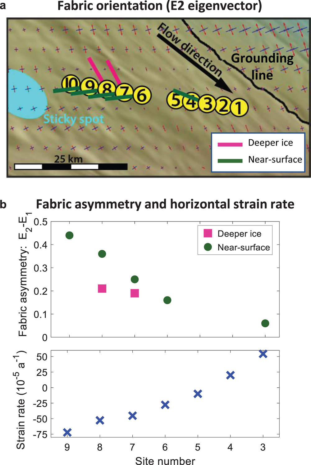
Fig. 9. (a) Summary of the orientation (prevailing horizontal c-axis/E 2 eigenvector) of ice fabric estimates relative to ice motion. The pink and green lines illustrate the direction of the E 2 eigenvector (greatest horizontal c-axis concentration) in the deeper ice and the near-surface. The red and blue crossed arrows indicate the principal strain rate vectors (extension and compression) computed from the ice surface velocity (Rignot and others, Reference Rignot, Mouginot and Scheuchl2011, Reference Rignot, Mouginot and Scheuchl2017). (b) Magnitude of fabric asymmetry (E 2 − E 1 eigenvalue difference) across the survey transect (upper plot) compared with minimum principal horizontal strain rate (lower plot). Negative strain rates correspond to compression.
Figure 9b summarizes the magnitude of the fabric asymmetry (E 2–E 1 eigenvalue difference) across the sites. In the near-surface, the magnitude of fabric asymmetry increases toward the center of Whillans Ice Stream (or, equivalently increases as the measurement sites get closer to the sticky spot). In deeper ice the magnitude of fabric asymmetry is similar at the two sites.
5. Discussion
5.1. Fabric development in ice sheets
To place our Whillans Ice Stream fabric results in context we now summarize fabric development in different stress regimes present in the ice sheets. The structure of a single ice crystal makes deformation along basal planes (perpendicular to the c-axis) over an order of magnitude more favorable, compared to deformation across basal planes (parallel to the c-axis) (Alley, Reference Alley1988; Azuma, Reference Azuma1994). In polycrystalline ice, this result is also true in a statistical sense, where the orientations of individual c-axes modify the effective viscosity of the bulk material. The anisotropic deformation behavior of individual ice crystals results in the c-axes continuously migrating toward the direction of maximum compression, and the fabric developing a preferential orientation.
Preferential fabric orientation has been observed in ice cores at ice domes where the vertical compression of ice causes the c-axes to preferentially align vertically (Gow and Williamson, Reference Gow and Williamson1976; Wang and others, Reference Wang2002). In the limiting case this fabric is referred to a ‘single maximum’ (E 3 ≈ 1, E 2 ≈ E 1 ≈ 0 in terms of the fabric eigenvalues). From Eqn (11) this vertical anisotropy appears as isotropic to radar sounding measurements. In regions where a lateral component of tension is present, such as ice divides or ice rises, the c-axes tend to align in a plane orthogonal to the flow/extension direction (Wang and others, Reference Wang2002; Weikusat and others, Reference Weikusat2017; Brisbourne and others, Reference Brisbourne2019). In the limiting case, this fabric is referred to as a ‘vertical girdle’ ($E_{3}\approx E_{2}\approx {1\over 2}\comma\; E_{1}\approx 0$ in terms of the fabric eigenvalues). From Eqn (11) this horizontal anisotropy can be detected by radar sounding measurements.
In contrast with ice divides and domes there has been more heterogeneity observed in ice fabric that forms in ice streams (Jackson and Kamb, Reference Jackson and Kamb1997; Horgan and others, Reference Horgan, Anandakrishnan, Alley, Burkett and Peters2011; Picotti and others, Reference Picotti, Vuan, Carcione, Horgan and Anandakrishnan2015; Smith and others, Reference Smith2017), illustrating the diversity of stress regimes that can be present. Specifically, ice in fast flow can exhibit the following fabrics:
1. A single maximum. The Whillans Ice Stream trunk was inferred from multi-component seismic data to exhibit a single-maximum fabric in deeper ice, with the near-surface firn layer approximately a random fabric (Picotti and others, Reference Picotti, Vuan, Carcione, Horgan and Anandakrishnan2015). This is consistent with unconfined thinning of Whillans Ice Stream associated with downstream acceleration.
2. A vertical girdle where the prevailing horizontal c-axis is perpendicular to flow. This was inferred from shear wave splitting seismic data at Rutford Ice Stream by Smith and others (Reference Smith2017), and was more precisely referred to as a horizontal partial girdle. It occurs due to the combination of longitudinal extension and lateral confinement.
3. A vertical girdle where the prevailing horizontal c-axis is parallel to flow. This was inferred from active-source seismic data at Thwaites Glacier, West Antarctica by Horgan and others (Reference Horgan, Anandakrishnan, Alley, Burkett and Peters2011). It occurs in regions where englacial deformation is dominated via the interaction with bed topography, in particular upstream features (Picotti and others, Reference Picotti, Vuan, Carcione, Horgan and Anandakrishnan2015).
4. A multiple-maximum fabric perpendicular to the shear plane. This was observed by Jackson and Kamb (Reference Jackson and Kamb1997) from direct samples (300 m deep boreholes) near to the shear margin of Whillans Ice Stream, and results from simple-shear glide with re-crystallization.
5.2. Interpretation of radar fabric measurements within Whillans ice stream
The fabric orientation result for the near-surface in Figure 9a corresponds to the second class of fabric described above (prevailing horizontal c-axis flow-perpendicular). This result is consistent with migration toward the compressive strain rate axis and the orientation of the surface strain components. This result suggests that the near-surface fabric is sensitive to the deformational regime of the surface ice. The fabric orientation result for deeper ice in Figure 9a corresponds to the third fabric type described above (prevailing horizontal c-axis flow-parallel). This result is consistent with englacial ice reacting to longitudinal compression associated with basal resistance from the nearby sticky spot. However, it is not consistent with the surface strain rates (as the compression axis is approximately perpendicular to the horizontal c-axis orientation).
In our radar study we established the presence of greater azimuthal fabric anisotropy (both within the ice column and regarding the development of near-surface anisotropy) than the seismic study of the region by Picotti and others (Reference Picotti, Vuan, Carcione, Horgan and Anandakrishnan2015). However, Picotti and others (Reference Picotti, Vuan, Carcione, Horgan and Anandakrishnan2015) predict that, away from their study region, the c-axes will rotate away from vertical and into the flow direction as longitudinal stresses become more compressive. Specifically, this is expected to occur in the downstream portion of Whillans Ice Stream, where it interacts with discrete sticky spots (Luthra and others, Reference Luthra, Anandakrishnan, Winberry, Alley and Holschuh2016), and the grounding line (Bindschadler and others, Reference Bindschadler, Stephenson, MacAyeal and Shabtaie1987), shown in Figure 1. This places the ice in our study area in a more complex deformation regime than purely longitudinal extension, potentially reconciling our result in deeper ice with Picotti and others (Reference Picotti, Vuan, Carcione, Horgan and Anandakrishnan2015).
The inferred fabric strengths in deeper ice (E 2 − E 1 ≈ 0.2) correspond to a moderately strong vertical girdle fabric (limiting case E 2 − E 1 = 0.5). This azimuthal anisotropy is broadly comparable to the maximum azimuthal anisotropy observed in the Greenland ice cores: NEEM (North Greenland Eemian Ice), GRIP (Greenland Ice Core Project) and NorthGRIP (Montagnat and others, Reference Montagnat2014). The West Antarctic Ice Sheet divide (Kluskiewicz and others, Reference Kluskiewicz2017) and South Pole (Voigt, Reference Voigt2017) Antarctic ice cores both exhibit a stronger maximum azimuthal anisotropy, where E 2 − E 1 is close to the limiting-case of a vertical girdle fabric.
5.3. Radar-derivation of ice fabric and recommendations for future surveys
This study underscores the fact that the polarimetric coherence method is better suited than radar power in estimating spatial variation ice fabric. Specifically, the analyses of radar power do not show clear evidence for near-surface fabric anisotropy and do not provide clear constraints on fabric strength and orientation. The polarimetric coherence magnitude, |c hhvv|, provides a metric to assess where in the ice column fabric can be reliably estimated. We therefore recommend that |c hhvv| should be calculated in the field at the time of polarimetric data acquisition, enabling for a survey site location to be adjusted or for increased stacking to be applied during data acquisition.
As implemented by previous studies (Fujita and others, Reference Fujita, Maeno and Matsuoka2006; Matsuoka and others, Reference Matsuoka, Power, Fujita and Raymond2012) we recommend taking multi-polarization measurements at a slightly higher angular resolution (e.g. 15 degrees) than the 22.5 degrees used in this study. This higher angular resolution will enable more accurate estimates of the fabric orientation and asymmetry (Jordan and others, Reference Jordan, Schroeder, Castelletti, Li and Dall2019). Alternatively, a single set of quad-polarized (fully polarimetric) measurements could be used to reconstruct co-polarized data at a given azimuthal angle and then estimate the fabric as described in this study. This approach would have the advantage of improving the angular accuracy of the fabric orientation estimate but is dependent upon the SNR of the cross-mode terms, s hv, s vh.
Finally, the estimation of horizontal fabric properties using the coherence method compliments seismic methods for characterizing ice fabric, better suited for recovering vertical fabric properties (Picotti and others, Reference Picotti, Vuan, Carcione, Horgan and Anandakrishnan2015; Brisbourne and others, Reference Brisbourne2019). The directional sensitivity of these two classes of geophysical method will potentially enable a complete 3D characterization of ice fabric.
6. Summary and Conclusions
This study adapted a polarimetric coherence method (Dall, Reference Dall2010; Jordan and others, Reference Jordan, Schroeder, Castelletti, Li and Dall2019) to estimate ice fabric using the ApRES. The method was trialed in a fast-flow region of West Antarctic, near to the suture zone of Whillans and Mercer ice streams where a basal sticky spot is present. The method enabled estimation of the prevailing horizontal c-axis (E 2 eigenvector) and magnitude of the horizontal fabric asymmetry (E 2 − E 1 eigenvalue difference). Furthermore, it provided a means to infer spatial patterns in the fabric (both within the ice column and between measurement sites).
In Whillans Ice Stream, the method demonstrated repeatable results in both the near-surface (z < 50 m) and deeper ice (z ≈ 170–360 m), revealing a rotation in the prevailing horizontal c-axis with ice depth and rapid local development of fabric asymmetry in the near-surface. In the near-surface the inferred fabric properties are consistent with the surface compression direction, whereas in deeper ice the inferred fabric properties are consistent with englacial ice reacting to longitudinal compression associated with basal resistance from the nearby sticky spot.
Acknowledgments
TMJ would like to acknowledge support from EU Horizons 2020 grant 747336-BRISRES-H2020-MSCA-IF-2016. DMS would like to acknowledge partial support from an NSF CAREER award. Field data collection was supported by NSF grant ANT-1543441 as part of the SALSA project. We thank Julian Hanna, Sarah Neuhaus, Marino Protti and Aurora Roth for data collection assistant and UNAVCO, Antarctic Support Contract, Kenn Borek Air and the New York Air National Guard for logistic support. We would like to thank Jørgen Dall, Technical University of Denmark, and Carlos Martin and Alex Brisbourne, British Antarctic Survey, for their helpful comments.
Appendix
The effective medium model of fabric anisotropy in the firn layer combines the fabric orientation tensor formulation in the appendix of Fujita and others (Reference Fujita, Maeno and Matsuoka2006) with the Looyenga mixing relations (Looyenga, Reference Looyenga1965) for the two component mixture between ice and air, parameterized by the ice–air volume fraction, ν. The derivation assumes that the air inclusions are isotropic with dimensions much less than the radar wavelength and that dielectric anisotropy arises purely due to the real component of the dielectric permittivity of ice crystal grains.
Following Fujita and others (Reference Fujita, Maeno and Matsuoka2006), the principal permittivities of the ice component can be expressed in terms of the eigenvalues of the orientation tensor as

with the index i = 1, 2, 3. For an ice–air mixture, the Looyenga mixing relations for the effective permittivity are of the form

where the permittivity of air is assumed to be unity. Substituting εii for εeff in Eqn (A2) gives the following formula for the principal, effective, permittivities

We now wish to derive a formula for the bulk birefringence of the ice–air mixture in the horizontal plane $\Delta \epsilon = \epsilon ^{{\rm eff}}_{22}-\epsilon ^{{\rm eff}}_{11}$ . To do this in an analytically tractable way we can rewrite Eqn (A3) in the form

where X i = Δε′E i/ε⊥c is a small parameter ($\approx {1\over 100}$ or less). Following a first-order Taylor expansion of $\lpar 1+X_{i}\rpar ^{ {1} {\scale83% /} {3}}$
 , and then expanding the cubic to first order in X i, we arrive at

Subsequently, upon cancelation of zeroth-order terms when subtracting, the birefringence of the ice–air mixture is given by

where

is a third-order polynomial in ν.


 Open access