


Introduction
The Antarctic subglacial environment is one of the least explored regions on Earth. From the few successful attempts to access this environment, information about its nature has transformed the way we view the continent (Priscu and Christner, Reference Priscu, Christner and Bull2004; Fricker and others, Reference Fricker, Scambos, Bindschadler and Padman2007; Priscu and others, Reference Priscu, Vincent and Laybourn-Parry2008; Siegfried and Fricker, Reference Siegfried and Fricker2018; Venturelli and others, Reference Venturelli2020; Vick-Majors and others, Reference Vick-Majors2020). Reports by international working groups (Priscu and others, Reference Priscu2003; NRC, 2007) concluded that interdisciplinary research on subglacial environments can: (1) reveal the role that subglacial water and saturated sediments play in ice stream dynamics and mass balance, (2) yield novel climatic information contained in lake sediments and the overlying ice sheet and (3) produce new information on the distribution and functioning of biological, chemical and physical systems on our planet. Before 2007, no explicit protocols or standards had been established for environmental stewardship of the subglacial environment, except for general guidelines provided in the Antarctic Treaty System. Once it was realized that subglacial environments harbor active ecosystems (Karl and others, Reference Karl1999; Priscu and others, Reference Priscu1999, Reference Priscu2003), it became clear that direct exploration was required to understand these unique yet numerous systems but environmental stewardship was paramount (NRC, 2007). The 2007 National Research Council (NRC) report presented a series of recommendations for clean access to the subglacial environment and the Scientific Committee on Antarctic Research (SCAR) developed a Code of Conduct for exploration and research of subglacial aquatic environments (SCAR, 2011). Both documents concluded that chemical and biological contaminants in drilling fluids should be documented and clean drilling and sampling technologies should be used as practicable.
Reports have shown that mechanical drilling using hydrocarbon-based drilling fluids can contaminate ice core and subglacial water samples as well as the subglacial environment itself (Christner and others, Reference Christner, Mikucki, Foreman, Denson and Priscu2005; Alekhina and others, Reference Alekhina2007, Reference Alekhina, Ekaykin, Moskvin and Lipenkov2018; Talalay and others, Reference Talalay2014). For this reason, the first clean access to a subglacial lake (Whillans Subglacial Lake, SLW) by the Whillans Ice Stream Subglacial Access Research Drilling (WISSARD) project during the 2012–13 austral summer, used a hot water drill fitted with clean access technology (Priscu and others, Reference Priscu2013; Christner and others, Reference Christner2014; Tulaczyk and others, Reference Tulaczyk2014; Rack, Reference Rack2016). Clean access components of the WISSARD drill consisted of submicron particle filtration and high-intensity UV treatment of drilling water. The potential for contamination during drilling was monitored in real time using a series of sampling ports throughout the system. This allowed potential sources of contamination to be identified before breakthrough, ensured that forward contamination to the subglacial environment was minimized, and verified that samples returned to the surface were not compromised by surface contamination (Priscu and others, Reference Priscu2013; Michaud and others, Reference Michaud2020). The Subglacial Antarctic Lakes Scientific Access (SALSA) project employed all clean access protocols described in these publications and maintained the same physical layout as the WISSARD drill, which has been described previously in detail (Blythe and others, Reference Blythe, Duling and Gibson2014; Burnett and others, Reference Burnett2014; Rack and others, Reference Rack2014).
The SALSA project modified the WISSARD clean access drill by adding additional hose length so that it could create a borehole through the thicker ice and deeper water cavity associated with Mercer Subglacial Lake (SLM), and improved the drilling and reaming approach to ensure that the borehole remained straight, vertical and of even diameter from top to bottom. Specific drilling and operational differences between WISSARD and SALSA include:
• WISSARD drilling speed was ~1 m min−1 (~60 m h−1) relying on a ream while tripping out to widen the borehole to ~0.4 m diameter. The SALSA drilling speed over the entire borehole averaged (±SD) 0.23 ± 0.01 m min−1 (13.80 ± 0.06 m h−1), which eliminated the need for a major ream while tripping out. WISSARD drilling operations also removed the drill from the borehole at ~750 m beneath the ice surface to evaluate the depth and integrity of the borehole before breakthrough. When the drill was redeployed, a bifurcated borehole (that would have compromised scientific tool deployment) developed at ~750 m. About 12 h of additional reaming was required to remove the bifurcation, which reduced the time for science operations.
• WISSARD used multiple nozzles on the drill head: a cone nozzle for firn drilling and a straight jetting nozzle for the ice section of the hole. The SALSA drill used only a 30° solid cone nozzle allowing continuous drilling from the ice surface to the subglacial lake without nozzle changes or reams.
• WISSARD drilling with a straight jetting nozzle made it difficult to enlarge the diameter of the hole at the ice/lake interface, a region critical to the successful retrieval of scientific tools deployed into the lake water cavity. Once the WISSARD straight jetting nozzle broke through the ice/lake interface, the thermal efficiency of the drill head was reduced by the influx of lake water, making it difficult to enlarge this critical portion of the borehole. The 30° solid cone nozzle used by SALSA produced a much larger diameter borehole at the ice/lake interface upon breakthrough.
• The WISSARD drill had 1000 m of drill hose, whereas the SALSA drill had 1400 m of hose to accommodate the thicker ice over SLM.
• The drill tower set up for WISSARD required extending/retracting the tower from over the borehole for scientific tool deployment costing several hours every time the drill tower was moved to accommodate science operations. SALSA combined the drill tower and science towers into one system. The combined system provided a safer system for deck workers and a quicker exchange between the drill and science teams after drilling was completed or a ream was needed, while also assuring that the drill and all tools were centered in the drill hole.
• The return water pump on both the WISSARD and SALSA drilling projects used a Rodriguez Well (Schmitt and Rodriguez, Reference Schmitt and Rodriguez1960) to place the return water pump ~0.8 m from the main drill hole and at a depth below piezometric equilibrium of the lakes. This setup allowed the water level to be pumped down before breakthrough to below the anticipated hydrostatic equilibrium level. After observing rapid freeze-up of borehole water at the air–water interface during WISSARD, SALSA employed an almost continuous hot water back flush to the Rodriguez Well to keep the air–water interface in the borehole from freezing over.
• The SALSA drilling system included more instrumentation to monitor pressure and temperature during drilling:
(i) A pressure sensor on the return water pump (Keller series 33 X) with real-time readout at the surface allowed SALSA drilling operations to determine when breakthrough into the subglacial lake occurred and document that lake water rose upward into the borehole.
(ii) A calibrated load cell on the drill tower sheave produced real-time information at the surface allowing identification of irregularities that occurred during drilling and breakthrough into the lake. Real-time load cell (and hose payout) data were displayed continuously on a large (~40 cm wide × ~20 cm high) digital display at the surface allowing the drilling and science team to follow drilling progress from anywhere on the drilling platform.
(iii) Seabird model 39 temperature–pressure sensors were placed 4 and 200 m above the drill head to collect and store temperature and depth information during drilling.
• The entire WISSARD drill team was new to clean access drilling, although members of the team helped design and build the system. On SALSA, four members of the drill team had prior experience building the drill, drilling two access boreholes with WISSARD, and clean entry into a subglacial water cavity. The team of seven SALSA drillers developed a close synergistic working environment with each other and with the science team.
• Importantly, the science team worked closely with the SALSA drillers on drill deployment allowing for rapid drill setup and integrated input to address challenges that occurred during both drilling and scientific sampling.
In addition to modifications associated with drilling, the scientific objectives of the WISSARD and SALSA projects were distinct. WISSARD sampled SLW and the Whillans Ice Stream grounding zone, focusing on how dynamic glaciological, sedimentological and biogeochemical processes can synergistically stabilize the ice sheet. SALSA sampled SLM, a deeper subglacial lake, focusing on contemporary biodiversity and carbon cycling, and how these are regulated by the remineralization and cycling of relict marine organic matter. Herein, we describe details of the SALSA project's scientific goals, drilling operations, sampling strategy and subglacial tool deployment used to measure subglacial physical, chemical and biological conditions in the water column and sediments. We also examine issues related to fallout of basal ice debris upon breakthrough into the lake water cavity and its implications for potentially modifying the surficial lake sediments that were subsequently sampled by coring.
Study site
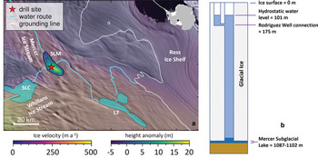
Eight lakes at the downstream confluence of the Mercer and Whillans ice streams fall within three distinct hydrologic basins based on regional bed topography, ice thickness and connected lake events (Fricker and others, Reference Fricker, Scambos, Bindschadler and Padman2007; Carter and others, Reference Carter, Fricker and Siegfried2013; Siegfried and others, Reference Siegfried, Fricker, Carter and Tulaczyk2016): the Southern Basin (including Conway Subglacial Lake (SLC), SLM and Lake 7; Fig. 1a); the Central Basin (including SLW) and the Northern Basin (including Engelhardt Subglacial Lake, SLE). The hydrology of SLM is fed in part (~25%) by water derived from East Antarctica (Carter and Fricker, Reference Carter and Fricker2012), is influenced by drain/fill cycles in a lake immediately upstream (SLC; Siegfried and others, Reference Siegfried, Fricker, Carter and Tulaczyk2016), and lies more than 100 km along its hypothesized water drainage path upstream from the present grounding line of the West Antarctic ice sheet (Carter and others, Reference Carter, Fricker and Siegfried2013). SLM was in a draining phase at the time of sampling (Siegfried and Fricker, Reference Siegfried and Fricker2021).

Fig. 1. (a) Locator map and regional subglacial hydrology of the southern catchment of downstream Mercer and Whillans ice streams. Ice velocity (Mouginot and others, Reference Mouginot, Rignot and Scheuchl2019) overlain on an imagery mosaic (Scambos and others, Reference Scambos, Haran, Fahnestock, Painter and Bohlander2007), with active subglacial lake outlines of SLC, SLM and Lake 7 (L7; Fricker and Scambos, Reference Fricker and Scambos2009). Grounding line (Depoorter and others, Reference Depoorter2013) shown in white and hypothesized subglacial water flow paths (Carter and others, Reference Carter, Fricker and Siegfried2013) shown in cyan. Surface height anomaly over SLM was produced following the methods of Siegfried and others (Reference Siegfried, Fricker, Roberts, Scambos and Tulaczyk2014). The field camp was located within 30 m of the drill hole (both within the boundaries of the star). (b) Vertical aspect of the borehole and lake (drawn to scale) showing the hydrostatic water level in the borehole, the borehole connection to the Rodriguez Well, ice thickness and lake water depth. All measurements are relative to the ice surface.
Based on data collected by the SALSA project the ice overlying the lake at the point of sampling (84.640287° S, 149.501340° W at breakthrough) was shown to be 1087 m thick with a lake water depth of 15 m (Fig. 1b). Ice thickness and water depth were measured using: (1) phase-sensitive radar assuming ice permittivity (ɛ r = 3.18) for the entire column (i.e. no firn correction) yielding an estimated depth of 1088 m in December 2016; (2) load cell changes and the encoder payout readings from a medium duty winch fitted with 3/16 in (4.8 mm) diameter stainless steel wire; (3) changes in vertical profiles of conductivity, temperature and pressure (CTD) measured with a Seabird 19plus V2 SeaCAT profiler that provided high-resolution pressure measurements at 4 scans s−1; (4) video imaging and line payout on a MacArtney CORMAC Q3 series winch fitted with a factory-marked (1 m increment) purposely fabricated, pre-tensioned woven jacket Kevlar/Mylar fiber optic cable (Teledyne Cable Solutions). Although all measurements were in general agreement, we used data from the CTD profiler for all borehole and lake water measurements owing to the robust and accurate nature of this instrument and the potential errors caused by cable stretch and sheave slip associated with wire/cable measurements, particularly at depth. Based on the scan rate and drop speed of the instrument (~30 m min−1), we estimate the depth error associated with the CTD data was ~0.1 m. The Thermodynamic Equation of Seawater 2010 (TEOS-10; McDougall and Barker, Reference McDougall and Barker2011) was used to obtain all derived CTD data at the latitude of collection (e.g. depth, specific conductance and freezing temperature), using absolute salinity derived from conductivity following the limnological application of Pawlowicz and Feistel (Reference Pawlowicz and Feistel2012). The final depth of the air–water interface after breakthrough was measured using payout increments marked on the fiber cable on the MacArtney winch with attached clump weight cameras to visualize the interface (Burnett and others, Reference Burnett, Rack, Zook and Schmidt2015).
SALSA hypotheses and objectives
SALSA is an interdisciplinary subglacial project that interweaves discovery with hypothesis-driven research to address how subglacial hydrology and relict deposits of marine organic carbon regulate microbial ecosystem processes in a hydraulically active subglacial environment. The overarching hypothesis of the SALSA project is: contemporary biodiversity and carbon cycling in hydrologically active subglacial environments associated with the Mercer and Whillans ice streams are regulated by the mineralization and cycling of relict marine organic matter and through interactions among ice, rock, water and sediments. This hypothesis was addressed through an integrated study of subglacial hydrology, the character of water column and sedimentary organic carbon, geobiological processes and paleobiological contributions to sediments in SLM. The SALSA study addresses key questions directly relevant to West Antarctica's ice-sheet stability, subglacial hydrological system and the deep-cold subglacial biosphere.
A conceptual diagram showing the subglacial hydrology of the region and biogeochemical pathways investigated by the SALSA project is presented in Fig. 2a. This figure shows a cut-away of the region depicting relict organic material deposited during past marine incursions, its role in driving carbon cycling in the subglacial lake sediments and water column, the export of organic carbon and nutrients to the sea via encasement in basal ice during basal freeze-on and through subglacial water flow, and the role of bacterial carbon cycling, driven by compounds derived from the breakdown of organic matter and by mineral weathering. Figure 2b shows the intricate linkages between ice, rock, sediment (including recycled marine and terrestrial microfossils) and subglacial water, and their relationships with carbon cycling pathways. Implicit in both panels of Fig. 2 is the overarching role that ice-sheet history has on contemporary microbial carbon transformations. This diagram also indicates the key importance of subglacial water in providing the microbes and medium for biological reactions, as a source for sediment suspension and transport, and its role in ice-sheet dynamics. The overarching SALSA hypothesis was addressed by collecting surface geophysical measurements in concert with a suite of in situ water column measurements and geobiological data obtained on samples returned to the surface.
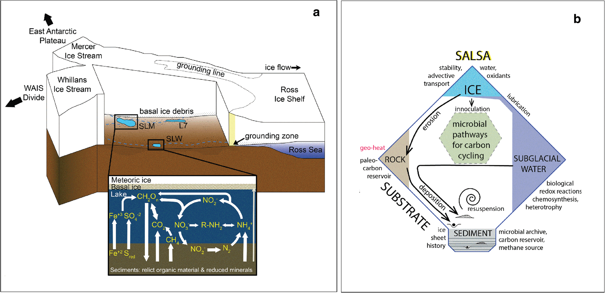
Fig. 2. (a) Schematic showing the locations of SLM and SLW relative to the Mercer and Whillans ice streams and the grounding zone (after Venturelli and others, Reference Venturelli2020). The inset presents contemporary and relict biogeochemical process thought to occur in the study lakes. (b) Conceptual diagram showing how ice, water, rock and sediment are linked to numerous dynamic process and ultimately microbial carbon cycling (center of the diagram) the latter of which forms the basis for the scientifically integrated SALSA project. Both panels reveal the integrated nature of the SALSA program and the requirement to include scientists with diverse backgrounds who are willing to work synergistically to address the common theme of subglacial carbon cycling.
Drilling operations
Before drilling began in December 2018, much of the equipment (drill, science laboratories and operations structures) and fuel had been staged at Camp 20 (along the South Pole Overland Traverse [SPOT] route) the previous season and was traversed the final ~150 km from Camp 20 to SLM during the drilling season. Materials not staged at Camp 20 during the previous season were traversed ~900 km from McMurdo Station to SLM in November and early December of the drilling season.
One of the first tasks at SLM was to groom a skiway that allowed LC130 and smaller ski-equipped aircraft to operate. Scientists and operations staff (~50 total personnel) were brought to the field in these aircraft to set-up the drilling system and science labs. Once camp and drill set-up were complete, a 175 m deep (~0.4 m diameter) Rodriguez Well was drilled (see Fig. 1b). A water return pump for the drilling system was placed near the bottom of the Rodriguez Well so that its inlet was 171 m below the ice surface (4 m above the floor of the Rodriguez Well). The return pump had a Keller Series 33X pressure sensor mounted to the return water hose ~4 m above the return pump inlet (167 m below the ice surface; 8 m above the floor of the Rodriguez Well). The pressure sensor was placed 4 m above the return pump to minimize interference from the electromagnetic field generated by the pump motor and to avoid potential reduction in static pressure caused by pumping. The depths of the Rodriguez Well and return water pump and pressure sensor were selected to ensure that they would remain below the hydrostatic level of the water in the borehole that was pumped down to minimize introduction of drill water into the lake water cavity at breakthrough.
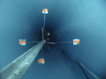
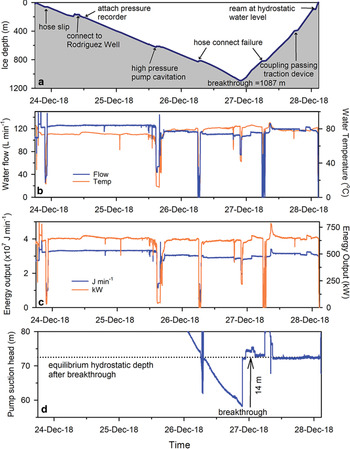
Drilling of the main borehole began at 17:45 on 23 December 2018 (NZDT, New Zealand daylight time) and was offset from the Rodriguez Well by ~0.8 m. During initial stages of drilling the main borehole, a melt connection was made near the bottom of the Rodriguez Well, allowing water between the main borehole and the Rodriguez Well to exchange freely (Fig. 3). Lake breakthrough occurred at 21:40 NZDT on 26 December 2018, 1087 m beneath the ice surface. The drilling rate averaged (±SD) 0.23 ± 0.01 m min−1 (13.80 ± 0.06 m h−1) over the entire range of borehole drilling. Following breakthrough, the borehole was upward reamed at an average (±SD) rate of 0.61 ± 0.08 m min−1 (36.6 ± 4.8 m h−1) during return of the drill hose and drill-head to the surface. The temporal drilling profile, average flow rate, drill water temperature and energy (heat) output from the production plant (not at the drill head) are shown in Fig. 4. The flow rate, drill water temperature and heat output were relatively constant at 114 ± 20 L min−1, 74.9 ± 11.2°C and 3.65 × 10⁷ ± 0.77 × 10⁷ J min−1 (608.3 ± 128.3 kW), respectively. Irregularities noted in the drilling and reaming rates in Fig. 4a were related to: (1) hose slippage caused by guiding sheave joint slip on the drill tower; (2) cavitation associated with a faulty primer pump supplying feed water to the high pressure pump, which was replaced; (3) a reduction in drilling speed required for the passage of hose couplers through the hose traction device and (4) a hose connection failure when a barb fitting came loose on the low pressure feed from the water tank. These drill protocols produced a ~0.4 m diameter borehole through 1087 m of ice. The diameter of the entire borehole was visually verified by observing the clearance of horizontally fixed metal rods (‘whiskers’) of a known diameter (0.4 m) with cameras attached to the Deep SCINI clump weight (see also Fig. 3). The clump weight stabilizes the section of the Deep SCINI remotely operated vehicle (ROV) that extends upward to the surface to stabilize the tether. The Deep SCINI ROV is then attached to the clump weight on a much shorter tether allowing it to operate without the drag of the entire cable. The Deep SCINI clump weight was fitted with cameras and lights and was often used independently from the ROV to observe the borehole, lake water and benthic sediments.

Fig. 3. Borehole image showing the 0.4 m diameter ‘whiskers’ (tabs with orange marking) used to determine borehole diameter and the connection to the Rodriguez Well (lower right) containing the return pump (the hose and power cord for the return pump are visible in the Rodriguez Well). The whiskers were mounted on a rod beneath the clump weight, the latter of which included a downward facing camera and lights.
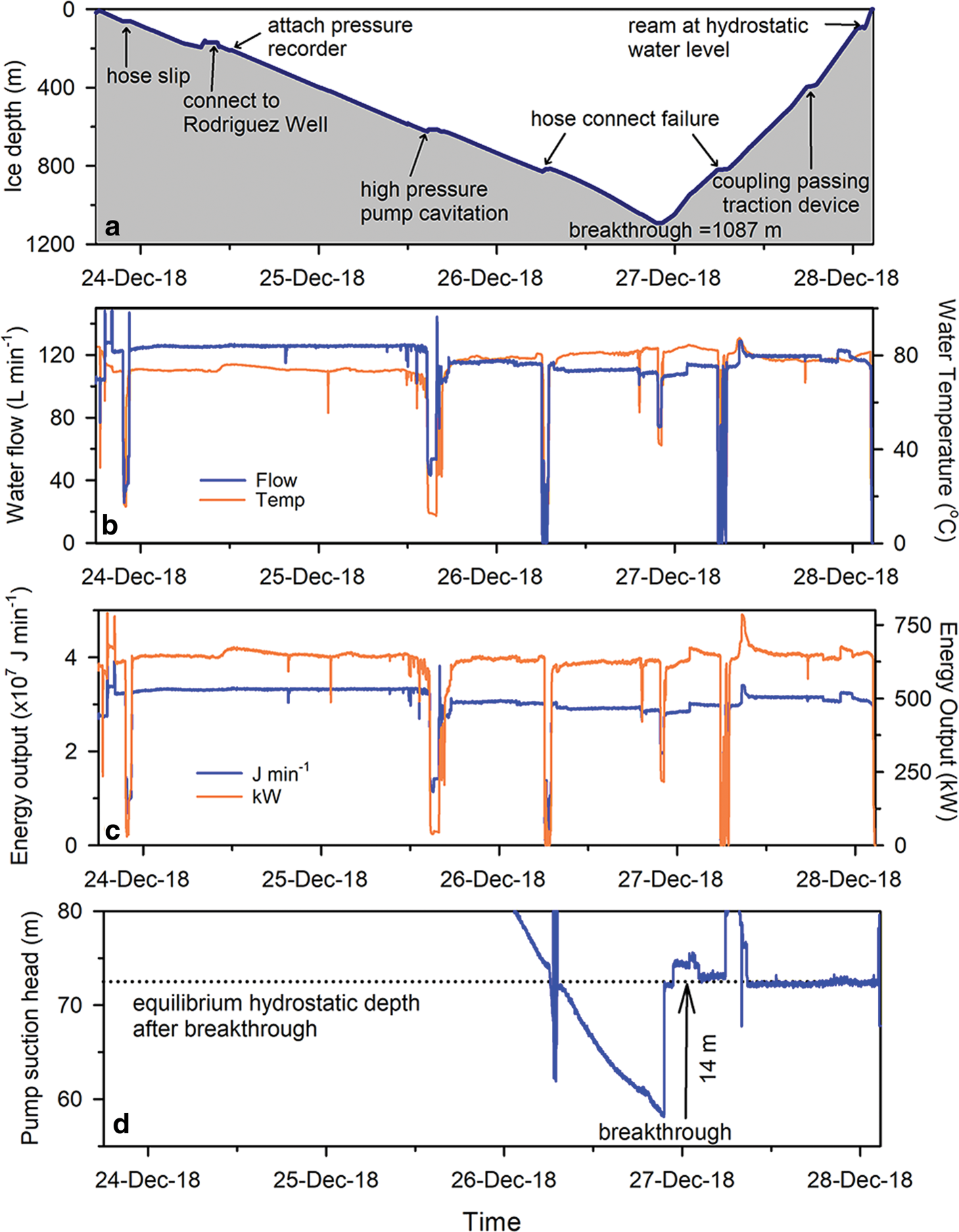
Fig. 4. Parameters associated with initial drilling and reaming operations: (a) drilling progress over time and depth (depicted by the top of the shaded area) and associated deviations during drilling; (b) water flow and drilling water temperature at the drill production plant; (c) heat output from the production plant and (d) change in hydrostatic water level (pump suction) in the Rodriguez Well at breakthrough. The x-axis represents NZDT.
Borehole observations at breakthrough
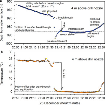
Following breakthrough, the suction head showed a 14 m rise in the Rodriguez Well water (Fig. 4d), which is in hydrostatic equilibrium with the borehole water, as lake water entered the lower borehole following breakthrough. This resulted in a constant hydrostatic level in the borehole of 101 m beneath the ice surface (see also Fig. 1b). The Seabird model 39plus (SBE39) pressure and temperature sensor mounted 4 m above the drill head showed details of depth relative to the hydrostatic water level in the borehole and temperature over the drilling period (Fig. 5). Seabird electronics reported temperature and pressure accuracy and resolution of ±0.002 and 0.0001°C, and ±0.1 and 0.002% of full scale, respectively, for the SBE39.
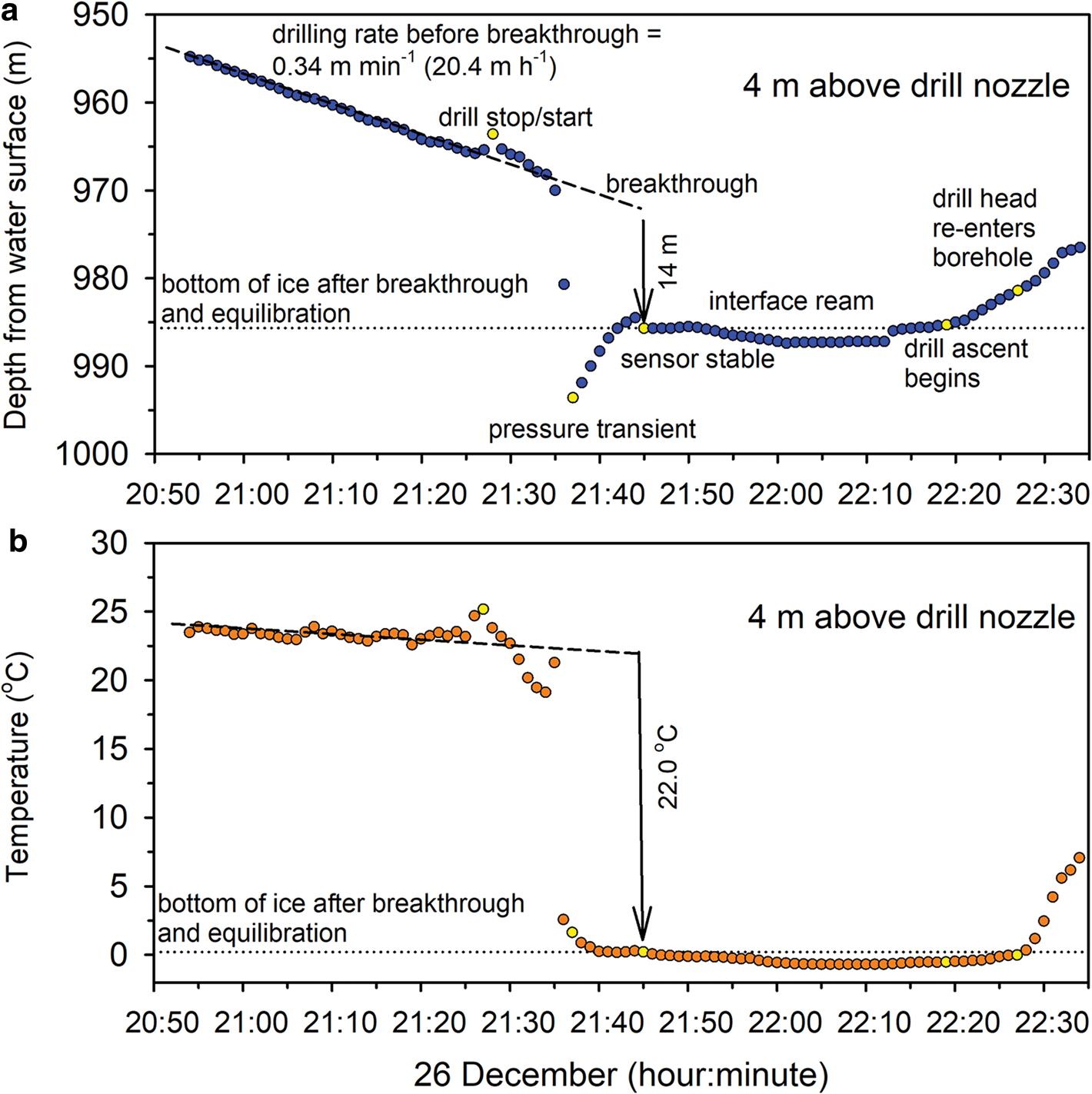
Fig. 5. Detailed vertical and temporal measurements during breakthrough: (a) depth from the borehole water surface (hydrostatic or pressure depth) and (b) temperature measured with a SBE39 sonde mounted ~4 m above the drill nozzle. Yellow circles depict specific events noted by the text in the figure panels. The x-axis represents NZDT.
Lacking simultaneous conductivity information, pressure data from the SBE39 sensors were converted to depth using a linear fit to the depth–pressure relationship determined using TEOS-10 derivations from previous Seabird 19plus V2 SeaCAT profiles; this approach yielded an observed error of no more than ±0.6 m down the entire length of the water column.
Depth data from the SBE39 are shown relative to the depth from the air–water interface in the borehole to reflect the actual water pressure (converted to depth and referred to here as pressure or hydrostatic depth) at the sensor head, allowing comparison to the suction head depth in the Rodriguez Well (Fig. 4d). The sequence of events shown by the data in Fig. 5 is:
• Steady drilling at 0.34 m min−1 (20.4 m h−1) until 21:25 NZDT (~30 min before breakthrough), which is faster than the average drilling rate for the entire borehole of ~0.23 m min−1 (13.80 m h−1).
• Between 21:25 and 21:28 NZDT, a load cell change occurred as the drill was stopped, checked and restarted, as noted in Driller Log 21:30 entry. Drilling resumed by 21:29 NZDT.
• Between 21:34 and 21:35 NZDT, the drill head reached the ice–lake water interface at a hydrostatic depth of 968 m, opening the connection. Lake water rose rapidly up the borehole reaching a transient hydrostatic depth peak of 993.6 m within 3 min.
• The hydrostatic depth transient, possibly enhanced by an effect of the rapid decrease in temperature on the pressure sensor itself, decayed and by 21:45 NZDT the reading stabilized at 985.7 m. The hydrostatic depth increased in depth by 17.5 m from its position at breakthrough. However, based on drilling rate, the drill continued downward ~3.5 m during this time, so the actual change in hydrostatic depth is 14 m (17.5 − 3.5 = 14 m), exactly as recorded by the Rodriguez Well pressure sensor (see Fig. 4d).
• The time period 21:42 to 22:18 NZDT constitutes a ~36 min ‘ream’ of the opening. Based on the continued downward lowering of the drill following breakthrough, much of the ream occurred ~ 3 m below the ice–lake water interface. Because the drill head was below this interface, little change in temperature at the level of the SBE39 (located ~0.5 m above the interface) occurred, and the ream likely did little to widen the opening. This is presumably the reason why a second ream was required after the first Niskin bottle casts were difficult to retrieve through the ice–water interface (see instrument deployment timeline below).
• At 22:19 NZDT, the drill began to ascend slowly. The drill head did not re-enter the borehole until 22:27 NZDT, after which time borehole water temperatures measured by the SBE39 began to rise again.
The following breakthrough model conservation equations were used to estimate the height that lake water rose in the borehole.
Conservation of volume:

where V lb is the volume of the lower portion of the borehole into which the lake water rose at breakthrough; V ub is the volume of the upper portion of the borehole into which meltwater rose at breakthrough and V RW is the volume of the upper portion of the Rodriguez Well into which meltwater rose at breakthrough. Equation (1) ignores the negligible impact of water compressibility on the results.
Conservation of specific conductance (SC):

where V lb is the volume of the lower portion of the borehole into which the lake water rose at breakthrough; V int is the volume of the section of the borehole over which SC was integrated (in our case contains the noted conductivity peaks 1 and 2 in Fig. 6); SCint is the integrated mean SC of the portion of the borehole over which SC was integrated (CTD peaks 1 and 2; 752–1045 m); SCM is the SC of clean meltwater (determined from borehole measurements made well above the observed SC peaks) and SCL is the SC of SLM lake water. Specific conductance at 25°C is used here, rather than in situ conductivity, because it is a nearly perfectly conservative parameter in these dilute aqueous solutions and will be directly comparable to laboratory measurements made on lake water and sediment porewater samples collected.

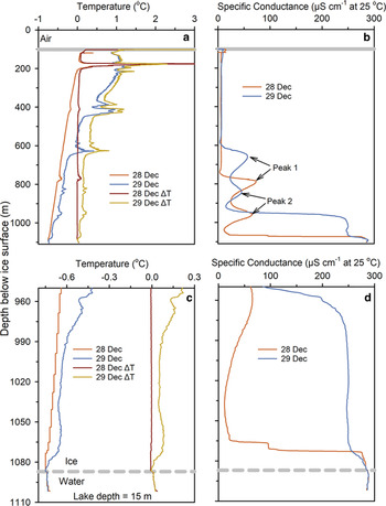
Fig. 6. (a–d) Profiles of temperature, specific conductance and the difference between in situ temperature and freezing temperature ΔT. Panels (c) and (d) include an expanded depth scale below 950 m to highlight details within this region. Specific conductance and ΔT were computed using the thermodynamic equations of seawater 2010 (TEOS-10) using the modifications of Pawlowicz and Feistel (Reference Pawlowicz and Feistel2012) for low salinity water.
Assuming that Rodriguez Well and upper borehole diameters were each 0.4 m, V lb values computed with Eqns (1 and 2) are 28 and 35 m, respectively. The height discrepancy between the V lb values is 7 m (35 − 28 m). The fact that the V lb value computed from SC is larger than that from volume conservation indicates excess SC not attributable to the lake water that entered the borehole upon breakthrough. The excess SC was potentially introduced from melt of debris-rich basal ice.
Physical and chemical characteristics of the borehole following breakthrough
Borehole water temperature profiles made on 28 December, 37 h after breakthrough (~8 h after completion of the upward ream) showed a borehole temperature average (±SD) of −0.32 (0.36)°C (Table 1). Exceptions are peaks at the air–water interface (101 m below the ice surface), and at 175 and 770 m below the ice surface (Fig. 6a). The peak at the air–water interface is the result of extended heat input in this region of the borehole to enlarge the diameter at this interface (see also Tulaczyk and others, Reference Tulaczyk2014), whereas the peak at 175 m coincides with the connection of the borehole with the Rodriguez Well (Fig. 4a). The small peak at 770 m coincides with the hose connection failures when drilling stopped and restarted (Fig. 4a). Lake water temperature was relatively consistent over the 15 m lake water cavity averaging (±SD) −0.74 (0.01)°C. Freezing temperature in the borehole and lake water, computed using TEOS-10 were within 0.05 and 0.02°C, respectively, of the freezing point (Figs 6a, c; Table 1). It should be noted that all borehole temperature and conductance data were obtained with a sonde lowered through the center of the borehole and may not reflect exact conditions at the borehole wall as shown by Talalay and others (Reference Talalay2019) in controlled laboratory experiments with artificial ice. Conditions within the SALSA borehole wall were dynamic and influenced by numerous variables such as ice debris, conductivity gradients, borehole diameter and mixing within the borehole water. These variables change with reaming and small-scale mixing induced by tool deployment. Determining borehole wall conditions and refreezing rates throughout the SLM borehole over time is beyond the objectives of our manuscript.
Table 1. Temperature (°C), specific conductance (SC, μS cm−1 at 25°C), difference between in situ temperature and freezing temperature (ΔT, °C) in the borehole and lake water and the central depth and maximum SC for peaks 1 and 2 shown in Fig. 6b

All data from CTD profiles made on 28 December and 29 December. Positive values of ΔT indicate excess heat above the freezing point. Data were derived from CTD profiles using limnological application of the thermodynamic equation of seawater 2020 (TEOS-10) (Pawlowicz and Feistel, Reference Pawlowicz and Feistel2012). SDs are given in parentheses.
The borehole temperature profile made late on 29 December, 75 h after breakthrough and immediately following a borehole ream, still showed the vertical anomalies observed in the 28 December profile with an additional peak at 626 m. The average (±SD) temperature in the borehole on 29 December was 0.12 (0.63)°C, which was 0.44°C warmer than the average for the 28 December profile (Figs 6a, c; Table 1), reflecting the additional heat added to the borehole following the ream. This additional heat raised the difference between in situ temperature and freezing temperature (ΔT in Figs 6a, c; Table 1) from 0.05 to 0.49°C, inducing melt throughout the borehole. The changes in borehole temperature and ΔT between the 28 December and 29 December CTD profiles were statistically significant (P < 0.001, t-test). Lake water temperature did not change significantly (P = 0.41, t-test) between 28 December and 29 December remaining relatively constant at −0.74 (0.01)°C and within 0.02°C of the freezing point.
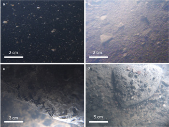
The very small difference in ΔT at the depth of the ice–water interface indicates a dynamic balance between the lake water and overlying ice where small changes in ice density, ice thickness, ice temperature and lake water temperature can result in the formation (accretion) or loss (melting) of ice above the lake. Images of the bottom of the ice sheet (Fig. 7) revealed a ~6 m thick layer of sediment-laden basal ice with an estimated volumetric sediment content of ~20%, which presumably accreted on the bottom of the ice upstream of the lake. Similar basal ice debris layers were observed in the neighboring Kamb Ice Stream (Christoffersen and others, Reference Christoffersen, Tulaczyk and Behar2010; Engelhardt and Kamb, Reference Engelhardt and Kamb2013). Figure 7 also shows the ice–lake water interface with newly accreted ice (Fig. 7c) and sediment clasts on the lake bottom (Fig. 7d). The presence of accretion ice at the SLM ice–water interface indicates active accretion while or before we sampled the lake, which could influence lake water column concentrations of dissolved ions, gases and particulate matter (e.g. Santibáñez and others, Reference Santibáñez2019).

Fig. 7. Images of the lower ~6 m of basal ice taken with side facing cameras mounted on the clump weight showing: (a) dispersed facies of debris-laden basal ice; (b) massive facies of debris-laden basal ice; and (c) the ice–lake water interface showing clear accreted ice in the upper right and lake water in lower left. A downward facing camera was used to image surface lake sediments showing larger clasts that presumably fell from the basal ice upon breakthrough (d).
Specific conductance in the borehole water on 28 December and 29 December was significantly different (P < 0.001, t-test), averaging (±SD) 20.9 (37.0) and 49.3 (79.7) μS cm−1, respectively, whereas the SC in the lake water was constant (average for both dates = 287.2 μS cm−1) (P = 0.89, t-test).
Two distinct peaks in SC were present below 600 m in both the 28 and 29 December profiles (Figs 6b, d). These peaks were centered at 786.3 and 958.9 m in the 28 December profile and were displaced upward by 126.6 and 119.1 m in the borehole to 659.7 and 839.8 m, respectively, in the 29 December profile (Table 1). A distinct step in SC was centered at 1068 m on 28 December with a value of ~96 μS cm−1. SC increased sharply below the step, approaching lake water SC levels. The step was no longer present on 29 December following borehole reaming but was replaced by a dispersed region of elevated SC from 960 to 1073 m. This increase in SC is associated with warmer borehole water temperatures reflecting hot water input from the 29 December ream together with the introduction of upward displaced lake water resulting from differences between return pump and drilling flow rates. The source of the solutes causing the observed vertical changes in SC is most likely from upward-rising lake water and salts associated with basal ice debris. As shown by the height discrepancy of 7 m between the V lb values calculated using conservation of volume and SC relationships, the amount of dissolved solids present in peaks 1 and 2 combined is in excess of the amount that can be attributed to the upwardly displaced initial plug of lake water. These results indicate an additional source of salts to the borehole water, which likely originated from debris-rich basal ice melt.
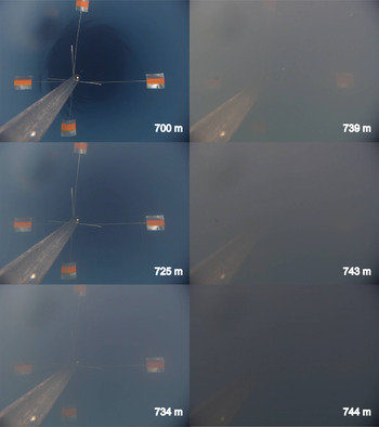
Published data have shown that melted debris-rich ice often has high solute concentrations that are typically orders of magnitude greater than meteoric ice (e.g. Montross and others, Reference Montross2014). Unfortunately, the SALSA project did not collect discrete ice cores that could be used to examine the particulate and geochemical nature of the basal ice. Images of borehole water taken with the clump weight camera on 28 December immediately following breakthrough (Fig. 8) showed a distinct increase in turbidity associated with SC peak 1 in Fig. 6b. The transition from clear to highly turbid water occurred over the depth interval 700–744 m. The borehole remained turbid from a depth of 744 m down to the base of the borehole (data not shown). The most likely source for the suspended sediments is the fine-grained material that was added to the base of the borehole water column with the melting of the debris rich basal ice (Fig. 7) and was drawn up into the borehole by the drilling and reaming operations.
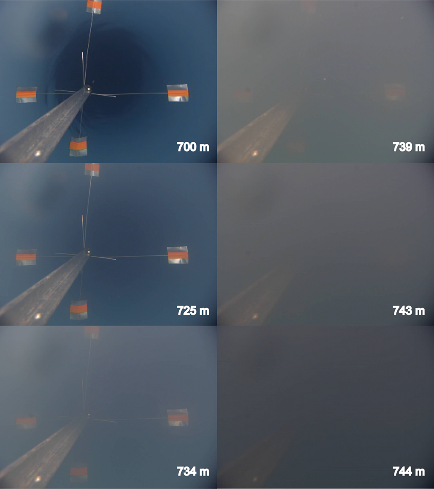
Fig. 8. Images of the water filled borehole from the downward looking camera on the clump weight on 28 December 2019 showing the transition from clear water to highly obscured over the depth interval 700–744 m. Each ‘whisker’, with an orange target is ~20 cm long. Note the significant obscuration below 739 m, which corresponds to the increase in specific conductivity in peak 1 from the 28 December 2019 profile (Fig. 6b).
The bifurcated peaks (peaks 1 and 2) in SC in the lower borehole (Fig. 6b) presumably result from mixing instabilities within the borehole (e.g. Diment, Reference Diment1967) that were caused by the upward ream to the surface on 28 December and the 29 December ream (made before the 29 December CTD profile). The ream that occurred between CTD casts likely displaced water near the bottom of the borehole that contained lake water and suspended basal ice debris, moving peaks 1 and 2 further up the borehole and broadening them as they were diluted by mixing with the drill water and melting of the borehole sidewalls (Table 1).
Borehole tool deployment
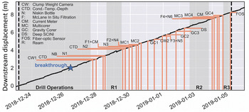
After breakthrough, SALSA science operations occurred over the next ~10 days with three reams to maintain borehole access. Reams 1, 2 and 3 (Fig. 9) lasted 24.9, 28.8 and 10.4 h, respectively. Visual observation of borehole diameter, ice thickness and lake water depth were made using video cameras mounted to the Deep SCINI clump weight (Burnett and others, Reference Burnett, Rack, Zook and Schmidt2015). Following these visual observations initial conductivity, temperature and depth measurements in the borehole and lake water columns were obtained with the Seabird CTD profiler. Additional tools were then lowered into the lake following a planned schedule and sequence that minimized contamination of lake water with sediments mobilized by coring (Table 2; Fig. 9). Four cycles of round-the-clock science operations resulted in the collection of: (1) borehole imagery; (2) two CTD casts, (3) 60 L of lake water plus 10 L of deep borehole water; (4) concentrated particulates >0.2 μm in diameter from in situ filtration of ~100 L of lake water; (5) 10 multicores 0.32–0.49 m long; (6) two gravity cores 1.0 and 1.76 m long and (7) discrete depth current meter measurements that were logged on 30 December at 1 min intervals at mid-depth (7 m) over a 2.4 h deployment, and on 4 January at 6.4, 10.4 and 14.4 m from the ice–lake water surface (8.6, 4.6 and 0.6 m from the bottom of the lake, respectively) at 1 min intervals over a 0.25 h deployment at each depth. Collectively, results from these measurements and analyses of samples will be reported in subsequent manuscripts that characterize the physical and geochemical nature of the water and sediments and to determine the biological structure and functioning of the SLM ecosystem.

Fig. 9. Borehole tool deployment relative to ice motion over the sampling period (NZDT). Ice movement was obtained from a continuous Global Navigation Satellite System located 420 m from the borehole location and processed with precise point positioning methods following Siegfried and others (Reference Siegfried, Fricker, Carter and Tulaczyk2016). See Table 2 for additional information on tool deployment and notation used.
Table 2. Borehole tools deployed over the ~10-day sampling period in SLM
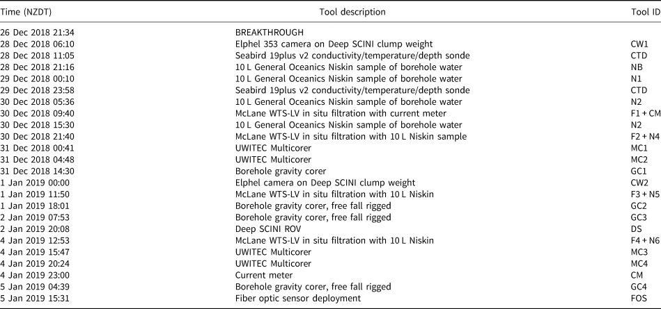
Tool background: CW has been described previously (Burnett and others, Reference Burnett, Rack, Zook and Schmidt2015) and was fitted with Elphel 353 cameras in custom pressure housings. It was lowered on a MacArtney CORMAC Q3 winch fitted with a Teledyne Solutions pre-tensioned woven jacket Kevlar/Mylar fiber optic cable; borehole bulk water sampler is a General Oceanic's Niskin, Model 1010; McLane WTS-LV is a large volume in situ filtration unit modified to fit the minimum borehole diameter of 30 cm (McLane Research Laboratories) has a 142 mm filter holder that accepts filters in series for size fractionation of particulates (Morrison and others, Reference Morrison, Billings and Doherty2000); UWITEC multicorer is described in Hodgson and others (Reference Hodgson2015); borehole gravity corer is a modularly weighted (up to 862 kg) coring device specially fabricated to collect 11.1 cm diameter sediment cores up to 4.6 m long; fiber optic sensor was a multimode optical fiber that functions as a distributed temperature sensor to measure cm-scale vertical profiles of temperature in SLM for one year. A Nortek Aquadopp (#AQD 62490) current meter was used for discrete depth measurements.
The Mercer Ice Stream overlying SLM flows toward the Ross Ice Shelf at a rate of ~0.64 m d−1 based on data from a surface Global Navigation Satellite System station. Consequently, the borehole advected 5.5 m downstream over the course of the science operations period (Fig. 9). The resulting transect is particularly relevant for sediment core collection because the borehole moved progressively farther downstream from the breakthrough location, allowing sequential cores to be collected from essentially undisturbed sediments and reducing the level of potential sediment contamination by basal ice sediment fallout during breakthrough and reaming procedures (discussed in detail later). Despite the flow of the ice stream overlying SLM, we observed no deformation of the borehole with depth over the sampling period. The ice overlying SLM is at the confluence of the Mercer and Whillans ice streams, a region characterized by very low driving stress. Thus, motion is dominated by basal sliding rather than internal deformation. Whillans Ice Stream, in fact, is highlighted in Cuffey and Paterson (Reference Cuffey and Paterson2010) as the only glacier with a ratio of basal velocity to total velocity of 1. The SLM borehole site was also located in the center of a subglacial lake (many ice thicknesses from the nearest shoreline), where the lake water cannot support friction to drive large differences between surface and basal velocity.
Evaluating potential impact of sediment fallout to surface lake sediments
Images collected by cameras during Deep SCINI clump weight deployments revealed sediment laden basal ice, indicating that sediment release into the lake following drill breakthrough and subsequent reams had occurred (Figs 7, 8). Sediment fall-out from basal ice has the greatest potential to affect the multicoring operations that focused on collecting the upper ~0.5 m of lake sediment, including a preserved sediment/water interface. Geochemical properties and biological activity within the surficial sediments of SLW were inferred to have a large role in carbon cycling in both the lake water and the sediments (e.g. Michaud and others, Reference Michaud2016, Reference Michaud2017), prompting our evaluation herein of sediment fallout from basal ice on surficial sediment sampling in SLM. We evaluated the potential impact of sediment fallout using estimates of basal ice sediment volume and fallout characteristics.
Sediment load contained within the basal ice was estimated using brightness thresholds (method adapted from Christoffersen and others, Reference Christoffersen, Tulaczyk and Behar2010) and the sequence (~6 m-thick) was comprised of a dispersed facies (~5 m-thick) containing ~1.4% sediment by volume (Fig. 7a), and a massive facies (~1 m-thick) containing ~17.5% sediment by volume (Fig. 7b). Results from the brightness thresholds estimate that 0.03 and 0.01 m3 of sediment were contained within the ice of the ~0.4 m diameter borehole and in the ice after reaming the borehole (which was ~0.3 m in diameter before the ream) to its original ~0.4 m diameter, respectively. We recognize that a proportion of the borehole closure from 0.4 to 0.3 m diameter following drilling will likely be through freeze-on of borehole water, which may have lower sediment concentrations than the basal ice. However, because the proportion of sediment in the ice removed by reaming is unknown, our calculations assume uniform delivery of sediment load to the lake and that borehole closure results from ice deformation. Grain size analysis of surface sediments collected from SLM were used to constrain particle size distribution of sediment in the accreted basal ice and showed that ~60% of the sediment was <0.063 mm in diameter, which is similar to previously recovered tills from this region (Tulaczyk and others, Reference Tulaczyk, Kamb, Scherer and Engelhardt1998; Hodson and others, Reference Hodson, Powell, Brachfeld, Tulaczyk and Scherer2016).
Sediment settling velocities were calculated as a function of grain diameter, following the equation given by Ferguson and Church (Reference Ferguson and Church2004):

where w is the particle sediment settling velocity, R is the particle's submerged specific gravity (1.65), g is the acceleration due to gravity (9.8 m s−2), D is its diameter, v is the dynamic viscosity of the fluid (1.787 × 10⁻⁶ Pa s for fresh water at 0°C) and parameters C 1 and C 2 are constant values of 18 and 0.4, respectively. Based on computed settling velocities, fine particles of diameter <0.063 mm would require several hours to days to settle through a 15 m deep water column, while grains >0.125 mm would settle within minutes. We assumed that the fine particle sediment fraction (silt and clay) melted out from the basal ice and was transported downstream beyond the sediment core collection sites. Unfortunately, currents at discrete depth within the lake were near the noise floor of the Nortek Aquadopp current meter of ~ 1 cm s−1. This noise floor is based on typical open water marine measurements and is dependent on deployment and environmental conditions (personal communication from B. Huber of Lamont-Doherty Earth Observatory). Given the low beam amplitude during our survey and our deployment technique (the instrument was not moored but rather suspended from a wire line that did not constrain spinning of the meter on its central axis), the noise floor may be higher in our measurements of the SLM water column. Because the lake was in a draining phase during our study, it is likely that there was downstream flow at velocities near or below the noise floor of the current meter. Consequently, our modeling analysis was limited to the coarser sediment fractions, sand-sized and greater (>0.063 mm diameter). Calculated coarse sediment fraction volumes from drilling and reaming of the borehole used in our sediment accumulation analysis were 0.012 and 0.005 m3, respectively.
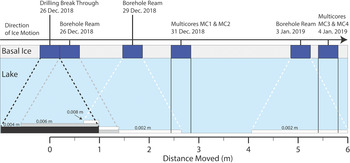
Modeled sediment accumulation thicknesses associated with drilling and reaming operations are shown relative to the locations of multicoring to evaluate the potential impact of these operations on the ensuing sediment core collection (Fig. 10). The general conclusion from model results is that the estimated sediment accumulation at the UWITEC multicore sites (MC1/MC2 and MC3/MC4) from drilling and reaming operations would be at most 0.002 m, which will have a minimal effect on stratigraphy or biogeochemical analysis.

Fig. 10. Sediment accumulation thicknesses (m) associated with drilling (black horizontal bar in lower left) and three reaming events (gray/white horizontal bars along the bottom of the figure) relative to the first and second sets of multicores, MC1 and MC2; 31 December 2018 and MC3 and MC4; 4 January 2019, respectively. Distance moved (m) represents ice movement relative to the initial location of the borehole on breakthrough into the lake. Modeled accumulation from drilling breakthrough on 26 December 2018 was 0.004 m (black horizontal bar), from borehole reaming on 26 December 2018 was 0.002 m (gray horizontal bars), and from borehole reaming on 29 December 2018 and 3 January 2019 was 0.002 m (white horizontal bars). Accumulation thicknesses are based on a 3° angle of sediment dispersion through the water column from the base of the borehole as indicated by dashed diagonal lines with colors corresponding to drilling and reaming events. The length of the large dark blue bars depicted in the basal ice layer represent the borehole location during breakthrough, reaming and coring operations; borehole diameter was assumed to be 0.4 m. The solid vertical lines under the multicore collection dates indicate sediment area sampled by the multicores. Note the lake and ice depth are not to scale. Times represent NZDT.
Conclusions
The SALSA access borehole was drilled through the Mercer Ice Stream (1087 m thick) and entered the 15 m deep water column of SLM in late December 2018. The primary objective of the SALSA project was to examine the role of subglacial water, ice, sediment, rock and paleoclimate on microbial carbon cycling within the water column and sediments of SLM. SALSA drilling operations were modified from the WISSARD project to reduce the time between drilling and science tool deployment, to increase safety of all personnel and to ensure a vertical borehole of uniform diameter. Deployment of pressure and temperature sensors on the drilling system produced a novel and important set of physical and chemical data following breakthrough into the lake and consequent reams of the borehole that should be considered when designing and operating future hot water drills, particularly those requiring clean subglacial access. Future efforts should be made to increase the portability of clean-access hot water drills by reducing their size and mass, thus allowing multiple holes to be drilled during a single season for relatively shallow (i.e. <1500 m) drilling sites such as ice streams and ice shelves. The knowledge gained from such efforts will be key for developing environmentally clean drilling strategies of sufficient capability to enter the subglacial water cavities that lie beneath almost 4 km of ice (e.g. Vostok Subglacial Lake).
Acknowledgements
This material is based upon work supported by the US National Science Foundation, Section for Antarctic Sciences, Antarctic Integrated System Science program as part of the interdisciplinary (Subglacial Antarctic Lakes Scientific Access (SALSA): Integrated study of carbon cycling in hydrologically-active subglacial environments) project (NSF-OPP 1543537, 1543396, 1543405, 1543453 and 1543441). Ok-Sun Kim was funded by the Korean Polar Research Institute. We are particularly thankful to the SALSA traverse personnel for crucial technical and logistical support. The United States Antarctic Program enabled our fieldwork; the New York Air National Guard and Kenn Borek Air provided air support; UNAVCO provided geodetic instrument support. Hot water drilling activities, including repair and upgrade modifications of the WISSARD hot water drill system, for the SALSA project were supported by a subaward from the Ice Drilling Program of Dartmouth College (NSF-PLR 1327315) to the University of Nebraska-Lincoln. J. Lawrence assisted with manuscript preparation. Finally, we are grateful to C. Dean, the SALSA Project Manager, and R. Ricards, SALSA Project Coordinator at McMurdo Station, for their organizational skills, and B. Huber of Lamont-Doherty Earth Observatory for providing the SBE39 PT sensors and the Nortek Aquadopp current meter and assisting with interpretation of the data. B. Huber also provided helpful input on programing and calibrating the SBE19PlusV2 6112 CTD. The manuscript benefited from comments made by K. Makinson, P. Talalay and three anonymous reviewers.


 Open access