


1. Introduction
Long-term care (LTC) costs have shown a significant increase over the recent decades. In the US, data by the National Health Expenditures Account (NHEA) show that expenditures in the Medicare program, aiming to support US residents with low income in LTC, raised from $225 billion in 2000 (2.2% of the gross domestic product (GDP)) to $830 billion in 2020 (3.6% of GDP). Also governmental spending in home health care raised from $32 billion in 2000 to $124 billion in 2020. A similar observation is made in Europe, for instance in Belgium, where LTC spending (in terms of GDP) increased from 1.7% in 2000 to 2.4% in 2019 (source: Eurostat).
The increasing trend of LTC costs is projected to continue in the future (Shi and Zhang, Reference Shi and Zhang2013). According to United Nations projections, the number of elderly people, that is older than 65, is projected to triple from 2020 to 2080 to reach 2.2 billion. The global share of the elderly population is expected to rise from 9.4% in 2020 to 20.6% in 2080, while the demand for LTC services in the years to come is expected to further increase.
Specific insurance products are dealing with LTC risk, notably the classical LTC cover, which provides benefits in case of dependency, and the enhanced pension or life-care annuity. The latter combines regular payments of a life annuity with LTC insurance (see for example, Denuit et al., Reference Denuit, Lucas and Pitacco2019 for more details). In terms of risk management, the pooling of competing risks, that is longevity and morbidity, is quite advantageous as the two risks act in opposite directions (Murtaugh et al., Reference Murtaugh, Spillman, W and arshawsky2001). When moving into dependency, individuals receive higher benefits but also suffer from a decrease in their life expectancy, creating a natural hedge. The key advantages of the life-care annuity relative to the stand-alone products life annuity and classical LTC cover are its potential to decrease the costs and to make coverage available to more potential purchasers (Spillman et al., Reference Spillman, Murtaugh and Warshawsky2003). One reason for this is a reduction in adverse selection. Individuals with low longevity expectations are less likely to buy annuities, forcing insurance providers to increase their premiums accordingly. Indeed, it has been estimated that around 10% of the cost of life annuity premiums is due to adverse selection (Friedman and Warshawsky, Reference Friedman and Warshawsky1990). On the other hand, classical LTC covers are not available to everyone as underwriting mostly rejects people in bad health. Combining both products makes insurance affordable for people in a poor health state for whom it is currently unattractive to buy a life annuity and unaffordable to buy a classical LTC cover. A life-care annuity allows the inclusion of this currently rejected population, which lowers the cost for all and reduces adverse selection (Brown and Warshawsky, Reference Chen, Hieber and Klein2013).
However, estimating the risks of a classical LTC cover or a life-care annuity is a challenging task for the insurance provider, resulting typically in high risk and administration charges. This might explain why the volume of the private market for LTC insurance is still relatively small. Indeed, when looking at the written gross premiums for long-term care insurance (LTCI), it is clear that the private LTC insurance market is limited in most OECD countries, although the need for a market is clearly strong (OECD, 2020). That is the reason why, in this article, we suggest a mutual risk sharing scheme that keeps the advantages of a life-care annuity but shifts risks from the insurance provider to a policyholder pool. As the insurance provider is merely administrative in such a product, we expect lower risk and administration charges at the expense of a higher risk exposure to the policyholders. A mutual insurance product would not guarantee a precise level of retirement income. On top of the investment returns from funded assets, survivors receive a higher payout funded by the “mortality credits” of deceased members. The very first such products are (original) tontines dating back to the 17th and 18th century in Europe (for more details, we refer to Milevsky, Reference Milevsky2015; Li and Rothschild, Reference Li and Rothschild2019). Today, modern versions of these original tontines exist, for example the TIAA-CREF retirement fund in the USA, the Lifetimeplus solution of Mercer in Australia, or “Le Conservateur” in France. In the literature, these modern versions are named pooled annuities, group self annuitization schemes (see, e.g., Piggott et al., Reference Piggott, Valdez and Detzel2005; Valdez et al., Reference Valdez, Piggott and Wang2006; Stamos, Reference Stamos2008; Qiao and Sherris, Reference Qiao and Sherris2013; Donnelly et al., Reference Donnelly, Guillén and Nielsen2013; Donnelly et al., Reference Donnelly, Guillén and Nielsen2014) or (modern) tontines (see, e.g., Sabin, Reference Sabin2010; Forman and Sabin, Reference Forman and Sabin2015; Milevsky and Salisbury, Reference Milevsky and Salisbury2015; Forman and Sabin, Reference Forman and Sabin2016; Fullmer and Sabin, Reference Fullmer and Sabin2018; Li and Rothschild, Reference Li and Rothschild2019; Chen et al., Reference Chen, Fuino, Sehner and Wagner2021). These articles follow a long tradition of mutual with profits products where mortality or investment surplus is shared through an appropriate bonus distribution (see, for example, the well-cited book by Fisher and Young, Reference Fisher and Young1965). While the mentioned literature solely deals with the sharing of mortality risks, we introduce a modern “life-care tontine”, which in addition to retirement income targets the needs of LTC coverage for an ageing population. We introduce the concept of “morbidity credits” that allow to share LTC risks within the policyholder pool. We take advantage of the natural hedge between mortality and morbidity risks and assign people moving to dependency a higher death probability, allowing them to get a bigger share in future mortality credits redistributed among the survivors of the tontine pool. To make the product attractive for subscribers with different risk, we suggest a fairness condition that ensures that the payments are actuarially fair in each payment period (see also Donnelly et al., Reference Donnelly, Guillén and Nielsen2013; Donnelly et al., Reference Donnelly, Guillén and Nielsen2014). In other words, the life-care tontine stays fully funded at all times with each individual investment balance reflecting actual market values. We also allow to pool individuals from different age cohorts (see also Donnelly et al., Reference Donnelly, Guillén and Nielsen2014; Milevsky and Salisbury, Reference Milevsky and Salisbury2016; Denuit, Reference Denuit2019). Such a product design has many advantages. (1) Compared to a life-care annuity, a life-care tontine has significantly lower solvency capital requirement (see also Shao et al., 2015; Chen et al., Reference Chen, Hieber and Klein2019), inducing lower costs. (2) Compared to a classical tontine or pooled annuity, a life-care tontine is also attractive for people in poor health, reducing adverse selection costs (see also, e.g., Valdez et al., Reference Valdez, Piggott and Wang2006 for supporting arguments with respect to mutual insurance schemes and adverse selection). A life-care tontine covers the increasing need of LTC coverage in an ageing society. (3) Being actuarially fair in each payment period, the life-care tontine avoids the disadvantage of a closed tontine pool (see, for example, the discussion in Chen et al., Reference Chen, Hieber and Klein2019). The design allows to keep the pool size at a constant high level, replacing deceased individuals by new members. The sharing within the tontine pool is carried out by the concept of mortality and morbidity credits. (4) Compared to a closed, homogeneous insurance pool, pooling heterogeneous risks, that is different age-cohorts or active/dependent states, allows to increase tontine pool sizes and thus to reduce the overall risk.
In an environment where insurance providers are no longer willing to take on long-term guarantees, one has to avoid that longevity and LTC risks remain fully uninsured. To avoid insurance gaps, it is necessary to design new products adapting to these circumstances. The trend to move to mutual insurance schemes is not restricted to private insurance – it is also manifested in the move from defined benefit to (collective) defined contribution in occupational and state pensions. The presented idea of a mutual risk sharing scheme of mortality and morbidity risk can also help to design occupational pension systems where the insurance provider is either unable or not willing to take the pension’s long-term risks. Adjusting the benefits of pensions by risk factors like autonomy/dependence can further enhance the fairness of the pension system (see also Holzmann et al., Reference Holzmann, Alonso-Garcia, Labit-Hardy and Villegas2019 for a discussion of other risk factors).
The paper is organized as follows: In Section 2, we introduce a 2-state alive/dead framework through a fair tontine scheme allowing members to freely join the pool. This framework enables to pool heterogeneous cohorts, like in Donnelly et al. (Reference Donnelly, Guillén and Nielsen2014), Milevsky and Salisbury (Reference Milevsky and Salisbury2016) and Denuit (Reference Denuit2019). Section 3 extends this to a 3-state framework, with a dependent state getting a specific (higher) payoff. The classical life-care annuity is compared with our life-care tontine. The fairness of the product is demonstrated and the payoffs are smoothed over time to fit the actual needs. Sections 4 and 5 conclude and make additional remarks.
2. 2-state framework
In a first step, we consider a 2-state framework where individuals have two possible states “alive” or “dead”. We later extend this basic setting to a modern life-care tontine. Let us introduce the set of all individuals at initiation by
 $\mathcal{L}_0=\{1,2,...,n\}$
. Time is discretized in periods
$\mathcal{L}_0=\{1,2,...,n\}$
. Time is discretized in periods
 $t=0,1,2,\ldots$
. Assume that individual
$t=0,1,2,\ldots$
. Assume that individual
 $j \in \mathcal{L}_0$
, aged
$j \in \mathcal{L}_0$
, aged
 $x_j$
with a remaining lifetime
$x_j$
with a remaining lifetime
 $T_j$
, contributes a single premium
$T_j$
, contributes a single premium
 $c_j(0)$
at time 0. Financial assets are invested in a risk-free bank account with a time-dependent, deterministic, risk-free rate
$c_j(0)$
at time 0. Financial assets are invested in a risk-free bank account with a time-dependent, deterministic, risk-free rate
 $\delta_s$
,
$\delta_s$
,
 $s\ge 0$
. The maximal age is denoted by
$s\ge 0$
. The maximal age is denoted by
 $\omega$
. For now, the remaining lifetimes
$\omega$
. For now, the remaining lifetimes
 $T_{j}, j \in \mathcal{L}_0$
, are assumed to be independent.
$T_{j}, j \in \mathcal{L}_0$
, are assumed to be independent.
2.A. Tontine payoff
The n individuals form a tontine pool. Given the total initial premium payment, they decide on a withdrawal plan for the pool, that is for
 $t=0,1,2,\ldots$
, they (together) withdraw the amount
$t=0,1,2,\ldots$
, they (together) withdraw the amount
 $W_j(t)$
in a way that the premium equivalence
$W_j(t)$
in a way that the premium equivalence
 \begin{align}\underbrace{\sum_{j=1}^n c_j(0)}_{\text{total contributions}} = \sum_{j=1}^n \underbrace{\sum_{t=1}^{\omega-x_j} e^{-\int_0^t \delta_s \textrm{d}s} W_j(t)}_{\text{discounted benefits individual j}}\,\end{align}
holds. The account value left according to the agreed decumulation plan for individual j at time
 $t=0,1,2...$
is denoted
$t=0,1,2...$
is denoted
 $c_j(t)$
. Equation (2.1) shows the main property of a tontine: the sum of all payoffs to the pool is deterministic, leaving no risk for the insurance provider. The payoff to a single individual
$c_j(t)$
. Equation (2.1) shows the main property of a tontine: the sum of all payoffs to the pool is deterministic, leaving no risk for the insurance provider. The payoff to a single individual
 $W_j(t)$
, however, is random and may depend on the mortality experience in the pool. In the remainder of this section, we will demonstrate that (2.1) holds also at later points in time, that is the tontine scheme is fully funded at all times and satisfies for all
$W_j(t)$
, however, is random and may depend on the mortality experience in the pool. In the remainder of this section, we will demonstrate that (2.1) holds also at later points in time, that is the tontine scheme is fully funded at all times and satisfies for all
 $t\ge 0$
:
$t\ge 0$
:
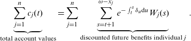 \begin{align}\underbrace{\sum_{j=1}^n c_j(t)}_{\text{total account values}} = \sum_{j=1}^n \underbrace{\sum_{s=t+1}^{\omega-x_j} e^{-\int_t^{s} \delta_u \textrm{d}u} W_j(s)}_{\text{discounted future benefits individual j}}\,.\end{align}
We proceed by iteration to obtain
 $\mathcal{L}_t=\{\,j \in \mathcal{L}_0 \,|\, T_j>t\}$
, the subset of participants still alive at time t. Let us define
$\mathcal{L}_t=\{\,j \in \mathcal{L}_0 \,|\, T_j>t\}$
, the subset of participants still alive at time t. Let us define
 $\mathcal{D}_t=\{\,j \in \mathcal{L}_0 \,|\, t-1<T:j \leq t\} = \mathcal{L}_{t-1} -\mathcal{L}_{t}$
, the subset of participants dying in
$\mathcal{D}_t=\{\,j \in \mathcal{L}_0 \,|\, t-1<T:j \leq t\} = \mathcal{L}_{t-1} -\mathcal{L}_{t}$
, the subset of participants dying in
 $(t-1,t]$
. We denote by
$(t-1,t]$
. We denote by
 ${}_tp_{x_j} = \mathbb{E}[\unicode[Times]{x1D7D9}_{T_{j}>t}]= \mathbb{E}[\unicode[Times]{x1D7D9}_{j \in \mathcal{L}_t}]$
the probability for individual j aged
${}_tp_{x_j} = \mathbb{E}[\unicode[Times]{x1D7D9}_{T_{j}>t}]= \mathbb{E}[\unicode[Times]{x1D7D9}_{j \in \mathcal{L}_t}]$
the probability for individual j aged
 $x_j$
to survive t years and set
$x_j$
to survive t years and set
 ${}_tq_{x_j} \;:\!=\; 1- {}_tp_{x_j}$
. For annual survival and death probabilities, we abbreviate
${}_tq_{x_j} \;:\!=\; 1- {}_tp_{x_j}$
. For annual survival and death probabilities, we abbreviate
 $p_{x_j} \;:\!=\; {}_1p_{x_j}$
and
$p_{x_j} \;:\!=\; {}_1p_{x_j}$
and
 $q_{x_j} \;:\!=\; {}_1q_{x_j}$
. For
$q_{x_j} \;:\!=\; {}_1q_{x_j}$
. For
 $t =1,2,\ldots,\omega-x_j$
, we obtain the Bernoulli distribution
$t =1,2,\ldots,\omega-x_j$
, we obtain the Bernoulli distribution
 $\unicode[Times]{x1D7D9}_{j \in \mathcal{L}_t} \sim \operatorname{Ber}({}_tp_{x_j})$
and
$\unicode[Times]{x1D7D9}_{j \in \mathcal{L}_t} \sim \operatorname{Ber}({}_tp_{x_j})$
and
 $ \unicode[Times]{x1D7D9}_{j \in \mathcal{D}_t } \,|\,\{\, j \in \mathcal{L}_{t-1} \} \sim \operatorname{Ber}(q_{x_j+t-1})$
. Note that our assumption of a maximal age
$ \unicode[Times]{x1D7D9}_{j \in \mathcal{D}_t } \,|\,\{\, j \in \mathcal{L}_{t-1} \} \sim \operatorname{Ber}(q_{x_j+t-1})$
. Note that our assumption of a maximal age
 $\omega$
implies that individuals never reach age
$\omega$
implies that individuals never reach age
 $\omega+1$
, that is
$\omega+1$
, that is
 $q_\omega= 1$
.
$q_\omega= 1$
.
Let us now look at an individual
 $j \in \mathcal{L}_{t-1}$
and a single time period
$j \in \mathcal{L}_{t-1}$
and a single time period
 $(t-1,t]$
. During the time period
$(t-1,t]$
. During the time period
 $(t-1,t]$
, the individual j’s account value accrues to an amount of
$(t-1,t]$
, the individual j’s account value accrues to an amount of
 $e^{\int_{t-1}^t \delta_s \textrm{d}s} c_j(t-1)$
. In case of death in
$e^{\int_{t-1}^t \delta_s \textrm{d}s} c_j(t-1)$
. In case of death in
 $(t-1,t]$
, this account value is lost and distributed to the pool of individuals. Otherwise, the individual receives a payment at time t. This payment is decomposed into a fixed withdrawal
$(t-1,t]$
, this account value is lost and distributed to the pool of individuals. Otherwise, the individual receives a payment at time t. This payment is decomposed into a fixed withdrawal
 $s_j(t)$
and mortality credits from deceased pool members. In Section 3.3, this payoff is extended to a life-care tontine that also includes “morbidity credits”. Each individual’s account value is iteratively determined via
$s_j(t)$
and mortality credits from deceased pool members. In Section 3.3, this payoff is extended to a life-care tontine that also includes “morbidity credits”. Each individual’s account value is iteratively determined via
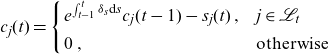 \begin{align}c_j(t) = \left\{ \begin{array}{l@{\quad}l} e^{\int_{t-1}^t \delta_s \textrm{d}s} c_j(t-1) - s_j(t)\,, & j \in \mathcal{L}_{t} \\[5pt]0\,, & \textrm{otherwise}\,\end{array}\right.\end{align}
in a way that the account is depleted at the maximal age
 $\omega$
, that is
$\omega$
, that is
 $c_j(\omega-x_j)=0$
. With this, we can solve (2.3) to get, for individual
$c_j(\omega-x_j)=0$
. With this, we can solve (2.3) to get, for individual
 $j\in \mathcal{L}_{t}$
at time t:
$j\in \mathcal{L}_{t}$
at time t:
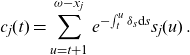 \begin{align}c_j(t) = \sum_{u=t+1}^{\omega-x_j} e^{-\!\int_t^u \delta_s\textrm{d}s } s_j(u)\,.\end{align}
To define the variable part of the payoff (the mortality credits), formally, denote as
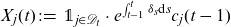 \begin{align*}X_j(t) \;:\!=\; \unicode[Times]{x1D7D9}_{j \in \mathcal{D}_t} \cdot e^{\int_{t-1}^t \delta_s \textrm{d}s} c_j(t-1)\end{align*}
the random variable that is 0 in the case where the individual is alive at time t and equal to the accrued account value
 $e^{\int_{t-1}^t \delta_s \textrm{d}s} c_j(t-1)$
in case of death in the time interval
$e^{\int_{t-1}^t \delta_s \textrm{d}s} c_j(t-1)$
in case of death in the time interval
 $(t-1,t]$
. At each time
$(t-1,t]$
. At each time
 $t=1,2,\ldots$
, we have to distribute the pool’s total mortality credit
$t=1,2,\ldots$
, we have to distribute the pool’s total mortality credit
 \begin{align*}X(t) \;:\!=\; \sum_{j \in \mathcal{L}_{t-1}} X_j(t)= \sum_{j \in \mathcal{D}_t} e^{\int_{t-1}^t \delta_s \textrm{d}s} c_j(t-1)\,\end{align*}
among the individuals
 $j \in \mathcal{L}_{t-1}$
according to some predefined rule. We define properties of a fair distribution rule
$j \in \mathcal{L}_{t-1}$
according to some predefined rule. We define properties of a fair distribution rule
 $\beta_j(X(t))$
later in this section.
$\beta_j(X(t))$
later in this section.
The annual payoff to individual j is denoted by
 $W_j(t)$
(see above). At time t and for an individual
$W_j(t)$
(see above). At time t and for an individual
 $j \in \mathcal{L}_{t-1}$
, it is given by
$j \in \mathcal{L}_{t-1}$
, it is given by
 \begin{align}W_j(t) =\left\{ \begin{array}{ll} s_j(t)+\beta_j\big(X(t)\big), & \mbox{if } j \in \mathcal{L}_t \\[.2cm] \beta_j\big(X(t)\big), & \mbox{if } j \in \mathcal{D}_t \end{array}\right.\end{align}
decomposed of
-
•
 $s_j(t)$
: individual, fixed withdrawal amount,
$s_j(t)$
: individual, fixed withdrawal amount, -
•
$\beta_j\big(X(t) \big)$
: collective part of the benefits, that is the mortality credits.


Note that the fixed withdrawal amount
 $s_j(t)$
is received only if the individual survives until time t. The individual always receives the mortality credit
$s_j(t)$
is received only if the individual survives until time t. The individual always receives the mortality credit
 $\beta_j\big(X(t)\big)$
– either to increase the fixed payoff (if
$\beta_j\big(X(t)\big)$
– either to increase the fixed payoff (if
 $j \in \mathcal{L}_t$
) or as a death benefit (if
$j \in \mathcal{L}_t$
) or as a death benefit (if
 $j \in \mathcal{D}_t$
). With (2.1), (2.4) and (2.5), it is possible to show that the scheme remains fully funded, that is the sum of individual account values at each time t is equal to the sum of discounted future benefits, see (2.2). In Definition 2.1, we define properties of a fair distribution rule
$j \in \mathcal{D}_t$
). With (2.1), (2.4) and (2.5), it is possible to show that the scheme remains fully funded, that is the sum of individual account values at each time t is equal to the sum of discounted future benefits, see (2.2). In Definition 2.1, we define properties of a fair distribution rule
 $\beta_j\big(X(t)\big)$
, see also, for example, Denuit (Reference Denuit2019). At the end of this section, we demonstrate how these properties lead to an actuarially fair tontine product.
$\beta_j\big(X(t)\big)$
, see also, for example, Denuit (Reference Denuit2019). At the end of this section, we demonstrate how these properties lead to an actuarially fair tontine product.
Definition 2.1 (Fair distribution rule: mortality credits). If the share distributed to individual
 $j\in\mathcal{L}_{t-1}$
is denoted by
$j\in\mathcal{L}_{t-1}$
is denoted by
 $ \beta_j\big(X(t) \big)$
, a fair distribution rule has to satisfy the following properties:
$ \beta_j\big(X(t) \big)$
, a fair distribution rule has to satisfy the following properties:
-
• Self-sufficiency property:
$\sum_{j \in \mathcal{L}_{t-1}} \beta_j\big(X(t) \big) = X(t)$
. -
• Positivity property:
$\beta_j\big(X(t) \big)\ge 0$
. -
• Fairness property:
(2.6)where
\begin{align} & \mathbb{E}_{t-1}\big[\beta_j\big(X(t) \big)\big] \quad= \underbrace{\mathbb{E}_{t-1}\big[\unicode[Times]{x1D7D9}_{j \in \mathcal{D}_t} \big]}_{\text{probability to die in $(t-1,t]$}} \cdot \underbrace{e^{\int_{t-1}^t \delta_s \textrm{d}s}c_j(t-1)}_{\text{amount at risk at time t}} \,,\end{align}
$\mathbb{E}_{t} \;:\!=\; \mathbb{E}[\,\cdot\,|\,\mathcal{F}_t]$
is an expectation conditional on the information
$\mathcal{F}_t \;:\!=\; \sigma(\mathcal{L}_t)$
.


In the 2-state framework, we have that
 $\mathbb{E}_{t-1}\big[\unicode[Times]{x1D7D9}_{j \in \mathcal{D}_t} \big] = q_{x_j+t-1}$
, the probability that an individual is going to die in the time interval
$\mathbb{E}_{t-1}\big[\unicode[Times]{x1D7D9}_{j \in \mathcal{D}_t} \big] = q_{x_j+t-1}$
, the probability that an individual is going to die in the time interval
 $(t-1,t]$
. Fairness implies that – on average – he receives the same payoff whether he joins the tontine pool or not. In the first case, he receives
$(t-1,t]$
. Fairness implies that – on average – he receives the same payoff whether he joins the tontine pool or not. In the first case, he receives
 $\beta_j\big(X(t) \big)$
, in the latter case
$\beta_j\big(X(t) \big)$
, in the latter case
 $ X_j(t)$
, resulting in the fairness condition
$ X_j(t)$
, resulting in the fairness condition
 $\mathbb{E}_{t-1}[X_j(t)] = \mathbb{E}_{t-1}[\beta_j(X(t))]$
, see (2.6). Thus, to be fair, on average, any individual
$\mathbb{E}_{t-1}[X_j(t)] = \mathbb{E}_{t-1}[\beta_j(X(t))]$
, see (2.6). Thus, to be fair, on average, any individual
 $j\in\mathcal{L}_{t-1}$
receives the amount (2.6), which is on average proportional to both the death probability and the account value. Three examples of a fair distribution rule are presented in Examples 2.2–2.4.
$j\in\mathcal{L}_{t-1}$
receives the amount (2.6), which is on average proportional to both the death probability and the account value. Three examples of a fair distribution rule are presented in Examples 2.2–2.4.
Example 2.2 (Conditional mean risk sharing rule). At time t, each individual
 $j \in \mathcal{L}_{t-1}$
receives the mortality credit (respectively death benefit):
$j \in \mathcal{L}_{t-1}$
receives the mortality credit (respectively death benefit):
 \begin{align}\beta_j\big(X(t) \big) = \mathbb{E}_{t-1}[X_j(t)\,|\,X(t)]\,.\end{align}
(see, e.g., Denuit and Dhaene, Reference Denuit and Dhaene2012; Denuit, Reference Denuit2019)
Example 2.3 (Linear risk sharing rule). At time t, each individual
 $j \in \mathcal{L}_{t-1}$
receives the mortality credit (respectively death benefit):
$j \in \mathcal{L}_{t-1}$
receives the mortality credit (respectively death benefit):
 \begin{align}\beta_j\big(X(t) \big) = \frac{ q_{x_j+t-1}\cdot c_j(t-1) }{ \sum_{j\in \mathcal{L}_{t-1}} q_{x_j+t-1}\cdot c_j(t-1) } \cdot X(t)\,.\end{align}
(see, e.g., Donnelly et al., Reference Donnelly, Guillén and Nielsen2013; Donnelly et al., Reference Donnelly, Guillén and Nielsen2014 and Schumacher, Reference Schumacher2018)
Example 2.4 (Linear regression rule). At time t, each individual
 $j \in \mathcal{L}_{t-1}$
receives the mortality credit (respectively death benefit):
$j \in \mathcal{L}_{t-1}$
receives the mortality credit (respectively death benefit):
 \begin{align}\beta_j\big(X(t) \big) = \mathbb{E}_{t-1}[X_j(t)] + \frac{\operatorname{Cov}_{t-1}[X_j(t),X(t)]}{\operatorname{Var}_{t-1}[X(t)]} \big(X(t)-\mathbb{E}_{t-1}[X(t)] \big)\,.\end{align}
For a motivation and comparison between the 3 distribution rules, we refer the interested reader to Denuit and Robert (Reference Denuit and Robert2021).
The withdrawal plan (2.5) needs to be defined, that is one needs to know how to distribute the fixed withdrawals
 $s_j(t)$
over time. The only requirements we have are the premium equivalence (2.1) and the fairness of the distribution rule in Definition 2.1. Keeping this as general as possible, we assume that individual j pays the premium
$s_j(t)$
over time. The only requirements we have are the premium equivalence (2.1) and the fairness of the distribution rule in Definition 2.1. Keeping this as general as possible, we assume that individual j pays the premium
 $c_j(0)$
to receive an average payoff of
$c_j(0)$
to receive an average payoff of
 $b_j(t)$
, for
$b_j(t)$
, for
 $t=1,2,\ldots, \omega-x_j$
. The individual might, for example, ask for an (on average) constant payoff
$t=1,2,\ldots, \omega-x_j$
. The individual might, for example, ask for an (on average) constant payoff
 $b_j(t)\equiv b_j = \mathbb{E}_{t-1}[W_j(t)\,|\,j\in\mathcal{L}_t] $
(see also Remark 2.5 for a discussion on the choice of
$b_j(t)\equiv b_j = \mathbb{E}_{t-1}[W_j(t)\,|\,j\in\mathcal{L}_t] $
(see also Remark 2.5 for a discussion on the choice of
 $b_j(t)$
). In the following, we show how to define the split between fixed withdrawal
$b_j(t)$
). In the following, we show how to define the split between fixed withdrawal
 $s_j(t)$
and mortality credits to reach the desired average payoff
$s_j(t)$
and mortality credits to reach the desired average payoff
 $b_j(t)$
.
$b_j(t)$
.
Remark 2.5 (Choice of
 $b_j(t)$
and adverse selection). Note that the individual payoffs
$b_j(t)$
and adverse selection). Note that the individual payoffs
 $b_j(t)$
allow for a lot of flexibility in the tontine designs as the payoff is specific to each individual. If each individual may freely choose the average payoff
$b_j(t)$
allow for a lot of flexibility in the tontine designs as the payoff is specific to each individual. If each individual may freely choose the average payoff
 $b_j(t)$
, one should pay special care to adverse selection. For example depending on their personal health state, people will be incited to ask for a different payoff. In order to avoid adverse selection, it makes sense to choose
$b_j(t)$
, one should pay special care to adverse selection. For example depending on their personal health state, people will be incited to ask for a different payoff. In order to avoid adverse selection, it makes sense to choose
 $b_j(t)\equiv b(t)$
equal for everybody in the pool. There might be reasons to choose this payoff to be increasing with time due to a higher liquidity need at old ages (see, e.g., Weinert and Gründl, Reference Weinert and Gründl2021) or the fact that individuals are risk-averse with respect to mortality risk (see, e.g., Milevsky and Salisbury, Reference Milevsky and Salisbury2015; Chen et al., Reference Chen, Fuino, Sehner and Wagner2021). An individual with logarithmic preferences optimally chooses a constant payoff
$b_j(t)\equiv b(t)$
equal for everybody in the pool. There might be reasons to choose this payoff to be increasing with time due to a higher liquidity need at old ages (see, e.g., Weinert and Gründl, Reference Weinert and Gründl2021) or the fact that individuals are risk-averse with respect to mortality risk (see, e.g., Milevsky and Salisbury, Reference Milevsky and Salisbury2015; Chen et al., Reference Chen, Fuino, Sehner and Wagner2021). An individual with logarithmic preferences optimally chooses a constant payoff
 $b_j(t)\equiv b(t)$
(see, for example, Corollary 3 and Lemma 4 in Milevsky and Salisbury (Reference Milevsky and Salisbury2015) for a proof).
$b_j(t)\equiv b(t)$
(see, for example, Corollary 3 and Lemma 4 in Milevsky and Salisbury (Reference Milevsky and Salisbury2015) for a proof).
To determine the fixed withdrawals over time, let us have a closer look at the expected payoff of a survivor
 $j\in\mathcal{L}_t$
:
$j\in\mathcal{L}_t$
:
 \begin{align}\mathbb{E}_{t-1}[W_j(t)\,|\,j\in\mathcal{L}_t] & = \mathbb{E}_{t-1}\big[\unicode[Times]{x1D7D9}_{j\in\mathcal{L}_t } \cdot s_j(t) + \unicode[Times]{x1D7D9}_{j\in\mathcal{L}_{t-1} } \cdot \beta_j\big(X(t) \big) \,\big|\,j\in\mathcal{L}_t \,\big] \nonumber \\[5pt]& =s_{j}(t)+ \mathbb{E}_{t-1}\big[\beta_j\big(X(t) \big) \big]\nonumber \\& =s_{j}(t)+q_{x_j+t-1} e^{\int_{t-1}^t \delta_s \textrm{d}s} c_{j}(t-1) \,.\end{align}
Therefore, if survivors want to receive on average a payoff
 $b_j(t)$
at time t, one needs to set
$b_j(t)$
at time t, one needs to set
 \begin{equation}s_{j}(t) + q_{x_j+t-1}e^{\int_{t-1}^t \delta_s \textrm{d}s} c_{j}(t-1) =b_j(t)\,.\end{equation}
As the maximal age is
 $\omega$
, we can, for each individual j, iteratively solve the set of equations (2.11) backwards in time to obtain:
$\omega$
, we can, for each individual j, iteratively solve the set of equations (2.11) backwards in time to obtain:
 \begin{align} s_j(t) = \left\{\! \begin{array}{ll} \dfrac{b_j(t)}{1+q_{\omega-1}}\,, & \text{for }t=\omega-x_j \\[.2cm] \dfrac{ b_j(t) - q_{x_j+t-1}\sum\limits_{u=t+1}^{\omega-x_j} e^{-\int_t^u \delta_s\textrm{d}s} s_j(u)} {1+q_{x_j+t-1}}\,, & \text{for }t=\omega-x_j-\!1,\omega-x_j-\!2,\ldots,1. \end{array} \right.\end{align}
The advantage of the decomposition into a fixed and a variable payoff by the backwards iteration (2.12) is the fact that it depends on quantities related to individual j only and is independent of the other individuals in the pool. For a constant average payoff
 $b_j(t)\equiv b_j$
, one typically obtains mortality credits that are increasing over time while the fixed payoff
$b_j(t)\equiv b_j$
, one typically obtains mortality credits that are increasing over time while the fixed payoff
 $s_j(t)$
is decreasing over time (see the numerical example in Section 2.2).
$s_j(t)$
is decreasing over time (see the numerical example in Section 2.2).
2.B. Numerical example 1
Let us illustrate our payoff in a numerical example, considering a pool of size
 $n=10\,000$
where half of the pool has initial age 65 and half of the pool has initial age 85. For illustrative purposes, we choose the interest rate as
$n=10\,000$
where half of the pool has initial age 65 and half of the pool has initial age 85. For illustrative purposes, we choose the interest rate as
 $\delta_j=0$
and an average payoff of
$\delta_j=0$
and an average payoff of
 $b_j(t)\equiv b_j = 1$
for both cohorts. We use an illustrative data set provided by the Germany Actuarial Society (disability tables DAV2008P) that is available in the online appendix of this article.Footnote 1 We apply the backward iteration (2.12) to obtain the fixed part of the payoff
$b_j(t)\equiv b_j = 1$
for both cohorts. We use an illustrative data set provided by the Germany Actuarial Society (disability tables DAV2008P) that is available in the online appendix of this article.Footnote 1 We apply the backward iteration (2.12) to obtain the fixed part of the payoff
 $s_j(t)$
and use (2.4) to get the account value
$s_j(t)$
and use (2.4) to get the account value
 $c_j(t)$
for
$c_j(t)$
for
 $t=1,2,\ldots,\omega-x_j$
. Figure 1 gives the total payoff
$t=1,2,\ldots,\omega-x_j$
. Figure 1 gives the total payoff
 $W_j(t)$
and the fixed part of the payoff
$W_j(t)$
and the fixed part of the payoff
 $s_j(t)$
for an individual from the 65-year cohort (left) and the 85-year cohort (right). For the payoff
$s_j(t)$
for an individual from the 65-year cohort (left) and the 85-year cohort (right). For the payoff
 $W_j(t)$
, we plot one random path. We observe that mortality credits are increasing over time and are higher for the 85-year cohort. Figure 2 shows the individual account value
$W_j(t)$
, we plot one random path. We observe that mortality credits are increasing over time and are higher for the 85-year cohort. Figure 2 shows the individual account value
 $c_j(t)$
for both cohorts. According to Theorem 2.6, this account value is equal to the expected discounted value of future payoffs for individual j.
$c_j(t)$
for both cohorts. According to Theorem 2.6, this account value is equal to the expected discounted value of future payoffs for individual j.
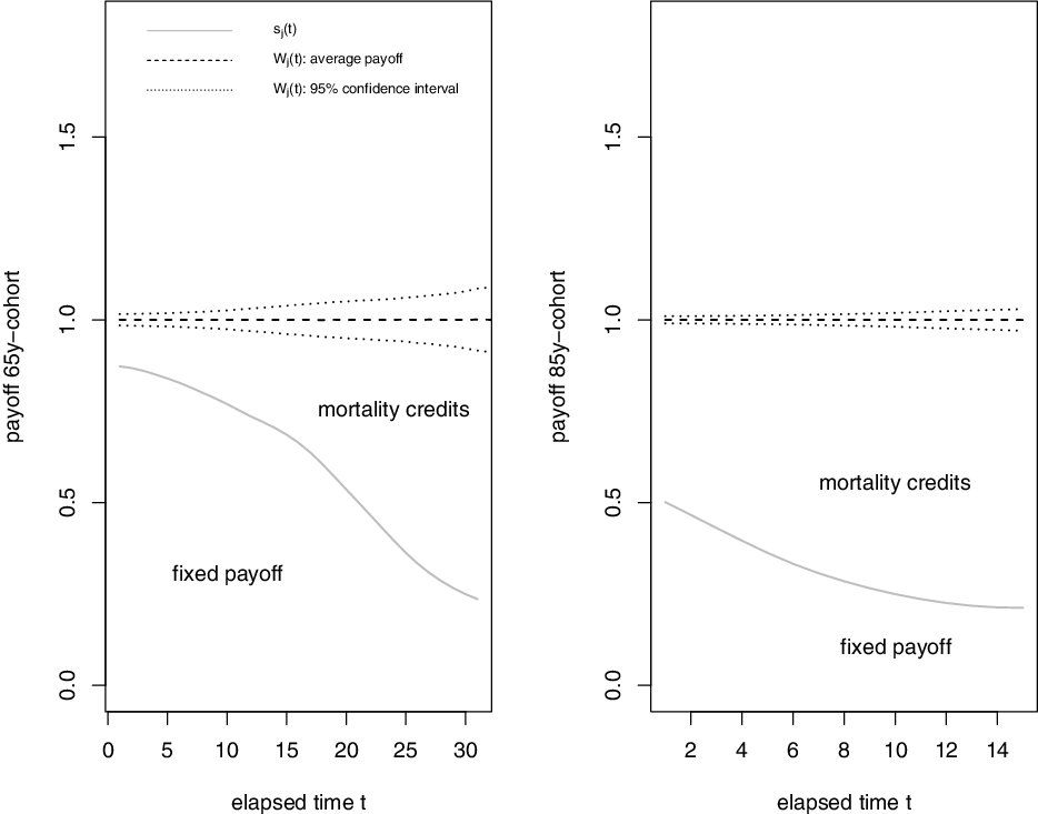
Figure 1. Evolution of fixed withdrawal
 $s_j(t)$
and total payoff
$s_j(t)$
and total payoff
 $W_j(t)$
(one simulation path), young (left) and old cohort (right). We use the conditional mean risk sharing rule for this illustrative example.
$W_j(t)$
(one simulation path), young (left) and old cohort (right). We use the conditional mean risk sharing rule for this illustrative example.
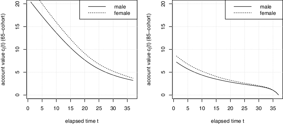
Figure 2. Evolution of the personal account
 $c_j(t)$
with time, young (left) and old cohort (right).
$c_j(t)$
with time, young (left) and old cohort (right).
2.C. Actuarial fairness
Equations (2.5) and (2.12), together with one of the sharing rules from Examples 2.2–2.4, fully define the payoff of a tontine in a 2-state framework. The first advantage of this scheme is that it allows to pool policyholders with different mortality risks, for example from different age cohorts. The second advantage is that it is actuarially fair in each period: at each time t, the expected discounted future payoffs to any individual j equal this individual’s current account value
 $c_j(t)$
, see Theorem 2.6.
$c_j(t)$
, see Theorem 2.6.
Theorem 2.6 (Actuarial fairness 2-state framework). The fairness condition (2.6) implies that the current account value (2.3) is actuarially fair at each time
 $t=0,1,\ldots, \omega-x_j$
, that is:
$t=0,1,\ldots, \omega-x_j$
, that is:
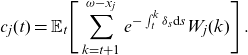 \begin{align}c_j(t) = \mathbb{E}_{t} \Bigg[\sum_{k=t+1}^{\omega-x_j} e^{- \int_{t}^k \delta_s \textrm{d}s} W_j(k)\Bigg]\,.\end{align}
The conditional mean risk-sharing rule (2.7), the linear sharing rule (2.8) and the linear regression rule (2.9) satisfy the fairness condition (2.6).
Proof. At time
 $t=\omega-x_j$
, individual j reaches the maximum possible age. The last year of life the individual only receives death benefits, and with (2.4) we get
$t=\omega-x_j$
, individual j reaches the maximum possible age. The last year of life the individual only receives death benefits, and with (2.4) we get
 $c_j(\omega-x_j) = 0$
. It implies that
$c_j(\omega-x_j) = 0$
. It implies that
 $c_j(\omega-x_j-1) = e^{- \int_{\omega-x_j-1}^{\omega-x_j} \delta_s \textrm{d}s} s_j(\omega-x_j) $
. We prove (2.13) by backwards induction. Assume that (2.13) holds for t. Using (2.3), (2.5) and (2.6), we find for an individual
$c_j(\omega-x_j-1) = e^{- \int_{\omega-x_j-1}^{\omega-x_j} \delta_s \textrm{d}s} s_j(\omega-x_j) $
. We prove (2.13) by backwards induction. Assume that (2.13) holds for t. Using (2.3), (2.5) and (2.6), we find for an individual
 $j\in\mathcal{L}_{t-1}$
:
$j\in\mathcal{L}_{t-1}$
:
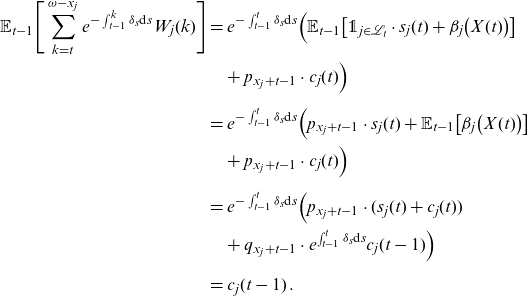 \begin{align*} \mathbb{E}_{t-1} \Bigg[\sum_{k=t}^{\omega-x_j} e^{- \int_{t-1}^k \delta_s \textrm{d}s} W_j(k)\Bigg] & = e^{- \int_{t-1}^t \delta_s \textrm{d}s} \Big(\mathbb{E}_{t-1} \big[\unicode[Times]{x1D7D9}_{j\in\mathcal{L}_t}\cdot s_j(t) + \beta_j\big(X(t) \big) \big] \\ & \quad + p_{x_j+t-1}\cdot c_j(t) \Big) \\[.2cm]& = e^{- \int_{t-1}^t \delta_s \textrm{d}s}\Big(p_{x_j+t-1}\cdot s_j(t) + \mathbb{E}_{t-1} \big[\beta_j\big(X(t) \big) \big] \\ & \quad + p_{x_j+t-1}\cdot c_j(t) \Big) \\[.2cm]& = e^{- \int_{t-1}^t \delta_s \textrm{d}s}\Big(p_{x_j+t-1}\cdot (s_j(t) + c_j(t)) \\ & \quad + q_{x_j+t-1}\cdot e^{\int_{t-1}^t \delta_s \textrm{d}s}c_j(t-1) \Big) \\[.2cm]&= c_j(t-1)\,.\end{align*}
This shows that (2.13) also holds for
 $t-1$
. Condition (2.6) is satisfied for the conditional mean risk-sharing rule as for each individual
$t-1$
. Condition (2.6) is satisfied for the conditional mean risk-sharing rule as for each individual
 $j \in \mathcal{L}_{t-1}$
:
$j \in \mathcal{L}_{t-1}$
:
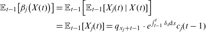 \begin{align*} \mathbb{E}_{t-1}\big[\beta_j\big(X(t) \big)\big] & =\mathbb{E}_{t-1}\Big[\mathbb{E}_{t-1}[X_j(t)\,|\,X(t)]\Big] \\ &= \mathbb{E}_{t-1}[X_j(t)] = q_{x_j+t-1} \cdot e^{\int_{t-1}^t \delta_s \textrm{d}s}c_j(t-1)\,\end{align*}
as well as for the linear risk-sharing rule as
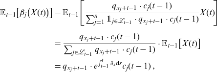 \begin{align*} \mathbb{E}_{t-1}\big[\beta_j\big(X(t) \big)\big] & = \mathbb{E}_{t-1}\Bigg[\frac{ q_{x_j+t-1}\cdot c_j(t-1) }{ \sum_{j=1}^n \unicode[Times]{x1D7D9}_{ j\in\mathcal{L}_{t-1}}\cdot q_{x_j+t-1}\cdot c_j(t-1) } X(t)\!\Bigg] \\[5pt]& = \frac{ q_{x_j+t-1}\cdot c_j(t-1) }{ \sum_{j \in \mathcal{L}_{t-1}} q_{x_j+t-1}\cdot c_j(t-1) } \cdot \mathbb{E}_{{t-1}}\big[X(t) \big] \\ & = q_{x_j+t-1}\cdot e^{\int_{t-1}^t \delta_s \textrm{d}s}c_j(t-1)\,,\end{align*}
and the linear regression rule:
 \begin{align*} \mathbb{E}_{t-1}\big[\! \beta_j\big(X(t) \big)\big] & = \mathbb{E}_{t-1}\Bigg[\mathbb{E}_{t-1}[X_j(t)] + \frac{\operatorname{Cov}_{t-1}[X_j(t),X(t)]}{\operatorname{Var}_{t-1}[X(t)]} \big(X(t)-\mathbb{E}_{t-1}[X(t)] \big)\!\Bigg] \\[5pt]& = \mathbb{E}_{t-1}[X_j(t)] =q_{x_j+t-1}\cdot e^{\int_{t-1}^t \delta_s \textrm{d}s}c_j(t-1)\,.\end{align*}
Theorem 2.6 demonstrates that our tontine scheme allows to share mortality risk between heterogeneous individuals (i.e. individuals with different life expectancies), see also Donnelly et al. (Reference Donnelly, Guillén and Nielsen2014), Milevsky and Salisbury (Reference Milevsky and Salisbury2015), Denuit (Reference Denuit2019). The fact that the scheme is fair at each time point t gives a second advantage: the design allows individuals to later join the tontine scheme at an actuarially fair price. By design, joining the scheme does not affect the average benefits of the existing members. In contrast, in a closed tontine scheme, the number of pool members is decreasing over time, leading to an increase in risk at old ages (see, e.g., Chen et al., Reference Chen, Hieber and Klein2019).
3. 3-state framework
In a second step, we extend the framework from the previous section to a life-care tontine and consider a 3-state semi-Markov model where any individual is either active (a), dependent (i) or dead (d). Initially, each individual is assumed to be in state active. In Section 3.1, we introduce additional notation for the 3-state model. We discuss the payoff of a life-care annuity in Section 3.2 before introducing our life-care tontine product together with the concept of morbidity credits in Section 3.3.
3.A. Additional notation
For an
 $x_j$
-year old individual, let us define:
$x_j$
-year old individual, let us define:
-
(a)
${}_tp_{x_j}^{aa}$
: the t-period sojourn probability in active state. -
(b)
$_{t}p_{x_j}^{ai}$
: the t-period transition probability from state a to i. Return from the dependent state to the active state is not possible. -
(c)
$_{1}p_{x_j}^{ad}=q_{x_j}^{(a)}$
and
$_{1}p_{x_j\;;\;z}^{id}=q_{x_j\;;\;z}^{(i)}$
: the annual death probabilities in state a and i, respectively. It is semi-Markovian in the latter case, with
$z=0,1,2 \ldots$
the time already spent in dependency.


The individual’s remaining lifetime
 $T_j$
is decomposed into:
$T_j$
is decomposed into:
 \begin{align}T_j=T_j^{(a)}+T_j^{(i)}\,,\end{align}
where
 $T_j^{(a)}$
is the time spent in autonomy and
$T_j^{(a)}$
is the time spent in autonomy and
 $T_j^{(i)}$
is the time spent in dependence or disability. We have
$T_j^{(i)}$
is the time spent in dependence or disability. We have
 $P(T_j^{(i)}=0)>0$
. Let us define the number of individuals in the active and dependent state, respectively, at a future time t:
$P(T_j^{(i)}=0)>0$
. Let us define the number of individuals in the active and dependent state, respectively, at a future time t:
 \begin{align} \mathcal{A}_t&\;:\!=\;\big\{\, j \in \mathcal{L}_t\,\big|\,T_j^{(a)}>t \big\}\,, \end{align}
 \begin{align} \mathcal{I}_{t\;;\;z} &\;:\!=\;\big\{\, j \in \mathcal{L}_t\,\big|\,T_j^{(a)}\leq t, T_j>t, z = t-T_j^{(a)} \big\} \,, \end{align}
 \begin{align} \mathcal{I}_t &\;:\!=\;\cup_{z=0}^{t-1} \mathcal{I}_{t\;;\;z} = \big\{\, j \in \mathcal{L}_t\,\big|\,T_j^{(a)}\leq t, T_j>t \big\} = \mathcal{L}_t \setminus \mathcal{A}_t\,.\end{align}
Relating this to the notation above, this means that
 ${}_tp_{x_j}^{aa} = \mathbb{E}[\unicode[Times]{x1D7D9}_{j \in \mathcal{A}_t}]$
,
${}_tp_{x_j}^{aa} = \mathbb{E}[\unicode[Times]{x1D7D9}_{j \in \mathcal{A}_t}]$
,
 ${}_tp_{x_j}^{ai} = \mathbb{E}[\unicode[Times]{x1D7D9}_{j \in \mathcal{I}_t}]$
,
${}_tp_{x_j}^{ai} = \mathbb{E}[\unicode[Times]{x1D7D9}_{j \in \mathcal{I}_t}]$
,
 $q_{x_j+t-1}^{(a)} = \mathbb{E}[\unicode[Times]{x1D7D9}_{j \in \mathcal{D}_t \cup \mathcal{A}_{t-1}}]$
,
$q_{x_j+t-1}^{(a)} = \mathbb{E}[\unicode[Times]{x1D7D9}_{j \in \mathcal{D}_t \cup \mathcal{A}_{t-1}}]$
,
 $q_{x_j+t-1\;;\;z}^{(i)} = \mathbb{E}[\unicode[Times]{x1D7D9}_{j \in \mathcal{D}_t \cup \mathcal{I}_{t-1\;;\;z-1} }] $
, and
$q_{x_j+t-1\;;\;z}^{(i)} = \mathbb{E}[\unicode[Times]{x1D7D9}_{j \in \mathcal{D}_t \cup \mathcal{I}_{t-1\;;\;z-1} }] $
, and
 $p_{x_j+t-1\;;\;z-1}^{ii} = \mathbb{E}[\unicode[Times]{x1D7D9}_{j \in \mathcal{L}_t \cup \mathcal{I}_{t-1\;;\;z-1}}]$
.
$p_{x_j+t-1\;;\;z-1}^{ii} = \mathbb{E}[\unicode[Times]{x1D7D9}_{j \in \mathcal{L}_t \cup \mathcal{I}_{t-1\;;\;z-1}}]$
.
3.B. Life-care annuity
In this section, we introduce life-care annuities and base ourselves on the works of, for example, Murtaugh et al. (Reference Murtaugh, Spillman, W and arshawsky2001), Spillman et al. (2003), Rickayzen (2007), Brown and Warshawsky (Reference Chen, Hieber and Klein2013), Shao et al. (2015) and Chen et al. (Reference Chen, Fuino, Sehner and Wagner2021). In contrast to the mutual insurance scheme discussed in this article, in a life-care annuity, mortality and morbidity risks are taken by an insurance provider. Each individual j pays the single premium
 $c_j(0)$
to buy an annuity with a future payment stream of
$c_j(0)$
to buy an annuity with a future payment stream of
 $b_j(t)$
,
$b_j(t)$
,
 $t=1,2,\ldots,\omega - x_j$
. This annuity is supplemented with an LTC cover that provides an annual amount of
$t=1,2,\ldots,\omega - x_j$
. This annuity is supplemented with an LTC cover that provides an annual amount of
 $(\alpha_j-1)\cdot b_j(t)$
as long as people are dependent.
$(\alpha_j-1)\cdot b_j(t)$
as long as people are dependent.
 $\alpha_j>1$
is an individual-specific constant reflecting an increased payoff in dependency. This additional LTC cover is an LTC annuity where the risk is taken by the insurance company. Ignoring administration and risk charges, the fair single premium
$\alpha_j>1$
is an individual-specific constant reflecting an increased payoff in dependency. This additional LTC cover is an LTC annuity where the risk is taken by the insurance company. Ignoring administration and risk charges, the fair single premium
 $c_j(0)$
of the life-care annuity is given by
$c_j(0)$
of the life-care annuity is given by
 \begin{align}c_j(0)=\sum_{t=1}^{\omega-x_j} \big({}_{t}p_{x_j}^{ai}\, e^{-\int_0^t \delta_s \textrm{d}s} \alpha_j \cdot b_j(t) + {}_{t}p_{x_j}^{aa}\, e^{-\int_0^t \delta_s \textrm{d}s} b_j(t) \big)\,.\end{align}
3.C. Life-care tontine
Based on the tontine scheme introduced in Section 2, we present a life-care tontine that on average provides the same payout as the life-care annuity from the previous Section 3.2. In a life-care tontine, payments are adapted according to the autonomy/dependence of an individual. We define by
 $c_j^{(a)}(t)$
and
$c_j^{(a)}(t)$
and
 $c_j^{(i)}(t\;;\;z)$
the current account values of an active and dependent individual, respectively; z indicates the time spent in dependency. Assuming that, at time 0, every individual is autonomous, we set
$c_j^{(i)}(t\;;\;z)$
the current account values of an active and dependent individual, respectively; z indicates the time spent in dependency. Assuming that, at time 0, every individual is autonomous, we set
 $c_j^{(a)}(0) = c_j(0)$
. The main idea is that individuals moving into the dependent state have a higher death probability than people staying in active state. If mortality credits in a tontine scheme account for this increase, the payments in dependency naturally increase. To define payments in a life-care tontine for an individual
$c_j^{(a)}(0) = c_j(0)$
. The main idea is that individuals moving into the dependent state have a higher death probability than people staying in active state. If mortality credits in a tontine scheme account for this increase, the payments in dependency naturally increase. To define payments in a life-care tontine for an individual
 $\;j\in\mathcal{L}_{t-1}$
, we modify the fairness condition (2.6) to distinguish between active (
$\;j\in\mathcal{L}_{t-1}$
, we modify the fairness condition (2.6) to distinguish between active (
 $\,j\in\mathcal{A}_{t-1}$
) and dependent individuals (
$\,j\in\mathcal{A}_{t-1}$
) and dependent individuals (
 $\,j\in\mathcal{I}_{t-1\;;\;z}$
), with z the time spent in dependency (in years):
$\,j\in\mathcal{I}_{t-1\;;\;z}$
), with z the time spent in dependency (in years):
 \begin{align} \mathbb{E}_{t-1}\big[\beta_j\big(X(t) \big)\,\big|\, j\in \mathcal{A}_{t-1} \big] =\, q^{(a)}_{x_j + t-1}\cdot e^{\int_{t-1}^t \delta_s \textrm{d}s}c_j^{(a)}(t-1) \,, \end{align}
 \begin{align} \mathbb{E}_{t-1}\big[\beta_j\big(X(t) \big)\,\big|\, j\in \mathcal{I}_{t-1\;;\;z} \big] =\, q^{(i)}_{x_j + t-1\;;\;z}\cdot e^{\int_{t-1}^t \delta_s \textrm{d}s}c_j^{(i)}(t-1\;;\;z) \,,\end{align}
where from now on,
 $\mathbb{E}_{t} \;:\!=\; \mathbb{E}[\,\cdot\,|\,\mathcal{F}_t]$
is an expectation conditional on the information
$\mathbb{E}_{t} \;:\!=\; \mathbb{E}[\,\cdot\,|\,\mathcal{F}_t]$
is an expectation conditional on the information
 $\mathcal{F}_t \;:\!=\; \sigma(\mathcal{A}_t, \mathcal{I}_{t;\;0},\mathcal{I}_{t;\;1},\ldots,\mathcal{I}_{t;\;t-1})$
. With this design, we apply Definition 2.1 to the 3-state framework. The increased death probability in dependency (
$\mathcal{F}_t \;:\!=\; \sigma(\mathcal{A}_t, \mathcal{I}_{t;\;0},\mathcal{I}_{t;\;1},\ldots,\mathcal{I}_{t;\;t-1})$
. With this design, we apply Definition 2.1 to the 3-state framework. The increased death probability in dependency (
 $q^{(i)}_{x_j + t-1\;;\;z}>q^{(a)}_{x_j + t-1}$
) increases the share of mortality credits and thus the overall payoff as soon as an individual moves from the active to the dependent state.
$q^{(i)}_{x_j + t-1\;;\;z}>q^{(a)}_{x_j + t-1}$
) increases the share of mortality credits and thus the overall payoff as soon as an individual moves from the active to the dependent state.
Again, the cash-flows satisfy the premium equivalence (2.1). In a tontine, the payoff to the pool (left hand side of (2.1)) is fixed, leaving the insurance provider with no mortality nor morbidity risk. The payoffs to the pool members
 $W_j(t)$
are random and depend on the mortality and morbidity in the pool.
$W_j(t)$
are random and depend on the mortality and morbidity in the pool.
3.C.1. Adjusting mortality credits to dependency
Mortality credits are now distributed according to the individual’s state (active, dependent, dead) using the fairness condition (3.6) and (3.7). We aim for an average payoff
 ${\alpha_j}\!\left(T^{(a)}\right)\cdot b_j(t)$
in dependency, where
${\alpha_j}\!\left(T^{(a)}\right)\cdot b_j(t)$
in dependency, where
 $\alpha_j(T^{(a)})$
is a constant that depends on the time spent in the active state. In our notation, this means that:
$\alpha_j(T^{(a)})$
is a constant that depends on the time spent in the active state. In our notation, this means that:
 \begin{align} \mathbb{E}[W_j(t) \,|\, j \in \mathcal{A}_t] = b_j(t)\,,\end{align}
 \begin{align} \mathbb{E}[W_j(t) \,|\, j \in \mathcal{I}_{t\;;\;t-T^{(a)}}] = \alpha_j\big(T^{(a)} \big) \cdot b_j(t)\, , \quad t\ge T^{(a)}.\end{align}
To achieve the desired average payoff (3.8) and (3.9) in the active and dependent state, respectively, we – as in Section 2 – decompose the payoff in a fixed and a variable part. The fixed part of individual j in the active and dependent state is denoted by
 $s_j^{(a)}(t)$
and
$s_j^{(a)}(t)$
and
 $s_j^{(i)}(t\;;\;z)$
, respectively. The pool observes time-t withdrawals
$s_j^{(i)}(t\;;\;z)$
, respectively. The pool observes time-t withdrawals
 $W_j(t)$
. For an individual
$W_j(t)$
. For an individual
 $j \in \mathcal{L}_{t-1}$
:
$j \in \mathcal{L}_{t-1}$
:
 \begin{align}W_j(t) & =\left\{ \begin{array}{ll} s_j^{(a)}(t) + \beta_j\big(X(t) \big)\,, & \mbox{if } j \in \mathcal{A}_{t} \\[.2cm] s_j^{(i)}(t\;;\;z) + \beta_j\big(X(t) \big) \,, & \mbox{if } j \in \mathcal{I}_{t\;;\;z} \\[.2cm] \beta_j\big(X(t)\big)\,\,, & \mbox{if } j \in \mathcal{D}_t. \\[.2cm] \end{array}\right.\end{align}
Starting with an initial account value of
 $c_j^{(a)}(0) = c_j(0)$
, the account for an active individual
$c_j^{(a)}(0) = c_j(0)$
, the account for an active individual
 $j\in\mathcal{A}_{t-1}$
(
$j\in\mathcal{A}_{t-1}$
(
 $t\le T^{(a)}, z \ge 1$
) evolves as in the 2-state framework, see (2.3):
$t\le T^{(a)}, z \ge 1$
) evolves as in the 2-state framework, see (2.3):
 \begin{align}c_j^{(a)}(t) = \left\{ \begin{array}{l@{\quad}l} e^{\int_{t-1}^t \delta_s \textrm{d}s} c_j^{(a)}(t-1) - s_j^{(a)}(t)\,, & j \in \mathcal{A}_{t}\;\;\;\quad and\quad t<T^{(a)} \\[.2cm] e^{\int_{t-1}^t \delta_s \textrm{d}s} c_j^{(a)}(t-1) - s_j^{(i)}(t\;;\;0)\,, & j \in \mathcal{I}_{t\;;\;0}\quad and\quad t=T^{(a)} \\[.2cm]0\,, & \textrm{otherwise}. \,\end{array}\right.\end{align}
The state-dependent constant
 $\alpha_j(T^{(a)})$
is chosen in a way that the product is actuarially fair, that is, at the time
$\alpha_j(T^{(a)})$
is chosen in a way that the product is actuarially fair, that is, at the time
 $T^{(a)}$
that an individual moves into dependency, the account value does not change:
$T^{(a)}$
that an individual moves into dependency, the account value does not change:
 \begin{align}\nonumber & \underbrace{c_j^{(i)}\big(T^{(a)};0\big)}_{\text{increased payoff for $t\ge T^{(a)}+1$}} + \underbrace{(\alpha_j(T^{(a)})-1) b_j(T^{(a)})}_{\text{increased payoff at time $T^{(a)}$}} \\[5pt]&\nonumber \qquad\quad = \mathbb{E}_{T^{(a)}} \Bigg[\sum_{k=T^{(a)}+1}^{\omega-x_j} e^{- \int_{T^{(a)}}^k \delta_s \textrm{d}s} W_j(k)\,\Bigg|\,j\in\mathcal{I}_{T^{(a)};0}\Bigg]+(\alpha_j(T^{(a)})-1) b_j(T^{(a)}) \\[5pt] &\quad\qquad = \mathbb{E}_{T^{(a)}} \Bigg[\sum_{k=T^{(a)}+1}^{\omega-x_j} e^{- \int_{T^{(a)}}^k \delta_s \textrm{d}s} W_j(k)\,\Bigg|\,j\in\mathcal{A}_{T^{(a)}}\Bigg] = c_j^{(a)}\big(T^{(a)}\big) \,.\end{align}
We choose the constants
 $\alpha_j(T^{(a)})$
such that (3.12) is satisfied. In dependency (
$\alpha_j(T^{(a)})$
such that (3.12) is satisfied. In dependency (
 $t>T^{(a)}$
,
$t>T^{(a)}$
,
 $j\in\mathcal{I}_{t-1}$
), the account value evolves as follows:
$j\in\mathcal{I}_{t-1}$
), the account value evolves as follows:
 \begin{align}c_j^{(i)}(t\;;\;z) = \left\{ \begin{array}{l@{\quad}l} e^{\int_{t-1}^t \delta_s \textrm{d}s} c_j^{(i)}(t-1\;;\;z-1) - s_j^{(i)}(t\;;\;z)\,, & j \in \mathcal{I}_{t} \\[5pt]0\,, & \textrm{otherwise}.\,\end{array}\right.\end{align}
The way to determine the payoff decomposition is presented in Theorem 3.1. Figure 3 gives a sample path for an active male person with an average payoff of
 $b_j(t)=1$
(left) and an individual that moves into dependency at time
$b_j(t)=1$
(left) and an individual that moves into dependency at time
 $T^{(a)}=15$
(right). The first years after moving into dependency are typically accompanied by a strong increase in mortality. In this case, the fixed part of the payoff even turns negative. Looking at the total payoff
$T^{(a)}=15$
(right). The first years after moving into dependency are typically accompanied by a strong increase in mortality. In this case, the fixed part of the payoff even turns negative. Looking at the total payoff
 $W_j(t)$
(dashed line) and its 95% confidence intervals (dotted line) in Figure 3, the slightly negative fixed payoff does not seem to be an issue: The total payoff is rather stable over time.
$W_j(t)$
(dashed line) and its 95% confidence intervals (dotted line) in Figure 3, the slightly negative fixed payoff does not seem to be an issue: The total payoff is rather stable over time.
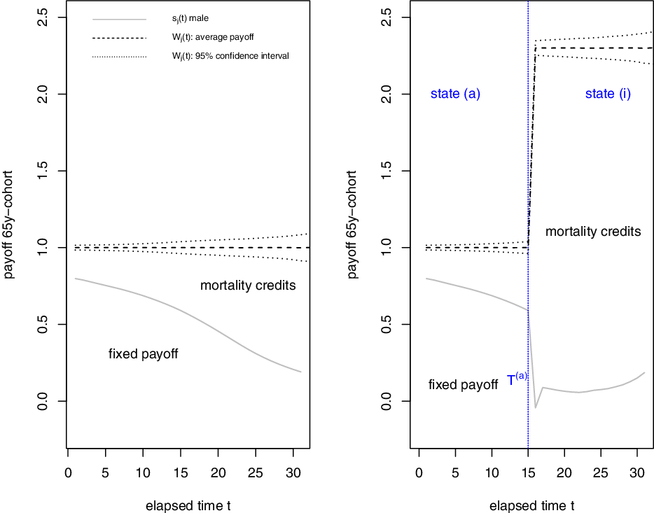
Figure 3. Evolution of fixed withdrawal
 $s_j^{(a)}(t)$
and
$s_j^{(a)}(t)$
and
 $s_j^{(i)}(t\;;\;t-T^{(a)})$
and total payoff
$s_j^{(i)}(t\;;\;t-T^{(a)})$
and total payoff
 $W_j(t)$
(one simulation path),
$W_j(t)$
(one simulation path),
 $x_j=65, T^{(a)}=\omega-x_j$
(left) and
$x_j=65, T^{(a)}=\omega-x_j$
(left) and
 $T^{(a)}=15$
(right).
$T^{(a)}=15$
(right).
Theorem 3.1 (Choice of
 $\alpha_j\big(T^{(a)} \big)$
,
$\alpha_j\big(T^{(a)} \big)$
,
 $s_j^{(a)}(t)$
,
$s_j^{(a)}(t)$
,
 $s_j^{(i)}(t\;;\;t-T^{(a)})$
) Consider an annual time grid
$s_j^{(i)}(t\;;\;t-T^{(a)})$
) Consider an annual time grid
 $t\in\mathbb{N}$
. An active individual (
$t\in\mathbb{N}$
. An active individual (
 $j\in\mathcal{A}_t$
) receives the fixed payoff
$j\in\mathcal{A}_t$
) receives the fixed payoff
 $s_j^{(a)}(t)$
determined via the backwards iteration:
$s_j^{(a)}(t)$
determined via the backwards iteration:
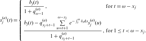 \begin{align} s_j^{(a)}(t) = \left\{ \begin{array}{ll} \dfrac{b_j(t)}{1+q^{(a)}_{\omega-1}}\,, & \text{for }t=\omega-x_j \\[12pt] \dfrac{ b_j(t) - q^{(a)}_{x_j+t-1} \sum\limits_{u=t+1}^{\omega-x_j} e^{-\int_t^u \delta_s\textrm{d}s} s_j^{(a)}(u)} {1+q^{(a)}_{x_j+t-1}}\,, & \text{for }1\le t < \omega-x_j. \end{array} \right.\end{align}
A dependent individual that spent
 $t-T^{(a)}$
years in dependency (
$t-T^{(a)}$
years in dependency (
 $j\in\mathcal{I}_{t\;;\; t-T^{(a)}}$
), receives for time
$j\in\mathcal{I}_{t\;;\; t-T^{(a)}}$
), receives for time
 $t\ge T^{(a)}$
the fixed payoff
$t\ge T^{(a)}$
the fixed payoff
 \begin{align}s_j^{(i)}\big(t\;;\;t-T^{(a)}\big)=\alpha_j(T^{(a)})\cdot \widetilde{s}_j^{\,(i)}(t\;;\;t-T^{(a)})\,,\end{align}
where
 $\widetilde{s}_j^{\,(i)}(t\;;\;t-T^{(a)})$
is, for
$\widetilde{s}_j^{\,(i)}(t\;;\;t-T^{(a)})$
is, for
 $t\ge T^{(a)}$
, determined via the backwards iteration:
$t\ge T^{(a)}$
, determined via the backwards iteration:
 \begin{align} & \widetilde{s}_j^{\,(i)}(t\;;\;t-T^{(a)}) = \nonumber \\[5pt] & \left\{ \begin{array}{ll} \dfrac{b_j(t)}{1+q^{(i)}_{\omega-1;t-T^{(a)}-1}}\,, & \text{for }t=\omega-x_j \\[.2cm] \dfrac{ b_j(t) - q^{(i)}_{x_j+t-1;t-T^{(a)}-1} \sum\limits_{u=t+1}^{\omega-x_j} e^{-\int_t^u \delta_s\textrm{d}s} \,\widetilde{s}_j^{\,(i)}(u;u-T^{(a)})} {1+q^{(i)}_{x_j+t-1;t-T^{(a)}-1}}\,, & \text{for }T^{(a)} \leq t < \omega-x_j. \end{array} \right.\end{align}
The factor
 $\alpha_j(T^{(a)})$
that increases payments in dependency is determined via:
$\alpha_j(T^{(a)})$
that increases payments in dependency is determined via:
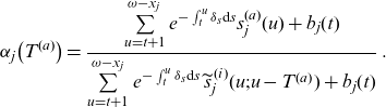 \begin{align}& \alpha_j\big(T^{(a)}\big)=\frac{\sum\limits_{u=t+1}^{\omega-x_j} e^{-\int_t^u \delta_s\textrm{d}s } {s}_j^{(a)}(u)+b_j(t)}{\sum\limits_{u=t+1}^{\omega-x_j} e^{-\int_t^u \delta_s\textrm{d}s } \, \widetilde{s}_j^{\,(i)}(u;u-T^{(a)})+b_j(t)}\,.\end{align}
Proof. See Appendix A.
Figure 4 presents the function
 $\alpha_j (T^{(a)})$
in our data set, the table DAV2008P provided by the German Actuarial Society, see also the online appendix for a detailed description. If
$\alpha_j (T^{(a)})$
in our data set, the table DAV2008P provided by the German Actuarial Society, see also the online appendix for a detailed description. If
 $\alpha_j (T^{(a)})=1$
, this would mean that an individual in dependency would receive, on average, the same payoff as if he/she were active. We want to stress that the higher payoff in dependency does not necessarily lead to an increase in present value of the individual: this remains a tradeoff between the increase in mortality rates and the increase in payoff. From our data, we observe that a fair value of
$\alpha_j (T^{(a)})=1$
, this would mean that an individual in dependency would receive, on average, the same payoff as if he/she were active. We want to stress that the higher payoff in dependency does not necessarily lead to an increase in present value of the individual: this remains a tradeoff between the increase in mortality rates and the increase in payoff. From our data, we observe that a fair value of
 $\alpha_j (T^{(a)})$
takes values between 2 and 4 which implies a considerable increase of benefits in dependency, that is a dependent individual may receive a 2-4 times higher payoff than an active individual. The increase strongly depends on the time
$\alpha_j (T^{(a)})$
takes values between 2 and 4 which implies a considerable increase of benefits in dependency, that is a dependent individual may receive a 2-4 times higher payoff than an active individual. The increase strongly depends on the time
 $T^{(a)}$
the person moves into dependency. If we want to fix the increase in dependency, say to
$T^{(a)}$
the person moves into dependency. If we want to fix the increase in dependency, say to
 $\alpha_j(T^{(a)}) = \alpha_j$
as in the case of the life-care annuity in Section 3.B, we need to share the corresponding loss/gain that appears if somebody moves into dependency, see the following section.
$\alpha_j(T^{(a)}) = \alpha_j$
as in the case of the life-care annuity in Section 3.B, we need to share the corresponding loss/gain that appears if somebody moves into dependency, see the following section.
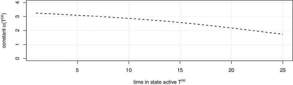
Figure 4. Adjustment constant
 $\alpha_j(T^{(a)})$
for an
$\alpha_j(T^{(a)})$
for an
 $x_j=65$
year old as a function of the time in the active state
$x_j=65$
year old as a function of the time in the active state
 $T^{(a)}$
(if
$T^{(a)}$
(if
 $T^{(i)}>0$
).
$T^{(i)}>0$
).
3.C.2. A priori fixation of
$\alpha_j(T^{(a)})$

As a next step, we want to fix the payoff in dependency with a predetermined increase in the dependent state to
 $\alpha_j$
. In other words, we want to smooth
$\alpha_j$
. In other words, we want to smooth
 $\alpha_j\big(T^{(a)} \big)$
from the previous section (see Figure 4). A gain/deficit from this payoff adjustment is shared within the pool by so-called morbidity credits. Formally, denote as
$\alpha_j\big(T^{(a)} \big)$
from the previous section (see Figure 4). A gain/deficit from this payoff adjustment is shared within the pool by so-called morbidity credits. Formally, denote as
 \begin{align*}Y_j(t) \;:\!=\; \unicode[Times]{x1D7D9}_{ j\in \mathcal{I}_{t\;;\;0} } \Big(\big(c_j^{(a)}(t) - c_j^{(i)}(t\;;\;0) \big)+ \big(1-\alpha_j\big) b_j(t) \Big)\end{align*}
the morbidity credits for individual j. Morbidity credits are needed to adjust the benefits of individuals that have moved to the dependent state in
 $(t-1,t]$
and are still alive at time t (that is an individual
$(t-1,t]$
and are still alive at time t (that is an individual
 $j\in \mathcal{I}_{t\;;\;0}$
). They contain two parts:
$j\in \mathcal{I}_{t\;;\;0}$
). They contain two parts:
 $\big(1-\alpha_j\big) b_j(t)$
increases the payoff at the first payoff date after moving into dependency while
$\big(1-\alpha_j\big) b_j(t)$
increases the payoff at the first payoff date after moving into dependency while
 $\big(c_j^{(a)}(t) - c_j^{(i)}(t\;;\;0) \big)$
adjusts the later payoffs. The morbidity credits are redistributed among the pool of individuals. Note that they can be positive or negative, depending on whether the
$\big(c_j^{(a)}(t) - c_j^{(i)}(t\;;\;0) \big)$
adjusts the later payoffs. The morbidity credits are redistributed among the pool of individuals. Note that they can be positive or negative, depending on whether the
 $\alpha_j\big(T^{(a)} \big)$
-value is higher or lower than the “fair” increase determined in the previous section (for our data set, see the values presented in Figure 4). At each time
$\alpha_j\big(T^{(a)} \big)$
-value is higher or lower than the “fair” increase determined in the previous section (for our data set, see the values presented in Figure 4). At each time
 $t=1,2,\ldots,T$
, we have to distribute
$t=1,2,\ldots,T$
, we have to distribute
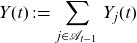 \begin{align*}Y(t) \;:\!=\; \sum_{j \in \mathcal{A}_{t-1} } Y_j(t)\end{align*}
according to some predefined rule. We, similarly to the concept of mortality credits in the previous section, introduce a function
 $\gamma_j\big(Y(t) \big)$
that redistributes the morbidity credits Y(t) within the pool, see Definition 3.2.
$\gamma_j\big(Y(t) \big)$
that redistributes the morbidity credits Y(t) within the pool, see Definition 3.2.
Definition 3.2 (Fair distribution rule: morbidity credits) If the share distributed to individual
 $j\in\mathcal{L}_{t-1}$
is denoted by
$j\in\mathcal{L}_{t-1}$
is denoted by
 $ \gamma_j\big(Y(t) \big)$
, a fair distribution rule has to satisfy the following properties:
$ \gamma_j\big(Y(t) \big)$
, a fair distribution rule has to satisfy the following properties:
-
• Self-sufficiency property:
$\sum_{j\in\mathcal{L}_{t-1}} \gamma_j\big(Y(t) \big) = Y(t)$
. -
• Fairness property:
(3.18)
\begin{align} & \mathbb{E}_{t-1}\big[\gamma_j\big(Y(t) \big)\,\big] \quad= \underbrace{\mathbb{E}_{t-1}\big[\unicode[Times]{x1D7D9}_{j \in \mathcal{I}_{t\;;\;0}} \big]}_{\text{probability to get dependent in $(t-1,t]$}} \nonumber \\[5pt] & \qquad \qquad\qquad\qquad \qquad \qquad \qquad\qquad \cdot \underbrace{\big(c_j^{(a)}(t)-c_j^{(i)}(t)+\big(1-\alpha_j\big) b_j(t)\big) }_{\text{required capital at time t}} \,.\end{align}


Again, we can, for example, choose a conditional mean risk-sharing, linear sharing or linear regression rule as a distribution rule
 $\gamma_j(\!\cdot\!)$
. For an active individual, we can rewrite (3.18) to obtain
$\gamma_j(\!\cdot\!)$
. For an active individual, we can rewrite (3.18) to obtain
 \begin{align} & \mathbb{E}_{t-1}\big[\gamma_j\big(Y(t) \big)\,\big|\,j\in\mathcal{A}_{t-1} \big] = p_{x_j + t-1}^{ai} \cdot \big(c_j^{(a)}(t)-c_j^{(i)}(t)+s_j^{(a)}(t)-s_j^{(i)}(t)\big)\,.\end{align}
If the individual is dependent or dead already at time
 $t-1$
, we obtain
$t-1$
, we obtain
 $\mathbb{E}_{t-1}[\gamma_j(Y(t))\,|\, j\in \mathcal{I}_{t-1}] =\mathbb{E}_{t-1}[\gamma_j(Y(t))\,|\, j\in \mathcal{D}_{t-1}] = 0 $
, that is in a fair distribution scheme dead or dependent people do (on average) not receive any morbidity credits. In our tontine scheme, we thus redistribute the credits among active individuals
$\mathbb{E}_{t-1}[\gamma_j(Y(t))\,|\, j\in \mathcal{I}_{t-1}] =\mathbb{E}_{t-1}[\gamma_j(Y(t))\,|\, j\in \mathcal{D}_{t-1}] = 0 $
, that is in a fair distribution scheme dead or dependent people do (on average) not receive any morbidity credits. In our tontine scheme, we thus redistribute the credits among active individuals
 $j\in \mathcal{A}_{t-1}$
only. In a later extension, it might make sense to share the risk
$j\in \mathcal{A}_{t-1}$
only. In a later extension, it might make sense to share the risk
 $Y(t)-\mathbb{E}_{t-1}[Y(t)]$
among all survivors
$Y(t)-\mathbb{E}_{t-1}[Y(t)]$
among all survivors
 $j\in\mathcal{L}_{t-1}$
. The pool observes time-t withdrawals
$j\in\mathcal{L}_{t-1}$
. The pool observes time-t withdrawals
 $W_j(t)$
, decomposed into a fixed withdrawal, mortality and morbidity credits. For an active individual
$W_j(t)$
, decomposed into a fixed withdrawal, mortality and morbidity credits. For an active individual
 $j \in \mathcal{A}_{t-1}$
:
$j \in \mathcal{A}_{t-1}$
:
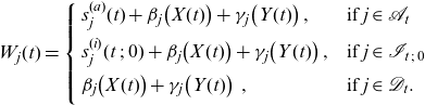 \begin{align}W_j(t) & =\left\{ \begin{array}{l@{\quad}l} s_j^{(a)}(t) + \beta_j\big(X(t) \big) + \gamma_j\big(Y(t) \big)\,, & \mbox{if } j \in \mathcal{A}_{t} \\[.2cm] s_j^{(i)}(t\;;\;0) + \beta_j\big(X(t) \big) + \gamma_j\big(Y(t) \big)\,, & \mbox{if } j \in \mathcal{I}_{t\;;\;0} \\[.2cm] \beta_j\big(X(t)\big)+\gamma_j\big(Y(t) \big)\,\,, & \mbox{if } j \in \mathcal{D}_t. \\[.2cm] \end{array}\right.\end{align}
For a dependent individual
 $j \in \mathcal{I}_{t-1}$
that moved into dependency at time
$j \in \mathcal{I}_{t-1}$
that moved into dependency at time
 $T^{(a)}<t$
:
$T^{(a)}<t$
:
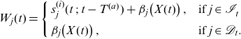 \begin{align}W_j(t) & =\left\{ \begin{array}{l@{\quad}l} s_j^{(i)}(t\;;\;t-T^{(a)}) + \beta_j\big(X(t) \big) \,, & \mbox{if } j \in \mathcal{I}_{t}^{^{^{\,}}} \, \\[.2cm] \beta_j\big(X(t)\big)\,, & \mbox{if } j \in \mathcal{D}_t. \end{array}\right.\end{align}
Figure 5 illustrates one simulation run in the 3-state framework, comparing an active person (left) to an individual moving into dependency at time
 $T^{(a)}=15$
. The product is shown to be actuarially fair in Theorem 3.3.
$T^{(a)}=15$
. The product is shown to be actuarially fair in Theorem 3.3.
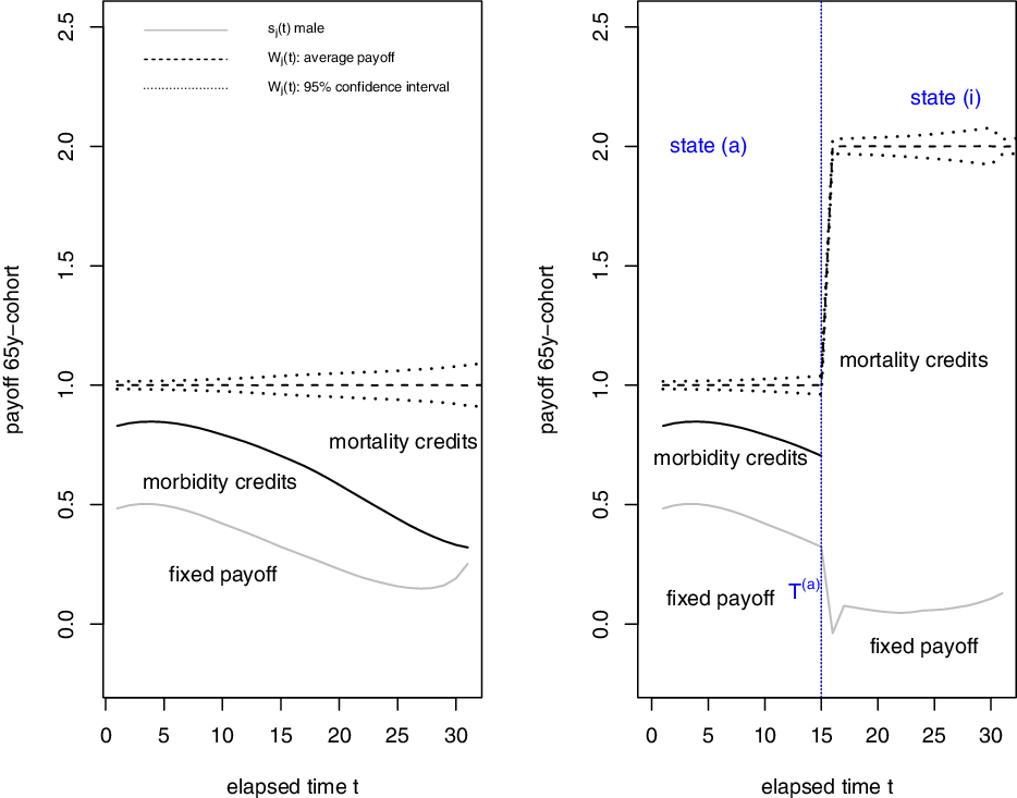
Figure 5. Evolution of fixed withdrawal
 $s_j^{(a)}(t)$
and
$s_j^{(a)}(t)$
and
 $s_j^{(i)}(t\;;\;t-T^{(a)})$
and total payoff
$s_j^{(i)}(t\;;\;t-T^{(a)})$
and total payoff
 $W_j(t)$
(one simulation path),
$W_j(t)$
(one simulation path),
 $x_j=65, T^{(a)}=\omega-x_j$
(left) and
$x_j=65, T^{(a)}=\omega-x_j$
(left) and
 $T^{(a)}=15$
(right).
$T^{(a)}=15$
(right).
Theorem 3.3 (Actuarial fairness 3-state framework). The fairness conditions (3.6), (3.7) and (3.18) imply that the current account value is actuarially fair for a dependent individual if, at each time
 $t=T^{(a)},\ldots, \omega-x_j$
:
$t=T^{(a)},\ldots, \omega-x_j$
:
 \begin{align}c_j^{(i)}\big(t\;;\;t-T^{(a)}\big) = \mathbb{E}_{t} \Bigg[\sum_{k=t+1}^{\omega-x_j} e^{- \int_{t}^k \delta_s \textrm{d}s} W_j(k) \, \Bigg|\, j \in \mathcal{I}_{t\;;\;t-T^{(a)}}\Bigg]\,.\end{align}
Similarly, it is actuarially fair for an active individual as, at each time
 $t=0,1,\ldots, \omega-x_j$
:
$t=0,1,\ldots, \omega-x_j$
:
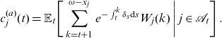 \begin{align}c_j^{(a)}(t) = \mathbb{E}_{t} \Bigg[\sum_{k=t+1}^{\omega-x_j} e^{- \int_{t}^k \delta_s \textrm{d}s} W_j(k) \,\Bigg|\, j \in \mathcal{A}_{t}\Bigg]\, .\end{align}
Proof. See Appendix B.
Note that at time
 $t=T^{(a)}$
, we have that
$t=T^{(a)}$
, we have that
 $s_j^{(a)}(t) - s_j^{(i)}(t\;;\;0)=(1-\alpha_{j})b_j(t)$
. As in the 2-state framework, the payoff is split into a fixed part, mortality and morbidity credits in a way that we obtain a desired average payoff. For an active individual, this average payoff is
$s_j^{(a)}(t) - s_j^{(i)}(t\;;\;0)=(1-\alpha_{j})b_j(t)$
. As in the 2-state framework, the payoff is split into a fixed part, mortality and morbidity credits in a way that we obtain a desired average payoff. For an active individual, this average payoff is
 $b_j(t)$
, while for a dependent individual it is increased to
$b_j(t)$
, while for a dependent individual it is increased to
 $\alpha_j \cdot b_j(t)$
, where
$\alpha_j \cdot b_j(t)$
, where
 $\alpha_j>1$
is a predetermined constant. In the 3-state framework, we need to separately look at active and dependent individuals, as they have different time patterns of average mortality and morbidity credits. Mortality credits are shared within the whole group. However, dependent individuals receive a larger share of these credits due to their higher mortality risk. Theorem 3.4 shows how to determine the fixed part of the payoff and the account values for active and dependent individuals, respectively.
$\alpha_j>1$
is a predetermined constant. In the 3-state framework, we need to separately look at active and dependent individuals, as they have different time patterns of average mortality and morbidity credits. Mortality credits are shared within the whole group. However, dependent individuals receive a larger share of these credits due to their higher mortality risk. Theorem 3.4 shows how to determine the fixed part of the payoff and the account values for active and dependent individuals, respectively.
Theorem 3.4 (Choice of
 $s_j^{(a)}(t)$
,
$s_j^{(a)}(t)$
,
 $s_j^{(i)}(t\;;\;t-T^{(a)})$
) Consider an annual time grid
$s_j^{(i)}(t\;;\;t-T^{(a)})$
) Consider an annual time grid
 $t\in\mathbb{N}$
. For a dependent individual (
$t\in\mathbb{N}$
. For a dependent individual (
 $j\in\mathcal{I}_t$
), we follow Theorem 3.1 and use (3.16) to obtain for each
$j\in\mathcal{I}_t$
), we follow Theorem 3.1 and use (3.16) to obtain for each
 $T^{(a)}=1,2,\ldots,\omega-x_j-1$
:
$T^{(a)}=1,2,\ldots,\omega-x_j-1$
:
 \begin{align}s_j^{(i)}\big(t\;;\;t-T^{(a)}\big)=\alpha_j\cdot \widetilde{s}_j^{\,(i)}(t\;;\;t-T^{(a)}),\text{ for }t=T^{(a)}+1,T^{(a)}+2,\ldots\end{align}
and the corresponding account value at time
 $t\ge T^{(a)}$
:
$t\ge T^{(a)}$
:
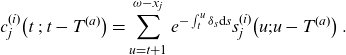 \begin{align}c_j^{(i)}\big(t\;;\;t-T^{(a)}\big)=\sum_{u=t+1}^{\omega-x_j} e^{-\int_{t}^u \delta_s \textrm{d}s} s^{(i)}_j\big(u;u-T^{(a)}\big)\,.\end{align}
An active individual (
 $j\in\mathcal{A}_t$
) receives the fixed payoff
$j\in\mathcal{A}_t$
) receives the fixed payoff
 $s_j^{(a)}(t)$
determined via the backwards iteration:
$s_j^{(a)}(t)$
determined via the backwards iteration:
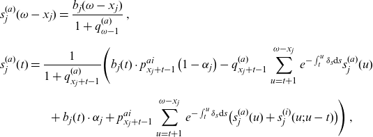 \begin{align}& s_j^{(a)}(\omega-x_j) = \frac{b_j(\omega-x_j)}{1+q_{\omega-1}^{(a)}}\,, \nonumber \\[5pt] \nonumber & s_j^{(a)}(t) = \frac{1}{1+q_{x_j+t-1}^{(a)}} \Bigg(b_j(t) \cdot p^{ai}_{x_j+t-1} \big(1-\alpha_j \big) - q_{x_j+t-1}^{(a)} \sum\limits_{u=t+1}^{\omega-x_j} e^{-\int_{t}^u \delta_s \textrm{d}s} s_j^{(a)}(u) \\[5pt]& \qquad\qquad + b_j(t) \cdot \alpha_j + p_{x_j+t-1}^{ai} \sum\limits_{u=t+1}^{\omega-x_j} e^{-\int_{t}^u \delta_s \textrm{d}s} \big(s_j^{(a)}(u)+s_j^{(i)}(u;u-t)\big) \Bigg) \,, \end{align}
 \begin{align}\nonumber & \quad \text{for }t=\omega-x_j-1,\omega-x_j-2,\ldots,1\,.\end{align}
At time
 $T^{(a)}$
, we have that:
$T^{(a)}$
, we have that:
 \begin{align}s^{(i)}_j(T^{(a)};0)=s^{(a)}_j(T^{(a)})+(\alpha_j-1) b_j(T^{(a)})\,.\end{align}
Proof. See Appendix C.
As in the 2-state case, the computation of the fixed components of the payoff
 $s_j^{(a)}(t)$
,
$s_j^{(a)}(t)$
,
 $s_j^{(i)}(t\;;\;t-T^{(a)})$
can be carried out for each individual separately.
$s_j^{(i)}(t\;;\;t-T^{(a)})$
can be carried out for each individual separately.
4. Outlook, further research and practical implications
The paper relies on the sharing of mortality and morbidity risk. Several simplifying assumptions were used, and they might be relaxed in future research. This short section highlights several interesting research questions, some practical implications, and possible extensions.
First, in the numerical examples, we assume that each individual’s mortality and morbidity risk is independent of the other pool members’ risk. This is only true if there are no systematic risks affecting every pool member simultaneously, like a pandemic, improved medication or a general increase in life expectancy. The existence of systematic morbidity risk is still controversially discussed (for example, Fries, Reference Fries1980 detects a rectangulariation of morbidity, while Fuino and Wagner, Reference Fuino and Wagner2020 find that “the duration of LTC has not significantly changed in the period from 1995 to 2009”). It would be interesting to analyze the life-care tontine in a fully calibrated mortality and morbidity risk model that accounts for systematic risk factors (see, for example, the model frameworks of Christiansen et al., Reference Christiansen, Denuit and Dhaene2014; Li et al., Reference Li, Shao and Sherris2017; Sherris and Wei, Reference Sherris and Wei2021). For systematic mortality risk models applied to tontines and pooled annuities, see, for example, Qiao and Sherris (Reference Qiao and Sherris2013), Chen et al. (Reference Chen, Fuino, Sehner and Wagner2021). Our assumption of independent remaining lifetimes can easily be relaxed as the separation in fixed payoff, mortality and morbidity risk can be carried out separately for each individual. In this derivation, there is no constraint on the dependence structure between individual lifetimes.
In our framework, each individual receives the same investment return (see also Donnelly et al., Reference Donnelly, Guillén and Nielsen2014 for a stochastic version of this setting). In participating life insurance, however, this is not always the case as contracts with different guaranteed rates are pooled (see, for example, Hansen and Miltersen, Reference Hansen and Miltersen2002; Hieber et al., Reference Hieber, Natolski and Werner2019). It might be interesting to discuss an actuarially fair risk sharing scheme where both mortality and financial risk are heterogeneous between individual contracts.
Last, it might be worthwhile to explore more complex mutual insurance schemes. Instead of purely investing in a mutual insurance scheme, it might make sense to combine traditional retirement products and mutual insurance (see, e.g., Chen et al., Reference Chen, Hieber and Klein2019; Chen et al., Reference Chen, Rach and Sehner2020; Weinert and Gründl, Reference Weinert and Gründl2021). For such schemes, the analysis of the interplay between heterogeneity and income stability is an interesting path for future research (see also, for example, Bernhardt and Qu, Reference Bernhardt and Qu2022; Denuit et al., Reference Denuit, Hieber and Robert2022).
5. Conclusion
We designed a novel mutual insurance scheme called life-care tontine and discuss its potential use in an LTC cover perspective. The product relies on the natural hedge inherent between mortality and morbidity risks. When moving into dependency, individuals may need a higher payoff for a shorter remaining lifetime, allowing to easily pool these risks with healthy individuals. As in the case of a life-care annuity, the pooling of mortality and morbidity risks reduces adverse selection costs and provides more people access to LTC insurance. Further, the insurance provider is merely administrative, leading to a significant reduction in risk and administration charges (see, e.g., Chen et al., Reference Chen, Hieber and Klein2019). The drawback naturally is that the systematic risk lies with the policyholders. A major innovation is the development of a creative product design: cashflows can be smoothed to fit the current and future needs of the market. The product is actuarially fair at each point in time, allowing people to later join the tontine scheme. The individual flexibility of our payoff design answers the individual practical needs of the insureds. Technically, we rely on a backward iteration used to deduce the smoothed cashflows patterns and the separation of cash-flows in a fixed withdrawal, mortality and morbidity credits. The flexibility and fairness of the system results from the fact that this iteration can be carried out individually for each pool member. The pooling scheme shares the mortality and morbidity risks within the pool. An increase in pool size reduces the volatility of the payoff but not the average payoff to each individual. The average future payoffs are based on each individual’s risk, for example, the age and health status. The 2-state and 3-state models are applied to real life data, providing coherent simulations and illustrating the adequacy of our product framework.
Acknowledgements
We gratefully acknowledge the extremely valuable scientific discussions with Michel Denuit (UC Louvain). We also thank participants of the 5th Ulm Actuarial Days 2020, the 24th (Virtual) International Congress on Insurance: Mathematics and Economics (IME) 2021 and the ASTIN-AFIR colloquium 2021 for many useful comments. We also appreciate suggestions by An Chen, Marcus Christiansen and two anonymous referees. The paper was awarded the AFIR-ERM best paper award 2021.
Funding
Peter Hieber was supported by the PRIME programme of the German Academic Exchange Service (DAAD) with funds from the German Federal Ministry of Education and Research (BMBF).
Supplementary material
To view supplementary material for this article, please visit http://dx.doi.org/10.1017/asb.2022.6.
Appendix A. Proof of Theorem 3.1
The payoff
 $\widetilde{s}_j^{\,(i)}(t\;;\;t-T^{(a)})$
for a dependent individual
$\widetilde{s}_j^{\,(i)}(t\;;\;t-T^{(a)})$
for a dependent individual
 $j\in\mathcal{I}_t$
receiving an average payoff
$j\in\mathcal{I}_t$
receiving an average payoff
 $b_j(t)$
at times
$b_j(t)$
at times
 $t\ge T^{(a)}$
is obtained using the 2-state semi-Markov backwards iteration system (3.14), see also the similar iteration in Section 2, Equation (2.12).
$t\ge T^{(a)}$
is obtained using the 2-state semi-Markov backwards iteration system (3.14), see also the similar iteration in Section 2, Equation (2.12).
As we do not allow for additional payments in dependency, we want to choose
 $\alpha_j(T^{(a)})$
in (3.15) such that the present value of future payoffs does not change if a person moves to dependency, that is (3.12) is satisfied. This implies, for an active individual
$\alpha_j(T^{(a)})$
in (3.15) such that the present value of future payoffs does not change if a person moves to dependency, that is (3.12) is satisfied. This implies, for an active individual
 $j \in A_{t-1}$
:
$j \in A_{t-1}$
:
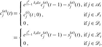 \begin{align*}c_j^{(a)}(t)&=\left\{ \begin{array}{ll} e^{\int_{t-1}^{t} \delta_{s} \textrm{d}s} c_{j}^{(a)}(t-1)-s_j^{(a)}(t) \,, & \mbox{if } j \in \mathcal{A}_t \\[.2cm] c_j^{(i)}(t\;;\;0) \,, & \mbox{if } j \in \mathcal{I}_t \\[.2cm] 0 \,, & \mbox{if } j \in \mathcal{D}_t \end{array}\right. \\ &=\left\{ \begin{array}{ll} e^{\int_{t-1}^{t} \delta_{s} \textrm{d}s} c_{j}^{(a)}(t-1) - s_j^{(a)}(t) \,, & \mbox{if } j \in \mathcal{L}_t^{^{^{^{^{^{\,}}}}}} \\[.2cm] 0 \,, & \mbox{if } j \in \mathcal{D}_t. \end{array}\right.\end{align*}
As in Section 2, Equation (2.12), we can solve this system to obtain:
 \begin{align}c_j^{(a)}(t)= \sum_{u=t+1}^{T}e^{\int_{t}^{u} \delta_{s} \textrm{d}s} \, s_j^{(a)}(u)\,.\end{align}
The backward iteration (3.14) determines the fixed part of the payoff
 $s_j^{(a)}(t)$
for an active individual, see also the 2-state framework in Section 2, Equation (2.12).
$s_j^{(a)}(t)$
for an active individual, see also the 2-state framework in Section 2, Equation (2.12).
Let us name
 $\widetilde{c}_j^{\,(i)}(t\;;\;t-T^{(a)})$
the reference amount, based on a predetermined
$\widetilde{c}_j^{\,(i)}(t\;;\;t-T^{(a)})$
the reference amount, based on a predetermined
 $\alpha_j(T^{(a)})$
-value of 1 and the corresponding fixed payments
$\alpha_j(T^{(a)})$
-value of 1 and the corresponding fixed payments
 $\widetilde{s}_j^{\,(i)}(t\;;\;t-T^{(a)})$
. We have
$\widetilde{s}_j^{\,(i)}(t\;;\;t-T^{(a)})$
. We have
 \[s_j^{(i)}\big(t\;;\;t-T^{(a)}\big)=\alpha_j\big(T^{(a)} \big)\cdot \widetilde{s}_j^{\,(i)}(t\;;\;t-T^{(a)})\,. \]
It is deduced that
 \[c_j^{(i)}\big(t\;;\;t-T^{(a)}\big)=\alpha_j\big(T^{(a)}\big)\cdot \widetilde{c}_j^{\,(i)}(t\;;\;t-T^{(a)})\,.\]
We solve for
 $\alpha$
in (3.12). If we use (3.12), that is if we assume that the present value of future payoffs is unchanged if a person moves into dependency, we obtain
$\alpha$
in (3.12). If we use (3.12), that is if we assume that the present value of future payoffs is unchanged if a person moves into dependency, we obtain
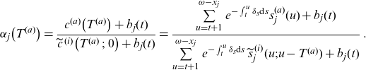 \begin{align*}& \alpha_j\big(T^{(a)}\big)=\frac{c^{(a)}\big(T^{(a)}\big)+b_j(t)} {\widetilde{c}^{\,(i)}\big(T^{(a)}\;;\;0\big)+b_j(t)} =\frac{\sum\limits_{u=t+1}^{\omega-x_j} e^{-\int_t^u \delta_s\textrm{d}s } {s}_j^{(a)}(u)+b_j(t)}{\sum\limits_{u=t+1}^{\omega-x_j} e^{-\int_t^u \delta_s\textrm{d}s } \, \widetilde{s}_j^{\,(i)}(u;u-T^{(a)})+b_j(t)}\,.\end{align*}
Appendix B. Proof of Theorem 3.3
At time
 $\omega-x_j$
, we have
$\omega-x_j$
, we have
 $q^{(i)}_{\omega\;;\;z}=1$
and the cash flows only consist of mortality credits. Fairness condition (3.7) is supposed to hold implying
$q^{(i)}_{\omega\;;\;z}=1$
and the cash flows only consist of mortality credits. Fairness condition (3.7) is supposed to hold implying
 $c_j^{(i)}(\omega-x_j\;;\;z)=0, \forall z$
. Assume that (3.22) holds for time t. For a dependent person
$c_j^{(i)}(\omega-x_j\;;\;z)=0, \forall z$
. Assume that (3.22) holds for time t. For a dependent person
 $j \in \mathcal{I}_{t-1} $
, with time spent in dependency
$j \in \mathcal{I}_{t-1} $
, with time spent in dependency
 $z=t-T^{(a)}$
, we have:
$z=t-T^{(a)}$
, we have:
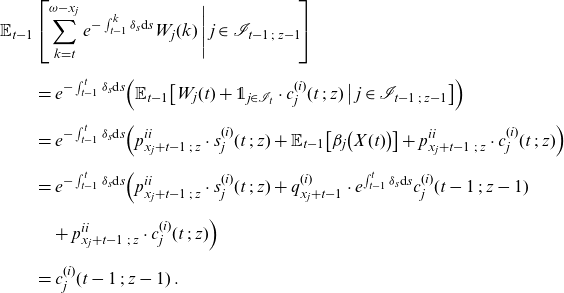 \begin{align*} & \mathbb{E}_{t-1} \left[\sum_{k=t}^{\omega-x_j} e^{- \int_{t-1}^k \delta_s \textrm{d}s} W_j(k) \, \Bigg|\, j \in \mathcal{I}_{t-1\;;\;z-1}\!\right] \\[.2cm]&\qquad = e^{- \int_{t-1}^t \delta_s \textrm{d}s} \Big(\mathbb{E}_{t-1} \big[W_j(t) + \unicode[Times]{x1D7D9}_{j\in\mathcal{I}_t} \cdot c_j^{(i)}(t\;;\;z)\, \big|\, j \in \mathcal{I}_{t-1\;;\;z-1}\big] \Big) \\[.2cm]&\qquad= e^{- \int_{t-1}^t \delta_s \textrm{d}s}\Big(p^{ii}_{x_j+t-1\;;\;z}\cdot s_j^{(i)}(t\;;\;z) + \mathbb{E}_{t-1} \big[\beta_j\big(X(t) \big) \big] + p^{ii}_{x_j+t-1\;;\;z}\cdot c_j^{(i)}(t\;;\;z) \Big) \\[.2cm]&\qquad= e^{- \int_{t-1}^t \delta_s \textrm{d}s}\Big(p^{ii}_{x_j+t-1\;;\;z}\cdot s_j^{(i)}(t\;;\;z) + q^{(i)}_{x_j+t-1}\cdot e^{\int_{t-1}^t \delta_s \textrm{d}s}c_j^{(i)}(t-1\;;\;z-1) \\[.2cm] &\qquad\quad + p^{ii}_{x_j+t-1\;;\;z}\cdot c_j^{(i)}(t\;;\;z) \Big) \\[.2cm]&\qquad= c_j^{(i)}(t-1\;;\;z-1)\,.\end{align*}
This proves (3.22) for
 $t-1$
. For an active person
$t-1$
. For an active person
 $j \in \mathcal{A}_{t-1}$
, we also have that
$j \in \mathcal{A}_{t-1}$
, we also have that
 $c_j^{(a)}(\omega-x_j)=0$
. Using (3.6–3.7), backward iteration enables to obtain:
$c_j^{(a)}(\omega-x_j)=0$
. Using (3.6–3.7), backward iteration enables to obtain:
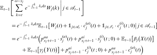 \begin{align*} & \mathbb{E}_{t-1} \Bigg[\sum_{k=t}^{\omega-x_j} e^{- \int_{t-1}^k \delta_s \textrm{d}s} W_j(k) \, \Bigg|\, j \in \mathcal{A}_{t-1} \Bigg] \\[.2cm]&\qquad= e^{- \int_{t-1}^t \delta_s \textrm{d}s} \mathbb{E}_{t-1} \big[W_j(t) + \unicode[Times]{x1D7D9}_{j\in\mathcal{A}_t} \cdot c_j^{(a)}(t) + \unicode[Times]{x1D7D9}_{j\in\mathcal{I}_t} \cdot c_j^{(i)}(t\;;\;0) \big|\, j \in \mathcal{A}_{t-1}\big] \\[.2cm]&\qquad= e^{- \int_{t-1}^t \delta_s \textrm{d}s}\Big(p^{aa}_{x_j+t-1}\cdot s_j^{(a)}(t)+p^{ai}_{x_j+t-1}\cdot s_j^{(i)}(t\;;\;0) + \mathbb{E}_{t-1} \big[\beta_j\big(X(t) \big) \big] \\& \qquad\qquad + \mathbb{E}_{t-1} \big[\gamma_j\big(Y(t) \big) \big] + p^{ai}_{x_j+t-1}\cdot c_j^{(i)}(t\;;\;0) + p^{aa}_{x_j+t-1}\cdot c_j^{(a)}(t) \Big) \end{align*}
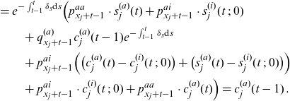 \begin{align*} & \qquad= e^{- \int_{t-1}^t \delta_s \textrm{d}s}\Big(p^{aa}_{x_j+t-1}\cdot s_j^{(a)}(t)+p^{ai}_{x_j+t-1}\cdot s_j^{(i)}(t\;;\;0) \\ & \qquad\qquad + q^{(a)}_{x_j+t-1}c_j^{(a)}(t-1)e^{- \int_{t-1}^t \delta_s \textrm{d}s} \\& \qquad\qquad+p^{ai}_{x_j+t-1}\Big(\big(c_j^{(a)}(t) - c_j^{(i)}(t\;;\;0) \big)+ \big(s_j^{(a)}(t) - s_j^{(i)}(t\;;\;0)\big) \Big) \\& \qquad\qquad + p^{ai}_{x_j+t-1}\cdot c_j^{(i)}(t\;;\;0) + p^{aa}_{x_j+t-1}\cdot c_j^{(a)}(t) \Big) = c_j^{(a)}(t-1)\,.\end{align*}
Appendix C. Proof of Theorem 3.4
For an active person, we can compute the expected value of (3.20) to obtain:
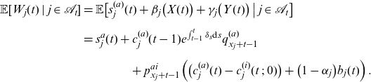 \begin{align}\mathbb{E}[W_j(t)\,|\,j \in \mathcal{A}_{t}] & = \mathbb{E}\big[s_{j}^{(a)}(t)+ \beta_j\big(X(t) \big) + \gamma_j\big(Y(t) \big)\, \big|\, j \in \mathcal{A}_{t}\big] \nonumber\\[5pt]& =s_{j}^a(t) + c_{j}^{(a)}(t-1) e^{\int_{t-1}^t \delta_s \textrm{d}s} q_{x_j+t-1}^{(a)}\nonumber \\[5pt]&\qquad\qquad + p_{x_j+t-1}^{ai} \Big(\big(c_j^{(a)}(t) - c_j^{(i)}(t\;;\;0) \big)+ \big(1-\alpha_j\big) b_j(t) \Big) \,.\end{align}
We use (3.16) to obtain
 $s_j^{(i)}\big(t\;;\;t-T^{(a)}\big)=\alpha_j\cdot \widetilde{s}_j^{\,(i)}(t\;;\;t-T^{(a)})$
for
$s_j^{(i)}\big(t\;;\;t-T^{(a)}\big)=\alpha_j\cdot \widetilde{s}_j^{\,(i)}(t\;;\;t-T^{(a)})$
for
 $t=T^{(a)}+1,$
 $T^{(a)}+2,...$
and for all
$T^{(a)}+2,...$
and for all
 $T^{(a)}$
. We have
$T^{(a)}$
. We have
 \begin{align}c_j^{(i)}(t\;;\;0)=\sum_{u=t+1}^{\omega-x_j} e^{-\int_{t}^u \delta_s \textrm{d}s} s^{(i)}_j(u\;;\;u-t).\end{align}
If survivors want on average an annual payoff of
 $b_j(t)$
, we need to set
$b_j(t)$
, we need to set
 \begin{align*}s_{j}^{(a)}(t) + c_{j}^{(a)}(t-1) e^{\int_{t-1}^t \delta_s \textrm{d}s} q_{x_j+t-1}^{(a)} & + p_{x_j+t-1}^{ai} \Big(\big(c_j^{(a)}(t) - c_j^{(i)}(t\;;\;0) \big) \\ & + \big(1-\alpha_j\big) b_j(t) \Big) = b_j(t)\,.\end{align*}
We can iteratively solve this set of equations backwards in time to obtain (3.26). Equation (3.27) takes into account the immediate increase of benefits at the first payment date after moving into dependency.


 Open access