


1. Introduction
The notion of socio-technical is originally proposed by Trist & Bamforth (Reference Trist and Bamforth1951) in the context of labor studies with the idea that both knowledge accumulation and the improvement of work situations should be embraced in a research project. Over the years, there are two typical types of studies related to the socio-technical concept that can be distinguished. The first type mainly focuses on improving the efficiency of project management (Keating et al. Reference Keating, Fernandez, Jacobs and Kauffmann2001; Hassannezhad et al. Reference Hassannezhad, Cantamessa, Montagna and Clarkson2019). It highlights the complex interactions between the subjective perceptions of workers and the objective characteristics of work processes (Pan & Scarbrough Reference Pan and Scarbrough1998). In the second type, instead of only considering the operation-side actors (employees in firms, researchers, policymakers, etc.), a complete understanding of the human factors within the socio-technical methodology is achieved by taking the demand-side actors (end users, customers, special-interest groups, etc.) into account (Carayon Reference Carayon2006; Geels & Kemp Reference Geels and Kemp2007), but analysing complexity also concurrently increases because of this additional consideration.
When the socio-technical approach is applied to the system development discipline, the term socio-technical system (STS), as an extension of the socio-technical principle and conventional complex systems, is invited. Inheriting the integrative nature of socio-technical concepts, STS combines the social and technical features into the engineering design framework. On the one hand, considering this combination is beneficial because it makes the simulation models and design approaches more consistent to the real situation. On the other hand, it becomes challenging since complexity is introduced by the unpredictable features of the social aspects. This complexity runs through the three broad stages in the system engineering lifecycle: analysis, design and evaluation (Baxter & Sommerville Reference Baxter and Sommerville2011; ElMaraghy et al. Reference ElMaraghy, ElMaraghy, Tomiyama and Monostori2012), and continues to affect the functionality of the entire system. It is also this complexity that raises a high requirement of the system robustness against various disturbances (Kalsi, Hacker, & Lewis Reference Kalsi, Hacker and Lewis1999; Gribble Reference Gribble2001).
One typical disturbance that can impact numerous systems across domains is seasonal effects. Taken the bike-sharing system (BSS) as an example, as shown in Figure 1, seasonal effects not only require the systematic design of station distribution and the capacity of each station to fight against varied weather conditions, but could also generate demand fluctuation in different months that affects BSS’s operational performance. Another example is the electric vehicles that, according to a recent study (Hao et al. Reference Hao, Wang, Lin and Ouyang2020), the electricity consumption of electrical taxis in spring and fall is about 15.2 kWh per 10 km, which is 3.3% and 30% lower than that in summer and winter, respectively. Thus, seasonal effects request that the battery functionality is adaptive to varied climates. Similarly, other systems that can be affected by seasonal changes include power grids, agriculture systems (Ten Napel et al. Reference Ten Napel, Van der Veen, Oosting and Koerkamp2011; Urruty, Tailliez-Lefebvre, & Huyghe Reference Urruty, Tailliez-Lefebvre and Huyghe2016), ecosystems (Ahlström et al. Reference Ahlström, Schurgers, Arneth and Smith2012) and transportation systems (Sun, Wandelt, & Linke Reference Sun, Wandelt and Linke2015; Markolf et al. Reference Markolf, Hoehne, Fraser, Chester and Underwood2019).
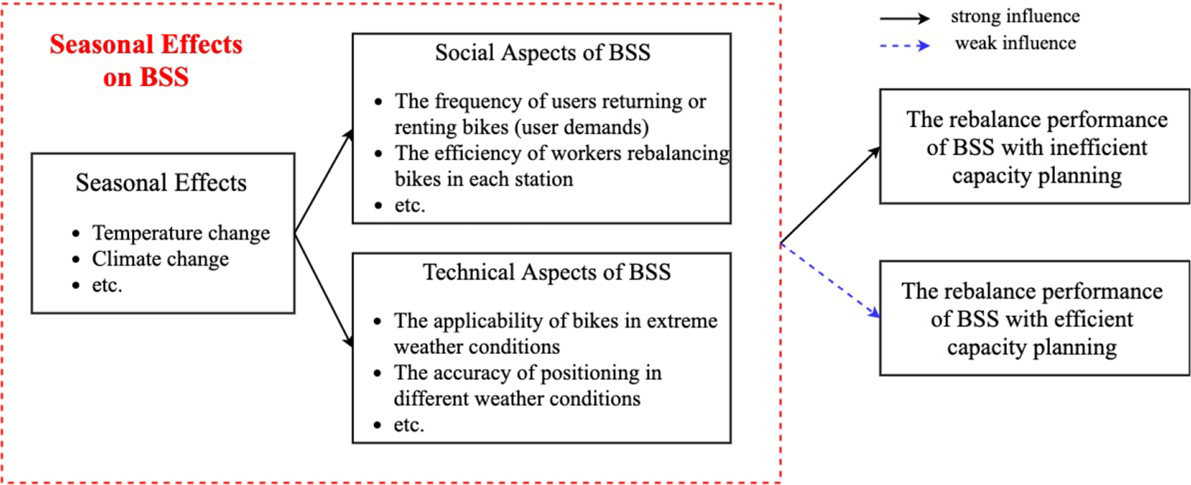
Figure 1. Seasonal effect on bike-sharing system (BSS) with efficient and inefficient capacity planning.
In this paper, we focus on the transportation-based STS where the concept of ‘transportation’ here is much broader than the conventional one. It can refer to the systems that transport passengers and freight such as the air transportation system, and also represents the exchange of information and energy transmission like the interconnected power grids (Blume Reference Blume2017). One common feature of these systems is that they are composed of multiple connected single service subsystems, and each subsystem is designed with certain capacity constrained by resources. Here, the capacity in systems engineering represents the volume of products that a production system generates (Martnez-Costa et al. Reference Martnez-Costa, Mas-Machuca, Benedito and Corominas2014) or the storage capability of physical systems, for example, computing system and warehouses of a supply chain network. It is the capacity planning decision that plays a critical role for the system robustness enhancement of those STSs. Inefficient capacity planning can induce either underutilised resources or unfulfilled user demands, thus leading the system to be sensitive to the seasonal changes. Figure 1 explains how seasonal variations and capacity planning can affect BBS’s performance in more detail. As shown in the figure, the significance of the influence, either negative or positive, is directly related to the number of docks served (i.e., the capacity planned) in each station of such a BSS.
To mitigate the seasonal fluctuation of the STS performance, we propose a new approach to improving the system robustness by optimising capacity planning decisions based on network motif theory. The present study is based on our prior work (Xiao & Sha Reference Xiao and Sha2020) that studies the features of local trip patterns and its correlations to the system-level performance of a BSS using network motifs. In this paper, we further develop a network motif-based framework to support STS robust design in light of seasonal effects. Still, using the bike sharing system as the application context, we show how the the number of docks of critical stations can be optimised to mitigate the seasonal influence on the system’s rebalance performance. This design approach can be generally applied to many other transportation-based STSs where the system robustness against seasonal effects is a primary concern, such as air transportation systems and interconnected power grids.
The remainder of this paper is outlined as follows. Section 2 presents the technical background of the complex network and network motif. In Section 3, we introduce the proposed robust design approach in detail. In Section 4, the application of the approach in BSS is presented and the design problem in terms of capacity planning is formulated. In this section, we also assess the seasonal effect on the BSS’s rebalance performance and discuss the results for capacity planning optimisation. At the end, Section 5 concludes the paper with closing thoughts and directions for future research.
2. Technical background
Complex network is a powerful representation for complex systems because of its ability in capturing the interconnectivity and relationship among the subsystems and individual components. In complex system design and engineering, network science has exhibited its utility in various applications. For example, Sha et al. (Sha, Chaudhari, & Panchal Reference Sha, Chaudhari and Panchal2019; Sha & Panchal Reference Sha and Panchal2013a, Reference Sha and Panchalb; Sha & Panchal Reference Sha and Panchal2016) conducted a broad range of research on network-based engineering design of complex systems including autonomous system level Internet and the U.S. domestic air transportation system. Wang et al. performed a series of studies on applying stochastic network models (e.g., the Exponential Random Graph Model) to model the customer-product interactions in vehicle market systems (Wang et al. Reference Wang, Sha, Huang, Contractor, Fu and Chen2016; Wang et al. Reference Wang, Chen, Huang, Contractor and Fu2016; Fu et al. Reference Fu, Sha, Huang, Wang, Fu and Chen2017; Bi et al. Reference Bi, Xie, Sha, Wang, Fu and Chen2018; Sha et al. Reference Sha, Huang, Fu, Wang, Fu, Contractor and Chen2018; Wang et al. Reference Wang, Sha, Huang, Contractor, Fu and Chen2018; Sha et al. Reference Sha, Bi, Wang, Stathopoulos, Contractor, Fu and Chen2019; Cui et al. Reference Cui, Ahmed, Sha, Wang, Fu and Chen2020). Regarding the network-based robustness analysis, Cats, Koppenol, & Warnier (Reference Cats, Koppenol and Warnier2017) developed a robustness assessment model that can indicate the changes of network performance in different link capacity reductions. This model was successfully applied to public transport systems. In another study, Paparistodimou et al. (Reference Paparistodimou, Duffy, Whitfield, Knight and Robb2020) proposed a network generator to support system architectures’ robustness analysis in the initial design stages. Focusing on design process robustness, Piccolo, Lehmann, & Maier (Reference Piccolo, Lehmann and Maier2018) presented a bipartite network-based method to investigate the interplay between people and the design activities and its impact on the robustness of design progress. These studies validate the feasibility of using complex networks to research STS robustness. It is worth noting that a distinction exists between the concept of robustness in our study and that in the network science literature. The robustness assessments of complex networks focus on evaluating how the removal of nodes, especially the hub nodes, will impact network topologies, for example, a system’s ability to react to failures of its components. However, the robustness defined in this study is investigating whether the nodes with limited capacity can maintain their functions when imbalanced link information is transmitting among nodes. In other words, it indicates system’s ability, relating to each single service component’s capacity planning, to handle the demand fluctuation caused by seasonal effects.
Furthermore, we would like to emphasise the equal importance of both global- and local-level robustness to a system’s operational performance where they respectively indicate the capability of all the service nodes or local clusters of nodes to adapt to the seasonal effects. A better understanding of both of these two levels’ robustness is helpful to guide stakeholders make a tradeoff between the entire system’s performance and subsystems’ functionalities. In this paper, since our focus is more on the robustness investigation of local-level service systems, network motifs – a fundamental local unit of a network (Wang et al. Reference Wang, Peng, Peng, Wang and Chen2020) – is a natural adoption of analysing the local-level system performance.
Network motifs are underlying nonrandom subgraphs within the complex networks. Before named by Milo et al. (Reference Milo, Shen-Orr, Itzkovitz, Kashtan, Chklovskii and Alon2002), network motifs experienced a long research period (Stone, Simberloff, & Artzy-Randrup Reference Stone, Simberloff and Artzy-Randrup2019), which was originally considered as certain patterns statistically emerging in real-world networks instead of the same-sized random networks (Holland & Leinhardt Reference Holland and Leinhardt1974). Since then, motif research can be divided into two main subjects where the first one focuses on motif structure explanation (Alon Reference Alon2007; Paranjape, Benson, & Leskovec Reference Paranjape, Benson and Leskovec2017; Felmlee et al. Reference Felmlee, McMillan, Towsley and Whitaker2018), and the second one is keen on motif mining algorithms (Kashtan et al. Reference Kashtan, Itzkovitz, Milo and Alon2004; Wernicke & Rasche Reference Wernicke and Rasche2006; Choobdar, Ribeiro, & Silva Reference Choobdar, Ribeiro and Silva2012). A motif can be classified as directed or undirected and can also be categorised by the number of nodes it consists of. There are three commonly studied motifs in existing literature, including size-2 motifs (dyads), size-3 motifs (triads) and size-4 motifs (tetrads) (Felmlee et al. Reference Felmlee, McMillan, Towsley and Whitaker2018). As the simplest motifs, dyads are essential to the formation of higher-level motifs and the whole network. Triads, also called ‘transitivity’ motifs, greatly impact the growth of social networks. Tetrads are a newly research focus in recent years, and relevant research comes from a wide range of disciplines, such as biology, electronics and social analysis. Given that the triad is regarded as the foundation in social relationship and the most basic building block of many other complex networks, we decide to adopt size-3 motifs to study STS. Hence, in this paper, only size-3 directed motifs are considered. Their structures and IDs are shown in Table 1 (Rasche & Wernicke Reference Rasche and Wernicke2006).
Table 1. Size-3 directed motif list

The motif IDs determined by Rasche & Wernicke (Reference Rasche and Wernicke2006) consider each motif’s adjacent matrix as a binary representation and transform the binary representation to a decimal number. For example, the binary representation of the decimal number 174 is 010101110, which is consistent with the adjacent matrix of motif 174. Regarding ordering the motifs in Table 1, from top to button and left to right, we rank them based on the number of their arrows from large to small.
There are two common statistics to assess the significance of a network motif in a complex network.
(i) Motif Z-score: Given a graph G and an n-size motif
 $ {G}^{\prime } $
, the frequency of
$ {G}^{\prime } $
, the frequency of
 $ {G}^{\prime } $
in G is the number of times that
$ {G}^{\prime } $
in G is the number of times that
 $ {G}^{\prime } $
appeared in G, which is denoted by
$ {G}^{\prime } $
appeared in G, which is denoted by
 $ {F}_G\left({G}^{\prime}\right) $
. Then, considering an ensemble of random graphs corresponding to the null-model of
$ {F}_G\left({G}^{\prime}\right) $
. Then, considering an ensemble of random graphs corresponding to the null-model of
 $ G $
be
$ G $
be
 $ \Omega (G) $
.
$ \Omega (G) $
.
 $ R(G) $
is a set that includes N randomised networks, all of which are from
$ R(G) $
is a set that includes N randomised networks, all of which are from
 $ \Omega (G) $
. Accordingly, the Z-score is defined as
$ \Omega (G) $
. Accordingly, the Z-score is defined as
 $$ {Z}_G\left({G}^{\prime}\right)=\frac{F_G\left({G}^{\prime}\right)-{u}_R\left({G}^{\prime}\right)}{\sigma_R\left({G}^{\prime}\right)}, $$
where
 $ {u}_R\left({G}^{\prime}\right) $
and
$ {u}_R\left({G}^{\prime}\right) $
and
 $ {\sigma}_R\left({G}^{\prime}\right) $
represent the mean and standard variation of the frequency in
$ {\sigma}_R\left({G}^{\prime}\right) $
represent the mean and standard variation of the frequency in
 $ R(G) $
. In general, a higher Z-score indicates that
$ R(G) $
. In general, a higher Z-score indicates that
 $ {G}^{\prime } $
is a more significant motif in G. Motifs in a larger network may more easily get a higher Z-score than that in a smaller network (Milo et al. Reference Milo, Shen-Orr, Itzkovitz, Kashtan, Chklovskii and Alon2002).
$ {G}^{\prime } $
is a more significant motif in G. Motifs in a larger network may more easily get a higher Z-score than that in a smaller network (Milo et al. Reference Milo, Shen-Orr, Itzkovitz, Kashtan, Chklovskii and Alon2002).
(ii) P-value: P-value indicates the probability of
 $ {F}_r\left({G}^{\prime}\right)>{F}_G\left({G}^{\prime}\right) $
, where
$ {F}_r\left({G}^{\prime}\right)>{F}_G\left({G}^{\prime}\right) $
, where
 $ {F}_r\left({G}^{\prime}\right) $
represents the frequency of
$ {F}_r\left({G}^{\prime}\right) $
represents the frequency of
 $ {G}^{\prime } $
in a random network
$ {G}^{\prime } $
in a random network
 $ r\subset R(G) $
. P-value can be obtained by
$ r\subset R(G) $
. P-value can be obtained by
 $$ {P}_G\left({G}^{\prime}\right)=\frac{1}{N}\sum \limits_{j=1}^N\delta \left({F}_r\left({G}^{\prime}\right)>{F}_G\left({G}^{\prime}\right)\right), $$
where N is the total number of random networks in
 $ R(G) $
. δ is the sign function that equals to 1 when
$ R(G) $
. δ is the sign function that equals to 1 when
 $ {F}_r\left({G}^{\prime}\right)>{F}_G\left({G}^{\prime}\right) $
, and 0 otherwise. Normally, one motif is treated as a significant pattern if its P-value is smaller than a typical level of significance, normally 0.001, 0.01 or 0.05.
$ {F}_r\left({G}^{\prime}\right)>{F}_G\left({G}^{\prime}\right) $
, and 0 otherwise. Normally, one motif is treated as a significant pattern if its P-value is smaller than a typical level of significance, normally 0.001, 0.01 or 0.05.
3. The research approach
In this section, we describe our proposed network motif-based approach in a stepwise framework, as shown in Figure 2.
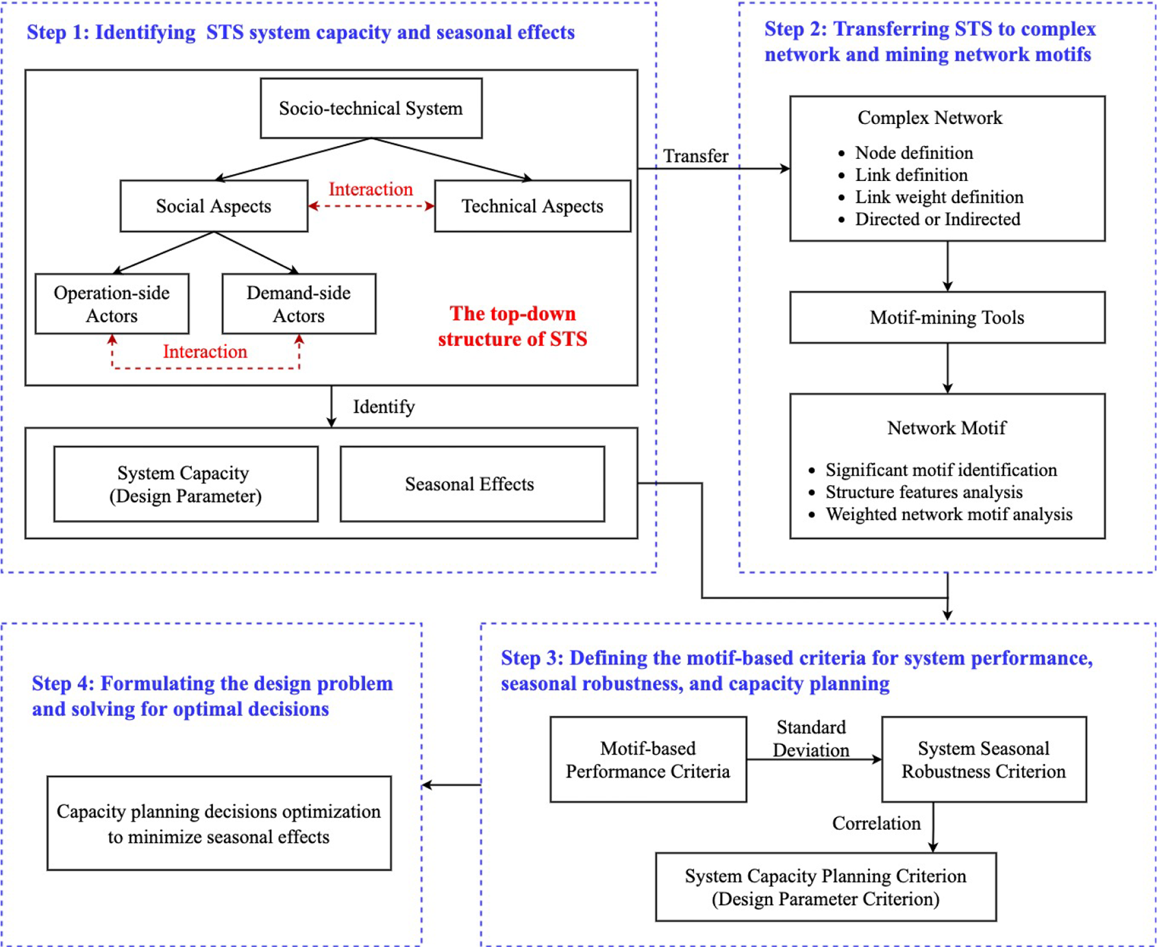
Figure 2. The framework for socio-technical systems (STS) robust design against seasonal effects by capacity planning decisions optimisation.
Step 1: Identifying STS system capacity and seasonal effects
The main objective of this step is to formulate the seasonal robust design problem. It includes understanding the interconnections between different parts (as shown in the top-down structure) within an STS and identifying system capacity and seasonal effects. The in-depth understanding on the system helps lay down the foundation for the complex network construction in Step 2. During this step, data preprocessing is needed to organise the dataset by establishing the preprocessing tenets, for example, data preparation, cleaning, normalisation and transformation of data, and so on (Garca, Luengo, & Herrera Reference Garca, Luengo and Herrera2015).
Step 2: Translating STS to complex network and mining network motifs
Based on the understanding of the target system and the robust design that needs to be addressed, the main tasks in Step 2 are to define and construct the complex network that best captures the STS structures as well as to mine the specific motif patterns in the established network. When building the complex network, we first need to determine the node, node features, link, whether link carries weight or not, weight definition and whether the network is directed or undirected. Secondly, since seasonal data are always time-dependent, two general strategies of handing such a temporal dynamic trait are often used. The first strategy is to treat the year-round data as time-series data, and the second one is to create cross-sectional data at different time steps. Since seasonal information typically changes by month, we adopt the second strategy with the information aggregated from each month. For example, 1 year’s dataset can be divided into 12 cross-sectional datasets, which forms 12 networks denoted as Gi (i = 1,2,…,12).
After the networks are constructed, motif mining tools like FANMOD (Rasche & Wernicke Reference Rasche and Wernicke2006) and Mfinder (Kashtan et al. Reference Kashtan, Itzkovitz, Milo and Alon2002) are employed to enumerate motifs with a particular size in each network. The significance scores (i.e., Z-score and P-value) of each pattern can be obtained at the same time. It is worth noting that during the motif mining, link weights are not used and motif patterns are mined only based on link existence. Link weights can be added latter to the mined motif patterns for analysis if necessary. In our study, if a motif pattern is found significant in all the 12 networks, it is treated as a significant pattern throughout that entire year.
Step 3: Defining the motif-based criteria for system performance, seasonal robustness and capacity planning
Before defining the criteria, we first introduce two node-level performance metrics for directed weighted networks. As shown in Figure 3, assuming a network G has T nodes and for any node
 $ i\subset G $
, there are a incoming weighted links and b outgoing weighted links. We define c as the difference between the sum of incoming link weights and the sum of outgoing link weights. Then, if c = 0, node i is defined as a balanced node; if c < 0, node i is considered to be in-biased node and if c > 0, node i is named out-biased node. This way we are able to quantify a node’s balance performance in STS.
$ i\subset G $
, there are a incoming weighted links and b outgoing weighted links. We define c as the difference between the sum of incoming link weights and the sum of outgoing link weights. Then, if c = 0, node i is defined as a balanced node; if c < 0, node i is considered to be in-biased node and if c > 0, node i is named out-biased node. This way we are able to quantify a node’s balance performance in STS.
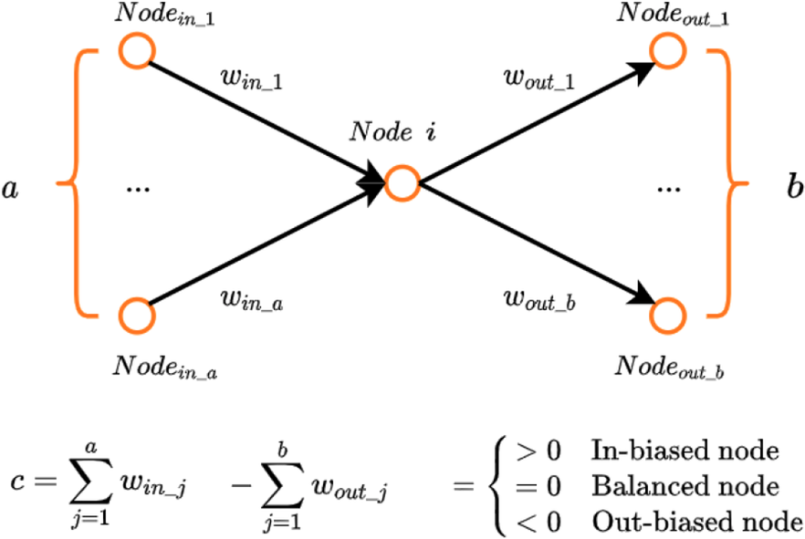
Figure 3. Categorising a node based on its balance performance.
Next, we extend this node classification to network motifs. Supposed there is a size-3 motif comprising three nodes, Node 1, Node 2 and Node 3. A fully connected motif structure is shown in Figure 4. If weight = 0 can be used to represent a nonexistent link (e.g., if w 12 = 0, it means there is no link from Node 1 to Node 2), then all the 13 size-3 directed motifs can be described with the following representation. According to the corresponding c values, Nodes 1, 2 and 3 are divided into three sets: I(m), O(n) and B(l), where m, n and l represent the number of in-biased nodes, out-biased nodes and balanced nodes in each set, and m + n + l = 3 holds. Moreover, the relationship among the three c values follows:
 $$ {c}_1+{c}_2+{c}_3=0. $$

Figure 4. A general motif structure.
Based on these definitions, two metrics, α and β, are created (see Equations (4) and (5)) to grade every single motif in which α depicts the out-biased score and β indicates the in-biased score.
 $$ \alpha =\frac{1}{n}\sum \mid {c}_O\mid, $$
 $$ \beta =\frac{1}{m}\sum \mid {c}_I\mid, $$
where c o or c I indicates the nodes’ c values that falling into the set O(n) or I(m). The higher the scores are, the less balanced is the motif. Based on Equation (3), it can be proved that a linear relation exists between α and β (see Appendix A). The advantages of adopting these two metrics reflect in two aspects. First, they are good indicators of the local-level system performance and can help designers locate the worst performed subpatterns. Second, not only can these two criteria capture the link weights, but they also integrate the topological characteristics of specific motifs.
At the system level, assuming a complex network G consists of K number of motif g (g is the motif ID in Table 1), two motif-based system performance criteria can be obtained below. Similarly,
 $ {\overline{\alpha}}_g $
and
$ {\overline{\alpha}}_g $
and
 $ {\overline{\beta}}_g $
hold a linear relationship, and a higher value indicates a worse balance performance.
$ {\overline{\beta}}_g $
hold a linear relationship, and a higher value indicates a worse balance performance.
 $$ \mathrm{Out}\hbox{-} \mathrm{biased}\ \mathrm{score}:\hskip1em {\overline{\alpha}}_g=\frac{1}{K}\sum \limits_{j=1}^K{\alpha}_{g,j}, $$
 $$ \mathrm{In}\hbox{-} \mathrm{biased}\ \mathrm{score}:\hskip1em {\overline{\beta}}_g=\frac{1}{K}\sum \limits_{j=1}^K{\beta}_{g,j}. $$
Based on the motif-based system performance criteria, the seasonal robustness criterion, as a quantitative representation of the seasonal effect, is defined as the standard deviation of the year-round in- or out-biased score of a motifFootnote
1. For example, according to Step 2, we can get 12 monthly networks
 $ {G}_i $
(
$ {G}_i $
(
 $ i=1,2,\dots, 12 $
) and the yearly significant motif patterns. For each significant motif, its aggregated in- or out-biased score over the 12 consecutive months can be calculated, and the resulting standard deviation from the 12 months, therefore, indicates the system robustness against seasonal changes.
$ i=1,2,\dots, 12 $
) and the yearly significant motif patterns. For each significant motif, its aggregated in- or out-biased score over the 12 consecutive months can be calculated, and the resulting standard deviation from the 12 months, therefore, indicates the system robustness against seasonal changes.
Finally, we define the capacity planning criterion based on the capacity (v) of each service node in a network G. We denote the average capacity difference of a motif as
 $$ d=\frac{\mid {v}_1-{v}_2\mid +\mid {v}_1-{v}_3\mid +\mid {v}_2-{v}_3\mid }{3}, $$
where
 $ {v}_i $
(
$ {v}_i $
(
 $ i=\mathrm{1,2,3} $
) is the capacity of each node i in a size-3 motif. Correspondingly, in the network G consisting of K motif g, the average capacity difference of motif g is
$ i=\mathrm{1,2,3} $
) is the capacity of each node i in a size-3 motif. Correspondingly, in the network G consisting of K motif g, the average capacity difference of motif g is
 $$ {\overline{d}}_g=\frac{1}{K}\sum \limits_{j=1}^K{d}_{g,j}. $$
To provide more insights into how the three motif-based metrics be utilised and extended to different systems, a quick overview of the metric interpretations along with their application examples are summarised in Table 2
Table 2. The interpretations of the metric in different applications
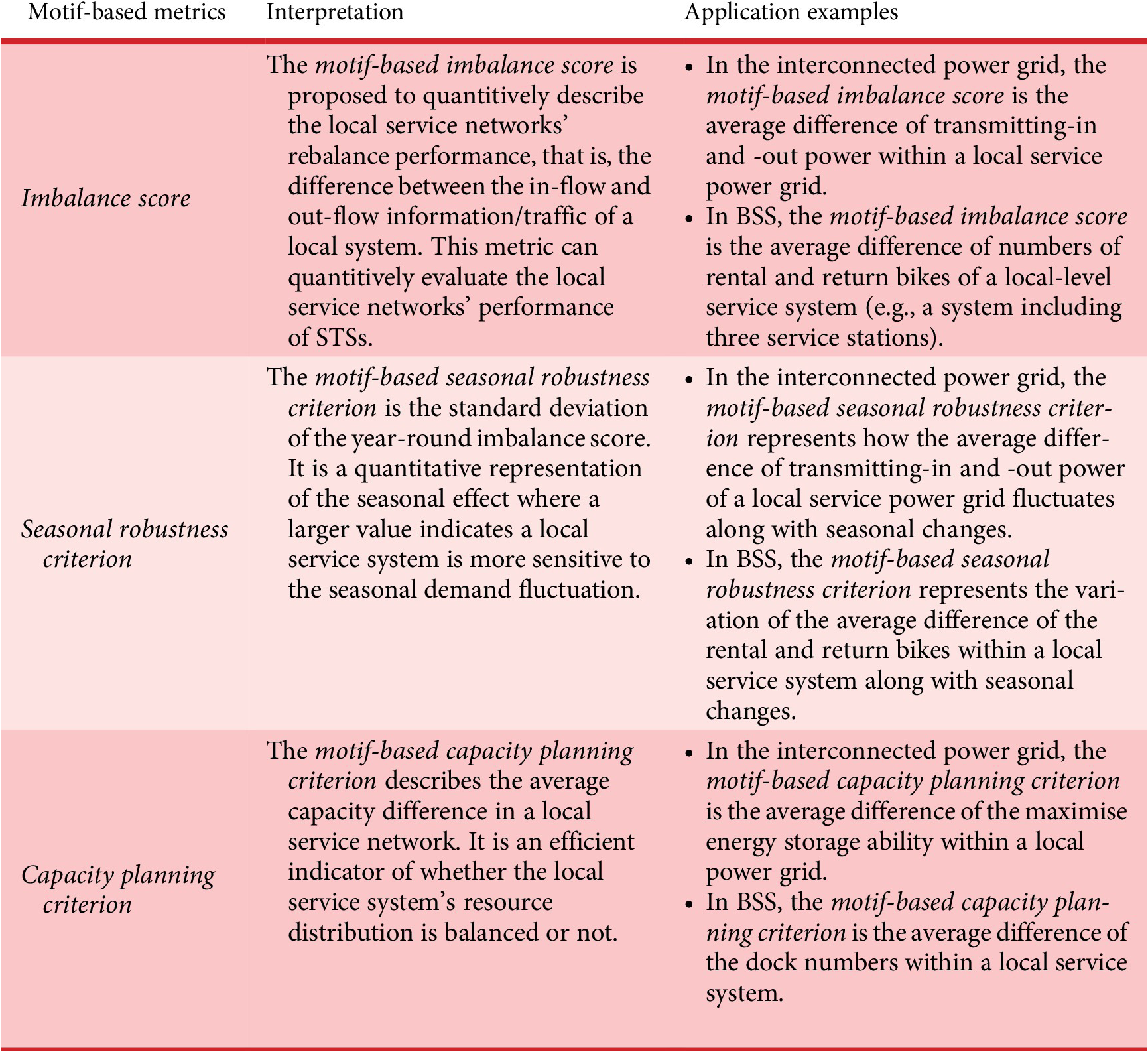
Abbreviations: BSS, bike-sharing system; STS, socio-technical systems.
Step 4: Formulating the design problem and solving for optimal decisions
This step’s objectives are twofold: (i) investigate the correlation between seasonal effects (represented by the seasonal robustness criterion) and the capacity planning criterion, as identified in Step 3 and (ii) formulate the design problem and solve it to obtain optimal decisions for improving the system’s robustness against seasonal disturbance. It would be ideal that the factors influencing the system’s robustness are known from existing domain knowledge, so such factors will be formulated into the design problem as the decision variable to be optimised. Otherwise, correlation analysis and/or causal inference need to be applied to identify the key design variables.
4. Case study
In this study, the Chicago Bike Share program, Divvy Bikes, is selected to demonstrate the proposed approach. The Divvy Bikes’ data is publicly achievable (Divvy_Bike 2020), and the data from 2014 to 2017 are adopted due to the availability of capacity information (i.e., the number of docks) at each station. Figure 5 shows the station distribution of Divvy Bikes in the third and fourth quarters of 2017 and the number of stations in each year. In this study, we aim to mitigate the sensitivity of the system’s rebalance performance to seasonal effects.
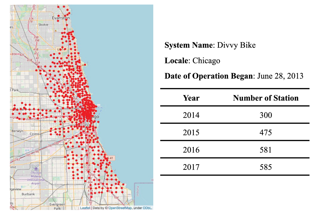
Figure 5. Divvy Bike system information.
4.1. Data preprocessing
The station and trip data packages contain information like station geographic coordinates, the number of docks, trip start and end station IDs, trip time and duration, and user basic information (e.g., gender and birth year). We follow four steps to process the raw data of each year. The final data frame consists of 12 monthly trip datasets, each of which has three columns, including start station ID, end station ID, and the reoccurring frequency of each unique trip.
-
(i) Basic trip information extraction. The essential data, such as the trip start and end station IDs, the number of docks, and start and end times are extracted from the raw dataset.
-
(ii) Data cleaning. We delete those trips with missing data and the the testing stations (e.g., station 512 is a station for testing purpose only) along with their associated trips.
-
(iii) Monthly trip network data preparation. In this step, we split trips by month based on their starting time.
-
(iv) Trip reoccurring frequency calculation. We count the number of times that a trip between a pair of stations occurs in each month.
4.2. Trip network building and motif mining
Based on the monthly trip datasets, the monthly trip networks are constructed. In each network, stations are represented as nodes, and a trip between two stations is defined as a link and its reoccurring frequency in a month is the link weight. Since the trip from Station A to Station B is different from the trip from B to A, the resulting trip network is a directed network.
To focus on the network that captures the most significant traffics, we delete those links that have less occurred trips, such as those links with just one-time transit. The threshold for such a link removal process is set as the minimum mean (u) of the link weights among the 12 monthly trip networks in the interested years:
 $$ u=\mathit{\operatorname{Min}}\left({u}_{ij}\right),i=\mathrm{index}\ \mathrm{of}\ \mathrm{years},\hskip0.5em j=1,2,\dots, 12, $$
where uij is the link weight mean of the jth network in year i. For example, from 2014 to 2017, u = 3.03. Then, all the links with weights lower than 3.03 are removed from the network. Figure 6 illustrates the link weight distribution of Divvy Bikes in July 2017. It reveals that the statistical features of link weights will not be altered by removing the links with weights below the threshold. Figure 7 shows the visualisation of the reduced trip network.
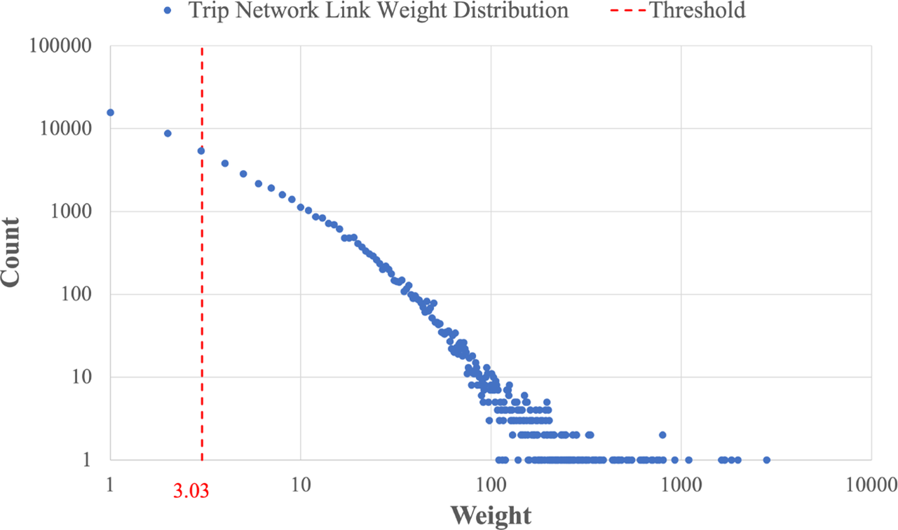
Figure 6. Weight distribution of Divvy Bike trip network (Jul, 2017, total edges: 57,225).

Figure 7. A visualisation of Divvy Bike trip network after removing the links with less occurred trips (Jul, 2017, total edges: 27,415).
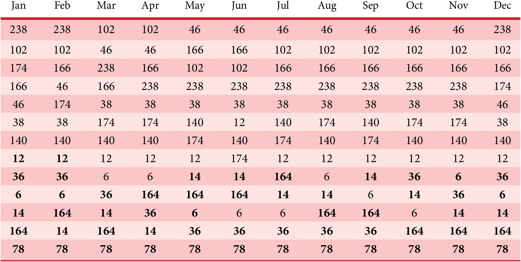
After obtaining the weighted directed trip networks, their binary counterparts (i.e., the same network without link weights) are used for motif mining, which reports the motif structures, Z-scores, P-values, and the adjacent matrix list of all existing motifs. In this study, the motif mining tool FANMOD is adopted. Table 3 shows the 13 size-3 directed motif IDs in every month of 2017, ranked from top to bottom based on their Z-scores from high to low. The bold IDs are insignificant motifs under the level of significance 0.001.
Table 3. Divvy Bike motif Z-score ranks of each month in 2017
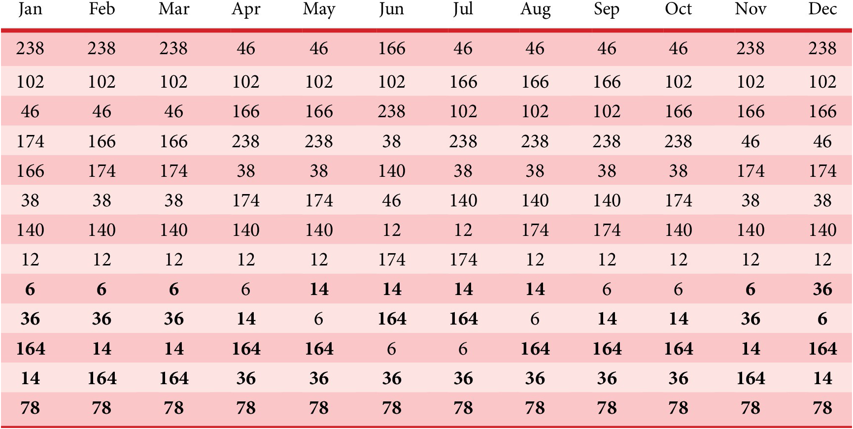
According to the results, we observe that the motifs with high transitivityFootnote 2 are more likely to be significant and ranked higher in the trip network. This is also the reason that motif 78 is always ranked lowest in all networks. The similar phenomenon is also observed in the years from 2014 to 2016, as shown in Appendix B. In the following analysis, only the significant motif patterns in over 2 years, including motifs 238, 102, 174, 166, 38, 46 and 140, are considered.
4.3. Identifying BSS design parameters and seasonal effect
In our prior work (Xiao & Sha Reference Xiao and Sha2020), it is found that seasonal changes can influence the average distances of trip motifs. For example, users tend to ride a longer distance in warmer seasons. Moreover, seasonal changes can impact the traffic of local networks, which is a critical factor to the system rebalance performance. As to the design parameter, based on the correlation analysis (see Table 4), it is found that the number of docks of each station plays an important role in the rebalance problem because it directly relates to the availability of bikes that a user can rent or return in a station.
Table 4. Divvy Bike yearly correlation coefficient between seasonal effect and motif dock differences

Figure 8 shows the average dock difference of those significant motifs in the 12 months of 2017 following Equations (8) and (9). It is observed that the average dock difference curves from top to bottom correspond to the rank of transitivity of the motifs from high to low. For example, motif 238, the pattern with the highest transitivity in the trip networks, has the largest dock difference in the entire year of 2017, while motifs 140 and 38 have the smallest differences. While the causation needs to be further investigated, one possible reason for such a correlation could be that the stations with large capacities are more likely located in high-demand areas, thus more users will return or rent bikes. So, they are hub stations and will connect to many other stations. Meanwhile, there is a majority of stations within the system having low capacities. Therefore, these stations and hubs form a large proportion of motifs with high transitivity and large capacity differences.
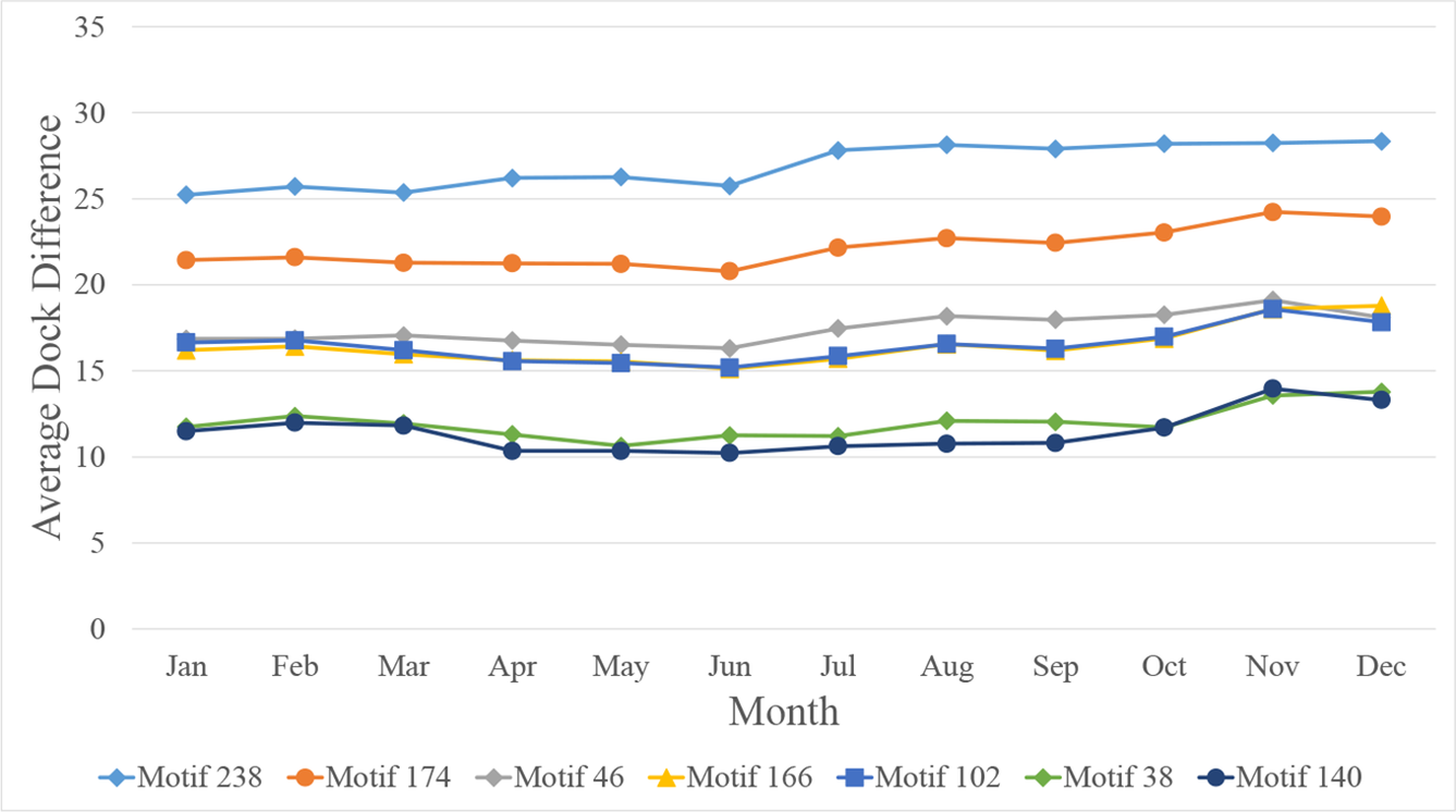
Figure 8. Divvy Bike yearly motif dock difference curves (2017).
4.4. Trip motifs performance and robustness analysis
In this section, by following Step 3 in Section 3, we calculate the local BSS rental and return performance scores, which correspond to the motif-based in- and out-biased values. In a BSS, a higher rental or return score indicates that a serious rebalance issue could occur in a trip motif. Figure 9 shows the rebalance performance scores of the seven significant trip motifs.
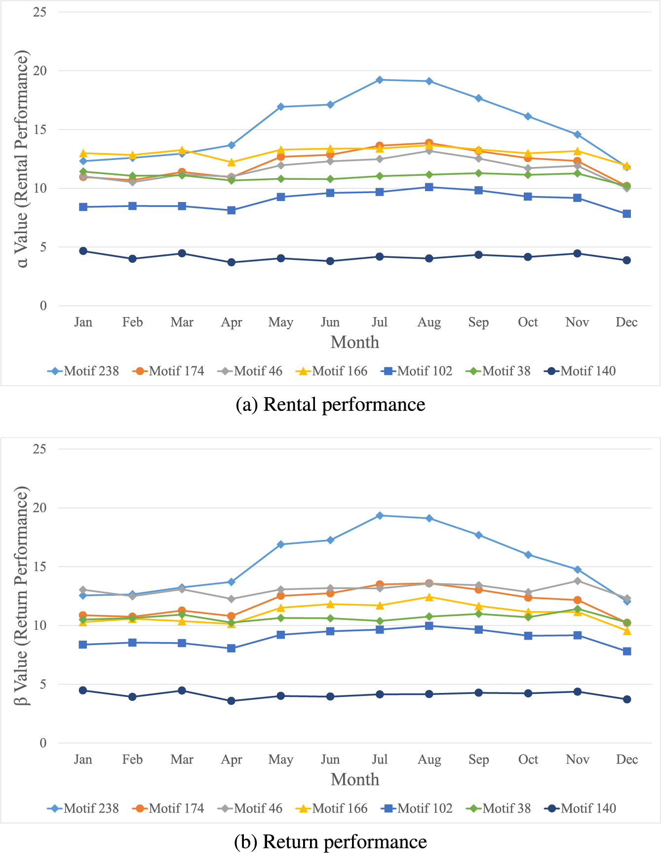
Figure 9. Divvy Bike yearly motif rebalance performance (2017).
As indicated in both Figure 9a,b, the trip motif’s rebalance performance is potentially related to the motif structure. Taken motifs 46, 166 and 140 as examples, both motifs 46 and 166 have apparent unbalanced structures where Node 1 only has in- or out-arrows (see Figure 10). This leads them to be vulnerable to the return and rental problems. In contrast, the number of in- and out-arrows of all nodes in motif 140 are the same, so motif 140 is expected to have a low rebalance performance score. However, there are also a few exceptions. For example, motif 238 has a balanced structure but still experiences return and rental problems in several months from April to November. These abnormal fluctuations remind us of the potential seasonal effects, so we use the standard deviation of the return/rental performance scores in a year to quantify such fluctuations, as shown in the second row of Table 5. A larger deviation means that a trip motif is more sensitive to seasonal changes.
Table 5. Divvy Bike seasonal robustness criteria and capacity planning criteria of significant trip motifs (2017)
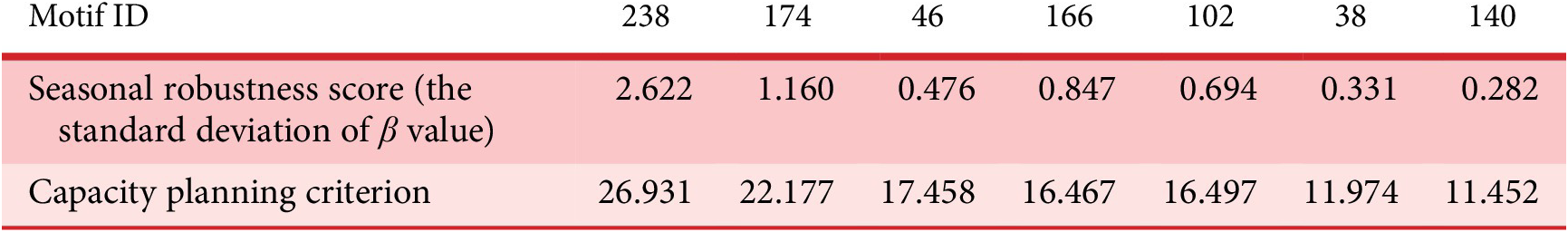

Figure 10. Trip motif structure analysis.
4.5. Design problem formulation
To confirm the targeted design variable, we firstly conducted a correlation analysis between the system robustness and the average capacity difference. Since the robustness score is measured based on yearly data, the mean of the capacity differences of every significant motif during the entire year is calculated, as listed in the third row of Table 5. Based on this table, the correlation coefficient between the system robustness and the capacity planning criterion in 2017 can be obtained, and similarly, for the data from 2014 to 2016.
The results are summarised in Table 4 and reveal a significantly high correlation between the capacity difference and the system’s robustness. In other words, if a trip motif has a large average capacity difference, its rebalance performance would be more sensitive to seasonal changes. This observation has led to our design objective – to optimise the capacity of the stations in the motifs that are most influential to the system’s robustness. To this end, we split the task into two subtasks: (i) identify the stations that need to be optimised for their number of docks and (ii) plan the capacity, that is, the number of docks for those stations, either by adding docks or removing docks, to minimise the average dock difference.
In the first subtask, the motif pattern that is the most sensitive to seasonal changes is chosen (assuming its ID is
 $ {g}_{\mathrm{season}} $
). Then, we determine the objective motifs with the largest dock differences every month and identify the station IDs that construct those motifs. Based on the number of times those identified stations appear in the objective motifs in each month, two decision rulesFootnote
3 are used to decide which stations’ capacity needs to be optimised.
$ {g}_{\mathrm{season}} $
). Then, we determine the objective motifs with the largest dock differences every month and identify the station IDs that construct those motifs. Based on the number of times those identified stations appear in the objective motifs in each month, two decision rulesFootnote
3 are used to decide which stations’ capacity needs to be optimised.
-
(i) The first rule is that among all 12 months, if a station appears in the most number of months, then it will be regarded as the critical station and its capacity will be taken into account for optimisation. From the first rule, we will identify a set of critical stations, S 1.
-
(ii) In the second rule, the stations appearing most frequently in each month are chosen as critical stations, and the corresponding station set is defined as S 2. Finally, we define all the critical stations being represented as
 $ S={S}_1\cup \hskip0.2em {S}_2 $
.
$ S={S}_1\cup \hskip0.2em {S}_2 $
.

In the second subtask, assuming the significant motif set is M, including m different types of motifs, we identify the significant motifs (from M) in which a critical station s (
 $ s\in S $
) appears, and put the same type of motifs with the ID
$ s\in S $
) appears, and put the same type of motifs with the ID
 $ g\in M $
in one set,
$ g\in M $
in one set,
 $ {M}_{s,g} $
. Next, we define the decision variable xs as the number of docks that station s need to add (
$ {M}_{s,g} $
. Next, we define the decision variable xs as the number of docks that station s need to add (
 $ {x}_s>0 $
) or remove (
$ {x}_s>0 $
) or remove (
 $ {x}_s<0 $
). Then, the updated average capacity difference of the motif g,
$ {x}_s<0 $
). Then, the updated average capacity difference of the motif g,
 $ {d}_{s,g,j} $
, can be calculated by following Equation (11), where s
1, s
2 and s
3 represent three stations’ IDs in a motif. Depending on whether s
1, s
2 and s
3 belong to the critical station set S or not,
$ {d}_{s,g,j} $
, can be calculated by following Equation (11), where s
1, s
2 and s
3 represent three stations’ IDs in a motif. Depending on whether s
1, s
2 and s
3 belong to the critical station set S or not,
 $ {d}_{s,g,j} $
is calculated differently.
$ {d}_{s,g,j} $
is calculated differently.
 $$ \left\{\begin{array}{ll}\begin{array}{l}{d}_{s,g,j}\left({x}_{s_1}\right)=\frac{1}{3}\Big[\mid \left({v}_{s_1}+{x}_{s_1}\right)-{v}_2\mid \\ {}\hskip7.48em +\mid \left({v}_{s_1}+{x}_{s_1}\right)-{v}_3\mid +\mid {v}_2-{v}_3\mid \Big]\end{array}& \mathrm{if}\;{s}_1\in S\\ {}\begin{array}{l}{d}_{s,g,j}\left({x}_{s_1},{x}_{s_2}\right)=\frac{1}{3}\Big[\mid \left({v}_{s_1}+{x}_{s_1}\right)-\left({v}_{s_2}+{x}_{s_2}\right)\mid \\ {}\hskip9.8em +\mid \left({v}_{s_1}+{x}_{s_1}\right)-{v}_3\mid +\mid \left({v}_{s_2}+{x}_{s_2}\right)-{v}_3\mid \Big]\end{array}& \mathrm{if}\;{s}_1,{s}_2\in S\\ {}\begin{array}{l}{d}_{s,g,j}\left({x}_{s_1},{x}_{s_2},{x}_{s_3}\right)=\frac{1}{3}\Big[\mid \left({v}_{s_1}+{x}_{s_1}\right)-\left({v}_{s_2}+{x}_{s_2}\right)\mid \\ {}\hskip12em +\mid \left({v}_{s_1}+{x}_{s_1}\right)-\left({v}_{s_3}+{x}_{s_3}\right)\mid \\ {}\hskip12em +\mid \left({v}_{s_2}+{x}_{s_2}\right)-\left({v}_{s_3}+{x}_{s_3}\right)\mid \Big]\end{array}& \mathrm{if}\;{s}_1,{s}_2,{s}_3\in S\end{array}\right. $$
Finally, the updated average dock difference for motifs in set
 $ {M}_{s,g} $
can be obtained
$ {M}_{s,g} $
can be obtained
 $$ {\overline{d}}_{s,g}=\frac{1}{m_{s,g}}\sum \limits_{j=1}^{m_{s,g}}{d}_{s,g,j}, $$
where
 $ {m}_{s,g} $
is the number of motifs in
$ {m}_{s,g} $
is the number of motifs in
 $ {M}_{s,g} $
.
$ {M}_{s,g} $
.
Since the objective is to minimise the average dock difference of those identified trip motifs, a multiobjective optimisation is formulated in Equation (13):
 $$ {\displaystyle \begin{array}{l}\left\{\begin{array}{l}\min {\overline{d}}_{s_1,{g}_1}=\min \frac{1}{m_{s_1,{g}_1}}{\sum}_{j=1}^{m_{s_1,{g}_1}}{d}_{s_1,{g}_1,j}\\ {}\dots \\ {}\min {\overline{d}}_{s_1,{g}_m}=\min \frac{1}{m_{s_1,{g}_m}}{\sum}_{j=1}^{m_{s_1,{g}_m}}{d}_{s_1,{g}_m,j}\\ {}\dots \\ {}\min {\overline{d}}_{s_l,{g}_1}=\min \frac{1}{m_{s_l,{g}_1}}{\sum}_{j=1}^{m_{s_l,{g}_1}}{d}_{s_l,{g}_1,j}\\ {}\dots \\ {}\min {\overline{d}}_{s_l,{g}_m}=\min \frac{1}{m_{s_l,{g}_m}}{\sum}_{j=1}^{m_{s_l,{g}_m}}{d}_{s_l,{g}_m,j}\end{array}\right.\\ {}\mathrm{S}.\mathrm{T}.\hskip0.4em {x}_{s_1}\ge -{v}_{s_1},\dots, {x}_{s_l}\ge -{v}_{s_l}\hskip0.4em \mathrm{and}\hskip0.4em {x}_{s_1},\dots, {x}_{s_l}\in \hskip0.2em \boldsymbol{Z},\end{array}} $$
where
 $ {s}_1,\dots, {s}_l\in S $
,
$ {s}_1,\dots, {s}_l\in S $
,
 $ {g}_1,\dots, {g}_m\in M $
and
$ {g}_1,\dots, {g}_m\in M $
and
 $ {v}_{s_1},\dots, {v}_{s_l} $
are the original dock numbers of station
$ {v}_{s_1},\dots, {v}_{s_l} $
are the original dock numbers of station
 $ {s}_1,\dots, {s}_l $
.
Z
denotes Integer. In Equation (13), all the relevant motifs in M, even if they are not
$ {s}_1,\dots, {s}_l $
.
Z
denotes Integer. In Equation (13), all the relevant motifs in M, even if they are not
 $ {g}_{\mathrm{season}} $
, are considered. This is because while we are changing the number of docks for those stations in motif
$ {g}_{\mathrm{season}} $
, are considered. This is because while we are changing the number of docks for those stations in motif
 $ {g}_{\mathrm{season}} $
, there is a possibility that the average dock difference in the other motifs which include the stations of
$ {g}_{\mathrm{season}} $
, there is a possibility that the average dock difference in the other motifs which include the stations of
 $ {g}_{\mathrm{season}} $
increases too.
$ {g}_{\mathrm{season}} $
increases too.
To solve this optimisation problem, we adopt the weighting method (Miettinen Reference Miettinen2012) to transform the multiobjective optimisation problem to a single-objective one in Equation (14). Suppose all objective functions in Equation (13) are equally important, and
 $ {\sum}_{i=1}^{m\times l}{q}_i=1 $
, then
$ {\sum}_{i=1}^{m\times l}{q}_i=1 $
, then
 $ {q}_i=q=\frac{1}{m\times l} $
(
$ {q}_i=q=\frac{1}{m\times l} $
(
 $ i=1,\dots, m\times l $
). Equation (14) is a typical nonlinear integer optimisation problem, and the genetic algorithm, ga function in MATLAB (2020) is applied to solve this problem.
$ i=1,\dots, m\times l $
). Equation (14) is a typical nonlinear integer optimisation problem, and the genetic algorithm, ga function in MATLAB (2020) is applied to solve this problem.
 $$ {\displaystyle \begin{array}{ll}\min D\Big({x}_{s_1}, \dots, {x}_{s_l}\Big)=\min \left[q\left({\overline{d}}_{s_1,{g}_1}+{\overline{d}}_{s_1,{g}_m}+\dots +{\overline{d}}_{s_l,{g}_1}+{\overline{d}}_{s_l,{g}_m}\right)\right],\\ {}\mathrm{S}.\mathrm{T}.\hskip0.4em {x}_{s_1}\ge -{v}_{s_1},\dots, {x}_{s_l}\ge -{v}_{s_l}\hskip0.4em \mathrm{and}\hskip0.4em {x}_{s_1},\dots, {x}_{s_l}\in \hskip0.2em \boldsymbol{Z},\end{array}} $$
In our case study, based on Figure 9, we identify
 $ M=\left\{\mathrm{238,174,46,166,102,38,140}\right\} $
and motif 238 is the target motif we need to focus on because it is the most sensitive one in light of seasonal changes. Table 6 lists all the critical stations which form motif 238 and yield the largest dock difference. From Table 6, we can observe that, station 3, the most frequently appeared station (9 months out of 12), should be considered as a critical station, that is,
$ M=\left\{\mathrm{238,174,46,166,102,38,140}\right\} $
and motif 238 is the target motif we need to focus on because it is the most sensitive one in light of seasonal changes. Table 6 lists all the critical stations which form motif 238 and yield the largest dock difference. From Table 6, we can observe that, station 3, the most frequently appeared station (9 months out of 12), should be considered as a critical station, that is,
 $ {S}_1=\left\{3\right\} $
. Regarding the stations that appear most in each month, taking March as an example, we identified 15 critical motif 238s, and station 35 and 172 are the most frequently appeared stations in all of the 15 critical motifs. Thus, they are considered as critical stations. Similarly, another four critical stations are identified, thus
$ {S}_1=\left\{3\right\} $
. Regarding the stations that appear most in each month, taking March as an example, we identified 15 critical motif 238s, and station 35 and 172 are the most frequently appeared stations in all of the 15 critical motifs. Thus, they are considered as critical stations. Similarly, another four critical stations are identified, thus
 $ {S}_2=\left\{\mathrm{3,35,45,97,172,263}\right\} $
. By combining these two sets, we obtain the final critical station set
$ {S}_2=\left\{\mathrm{3,35,45,97,172,263}\right\} $
. By combining these two sets, we obtain the final critical station set
 $ S={S}_1\cup {S}_2=\left\{\mathrm{3,35,45,97,172,263}\right\} $
.
$ S={S}_1\cup {S}_2=\left\{\mathrm{3,35,45,97,172,263}\right\} $
.
Table 6. Station list of constructing the motif 238s with the largest dock difference values
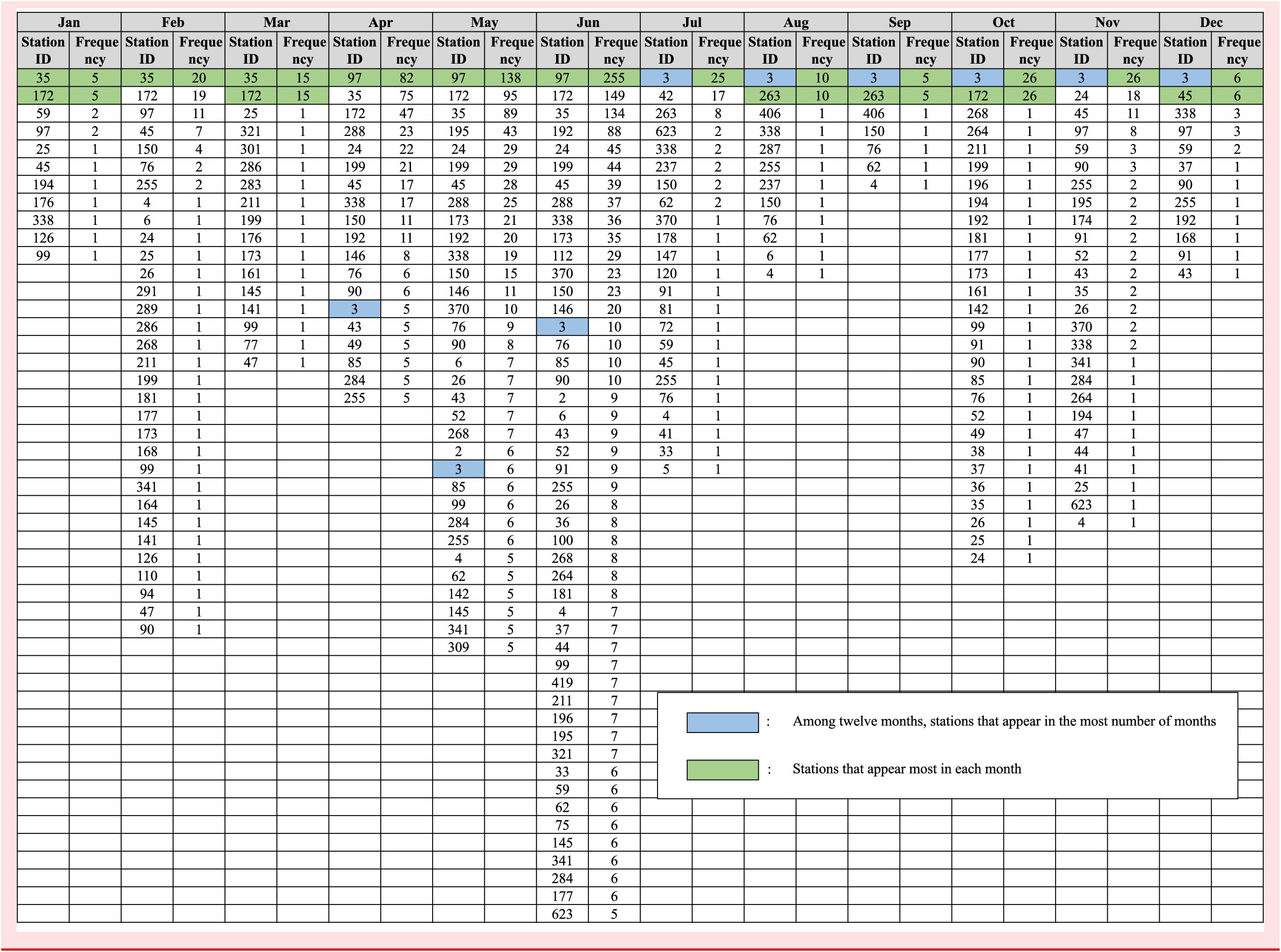
Due to the space limitation, stations with appearing frequencies less than 5 in April, May and June are ignored, and this ignorance has no effect on critical station identification.
By solving the optimisation problem in Equation (14), we obtain the optimal capacity planning decision for the decision variables
 $ {x}_{s_1} $
,…,
$ {x}_{s_1} $
,…,
 $ {x}_{s_6} $
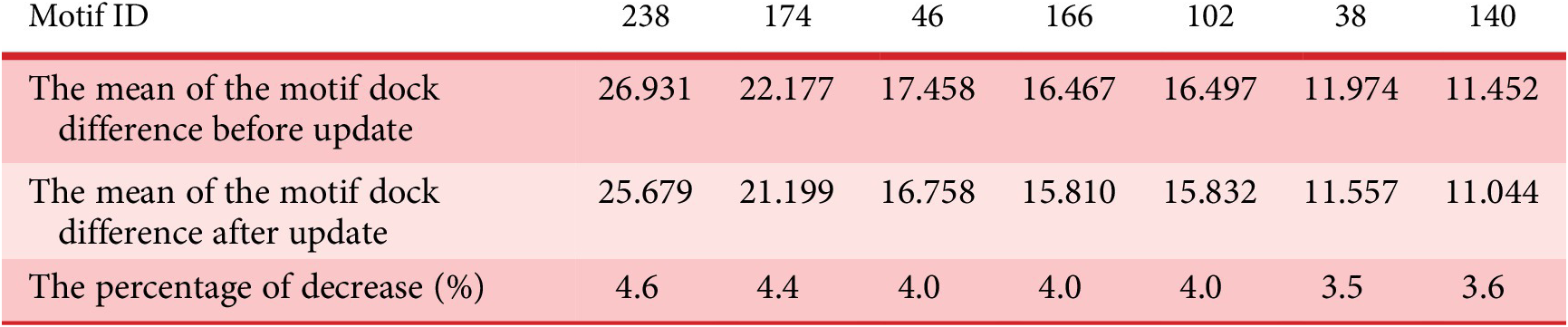
. The results are shown in Table 7, along with the original and updated number of docks. To verify if the redesigned capacity can effectively decrease the average dock difference of the significant trip motifs or not, we recalculate the trip motifs’ mean values of the updated number of docks in a year, as shown in Table 8. By comparing the updated dock differences with the original ones, it is found that the decreases are achieved for all significant motifs, and the dock difference of motif 238 is decreased by 4.6%. With such a decrease, the enhance of the system robustness against seasonal effects is expected to be achieved effectively.
$ {x}_{s_6} $
. The results are shown in Table 7, along with the original and updated number of docks. To verify if the redesigned capacity can effectively decrease the average dock difference of the significant trip motifs or not, we recalculate the trip motifs’ mean values of the updated number of docks in a year, as shown in Table 8. By comparing the updated dock differences with the original ones, it is found that the decreases are achieved for all significant motifs, and the dock difference of motif 238 is decreased by 4.6%. With such a decrease, the enhance of the system robustness against seasonal effects is expected to be achieved effectively.


Table 8. Divvy Bike yearly mean values of significant motif dock differences, before update versus after update (2017)
5. Conclusion
It is the uncertainty and complicated interactions within an STS that make the system vulnerable to various perturbations. The occurrence of certain perturbations can significantly influence the STS performance, and the seasonal effect is a common one because it directly impacts human behaviour in STS. In this study, we develop a new design framework for improving STS robustness against seasonal changes based on the network motif theory. Using the concepts of motif, we created three metrics for system performance evaluation and capacity planning decision-making. The first one is the imbalance score of a motif (e.g., a local service network), the second one is the measurement of a motif’s seasonal robustness, and the third one is a design parameter-based capacity planning decision criterion. We apply our developed approach to a real-world STS, Divvy Bikes, a Chicago Bike Share program, to improve the system’s rebalance performance and its robustness against seasonal changes. The results from this study show that our approach can effectively reduce the average dock differences among the stations of critical trip motifs (i.e., local trip networks), thereby improving the system’s robustness.
The main contributions of this paper are summarised in three aspects: (i) We introduce a network motif-based approach for guiding the STS robust design, emphasising optimising system capacity planning to weaken the impact from demand fluctuations caused by seasonal changes. (ii) We propose a set of motif-based criteria to help evaluate system’s performance and the impact of seasonal effects on it. (iii) High correlation between the seasonal effects and the average dock difference of motifs is discovered in BSS, from which a multiobjective design problem is formulated to aid capacity planning decisions for improved system robustness.
There are two limitations in this study. First, in the STS robustness analysis, only seasonal effects are considered. However, in reality, it is common that several types of disturbances, such as the explicit interaction of BSS with other public transportation systems and varying population growth in different areas, could co-exist and influence a system’s performance in a more unpredictable and dynamic manner. Second, in the robust design, it is expected to have a predictive model for the trip network so that after docks are added or removed at the critical stations, the resulting imbalance scores can be updated and the local trip networks’ performance can be re-evaluated to further verify the effectiveness of the design solutions. Taking this work as a starting point, we would like to develop a dynamic approach, in conjunction with the temporal motif concept, to support STS short-term robustness analysis. In this case, more temporal uncertainties, such as varying demands at different periods of a day or system self-rebalancing strategy (e.g., bike-sharing company utilising trucks to rebalance the number of bikes in different stations), will be considered. Furthermore, we would also like to pursue a more comprehensive framework to guide the robust design of complex STS by taking into account more influence disturbances.
Appendix A. Validating the linear relationship between α and β
Based on Equation (3), all the possible calculation of α and β, depending on whether c values are larger than 0 or not, are enumerated as follows:
(i) If
 $ {c}_1>0 $
,
$ {c}_1>0 $
,
 $ {c}_2<0 $
, and
$ {c}_2<0 $
, and
 $ {c}_3<0 $
:
$ {c}_3<0 $
:
 $$ \beta ={c}_1,\hskip1em \alpha =\frac{1}{2}\mid {c}_2+{c}_3\mid, $$
 $$ \mathrm{So},\hskip1em \beta =2\alpha . $$
Similar relationship can be achieved when
 $ {c}_2>0 $
,
$ {c}_2>0 $
,
 $ {c}_1<0 $
and
$ {c}_1<0 $
and
 $ {c}_3<0 $
or
$ {c}_3<0 $
or
 $ {c}_3>0 $
,
$ {c}_3>0 $
,
 $ {c}_1<0 $
and
$ {c}_1<0 $
and
 $ {c}_2<0 $
.
$ {c}_2<0 $
.
(ii) If
 $ {c}_1>0 $
,
$ {c}_1>0 $
,
 $ {c}_2>0 $
, and
$ {c}_2>0 $
, and
 $ {c}_3<0 $
:
$ {c}_3<0 $
:
 $$ \beta =\frac{1}{2}\left({c}_1+{c}_2\right),\hskip1em \alpha =\mid {c}_3\mid, $$
 $$ \mathrm{So},\hskip1em \beta =\frac{1}{2}\alpha . $$
Similar relationship can be achieved when
 $ {c}_1>0 $
,
$ {c}_1>0 $
,
 $ {c}_3>0 $
and
$ {c}_3>0 $
and
 $ {c}_2<0 $
or
$ {c}_2<0 $
or
 $ {c}_2>0 $
,
$ {c}_2>0 $
,
 $ {c}_3>0 $
and
$ {c}_3>0 $
and
 $ {c}_1<0 $
.
$ {c}_1<0 $
.
(iii) If
 $ {c}_1=0 $
,
$ {c}_1=0 $
,
 $ {c}_2>0\left(<0\right) $
and
$ {c}_2>0\left(<0\right) $
and
 $ {c}_3<0\left(>0\right) $
:
$ {c}_3<0\left(>0\right) $
:
 $$ \beta ={c}_2,\hskip1em \alpha =\mid {c}_3\mid, $$
 $$ \mathrm{So},\hskip1em \beta =\alpha . $$
Similar relationship can be achieved when
 $ {c}_1>0\left(<0\right) $
,
$ {c}_1>0\left(<0\right) $
,
 $ {c}_2=0 $
and
$ {c}_2=0 $
and
 $ {c}_3<0\left(>0\right) $
or
$ {c}_3<0\left(>0\right) $
or
 $ {c}_1>0\left(<0\right) $
,
$ {c}_1>0\left(<0\right) $
,
 $ {c}_2<0\left(>0\right) $
and
$ {c}_2<0\left(>0\right) $
and
 $ {c}_3=0 $
.
$ {c}_3=0 $
.
(iv) If
 $ {c}_1=0 $
,
$ {c}_1=0 $
,
 $ {c}_2=0 $
and
$ {c}_2=0 $
and
 $ {c}_3=0 $
:
$ {c}_3=0 $
:
 $$ \beta =\alpha =0. $$
Therefore, the linear relationship between α and β is validated.
Appendix B. Divvy Bike motif Z-score ranks in 2014–2016
From Table B1 to Table B3, the same trend described in Section 4.2 is further verified that the motifs with higher transitivity are more likely to be significant. This is also the reason that motif 238 and 46 are always ranked highest while motif 78 lowest in almost all networks.
Table B1. Divvy Bike motif Z-score ranks of each month in 2014
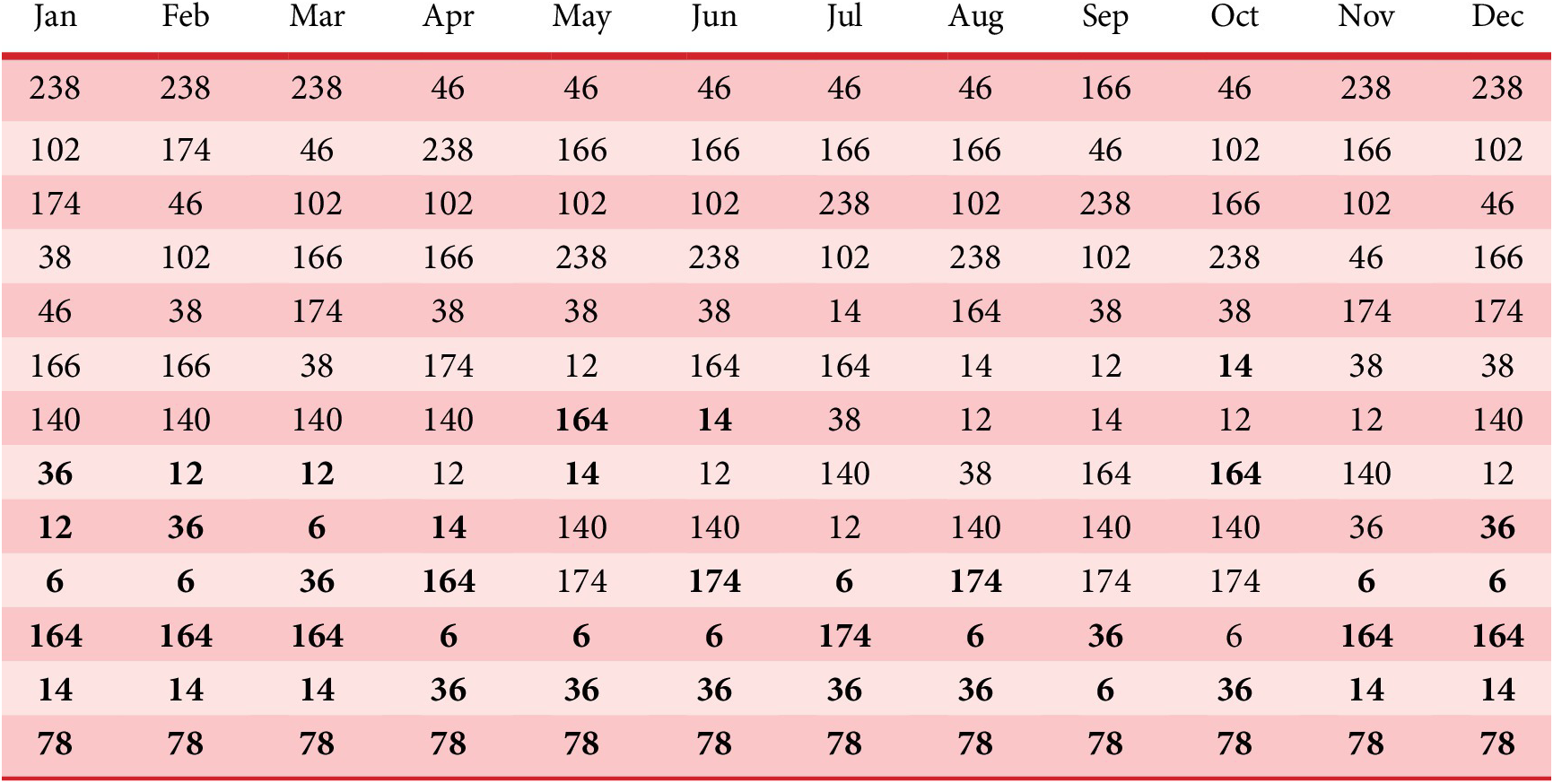
Table B2. Divvy Bike motif Z-score ranks of each month in 2015

Table B3. Divvy Bike motif Z-score ranks of each month in 2016


 Open access