


1 Introduction: dimensions of self-affine measures
Let
 $\nu $
be a compactly supported Borel probability measure in
$\nu $
be a compactly supported Borel probability measure in
 $\mathbb {R}^d$
. The Assouad and lower dimensions of
$\mathbb {R}^d$
. The Assouad and lower dimensions of
 $\nu $
quantify the extremal local fluctuations of the measure by considering the relative measure of concentric balls. In particular, a measure is doubling if and only if it has finite Assouad dimension; see, for example, [Reference Fraser11, Lemma 4.1.1]. Write
$\nu $
quantify the extremal local fluctuations of the measure by considering the relative measure of concentric balls. In particular, a measure is doubling if and only if it has finite Assouad dimension; see, for example, [Reference Fraser11, Lemma 4.1.1]. Write
 $\mathrm {supp}(\nu )$
to denote the support of
$\mathrm {supp}(\nu )$
to denote the support of
 $\nu $
and
$\nu $
and
 $|F|$
to denote the diameter of a non-empty set F. The Assouad dimension of
$|F|$
to denote the diameter of a non-empty set F. The Assouad dimension of
 $\nu $
is defined by
$\nu $
is defined by
 $$ \begin{align*} \dim_{\mathrm{A}} \nu=\inf \bigg\{s \geqslant 0: &\text{ there exists } C>0 \text{ such that, for all } x \in \mathrm{supp}(\nu) \\ &\text{ and for all } 0<r<R<|\mathrm{supp}(\nu)|, \frac{\nu(B(x, R))}{\nu(B(x, r))} \leqslant C\bigg(\frac{R}{r}\bigg)^{s}\bigg\}, \end{align*} $$
and, provided
 $|\mathrm {supp}(\nu )|>0$
, the lower dimension of
$|\mathrm {supp}(\nu )|>0$
, the lower dimension of
 $\nu $
is
$\nu $
is
 $$ \begin{align*} \dim_{\mathrm{L}} \nu=\sup \bigg\{s \geqslant 0: &\text{ there exists } C>0 \text{ such that, for all } x \in \mathrm{supp}(\nu) \\ &\text{ and for all } 0<r<R<|\mathrm{supp}(\nu)|, \frac{\nu(B(x, R))}{\nu(B(x, r))} \geqslant C\bigg(\frac{R}{r}\bigg)^{s}\bigg\}. \end{align*} $$
If
 $|\mathrm {supp}(\nu )|=0$
, then
$|\mathrm {supp}(\nu )|=0$
, then
 $\dim _{\mathrm {L}} \nu =0$
. The Assouad and lower dimensions of measures were introduced by Käenmäki, Lehrbäck and Vuorinen [Reference Käenmäki, Lehrbäck and Vuorinen15], where they were originally referred to as the upper and lower regularity dimensions, respectively. We are interested in the Assouad and lower dimensions of self-affine measures.
$\dim _{\mathrm {L}} \nu =0$
. The Assouad and lower dimensions of measures were introduced by Käenmäki, Lehrbäck and Vuorinen [Reference Käenmäki, Lehrbäck and Vuorinen15], where they were originally referred to as the upper and lower regularity dimensions, respectively. We are interested in the Assouad and lower dimensions of self-affine measures.
Given a finite index set
 $\mathcal {I}=\{1,\ldots ,N\}$
, an affine iterated function system (IFS) on
$\mathcal {I}=\{1,\ldots ,N\}$
, an affine iterated function system (IFS) on
 $\mathbb {R}^d$
is a finite family
$\mathbb {R}^d$
is a finite family
 $\mathcal {F}=\{f_i\}_{i\in \mathcal {I}}$
of affine contracting maps
$\mathcal {F}=\{f_i\}_{i\in \mathcal {I}}$
of affine contracting maps
 $f_i(x)=A_i x+t_i$
. The IFS determines a unique, non-empty compact set F, called the attractor, which satisfies the relation
$f_i(x)=A_i x+t_i$
. The IFS determines a unique, non-empty compact set F, called the attractor, which satisfies the relation
 $$ \begin{align*} F = \bigcup_{i\in\mathcal{I}} f_i(F). \end{align*} $$
Given a probability vector
 $\mathbf {p}=(p(i))_{i\in \mathcal {I}}$
with strictly positive entries, the self-affine measure
$\mathbf {p}=(p(i))_{i\in \mathcal {I}}$
with strictly positive entries, the self-affine measure
 $\nu _{\mathbf {p}}$
fully supported on F is the unique Borel probability measure
$\nu _{\mathbf {p}}$
fully supported on F is the unique Borel probability measure
 $$ \begin{align*} \nu_{\mathbf{p}} = \sum_{i\in\mathcal{I}} p(i)\, \nu_{\mathbf{p}}\circ f_i^{-1}. \end{align*} $$
The measure
 $\nu _{\mathbf {p}} $
has an equivalent characterization as the pushforward of the Bernoulli measure generated by
$\nu _{\mathbf {p}} $
has an equivalent characterization as the pushforward of the Bernoulli measure generated by
 $\mathbf {p}$
under the natural projection from the symbolic space to the attractor. More precisely, given
$\mathbf {p}$
under the natural projection from the symbolic space to the attractor. More precisely, given
 $\mathbf {p}$
, the Bernoulli measure on the symbolic space
$\mathbf {p}$
, the Bernoulli measure on the symbolic space
 $\Sigma =\mathcal {I}^{\mathbb {N}}$
is the product measure
$\Sigma =\mathcal {I}^{\mathbb {N}}$
is the product measure
 $\mu _{\mathbf {p}}=\mathbf {p}^{\mathbb {N}}$
. The natural projection
$\mu _{\mathbf {p}}=\mathbf {p}^{\mathbb {N}}$
. The natural projection
 $\pi :\Sigma \to F$
is given by
$\pi :\Sigma \to F$
is given by
 $$ \begin{align} \pi(\mathbf{i}) =\pi(i_1i_2\ldots i_k \ldots) := \lim_{k\to\infty} f_{i_1i_2\ldots i_k}(0), \end{align} $$
where
 $f_{i_1i_2\ldots i_k}=f_{i_1}\circ f_{i_2} \circ \cdots \circ f_{i_k}$
. Then
$f_{i_1i_2\ldots i_k}=f_{i_1}\circ f_{i_2} \circ \cdots \circ f_{i_k}$
. Then
 $\nu _{\mathbf {p}} = \mu _{\mathbf {p}}\circ \pi ^{-1}$
.
$\nu _{\mathbf {p}} = \mu _{\mathbf {p}}\circ \pi ^{-1}$
.
Computing (or estimating) the dimensions of self-affine measures is a hard problem in general. Moreover, many self-affine measures fail to be doubling (and so have infinite Assouad dimension) and so some conditions are needed in order to obtain sensible results. The specific self-affine measures we are able to handle are those supported on ‘Barański type sponges’. That is, the
 $A_i$
are diagonal matrices and we assume a separation condition (the very strong separation of principal projections condition; see Definition 2.1) which, roughly speaking, says that all relevant projections of the measure satisfy the more familiar strong separation condition. For such measures we derive upper and lower bounds for the Assouad and lower dimensions; see Theorem 2.5. Moreover, the upper and lower bounds agree when
$A_i$
are diagonal matrices and we assume a separation condition (the very strong separation of principal projections condition; see Definition 2.1) which, roughly speaking, says that all relevant projections of the measure satisfy the more familiar strong separation condition. For such measures we derive upper and lower bounds for the Assouad and lower dimensions; see Theorem 2.5. Moreover, the upper and lower bounds agree when
 $d=2,3$
(see Lemma 3.2) and also in many other cases in higher dimensions. It remains an interesting open problem whether our bounds are sharp in full generality; see Question 2.6. One of the main technical challenges in considering ‘Barański type sponges’ instead of, for example, those of Bedford–McMullen or Lalley–Gatzouras type is that we have to control the ratio of the measure of approximate cubes with ‘different orderings’. As such we develop a number of technical tools which may have further application, for example the subdivision argument used in proving Proposition 5.4. An interesting consequence of our results is that there can be a ‘dimension gap’ for such self-affine constructions, even in the plane; see Corollary 2.7 and Proposition 4.1.
$d=2,3$
(see Lemma 3.2) and also in many other cases in higher dimensions. It remains an interesting open problem whether our bounds are sharp in full generality; see Question 2.6. One of the main technical challenges in considering ‘Barański type sponges’ instead of, for example, those of Bedford–McMullen or Lalley–Gatzouras type is that we have to control the ratio of the measure of approximate cubes with ‘different orderings’. As such we develop a number of technical tools which may have further application, for example the subdivision argument used in proving Proposition 5.4. An interesting consequence of our results is that there can be a ‘dimension gap’ for such self-affine constructions, even in the plane; see Corollary 2.7 and Proposition 4.1.
2 Main results: dimension bounds and dimension gaps
2.1 Our model and assumptions
We call a self-affine set F a (self-affine) sponge if the linear part
 $A_i$
of each
$A_i$
of each
 $f_i$
is a diagonal matrix with entries
$f_i$
is a diagonal matrix with entries
 $(\unicode{x3bb} _i^{(1)},\ldots ,\unicode{x3bb} _i^{(d)})$
. When
$(\unicode{x3bb} _i^{(1)},\ldots ,\unicode{x3bb} _i^{(d)})$
. When
 $d=2$
sponges are more commonly referred to as self-affine carpets, and when
$d=2$
sponges are more commonly referred to as self-affine carpets, and when
 $d=1$
they are self-similar sets. The original model for the self-affine carpet was introduced independently by Bedford [Reference Bedford3] and McMullen [Reference McMullen20] and later generalized by Lalley and Gatzouras [Reference Lalley and Gatzouras18], Barański [Reference Barański1] and many others. The dimension theory of self-affine carpets is well developed, although several interesting questions remain such as whether self-affine carpets necessarily support an invariant measure of maximal Hausdorff dimension; see [Reference Peres, Solomyak, Bandt, Graf and Zähle22]. A recent breakthrough established that this was false for sponges with
$d=1$
they are self-similar sets. The original model for the self-affine carpet was introduced independently by Bedford [Reference Bedford3] and McMullen [Reference McMullen20] and later generalized by Lalley and Gatzouras [Reference Lalley and Gatzouras18], Barański [Reference Barański1] and many others. The dimension theory of self-affine carpets is well developed, although several interesting questions remain such as whether self-affine carpets necessarily support an invariant measure of maximal Hausdorff dimension; see [Reference Peres, Solomyak, Bandt, Graf and Zähle22]. A recent breakthrough established that this was false for sponges with
 $d=3$
[Reference Das and Simmons6], that is, the existence of a ‘dimension gap’ was established for certain examples. This dimension gap result resolved a long-standing open problem in dynamical systems.
$d=3$
[Reference Das and Simmons6], that is, the existence of a ‘dimension gap’ was established for certain examples. This dimension gap result resolved a long-standing open problem in dynamical systems.
Generally, much less is known about sponges in dimensions
 $d\geqslant 3$
. The objective of this paper is to contribute to this line of research. A number of results concern the higher-dimensional Bedford–McMullen sponges; see Example 2.4 for the formal definition. Their Hausdorff and box dimensions were determined by Kenyon and Peres [Reference Kenyon and Peres16], while their Assouad and lower dimensions were calculated by Fraser and Howroyd [Reference Fraser and Howroyd12]. Olsen [Reference Olsen21] studied multifractal properties of self-affine measures supported by these sponges, and Fraser and Howroyd [Reference Fraser and Howroyd13] derived a formula for the Assouad dimension of such measures. The lower and Assouad dimensions of Lalley–Gatzouras sponges (see Example 2.3) are also known [Reference Das, Fishman, Simmons and Urbański5, Reference Howroyd14].
$d\geqslant 3$
. The objective of this paper is to contribute to this line of research. A number of results concern the higher-dimensional Bedford–McMullen sponges; see Example 2.4 for the formal definition. Their Hausdorff and box dimensions were determined by Kenyon and Peres [Reference Kenyon and Peres16], while their Assouad and lower dimensions were calculated by Fraser and Howroyd [Reference Fraser and Howroyd12]. Olsen [Reference Olsen21] studied multifractal properties of self-affine measures supported by these sponges, and Fraser and Howroyd [Reference Fraser and Howroyd13] derived a formula for the Assouad dimension of such measures. The lower and Assouad dimensions of Lalley–Gatzouras sponges (see Example 2.3) are also known [Reference Das, Fishman, Simmons and Urbański5, Reference Howroyd14].
Without loss of generality we assume that
 $f_i([0,1]^d)\subset [0,1]^d$
and that there is no
$f_i([0,1]^d)\subset [0,1]^d$
and that there is no
 $i\neq j$
such that
$i\neq j$
such that
 $f_i(x)=f_j(x)$
for every
$f_i(x)=f_j(x)$
for every
 $x\in [0,1]^d$
. To avoid unwanted complications with notation, we also assume that
$x\in [0,1]^d$
. To avoid unwanted complications with notation, we also assume that
 $$ \begin{align*} \unicode{x3bb}_i^{(n)}\in(0,1)\quad \text{for every } i\in\mathcal{I} \text{ and } 1\leqslant n\leqslant d. \end{align*} $$
We make one further simplification by assuming that all pairs of coordinates are distinguishable, that is,
 $$ \begin{align} \text{for any } m\neq n\in\{1,\ldots,d\}\quad \text{there exists } i\in\mathcal{I} \text{ such that } \unicode{x3bb}_i^{(n)} \neq \unicode{x3bb}_i^{(m)}. \end{align} $$
Otherwise, the sponge is not ‘genuinely self-affine’ in all coordinates. The case when not all pairs of coordinates are distinguishable can be handled by ‘gluing’ together non-distinguishable coordinates, as was done by Howroyd [Reference Howroyd14], but we omit further discussion of such examples.
The orthogonal projections of F onto the principal n-dimensional subspaces play a vital role in our arguments. Let
 $\mathcal {S}_d$
be the symmetric group on the set
$\mathcal {S}_d$
be the symmetric group on the set
 $\{1,\ldots ,d\}$
. For a permutation
$\{1,\ldots ,d\}$
. For a permutation
 $\sigma =(\sigma _1,\ldots ,\sigma _d)\in \mathcal {S}_d$
of the coordinates, let
$\sigma =(\sigma _1,\ldots ,\sigma _d)\in \mathcal {S}_d$
of the coordinates, let
 $E_n^{\sigma }$
denote the n-dimensional subspace spanned by the coordinate axes indexed by
$E_n^{\sigma }$
denote the n-dimensional subspace spanned by the coordinate axes indexed by
 $\sigma _1,\ldots ,\sigma _n$
. Notice that
$\sigma _1,\ldots ,\sigma _n$
. Notice that
 $E_n^{\sigma }=E_n^{\omega }$
as long as
$E_n^{\sigma }=E_n^{\omega }$
as long as
 $\{\sigma _1,\ldots ,\sigma _n\}$
and
$\{\sigma _1,\ldots ,\sigma _n\}$
and
 $\{\omega _1,\ldots ,\omega _n\}$
are the same sets. The permutation appears in the notation rather than just the set of indices because the ordering of coordinates will play a role in how the subspace is ‘built up’ from its lower-dimensional subspaces. Let
$\{\omega _1,\ldots ,\omega _n\}$
are the same sets. The permutation appears in the notation rather than just the set of indices because the ordering of coordinates will play a role in how the subspace is ‘built up’ from its lower-dimensional subspaces. Let
 $\Pi _n^{\sigma }:[0,1]^d\to E_n^\sigma $
be the orthogonal projection onto
$\Pi _n^{\sigma }:[0,1]^d\to E_n^\sigma $
be the orthogonal projection onto
 $E_n^{\sigma }$
. For
$E_n^{\sigma }$
. For
 $n=d$
,
$n=d$
,
 $\Pi _d^{\sigma }$
is simply the identity map. We say that
$\Pi _d^{\sigma }$
is simply the identity map. We say that
 $f_i$
and
$f_i$
and
 $f_j$
overlap exactly on
$f_j$
overlap exactly on
 $E_n^{\sigma }$
if
$E_n^{\sigma }$
if
 $$ \begin{align*} \Pi_n^{\sigma}(f_i(x))=\Pi_n^{\sigma}(f_j(x)) \quad\text{for every } x\in[0,1]^d. \end{align*} $$
Observe that if
 $f_i$
and
$f_i$
and
 $f_j$
overlap exactly on
$f_j$
overlap exactly on
 $E_n^{\sigma }$
then they also overlap exactly on
$E_n^{\sigma }$
then they also overlap exactly on
 $E_m^{\sigma }$
for all
$E_m^{\sigma }$
for all
 $1\leqslant m \leqslant n$
but may not overlap exactly on any
$1\leqslant m \leqslant n$
but may not overlap exactly on any
 $E_n^{\sigma '}$
for some other
$E_n^{\sigma '}$
for some other
 $\sigma '\in \mathcal {S}_d$
.
$\sigma '\in \mathcal {S}_d$
.
Recall that
 $\Sigma = \mathcal {I}^{\mathbb {N}}$
is the space of all one-sided infinite words
$\Sigma = \mathcal {I}^{\mathbb {N}}$
is the space of all one-sided infinite words
 $\mathbf {i}=i_1,i_2,\ldots .$
In a slight abuse of notation, we also write
$\mathbf {i}=i_1,i_2,\ldots .$
In a slight abuse of notation, we also write
 $\mathbf {i}=i_1,\ldots ,i_k\in \mathcal {I}^k$
for a finite-length word or
$\mathbf {i}=i_1,\ldots ,i_k\in \mathcal {I}^k$
for a finite-length word or
 $\mathbf {i}|k=i_1,\ldots ,i_k$
for the truncation of
$\mathbf {i}|k=i_1,\ldots ,i_k$
for the truncation of
 $\mathbf {i}\in \Sigma $
. For
$\mathbf {i}\in \Sigma $
. For
 $r>0$
, the r-stopping of
$r>0$
, the r-stopping of
 $\mathbf {i}\in \Sigma $
in the nth coordinate (for
$\mathbf {i}\in \Sigma $
in the nth coordinate (for
 $n=1,\ldots ,d$
) is the unique integer
$n=1,\ldots ,d$
) is the unique integer
 $L_{\mathbf {i}}(r,n)$
for which
$L_{\mathbf {i}}(r,n)$
for which
 $$ \begin{align} \prod_{\ell=1}^{L_{\mathbf{i}}(r,n)} \unicode{x3bb}_{i_\ell}^{(n)} \leqslant r < \prod_{\ell=1}^{L_{\mathbf{i}}(r,n)-1}\unicode{x3bb}_{i_\ell}^{(n)}. \end{align} $$
We distinguish between two different kinds of orderings. We say that
 $\mathbf {i}\in \Sigma $
determines a
$\mathbf {i}\in \Sigma $
determines a
 $\sigma $
-ordered cylinder at scale r if
$\sigma $
-ordered cylinder at scale r if
 $\sigma _d=\sigma _d(\mathbf {i},r)$
is the largest index that satisfies
$\sigma _d=\sigma _d(\mathbf {i},r)$
is the largest index that satisfies
 $$ \begin{align*} L_{\mathbf{i}}(r,\sigma_d)=\min_{n\in\{1,\ldots,d\}} L_{\mathbf{i}}(r,n) \quad\text{and}\quad \prod_{\ell=1}^{L_{\mathbf{i}}(r,\sigma_d)} \unicode{x3bb}_{i_{\ell}}^{(\sigma_d)} = \min_{n\in\{1,\ldots,d\}} \prod_{\ell=1}^{L_{\mathbf{i}}(r,\sigma_d)} \unicode{x3bb}_{i_{\ell}}^{(n)}, \end{align*} $$
and then
 $$ \begin{align} \prod_{\ell=1}^{L_{\mathbf{i}}(r,\sigma_d)} \unicode{x3bb}_{i_{\ell}}^{(\sigma_d)} \leqslant \prod_{\ell=1}^{L_{\mathbf{i}}(r,\sigma_d)} \unicode{x3bb}_{i_{\ell}}^{(\sigma_{d-1})} \leqslant \cdots \leqslant \prod_{\ell=1}^{L_{\mathbf{i}}(r,\sigma_d)} \unicode{x3bb}_{i_{\ell}}^{(\sigma_1)}, \end{align} $$
where, to make the ordering unique, we use the convention that
 $$ \begin{align*} \text{ if }\; \prod_{\ell=1}^{L_{\mathbf{i}}(r,\sigma_d)} \unicode{x3bb}_{i_{\ell}}^{(\sigma_n)} = \prod_{\ell=1}^{L_{\mathbf{i}}(r,\sigma_{d})} \unicode{x3bb}_{i_{\ell}}^{(\sigma_{n-1})} \quad\text{then } \sigma_n>\sigma_{n-1}. \end{align*} $$
It is a strictly
 $\sigma $
-ordered cylinder if all inequalities in (2.3) are strict. This corresponds to the ordering of the length of the sides of the cylinder set
$\sigma $
-ordered cylinder if all inequalities in (2.3) are strict. This corresponds to the ordering of the length of the sides of the cylinder set
 $f_{\mathbf {i}|L_{\mathbf {i}}(r,\sigma _d)}([0,1]^d)$
with
$f_{\mathbf {i}|L_{\mathbf {i}}(r,\sigma _d)}([0,1]^d)$
with
 $\sigma _d$
corresponding to the shortest side and
$\sigma _d$
corresponding to the shortest side and
 $\sigma _1$
the longest. Moreover, we say that
$\sigma _1$
the longest. Moreover, we say that
 $\mathbf {i}\in \Sigma $
determines a
$\mathbf {i}\in \Sigma $
determines a
 $\sigma $
-ordered cube at scale r if
$\sigma $
-ordered cube at scale r if
 $$ \begin{align} L_{\mathbf{i}}(r,\sigma_d)\leqslant L_{\mathbf{i}}(r,\sigma_{d-1})\leqslant \cdots\leqslant L_{\mathbf{i}}(r,\sigma_1). \end{align} $$
Here the ordering is made unique with the following rule: if coordinates
 $k<m$
satisfy
$k<m$
satisfy
 $L_{\mathbf {i}}(r,k)=L_{\mathbf {i}}(r,m)$
, then k precedes m in
$L_{\mathbf {i}}(r,k)=L_{\mathbf {i}}(r,m)$
, then k precedes m in
 $\sigma $
if and only if
$\sigma $
if and only if
 $\prod _{\ell =1}^{L_{\mathbf {i}}(r,k)} \unicode{x3bb} _{i_{\ell }}^{(k)} \geqslant \prod _{\ell =1}^{L_{\mathbf {i}}(r,k)} \unicode{x3bb} _{i_{\ell }}^{(m)}$
. This corresponds to the ordering of the sides of a symbolic approximate cube to be formally introduced in §5. Note that the ordering of
$\prod _{\ell =1}^{L_{\mathbf {i}}(r,k)} \unicode{x3bb} _{i_{\ell }}^{(k)} \geqslant \prod _{\ell =1}^{L_{\mathbf {i}}(r,k)} \unicode{x3bb} _{i_{\ell }}^{(m)}$
. This corresponds to the ordering of the sides of a symbolic approximate cube to be formally introduced in §5. Note that the ordering of
 $\mathbf {i}$
as a cylinder or as a cube at a scale r need not be the same. Of importance are the different orderings that are ‘witnessed’ by an
$\mathbf {i}$
as a cylinder or as a cube at a scale r need not be the same. Of importance are the different orderings that are ‘witnessed’ by an
 $\mathbf {i}\in \Sigma $
at some scale r:
$\mathbf {i}\in \Sigma $
at some scale r:
 $$ \begin{align} \mathcal{A}:= \{ \sigma\in\mathcal{S}_d:\ &\text{there exist } \mathbf{i}\in\Sigma \text{ and } r>0 \text{ such that } \nonumber\\ & \mathbf{i} \text{ determines a } \sigma\text{-ordered cube at scale } r \} \end{align} $$
and
 $$ \begin{align} \mathcal{B}:= \{ \sigma\in\mathcal{S}_d:\ &\text{there exist } \mathbf{i}\in\Sigma \text{ and } r>0 \text{ such that } \nonumber\\ & \mathbf{i} \text{ determines a strictly } \sigma\text{-ordered cylinder at scale } r \}. \end{align} $$
Clearly
 $\mathcal {B}\subseteq \mathcal {A}$
because if
$\mathcal {B}\subseteq \mathcal {A}$
because if
 $\sigma \in \mathcal {B}$
is witnessed by
$\sigma \in \mathcal {B}$
is witnessed by
 $\mathbf {j}$
at scale r, then by defining
$\mathbf {j}$
at scale r, then by defining
 $\mathbf {i}:= \overline {\mathbf {j}|L_{\mathbf {j}}(r,\sigma _d)}$
, that is, repeating the word
$\mathbf {i}:= \overline {\mathbf {j}|L_{\mathbf {j}}(r,\sigma _d)}$
, that is, repeating the word
 $\mathbf {j}|L_{\mathbf {j}}(r,\sigma _d)$
infinitely often, there is
$\mathbf {j}|L_{\mathbf {j}}(r,\sigma _d)$
infinitely often, there is
 $r'$
small enough such that (2.4) holds. We give a more detailed account of the relationship between
$r'$
small enough such that (2.4) holds. We give a more detailed account of the relationship between
 $\mathcal {A}$
and
$\mathcal {A}$
and
 $\mathcal {B}$
in §3, where we show that
$\mathcal {B}$
in §3, where we show that
 $\mathcal {A} = \mathcal {B}$
for
$\mathcal {A} = \mathcal {B}$
for
 $d=2$
and
$d=2$
and
 $3$
, but also present a four-dimensional example for which
$3$
, but also present a four-dimensional example for which
 $\mathcal {B}\subset \mathcal {A}$
. A simple example to determine
$\mathcal {B}\subset \mathcal {A}$
. A simple example to determine
 $\mathcal {A}$
and
$\mathcal {A}$
and
 $\mathcal {B}$
is when the sponge F satisfies the coordinate ordering condition, that is, there exists a permutation
$\mathcal {B}$
is when the sponge F satisfies the coordinate ordering condition, that is, there exists a permutation
 $\sigma \in \mathcal {S}_d$
such that
$\sigma \in \mathcal {S}_d$
such that
 $$ \begin{align} 0<\unicode{x3bb}_i^{(\sigma_d)}\leqslant\unicode{x3bb}_i^{(\sigma_{d-1})}\leqslant\cdots\leqslant\unicode{x3bb}_i^{(\sigma_1)}<1 \quad\text{for every } i\in\mathcal{I}. \end{align} $$
In this case,
 $L_{r}(\mathbf {i},\sigma _d)\leqslant L_{r}(\mathbf {i},\sigma _{d-1})\leqslant \cdots \leqslant L_{r}(\mathbf {i},\sigma _1)$
for every
$L_{r}(\mathbf {i},\sigma _d)\leqslant L_{r}(\mathbf {i},\sigma _{d-1})\leqslant \cdots \leqslant L_{r}(\mathbf {i},\sigma _1)$
for every
 $\mathbf {i}\in \Sigma $
and
$\mathbf {i}\in \Sigma $
and
 $r>0$
, hence
$r>0$
, hence
 $\mathcal {A}=\mathcal {B}=\{\sigma \}$
and only the projections
$\mathcal {A}=\mathcal {B}=\{\sigma \}$
and only the projections
 $\Pi _n^{\sigma }F$
play a role in the study of F.
$\Pi _n^{\sigma }F$
play a role in the study of F.
For each permutation
 $\sigma \in \mathcal {A}$
we define index sets
$\sigma \in \mathcal {A}$
we define index sets
 $\mathcal {I}_d^{\sigma }\supseteq \mathcal {I}_{d-1}^{\sigma }\supseteq \cdots \supseteq \mathcal {I}_1^{\sigma }$
with
$\mathcal {I}_d^{\sigma }\supseteq \mathcal {I}_{d-1}^{\sigma }\supseteq \cdots \supseteq \mathcal {I}_1^{\sigma }$
with
 $\mathcal {I}_d^{\sigma }:= \mathcal {I}$
as follows. Initially set
$\mathcal {I}_d^{\sigma }:= \mathcal {I}$
as follows. Initially set
 $\mathcal {I}_d^{\sigma }= \mathcal {I}_{d-1}^{\sigma }= \cdots = \mathcal {I}_1^{\sigma }$
and then repeat the following procedure for all pairs
$\mathcal {I}_d^{\sigma }= \mathcal {I}_{d-1}^{\sigma }= \cdots = \mathcal {I}_1^{\sigma }$
and then repeat the following procedure for all pairs
 $i<j$
(
$i<j$
(
 $i,j\in \mathcal {I}$
). Starting from
$i,j\in \mathcal {I}$
). Starting from
 $n=d-1$
and decreasing n, check whether
$n=d-1$
and decreasing n, check whether
 $f_i$
and
$f_i$
and
 $f_j$
overlap exactly on
$f_j$
overlap exactly on
 $E_n^{\sigma }$
. If they do not overlap exactly for any n, then move onto the next pair
$E_n^{\sigma }$
. If they do not overlap exactly for any n, then move onto the next pair
 $(i,j)$
, otherwise, take the largest
$(i,j)$
, otherwise, take the largest
 $n'$
for which
$n'$
for which
 $f_i$
and
$f_i$
and
 $f_j$
overlap exactly and remove j from
$f_j$
overlap exactly and remove j from
 $\mathcal {I}_{n'}^{\sigma },\mathcal {I}_{n'-1}^{\sigma },\ldots , \mathcal {I}_{1}^{\sigma }$
and then move onto the next pair
$\mathcal {I}_{n'}^{\sigma },\mathcal {I}_{n'-1}^{\sigma },\ldots , \mathcal {I}_{1}^{\sigma }$
and then move onto the next pair
 $(i,j)$
. The sets
$(i,j)$
. The sets
 $\mathcal {I}_{d-1}^{\sigma }, \ldots , \mathcal {I}_1^{\sigma }$
are what remain after repeating this procedure for all pairs
$\mathcal {I}_{d-1}^{\sigma }, \ldots , \mathcal {I}_1^{\sigma }$
are what remain after repeating this procedure for all pairs
 $i<j$
. In a further abuse of notation, we denote by
$i<j$
. In a further abuse of notation, we denote by
 $\Pi _n^{\sigma }: \mathcal {I}\to \mathcal {I}_n^{\sigma }$
the ‘projection’ of
$\Pi _n^{\sigma }: \mathcal {I}\to \mathcal {I}_n^{\sigma }$
the ‘projection’ of
 $j\in \mathcal {I}$
onto
$j\in \mathcal {I}$
onto
 $\mathcal {I}_n^{\sigma }$
, that is,
$\mathcal {I}_n^{\sigma }$
, that is,
 $$ \begin{align*} \Pi_n^{\sigma}j=i \quad\text{if } f_i \text{ and } f_j \text{ overlap exactly on } E_n^{\sigma} \text{ and } i\in\mathcal{I}_n^{\sigma}. \end{align*} $$
Defining
 $\Sigma _{n}^{\sigma }:= (\mathcal {I}_{n}^{\sigma })^{\mathbb {N}}$
, we also let
$\Sigma _{n}^{\sigma }:= (\mathcal {I}_{n}^{\sigma })^{\mathbb {N}}$
, we also let
 $\Pi _n^{\sigma }: \Sigma \to \Sigma _{n}^{\sigma }$
by acting coordinatewise, that is,
$\Pi _n^{\sigma }: \Sigma \to \Sigma _{n}^{\sigma }$
by acting coordinatewise, that is,
 $\Pi _n^{\sigma }\mathbf {i}=\Pi _n^{\sigma } i_1,\Pi _n^{\sigma }i_2,\ldots .$
For completeness, let
$\Pi _n^{\sigma }\mathbf {i}=\Pi _n^{\sigma } i_1,\Pi _n^{\sigma }i_2,\ldots .$
For completeness, let
 $\Pi _d^{\sigma }$
be the identity map on
$\Pi _d^{\sigma }$
be the identity map on
 $\Sigma $
.
$\Sigma $
.
Definition 2.1. A self-affine sponge
 $F\subset [0,1]^d$
satisfies the separation of principal projections condition (SPPC) if for every
$F\subset [0,1]^d$
satisfies the separation of principal projections condition (SPPC) if for every
 $\sigma \in \mathcal {A}$
,
$\sigma \in \mathcal {A}$
,
 $1\leqslant n\leqslant d$
and
$1\leqslant n\leqslant d$
and
 $i,j\in \mathcal {I}$
,
$i,j\in \mathcal {I}$
,
 $$ \begin{align} \kern-10pt\text{either } f_i \text{ and } f_j \text{ overlap exactly on } E_n^{\sigma} \text{ or } \Pi_n^{\sigma}(f_i((0,1)^d))\cap \Pi_n^{\sigma}(f_j((0,1)^d)) = \emptyset. \end{align} $$
The sponge satisfies the very strong SPPC if
 $(0,1)^d$
can be replaced with
$(0,1)^d$
can be replaced with
 $[0,1]^d$
.
$[0,1]^d$
.
If (2.8) is only assumed for
 $n=d$
, the rather weaker condition is known as the rectangular open set condition; see, for example, [Reference Feng and Wang9]. The following are the natural generalizations of Barański [Reference Barański1], Lalley–Gatzouras [Reference Lalley and Gatzouras18] and Bedford–McMullen [Reference Bedford3, Reference McMullen20] carpets to higher dimensions.
$n=d$
, the rather weaker condition is known as the rectangular open set condition; see, for example, [Reference Feng and Wang9]. The following are the natural generalizations of Barański [Reference Barański1], Lalley–Gatzouras [Reference Lalley and Gatzouras18] and Bedford–McMullen [Reference Bedford3, Reference McMullen20] carpets to higher dimensions.
Example 2.2. A Barański sponge
 $F\subset [0,1]^d$
satisfies that for all
$F\subset [0,1]^d$
satisfies that for all
 $\sigma \in \mathcal {S}_d$
and
$\sigma \in \mathcal {S}_d$
and
 $i,j\in \mathcal {I}$
,
$i,j\in \mathcal {I}$
,
 $$ \begin{align*} \text{either } f_i \text{ and } f_j \text { overlap exactly on } E_1^{\sigma} \text{ or } \Pi_1^{\sigma}(f_i((0,1)^d))\cap \Pi_1^{\sigma}(f_j((0,1)^d)) = \emptyset. \end{align*} $$
In other words, the IFSs generated on the coordinate axes by indices
 $\mathcal {I}_1^{\sigma }$
satisfy the open set condition. This clearly implies the SPPC.
$\mathcal {I}_1^{\sigma }$
satisfy the open set condition. This clearly implies the SPPC.
Example 2.3. A Lalley–Gatzouras sponge
 $F\subset [0,1]^d$
satisfies the SPPC and the coordinate ordering condition (2.7) for some
$F\subset [0,1]^d$
satisfies the SPPC and the coordinate ordering condition (2.7) for some
 $\sigma \in \mathcal {S}_d$
.
$\sigma \in \mathcal {S}_d$
.
Example 2.4. A Bedford–McMullen sponge
 $F\subset [0,1]^d$
is a Barański sponge which satisfies the coordinate ordering condition (hence, is also a Lalley–Gatzouras sponge) and
$F\subset [0,1]^d$
is a Barański sponge which satisfies the coordinate ordering condition (hence, is also a Lalley–Gatzouras sponge) and
 $$ \begin{align*} \unicode{x3bb}_1^{(n)} = \unicode{x3bb}_2^{(n)} =\cdots = \unicode{x3bb}_N^{(n)} \quad\text{for all } 1\leqslant n\leqslant d. \end{align*} $$
Observe that a carpet on the plane satisfies the SPPC if and only if it is either Barański (when
 $\#\mathcal {A}=2$
) or Lalley–Gatzouras (when
$\#\mathcal {A}=2$
) or Lalley–Gatzouras (when
 $\#\mathcal {A}=1$
). Therefore, this definition combines these two classes in a natural way. Moreover, for dimensions
$\#\mathcal {A}=1$
). Therefore, this definition combines these two classes in a natural way. Moreover, for dimensions
 $d\geqslant 3$
it is a wider class of sponges than simply the union of the Barański and Lalley–Gatzouras class. For
$d\geqslant 3$
it is a wider class of sponges than simply the union of the Barański and Lalley–Gatzouras class. For
 $d=3$
, we give a complete characterization of the new classes that emerge in §4.2.
$d=3$
, we give a complete characterization of the new classes that emerge in §4.2.
The very strong SPPC is a natural extension of the very strong separation condition first introduced by King [Reference King17] to study the fine multifractal spectrum of self-affine measures on Bedford–McMullen carpets. It was later adapted to higher-dimensional Bedford–McMullen sponges by Olsen [Reference Olsen21]. It is also assumed by Fraser and Howroyd [Reference Fraser and Howroyd12, Reference Fraser and Howroyd13] when calculating the Assouad dimension of self-affine measures on these sponges. In fact, in this case the very strong separation condition is a necessary assumption. Without it one can construct a carpet which does not carry any doubling self-affine measure; see [Reference Fraser and Howroyd12, §4.2] for an example.
2.2 Main result
In order to state our main result we need to introduce additional probability vectors derived from
 $\mathbf {p}=(p(i))_{i\in \mathcal {I}}$
by ‘projecting’ it onto subsets
$\mathbf {p}=(p(i))_{i\in \mathcal {I}}$
by ‘projecting’ it onto subsets
 $\mathcal {I}_n^{\sigma }\subseteq \mathcal {I}$
. For
$\mathcal {I}_n^{\sigma }\subseteq \mathcal {I}$
. For
 $\sigma \in \mathcal {A}$
and
$\sigma \in \mathcal {A}$
and
 $1\leqslant n\leqslant d-1$
let
$1\leqslant n\leqslant d-1$
let
 $$ \begin{align*} \mathbf{p}_n^{\sigma}:= ( p_n^{\sigma}(i) )_{i\in\mathcal{I}_n^{\sigma}}\quad\text{where } p_n^{\sigma}(i):= \sum_{j\in\mathcal{I}: \Pi_n^{\sigma}j=i} p(j). \end{align*} $$
Observe that due to the SPPC,
 $p_n^{\sigma }(i)$
can also be calculated by
$p_n^{\sigma }(i)$
can also be calculated by
 $$ \begin{align} p_n^{\sigma}(i)= \sum_{j\in\mathcal{I}_{n+1}^{\sigma,i}} p_{n+1}^{\sigma}(j) \quad\text{where } \mathcal{I}_{n+1}^{\sigma,i}:= \{ j\in\mathcal{I}_{n+1}^{\sigma}: \Pi_n^{\sigma}j=i \}. \end{align} $$
This gives rise to the conditional measure
 $\mathbf {P}_{n-1}^{\sigma ,i}=( P_{n-1}^{\sigma ,i}(j))_{j\in \mathcal {I}_{n}^{\sigma ,i}}$
along the fibre
$\mathbf {P}_{n-1}^{\sigma ,i}=( P_{n-1}^{\sigma ,i}(j))_{j\in \mathcal {I}_{n}^{\sigma ,i}}$
along the fibre
 $i\in \mathcal {I}_{n-1}^{\sigma }$
for
$i\in \mathcal {I}_{n-1}^{\sigma }$
for
 $1\leqslant n\leqslant d$
by setting
$1\leqslant n\leqslant d$
by setting
 $$ \begin{align*} P_{n-1}^{\sigma,i}(j) := \frac{p_n^{\sigma}(j)}{p_{n-1}^{\sigma}(i)}, \end{align*} $$
where if
 $n=1$
we define
$n=1$
we define
 $\Pi _0^{\sigma }i=\emptyset , \mathcal {I}_0^{\sigma }=\{\emptyset \}$
and
$\Pi _0^{\sigma }i=\emptyset , \mathcal {I}_0^{\sigma }=\{\emptyset \}$
and
 $p_0^{\sigma }(\emptyset )=1$
. This is a natural extension of the conditional probabilities introduced by Olsen [Reference Olsen21] for Bedford–McMullen sponges. For
$p_0^{\sigma }(\emptyset )=1$
. This is a natural extension of the conditional probabilities introduced by Olsen [Reference Olsen21] for Bedford–McMullen sponges. For
 $m\geqslant n$
and
$m\geqslant n$
and
 $i\in \mathcal {I}_{m}^{\sigma }$
, we slightly simplify notation by writing
$i\in \mathcal {I}_{m}^{\sigma }$
, we slightly simplify notation by writing
 $$ \begin{align} P_{n-1}^{\sigma}(\Pi_{n}^{\sigma}i) = P_{n-1}^{\sigma,\Pi_{n-1}^{\sigma}i}(\Pi_{n}^{\sigma}i). \end{align} $$
A specific choice of
 $\mathbf {p}$
has particular importance. For
$\mathbf {p}$
has particular importance. For
 $i\in \mathcal {I}_n^{\sigma }$
(
$i\in \mathcal {I}_n^{\sigma }$
(
 $0\leqslant n\leqslant d-1$
), define
$0\leqslant n\leqslant d-1$
), define
 $s_n^{\sigma }(i)$
to be the unique number which satisfies the equation
$s_n^{\sigma }(i)$
to be the unique number which satisfies the equation
 $$ \begin{align*} \sum_{j\in\mathcal{I}_{n+1}^{\sigma,i}} ( \unicode{x3bb}_j^{(\sigma_{n+1})} )^{s_n^{\sigma}(i)}=1. \end{align*} $$
This is the similarity dimension of the IFS given by the ‘fibre above’ i. The SPPC implies that
 $s_n^{\sigma }(i)\in [0,1]$
. We define the
$s_n^{\sigma }(i)\in [0,1]$
. We define the
 $\sigma $
-ordered coordinatewise natural measure as
$\sigma $
-ordered coordinatewise natural measure as
 $$ \begin{align} \mathbf{q}^{\sigma} = (q^{\sigma}(i))_{i\in\mathcal{I}} \quad\text{where } q^{\sigma}(i):= \prod_{n=1}^d ( \unicode{x3bb}_{\Pi_n^{\sigma} i}^{(\sigma_n)} )^{s_{n-1}^{\sigma}(\Pi_{n-1}^{\sigma} i)}. \end{align} $$
For Bedford–McMullen sponges, Fraser and Howroyd [Reference Fraser and Howroyd12] used the terminology ‘coordinate uniform measure’ since in that case the natural measure along a fibre simplifies to the uniform measure. This measure has the special property that
 $$ \begin{align*} q_n^{\sigma}(i) = \sum_{j\in\mathcal{I}: \Pi_n^{\sigma}j=i} q^{\sigma}(j) = \prod_{m=1}^n ( \unicode{x3bb}_{\Pi_m^{\sigma} i}^{(\sigma_m)} )^{s_{m-1}^{\sigma}(\Pi_{m-1}^{\sigma} i)}. \end{align*} $$
We are now ready to state our main result.
Theorem 2.5. Let
 $\nu _{\mathbf {p}}$
be a self-affine measure fully supported on a self-affine sponge satisfying the very strong SPPC. Then
$\nu _{\mathbf {p}}$
be a self-affine measure fully supported on a self-affine sponge satisfying the very strong SPPC. Then
 $$ \begin{align*} \max_{\sigma\in\mathcal{B}}\, \overline{S}(\mathbf{p},\sigma) \leqslant \dim_{\mathrm{A}} \nu_{\mathbf{p}} \leqslant \max_{\sigma\in\mathcal{A}}\, \overline{S}(\mathbf{p},\sigma) \end{align*} $$
and
 $$ \begin{align*} \min_{\sigma\in\mathcal{A}}\, \underline{S}(\mathbf{p},\sigma) \leqslant \dim_{\mathrm{L}} \nu_{\mathbf{p}} \leqslant \min_{\sigma\in\mathcal{B}}\, \underline{S}(\mathbf{p},\sigma) , \end{align*} $$
where
 $$ \begin{align*} \overline{S}(\mathbf{p},\sigma) := \sum_{n=1}^{d}\, \max_{i\in\mathcal{I}_n^{\sigma}} \frac{ \log P_{n-1}^{\sigma}(i) }{ \log \unicode{x3bb}_{i}^{(\sigma_n)} } \quad\text{and}\quad \underline{S}(\mathbf{p},\sigma) := \sum_{n=1}^{d}\, \min_{i\in\mathcal{I}_n^{\sigma}} \frac{ \log P_{n-1}^{\sigma}(i) }{ \log \unicode{x3bb}_{i}^{(\sigma_n)} }. \end{align*} $$
In particular, for the
 $\sigma $
-ordered coordinatewise natural measure,
$\sigma $
-ordered coordinatewise natural measure,
 $$ \begin{align*} \overline{S}(\mathbf{q}^{\sigma} ,\sigma) = s_0^{\sigma}(\emptyset) + \sum_{n=1}^{d-1}\, \max_{i\in\mathcal{I}_n^{\sigma}} s_n^{\sigma}(i) \quad\text{and}\quad \underline{S}(\mathbf{q}^{\sigma} ,\sigma) = s_0^{\sigma}(\emptyset) + \sum_{n=1}^{d-1}\, \min_{i\in\mathcal{I}_n^{\sigma}} s_n^{\sigma}(i). \end{align*} $$
Symbolic arguments used in our proof are collected in §5, while the theorem itself is proved in §6. The result generalizes the formula in [Reference Fraser and Howroyd13, Theorem 2.6] for
 $\dim _{\mathrm {A}} \nu _{\mathbf {p}}$
in the case of Bedford–McMullen sponges. A sufficient condition for the lower and upper bounds to coincide is if
$\dim _{\mathrm {A}} \nu _{\mathbf {p}}$
in the case of Bedford–McMullen sponges. A sufficient condition for the lower and upper bounds to coincide is if
 $\mathcal {A}=\mathcal {B}$
. This occurs when F is a Lalley–Gatzouras sponge in any dimension; moreover, we prove in §3 that
$\mathcal {A}=\mathcal {B}$
. This occurs when F is a Lalley–Gatzouras sponge in any dimension; moreover, we prove in §3 that
 $\mathcal {A}=\mathcal {B}$
for all F satisfying the SPPC in dimensions
$\mathcal {A}=\mathcal {B}$
for all F satisfying the SPPC in dimensions
 $d=2$
and
$d=2$
and
 $3$
. However,
$3$
. However,
 $\mathcal {A}=\mathcal {B}$
is not a necessary condition. We give an example in four dimensions for which the lower and upper bounds coincide even though
$\mathcal {A}=\mathcal {B}$
is not a necessary condition. We give an example in four dimensions for which the lower and upper bounds coincide even though
 $\mathcal {B}\subset \mathcal {A}$
; see Proposition 3.4. Finding a potential example for
$\mathcal {B}\subset \mathcal {A}$
; see Proposition 3.4. Finding a potential example for
 $\max _{\sigma \in \mathcal {B}}\, \overline {S}(\mathbf {p},\sigma ) < \max _{\sigma \in \mathcal {A}} \overline {S}(\mathbf {p},\sigma )$
seems to be a more delicate matter and is a natural direction for further research.
$\max _{\sigma \in \mathcal {B}}\, \overline {S}(\mathbf {p},\sigma ) < \max _{\sigma \in \mathcal {A}} \overline {S}(\mathbf {p},\sigma )$
seems to be a more delicate matter and is a natural direction for further research.
Question 2.6. Is it true that
 $\max _{\sigma \in \mathcal {B}} \overline {S}(\mathbf {p},\sigma ) = \max _{\sigma \in \mathcal {A}} \overline {S}(\mathbf {p},\sigma )$
even if
$\max _{\sigma \in \mathcal {B}} \overline {S}(\mathbf {p},\sigma ) = \max _{\sigma \in \mathcal {A}} \overline {S}(\mathbf {p},\sigma )$
even if
 $\mathcal {B}\subset \mathcal {A}$
? If not, then what is the correct value of
$\mathcal {B}\subset \mathcal {A}$
? If not, then what is the correct value of
 $\dim _{\mathrm {A}}\nu _{\mathbf {p}}$
?
$\dim _{\mathrm {A}}\nu _{\mathbf {p}}$
?
2.3 A dimension gap: examples and non-examples
Very often it is the case that one of the bounds to determine some dimension of a set is obtained by calculating the respective dimension of measures supported by the set. For example, for the Assouad dimension Luukkainen and Saksman [Reference Luukkainen and Saksman19] and for the lower dimension Bylund and Gudayol [Reference Bylund and Gudayol4] proved that if
 $F \subseteq \mathbb {R}^d$
is closed, then
$F \subseteq \mathbb {R}^d$
is closed, then
 $$ \begin{align*} \dim_{\mathrm{A}} F=\inf \{\dim_{\mathrm{A}} \nu: \mathrm{supp}(\nu)=F\} \end{align*} $$
and
 $$ \begin{align*} \dim_{\mathrm{L}} F=\sup \{\dim_{\mathrm{L}} \nu: \mathrm{supp}(\nu)=F\}. \end{align*} $$
The well-known mass distribution principle and Frostman’s lemma combine to provide a similar result for the Hausdorff dimension; see, for example, [Reference Falconer7]. There is also a relatively new notion of box or ‘Minkowski’ dimension for measures and again there is a similar result; see [Reference Falconer, Fraser and Käenmäki8, Theorem 2.1]. Therefore, it is interesting to see whether the dimension of a set is still attained by restricting to a certain class of measures (e.g., dynamically invariant measures) or if there is a strictly positive ‘dimension gap’.
Self-affine measures supported on carpets and sponges have been used to showcase both kinds of behaviour. Here we just give a few highlights and direct the interested reader to the book [Reference Fraser11, Ch. 8.5] for a more in-depth discussion. The Hausdorff dimension of a Lalley–Gatzouras carpet is attained by a self-affine measure [Reference Lalley and Gatzouras18]; however, this is not the case in higher dimensions by the counterexample of Das and Simmons [Reference Das and Simmons6]. The box dimension of a Bedford–McMullen carpet is attained by a self-affine measure if and only if the carpet has uniform fibres; see [Reference Bárány, Jurga and Kolossváry2]. The Assouad and lower dimensions of a Lalley–Gatzouras sponge are simultaneously realized by the same self-affine measure, namely the coordinatewise natural measure [Reference Howroyd14].
Going beyond the Lalley–Gatzouras class, one might expect that if
 $\mathcal {A}=\mathcal {B}$
then one of the coordinatewise natural measures could still realize the Assouad dimension and potentially another the lower dimension. An interesting corollary of Theorem 2.5 is that this is not the case in general. A strictly positive dimension gap can occur on the plane, noting that
$\mathcal {A}=\mathcal {B}$
then one of the coordinatewise natural measures could still realize the Assouad dimension and potentially another the lower dimension. An interesting corollary of Theorem 2.5 is that this is not the case in general. A strictly positive dimension gap can occur on the plane, noting that
 $\dim _{\mathrm {A}}F$
and
$\dim _{\mathrm {A}}F$
and
 $\dim _{\mathrm {L}}F$
were calculated by Fraser [Reference Fraser10] using covering arguments.
$\dim _{\mathrm {L}}F$
were calculated by Fraser [Reference Fraser10] using covering arguments.
Corollary 2.7. There exists a Barański carpet F such that
 $$ \begin{align} \inf_{\mathbf{p}} \dim_{\mathrm{A}} \nu_{\mathbf{p}} \geqslant \dim_{\mathrm{A}} F+\delta_F \end{align} $$
for some
 $\delta _F>0$
depending only on F. Moreover, there also exists a Barański carpet E such that
$\delta _F>0$
depending only on F. Moreover, there also exists a Barański carpet E such that
 $\dim _{\mathrm {A}} E= \dim _{\mathrm {A}} \nu _{\mathbf {q}^{(1,2)}}$
.
$\dim _{\mathrm {A}} E= \dim _{\mathrm {A}} \nu _{\mathbf {q}^{(1,2)}}$
.
These families of examples are presented in §4.1. Finding conditions under which there is a dimension gap also seems a delicate issue.
Question 2.8. Is it possible to give simple necessary and/or sufficient conditions for general self-affine carpets satisfying the very strong SPPC for there to be a dimension gap in the sense of (2.12)?
An unfortunate consequence of Corollary 2.7 is that in general the class of self-affine measures is insufficient to use in order to determine
 $\dim _{\mathrm {A}}F$
.
$\dim _{\mathrm {A}}F$
.
Question 2.9. What class
 $\mathcal {P}$
of measures should be used on the plane to ensure
$\mathcal {P}$
of measures should be used on the plane to ensure
 $\inf _{\nu \in \mathcal {P}} \dim _{\mathrm {A}} \nu = \dim _{\mathrm {A}} F$
? For example, can
$\inf _{\nu \in \mathcal {P}} \dim _{\mathrm {A}} \nu = \dim _{\mathrm {A}} F$
? For example, can
 $\mathcal {P}$
be taken to be the set of invariant measures?
$\mathcal {P}$
be taken to be the set of invariant measures?
3 Comparing orderings of cubes and cylinders
In this section we establish some further relationships between
 $\mathcal {A}$
and
$\mathcal {A}$
and
 $\mathcal {B}$
; recall (2.5) and (2.6). We say that coordinate x dominates coordinate y, denoted
$\mathcal {B}$
; recall (2.5) and (2.6). We say that coordinate x dominates coordinate y, denoted
 $y\prec x$
, if
$y\prec x$
, if
 $$ \begin{align} \unicode{x3bb}_i^{(y)} \leqslant \unicode{x3bb}_i^{(x)} \quad\text{for every } i\in\mathcal{I}. \end{align} $$
Since any two coordinates
 $x\neq y$
are distinguishable (2.1), there actually exists an i for which the inequality is strict. A consequence of (3.1) is that
$x\neq y$
are distinguishable (2.1), there actually exists an i for which the inequality is strict. A consequence of (3.1) is that
 $L_{\mathbf {i}}(r,y)\leqslant L_{\mathbf {i}}(r,x)$
for all
$L_{\mathbf {i}}(r,y)\leqslant L_{\mathbf {i}}(r,x)$
for all
 $\mathbf {i}\in \Sigma $
and
$\mathbf {i}\in \Sigma $
and
 $r>0$
; therefore, x must precede y in any
$r>0$
; therefore, x must precede y in any
 $\sigma \in \mathcal {A}$
. As a result, if there is a chain of coordinates
$\sigma \in \mathcal {A}$
. As a result, if there is a chain of coordinates
 $x_n\prec x_{n-1}\prec \cdots \prec x_1$
, then
$x_n\prec x_{n-1}\prec \cdots \prec x_1$
, then
 $\#\mathcal {A}\leqslant d!/n!$
. Moreover, if
$\#\mathcal {A}\leqslant d!/n!$
. Moreover, if
 $y\prec x$
, then the orthogonal projection onto the
$y\prec x$
, then the orthogonal projection onto the
 $(x,y)$
-plane must be a Lalley–Gatzouras carpet with coordinate x the dominant, while if neither dominates the other, then the projection is a Barański carpet. In general, we say F is a genuine Barański sponge if there do not exist coordinates
$(x,y)$
-plane must be a Lalley–Gatzouras carpet with coordinate x the dominant, while if neither dominates the other, then the projection is a Barański carpet. In general, we say F is a genuine Barański sponge if there do not exist coordinates
 $x,y$
with
$x,y$
with
 $x \prec y$
. An example with two maps is if
$x \prec y$
. An example with two maps is if
 $\unicode{x3bb} _1^{(d)}<\unicode{x3bb} _1^{(d-1)}<\cdots <\unicode{x3bb} _1^{(1)}$
and
$\unicode{x3bb} _1^{(d)}<\unicode{x3bb} _1^{(d-1)}<\cdots <\unicode{x3bb} _1^{(1)}$
and
 $\unicode{x3bb} _2^{(1)}<\unicode{x3bb} _2^{(2)}<\cdots <\unicode{x3bb} _2^{(d)}$
.
$\unicode{x3bb} _2^{(1)}<\unicode{x3bb} _2^{(2)}<\cdots <\unicode{x3bb} _2^{(d)}$
.
We start with a useful equivalent characterization of
 $\mathcal {B}$
by a condition on the maps of the IFS. Let
$\mathcal {B}$
by a condition on the maps of the IFS. Let
 $\mathcal {P}_{\mathcal {I}}$
denote the set of all probability vectors on
$\mathcal {P}_{\mathcal {I}}$
denote the set of all probability vectors on
 $\mathcal {I}$
. For a coordinate x and
$\mathcal {I}$
. For a coordinate x and
 $\mathbf {p}\in \mathcal {P}_{\mathcal {I}}$
, we define the Lyapunov exponent to be
$\mathbf {p}\in \mathcal {P}_{\mathcal {I}}$
, we define the Lyapunov exponent to be
 $\chi _x(\mathbf {p}) := -\sum _{i\in \mathcal {I}}p(i)\log \unicode{x3bb} _i^{(x)}$
. Observe that if
$\chi _x(\mathbf {p}) := -\sum _{i\in \mathcal {I}}p(i)\log \unicode{x3bb} _i^{(x)}$
. Observe that if
 $y\prec x$
, then
$y\prec x$
, then
 $\chi _{x}(\mathbf {p}) < \chi _{y}(\mathbf {p})$
for every
$\chi _{x}(\mathbf {p}) < \chi _{y}(\mathbf {p})$
for every
 $\mathbf {p}\in \mathcal {P}_{\mathcal {I}}$
. The following lemma shows that to determine
$\mathbf {p}\in \mathcal {P}_{\mathcal {I}}$
. The following lemma shows that to determine
 $\mathcal {B}$
it is enough to see how
$\mathcal {B}$
it is enough to see how
 $\mathcal {P}_{\mathcal {I}}$
gets partitioned by the different orderings of Lyapunov exponents.
$\mathcal {P}_{\mathcal {I}}$
gets partitioned by the different orderings of Lyapunov exponents.
Lemma 3.1. An ordering
 $\sigma \in \mathcal {B}$
if and only if there exists
$\sigma \in \mathcal {B}$
if and only if there exists
 $\mathbf {p}\in \mathcal {P}_{\mathcal {I}}$
such that
$\mathbf {p}\in \mathcal {P}_{\mathcal {I}}$
such that
 $\chi _{\sigma _1}(\mathbf {p}) < \chi _{\sigma _2}(\mathbf {p}) < \cdots < \chi _{\sigma _d}(\mathbf {p})$
.
$\chi _{\sigma _1}(\mathbf {p}) < \chi _{\sigma _2}(\mathbf {p}) < \cdots < \chi _{\sigma _d}(\mathbf {p})$
.
Proof. By introducing the empirical probability vector
 $\mathbf {t}_{\mathbf {i}}^K=(t_{\mathbf {i}}^K(i))_{i\in \mathcal {I}}$
with coordinate
$\mathbf {t}_{\mathbf {i}}^K=(t_{\mathbf {i}}^K(i))_{i\in \mathcal {I}}$
with coordinate
 $$ \begin{align*} t_{\mathbf{i}}^K(i):= \frac{1}{K} \#\{1\leqslant k\leqslant K: i_{k}=i\} \end{align*} $$
for
 $\mathbf {i}\in \Sigma $
,
$\mathbf {i}\in \Sigma $
,
 $K\in \mathbb {N}$
and
$K\in \mathbb {N}$
and
 $i\in \mathcal {I}$
, we can express for any coordinate n,
$i\in \mathcal {I}$
, we can express for any coordinate n,
 $$ \begin{align*} \prod_{\ell=1}^{K} \unicode{x3bb}_{i_{\ell}}^{(n)} = \prod_{i\in\mathcal{I}} ( \unicode{x3bb}_{i}^{(n)} )^{K\cdot t_{\mathbf{i}}^K(i)} = \exp\bigg[ K\sum_{i\in\mathcal{I}}t_{\mathbf{i}}^K(i)\log \unicode{x3bb}_{i_{\ell}}^{(n)} \bigg] = \exp [ -K\cdot \chi_n(\mathbf{t}_{\mathbf{i}}^K) ]. \end{align*} $$
By definition, if
 $\sigma \in \mathcal {B}$
then there exist
$\sigma \in \mathcal {B}$
then there exist
 $\mathbf {i}\in \Sigma $
and
$\mathbf {i}\in \Sigma $
and
 $r>0$
such that
$r>0$
such that
 $$ \begin{align*} \prod_{\ell=1}^{L_{\mathbf{i}}(r,\sigma_d)} \unicode{x3bb}_{i_{\ell}}^{(\sigma_d)} < \prod_{\ell=1}^{L_{\mathbf{i}}(r,\sigma_d)} \unicode{x3bb}_{i_{\ell}}^{(\sigma_{d-1})} <\cdots < \prod_{\ell=1}^{L_{\mathbf{i}}(r,\sigma_d)} \unicode{x3bb}_{i_{\ell}}^{(\sigma_1)}. \end{align*} $$
This clearly implies
 $\chi _{\sigma _1}(\mathbf {p}) < \chi _{\sigma _2}(\mathbf {p}) < \cdots < \chi _{\sigma _d}(\mathbf {p})$
with
$\chi _{\sigma _1}(\mathbf {p}) < \chi _{\sigma _2}(\mathbf {p}) < \cdots < \chi _{\sigma _d}(\mathbf {p})$
with
 $\mathbf {p}=\mathbf {t}_{\mathbf {i}}^{L_{\mathbf {i}}(r,\sigma _d)}$
.
$\mathbf {p}=\mathbf {t}_{\mathbf {i}}^{L_{\mathbf {i}}(r,\sigma _d)}$
.
Conversely, if
 $\chi _{\sigma _1}(\mathbf {p}) < \chi _{\sigma _2}(\mathbf {p}) < \cdots < \chi _{\sigma _d}(\mathbf {p})$
then there also exists
$\chi _{\sigma _1}(\mathbf {p}) < \chi _{\sigma _2}(\mathbf {p}) < \cdots < \chi _{\sigma _d}(\mathbf {p})$
then there also exists
 $\mathbf {q}\in \mathcal {P}_{\mathcal {I}}$
arbitrarily close to
$\mathbf {q}\in \mathcal {P}_{\mathcal {I}}$
arbitrarily close to
 $\mathbf {p}$
with the property that each element has the form
$\mathbf {p}$
with the property that each element has the form
 $q(i)=a_i/K$
for some
$q(i)=a_i/K$
for some
 $a_i,K\in \mathbb {N}$
and still
$a_i,K\in \mathbb {N}$
and still
 $\chi _{\sigma _1}(\mathbf {q}) < \chi _{\sigma _2}(\mathbf {q}) < \cdots < \chi _{\sigma _d}(\mathbf {q})$
. Then any
$\chi _{\sigma _1}(\mathbf {q}) < \chi _{\sigma _2}(\mathbf {q}) < \cdots < \chi _{\sigma _d}(\mathbf {q})$
. Then any
 $\mathbf {i}\in \Sigma $
such that
$\mathbf {i}\in \Sigma $
such that
 $\mathbf {t}_{\mathbf {i}}^K=\mathbf {q}$
and
$\mathbf {t}_{\mathbf {i}}^K=\mathbf {q}$
and
 $r=\prod _{\ell =1}^{K} \unicode{x3bb} _{i_{\ell }}^{(\sigma _d)}$
shows that
$r=\prod _{\ell =1}^{K} \unicode{x3bb} _{i_{\ell }}^{(\sigma _d)}$
shows that
 $\sigma \in \mathcal {B}$
.
$\sigma \in \mathcal {B}$
.
Consider the set
 $\mathcal {Q}:= \{\mathbf {p}\in \mathcal {P}_{\mathcal {I}}: \text {there exist } x\neq y \text { such that } \chi _{x}(\mathbf {p}) = \chi _{y}(\mathbf {p})\}$
. This is the union of lower-dimensional slices of
$\mathcal {Q}:= \{\mathbf {p}\in \mathcal {P}_{\mathcal {I}}: \text {there exist } x\neq y \text { such that } \chi _{x}(\mathbf {p}) = \chi _{y}(\mathbf {p})\}$
. This is the union of lower-dimensional slices of
 $\mathcal {P}_{\mathcal {I}}$
. Since all pairs of coordinates are distinguishable (2.1), for every
$\mathcal {P}_{\mathcal {I}}$
. Since all pairs of coordinates are distinguishable (2.1), for every
 $\mathbf {q}\in \mathcal {Q}$
with
$\mathbf {q}\in \mathcal {Q}$
with
 $\chi _{\sigma _1}(\mathbf {q}) \leqslant \chi _{\sigma _2}(\mathbf {q}) \leqslant \cdots \leqslant \chi _{\sigma _d}(\mathbf {q})$
there exists
$\chi _{\sigma _1}(\mathbf {q}) \leqslant \chi _{\sigma _2}(\mathbf {q}) \leqslant \cdots \leqslant \chi _{\sigma _d}(\mathbf {q})$
there exists
 $\mathbf {p}\in \mathcal {P}_{\mathcal {I}}\setminus \mathcal {Q}$
with
$\mathbf {p}\in \mathcal {P}_{\mathcal {I}}\setminus \mathcal {Q}$
with
 $\chi _{\sigma _1}(\mathbf {p}) < \chi _{\sigma _2}(\mathbf {p}) < \cdots < \chi _{\sigma _d}(\mathbf {p})$
. Therefore, dropping the word ‘strictly’ from the definition of
$\chi _{\sigma _1}(\mathbf {p}) < \chi _{\sigma _2}(\mathbf {p}) < \cdots < \chi _{\sigma _d}(\mathbf {p})$
. Therefore, dropping the word ‘strictly’ from the definition of
 $\mathcal {B}$
in (2.6) gives the same set of orderings.
$\mathcal {B}$
in (2.6) gives the same set of orderings.
The relationship
 $\mathcal {B}\subseteq \mathcal {A}$
always holds. It is interesting to see whether the inclusion is strict or not.
$\mathcal {B}\subseteq \mathcal {A}$
always holds. It is interesting to see whether the inclusion is strict or not.
Lemma 3.2. If
 $d=2$
or
$d=2$
or
 $3$
, then
$3$
, then
 $\mathcal {A}=\mathcal {B}$
for every sponge F satisfying the SPPC.
$\mathcal {A}=\mathcal {B}$
for every sponge F satisfying the SPPC.
Proof. For
 $d=2$
the claim is automatic. For
$d=2$
the claim is automatic. For
 $d=3$
, choose
$d=3$
, choose
 $\sigma \in \mathcal {A}$
. Then there exist
$\sigma \in \mathcal {A}$
. Then there exist
 $\mathbf {i}\in \Sigma $
and
$\mathbf {i}\in \Sigma $
and
 $r>0$
such that
$r>0$
such that
 $L_{\mathbf {i}}(r,\sigma _3)\leqslant L_{\mathbf {i}}(r,\sigma _{2})\leqslant L_{\mathbf {i}}(r,\sigma _1)$
. We claim that the cylinder
$L_{\mathbf {i}}(r,\sigma _3)\leqslant L_{\mathbf {i}}(r,\sigma _{2})\leqslant L_{\mathbf {i}}(r,\sigma _1)$
. We claim that the cylinder
 $f_{\mathbf {i}|L_{\mathbf {i}}(r,\sigma _{2})}([0,1]^d)$
is
$f_{\mathbf {i}|L_{\mathbf {i}}(r,\sigma _{2})}([0,1]^d)$
is
 $\sigma $
-ordered. Indeed, the way we have made the
$\sigma $
-ordered. Indeed, the way we have made the
 $\sigma $
-ordering unique implies that
$\sigma $
-ordering unique implies that
 $$ \begin{align*} \prod_{\ell=1}^{L_{\mathbf{i}}(r,\sigma_2)} \unicode{x3bb}_{i_{\ell}}^{(\sigma_3)} \leqslant \prod_{\ell=1}^{L_{\mathbf{i}}(r,\sigma_2)} \unicode{x3bb}_{i_{\ell}}^{(\sigma_2)} \leqslant \prod_{\ell=1}^{L_{\mathbf{i}}(r,\sigma_2)} \unicode{x3bb}_{i_{\ell}}^{(\sigma_1)}, \end{align*} $$
which is equivalent to
 $\chi _{\sigma _1}(\mathbf {p}) \leqslant \chi _{\sigma _2}(\mathbf {p}) \leqslant \chi _{\sigma _3}(\mathbf {p})$
with
$\chi _{\sigma _1}(\mathbf {p}) \leqslant \chi _{\sigma _2}(\mathbf {p}) \leqslant \chi _{\sigma _3}(\mathbf {p})$
with
 $\mathbf {p}=\mathbf {t}_{\mathbf {i}}^{L_{\mathbf {i}}(r,\sigma _2)}$
. If the cylinder is not strictly
$\mathbf {p}=\mathbf {t}_{\mathbf {i}}^{L_{\mathbf {i}}(r,\sigma _2)}$
. If the cylinder is not strictly
 $\sigma $
-ordered, then based on the discussion before Lemma 3.2 one can construct a strictly
$\sigma $
-ordered, then based on the discussion before Lemma 3.2 one can construct a strictly
 $\sigma $
-ordered cylinder from a small perturbation of
$\sigma $
-ordered cylinder from a small perturbation of
 $\mathbf {p}$
.
$\mathbf {p}$
.
However, in four dimensions the inclusion
 $\mathcal {B}\subseteq \mathcal {A}$
can be strict. Our example relies on the following lemma.
$\mathcal {B}\subseteq \mathcal {A}$
can be strict. Our example relies on the following lemma.
Lemma 3.3. Assume the sponge F satisfying the SPPC is the attractor of an IFS consisting of two maps
 $f_1,f_2$
ordered
$f_1,f_2$
ordered
 $(2,1,3,4)$
and
$(2,1,3,4)$
and
 $(1,2,4,3)$
, respectively. Then
$(1,2,4,3)$
, respectively. Then
 $$ \begin{align} (1,2,3,4)\in\mathcal{B}\ {\Longleftrightarrow}\ (2,1,4,3)\notin\mathcal{B}\ {\Longleftrightarrow}\ \frac{\log ( \unicode{x3bb}_1^{(2)} / \unicode{x3bb}_1^{(1)} )}{\log ( \unicode{x3bb}_1^{(3)} / \unicode{x3bb}_1^{(4)} )} < \frac{\log ( \unicode{x3bb}_2^{(1)} / \unicode{x3bb}_2^{(2)} )}{\log ( \unicode{x3bb}_2^{(4)} / \unicode{x3bb}_2^{(3)} )}. \end{align} $$
Proof. Projection of F onto the
 $(1,2)$
-plane or the
$(1,2)$
-plane or the
 $(3,4)$
-plane is a Barański carpet while coordinates
$(3,4)$
-plane is a Barański carpet while coordinates
 $3$
and
$3$
and
 $4$
are dominated by coordinates
$4$
are dominated by coordinates
 $1$
and
$1$
and
 $2$
. Therefore,
$2$
. Therefore,
 $\mathcal {B}\subseteq \{(2,1,3,4),(1,2,4,3),(2,1,4,3),(1,2,3,4)\}$
.
$\mathcal {B}\subseteq \{(2,1,3,4),(1,2,4,3),(2,1,4,3),(1,2,3,4)\}$
.
Lemma 3.1 implies that
 $(1,2,3,4)\in \mathcal {B}$
if and only if there exists
$(1,2,3,4)\in \mathcal {B}$
if and only if there exists
 $\mathbf {p}=(p,1-p)$
such that
$\mathbf {p}=(p,1-p)$
such that
 $\chi _{1}(\mathbf {p}) < \chi _{2}(\mathbf {p}) < \chi _{3}(\mathbf {p}) < \chi _{4}(\mathbf {p})$
. Notice that
$\chi _{1}(\mathbf {p}) < \chi _{2}(\mathbf {p}) < \chi _{3}(\mathbf {p}) < \chi _{4}(\mathbf {p})$
. Notice that
 $\chi _{2}(\mathbf {p}) < \chi _{3}(\mathbf {p})$
for any p because coordinate
$\chi _{2}(\mathbf {p}) < \chi _{3}(\mathbf {p})$
for any p because coordinate
 $2$
dominates coordinate
$2$
dominates coordinate
 $3$
. From the other two inequalities
$3$
. From the other two inequalities
 $\chi _{1}(\mathbf {p}) < \chi _{2}(\mathbf {p})$
and
$\chi _{1}(\mathbf {p}) < \chi _{2}(\mathbf {p})$
and
 $\chi _{3}(\mathbf {p}) < \chi _{4}(\mathbf {p})$
, we can express p to obtain
$\chi _{3}(\mathbf {p}) < \chi _{4}(\mathbf {p})$
, we can express p to obtain
 $$ \begin{align} \frac{\log ( \unicode{x3bb}_2^{(4)} / \unicode{x3bb}_2^{(3)} )}{\log ( (\unicode{x3bb}_2^{(4)}\unicode{x3bb}_1^{(3)}) / (\unicode{x3bb}_2^{(3)}\unicode{x3bb}_1^{(4)}) )} < p < \frac{\log ( \unicode{x3bb}_2^{(1)} / \unicode{x3bb}_2^{(2)} )}{\log ( (\unicode{x3bb}_2^{(1)}\unicode{x3bb}_1^{(2)}) / (\unicode{x3bb}_2^{(2)}\unicode{x3bb}_1^{(1)}) )}. \end{align} $$
Straightforward algebraic manipulations show that this is a non-empty interval if and only if the condition on the right-hand side of (3.2) holds.
Similarly,
 $(2,1,4,3)\in \mathcal {B}$
if and only if there exists
$(2,1,4,3)\in \mathcal {B}$
if and only if there exists
 $\mathbf {p}=(p,1-p)$
such that
$\mathbf {p}=(p,1-p)$
such that
 $\chi _{2}(\mathbf {p}) < \chi _{1}(\mathbf {p}) < \chi _{4}(\mathbf {p}) < \chi _{3}(\mathbf {p})$
. This gives the same condition for p as in (3.3) with the inequality signs reversed, which is equivalent to the reversed inequality in (3.2).
$\chi _{2}(\mathbf {p}) < \chi _{1}(\mathbf {p}) < \chi _{4}(\mathbf {p}) < \chi _{3}(\mathbf {p})$
. This gives the same condition for p as in (3.3) with the inequality signs reversed, which is equivalent to the reversed inequality in (3.2).
Proposition 3.4. There exists a sponge in four dimensions satisfying the very strong SPPC for which
 $\mathcal {B}\subset \mathcal {A}$
. Nonetheless,
$\mathcal {B}\subset \mathcal {A}$
. Nonetheless,
 $\max _{\sigma \in \mathcal {B}} \overline {S}(\mathbf {p},\sigma ) = \max _{\sigma \in \mathcal {A}} \overline {S}(\mathbf {p},\sigma )$
.
$\max _{\sigma \in \mathcal {B}} \overline {S}(\mathbf {p},\sigma ) = \max _{\sigma \in \mathcal {A}} \overline {S}(\mathbf {p},\sigma )$
.
Proof. The example consists of just two maps. Map
 $f_1$
is
$f_1$
is
 $(2,1,3,4)$
-ordered with
$(2,1,3,4)$
-ordered with
 $$ \begin{align*} (\unicode{x3bb}_1^{(1)},\unicode{x3bb}_1^{(2)},\unicode{x3bb}_1^{(3)},\unicode{x3bb}_1^{(4)}) = (0.2, 0.4, 0.08, 0.02), \end{align*} $$
and
 $f_2$
is
$f_2$
is
 $(1,2,4,3)$
-ordered with
$(1,2,4,3)$
-ordered with
 $$ \begin{align*} (\unicode{x3bb}_2^{(1)},\unicode{x3bb}_2^{(2)},\unicode{x3bb}_2^{(3)},\unicode{x3bb}_2^{(4)}) = (0.6, 0.3, 0.1, 0.2). \end{align*} $$
The translations can clearly be chosen so that the very strong SPPC holds. Moreover,
 $\mathcal {A}\subseteq \{(2,1,3,4),(1,2,4,3),(2,1,4,3),(1,2,3,4)\}$
for the same reason as in the proof of Lemma 3.3.
$\mathcal {A}\subseteq \{(2,1,3,4),(1,2,4,3),(2,1,4,3),(1,2,3,4)\}$
for the same reason as in the proof of Lemma 3.3.
Our first claim is that
 $(1,2,3,4)\in \mathcal {A}$
. Some calculations show that choosing
$(1,2,3,4)\in \mathcal {A}$
. Some calculations show that choosing
 $r=5\times 10^{-5}$
and
$r=5\times 10^{-5}$
and
 $\mathbf {i}=11112222222\ldots $
yields
$\mathbf {i}=11112222222\ldots $
yields
 $$ \begin{align*} L_{\mathbf{i}}(r,4) =3 < L_{\mathbf{i}}(r,3) =4 < L_{\mathbf{i}}(r,2) =10 < L_{\mathbf{i}}(r,1) =11. \end{align*} $$
It is also easy to check that the parameters do not satisfy the condition on the right-hand side of (3.2); hence,
 $(1,2,3,4)\notin \mathcal {B}$
by Lemma 3.3. A simple application of Theorem 2.5 shows that
$(1,2,3,4)\notin \mathcal {B}$
by Lemma 3.3. A simple application of Theorem 2.5 shows that
 $\max _{\sigma \in \mathcal {B}}\, \overline {S}(\mathbf {p},\sigma ) = \max _{\sigma \in \mathcal {A}}\, \overline {S}(\mathbf {p},\sigma )$
.
$\max _{\sigma \in \mathcal {B}}\, \overline {S}(\mathbf {p},\sigma ) = \max _{\sigma \in \mathcal {A}}\, \overline {S}(\mathbf {p},\sigma )$
.
4 Examples
4.1 Planar Barański carpets with different behaviour
The Assouad dimension of planar Barański carpets F was determined by Fraser [Reference Fraser10]. Using our Theorem 2.5, we can check whether
 $\dim _{\mathrm {A}}F=\dim _{\mathrm {A}}\nu _{\mathbf {p}}$
for some self-affine measure
$\dim _{\mathrm {A}}F=\dim _{\mathrm {A}}\nu _{\mathbf {p}}$
for some self-affine measure
 $\nu _{\mathbf {p}}$
or if there is a dimension gap in the sense of (2.12). Surprisingly, both behaviours are witnessed by simple families of examples. Recall that in the Lalley–Gatzouras class
$\nu _{\mathbf {p}}$
or if there is a dimension gap in the sense of (2.12). Surprisingly, both behaviours are witnessed by simple families of examples. Recall that in the Lalley–Gatzouras class
 $\dim _{\mathrm {A}}F$
is always achieved by the (only) coordinatewise natural measure.
$\dim _{\mathrm {A}}F$
is always achieved by the (only) coordinatewise natural measure.
Our first example shows a positive dimension gap. Let F be a Barański carpet which is not in the Lalley–Gatzouras class that satisfies the very strong SPPC with its first-level cylinders arranged in a way that there is no exact overlap when projecting to either coordinate axis; see the left-hand side of Figure 1 for an example. In particular, this contains all genuine Barański carpets defined by two maps. Let
 $a_i=\unicode{x3bb} _i^{(1)}$
and
$a_i=\unicode{x3bb} _i^{(1)}$
and
 $b_i=\unicode{x3bb} _i^{(2)}$
, and define s and t to be the unique solutions to the equations
$b_i=\unicode{x3bb} _i^{(2)}$
, and define s and t to be the unique solutions to the equations
 $$ \begin{align*} \sum_{i\in\mathcal{I}} a_i^s=1 \quad\text{and}\quad \sum_{i\in\mathcal{I}} b_i^t=1. \end{align*} $$
Without loss of generality we assume that
 $t\leqslant s$
. The very strong SPPC implies that
$t\leqslant s$
. The very strong SPPC implies that
 $s<1$
. The formula from [Reference Fraser10] shows that
$s<1$
. The formula from [Reference Fraser10] shows that
 $\dim _{\mathrm {L}}F=t\leqslant s=\dim _{\mathrm {A}}F$
.
$\dim _{\mathrm {L}}F=t\leqslant s=\dim _{\mathrm {A}}F$
.
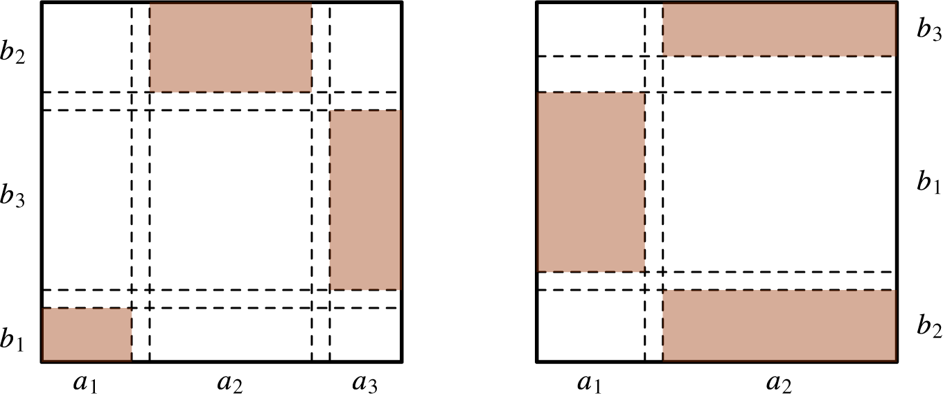
Figure 1 Defining maps for a Barański carpet with strictly positive dimension gap (left), and where the Assouad dimension of F is attained for correctly chosen parameters (right).
Proposition 4.1. For a Barański carpet F described above there is a strictly positive dimension gap, that is, there exists
 $\delta _F>0$
such that
$\delta _F>0$
such that
 $$ \begin{align*} \inf_{\mathbf{p}} \dim_{\mathrm{A}}\nu_{\mathbf{p}} \geqslant \dim_{\mathrm{A}}F + \delta_F. \end{align*} $$
Proof. The condition that there is no exact overlap when projecting to either coordinate axis implies that
 $p_1^{\sigma }(i)=p(i)$
and so
$p_1^{\sigma }(i)=p(i)$
and so
 $P_1^{\sigma }(i)=1$
for all
$P_1^{\sigma }(i)=1$
for all
 $i\in \mathcal {I}=\{1,\ldots ,N\}$
. Applying Theorem 2.5, we immediately obtain
$i\in \mathcal {I}=\{1,\ldots ,N\}$
. Applying Theorem 2.5, we immediately obtain
 $$ \begin{align*} \dim_{\mathrm{A}}\nu_{\mathbf{p}} = \max\bigg\{ \frac{\log p(i)}{\log a_i}, \frac{\log p(i)}{\log b_i}: i\in\mathcal{I} \bigg\}. \end{align*} $$
Since F is not in the Lalley–Gatzouras class and
 $s\geqslant t$
, there exists
$s\geqslant t$
, there exists
 $\ell \in \mathcal {I}$
such that
$\ell \in \mathcal {I}$
such that
 $b_{\ell }^s>a_{\ell }^s$
. Fix
$b_{\ell }^s>a_{\ell }^s$
. Fix
 $0<\varepsilon <b_{\ell }^s-a_{\ell }^s$
and first consider any
$0<\varepsilon <b_{\ell }^s-a_{\ell }^s$
and first consider any
 $\mathbf {p}$
that satisfies
$\mathbf {p}$
that satisfies
 $p(i)\leqslant a_i^s+\varepsilon $
for every
$p(i)\leqslant a_i^s+\varepsilon $
for every
 $i\in \mathcal {I}$
. Then
$i\in \mathcal {I}$
. Then
 $$ \begin{align*} \dim_{\mathrm{A}}\nu_{\mathbf{p}} \geqslant \frac{\log p(\ell)}{\log b_{\ell}} \geqslant \frac{\log (a_{\ell}^s+\varepsilon)}{\log b_{\ell}}> s \end{align*} $$
by the choice of
 $\varepsilon $
.
$\varepsilon $
.
Now assume that
 $\mathbf {p}$
is such that there exists
$\mathbf {p}$
is such that there exists
 $j\in \mathcal {I}$
satisfying
$j\in \mathcal {I}$
satisfying
 $p(j)>a_j^s+\varepsilon $
. Since
$p(j)>a_j^s+\varepsilon $
. Since
 $\sum _{i\in \mathcal {I}} a_i^s=1$
, the pigeonhole principle implies that there exists
$\sum _{i\in \mathcal {I}} a_i^s=1$
, the pigeonhole principle implies that there exists
 $k\in \mathcal {I}$
such that
$k\in \mathcal {I}$
such that
 $0<p(k)\leqslant a_k^s-\varepsilon /(N-1)$
. Using this particular index,
$0<p(k)\leqslant a_k^s-\varepsilon /(N-1)$
. Using this particular index,
 $$ \begin{align*} \dim_{\mathrm{A}}\nu_{\mathbf{p}} \geqslant \frac{\log p(k)}{\log a_{k}} \geqslant \frac{\log( a_k^s -\varepsilon/(N-1))}{\log a_k} = s+ \frac{\log( (1- \varepsilon\cdot a_k^{-s}/(N-1) ))}{\log a_k}> s. \end{align*} $$
Therefore, choosing
 $$ \begin{align*} \delta_F := \min \bigg\{ \frac{\log (a_{\ell}^s+\varepsilon)}{\log b_{\ell}} - s, \frac{\log( (1-\varepsilon\cdot a_k^{-s}/(N-1)))}{\log a_k} \bigg\} \end{align*} $$
completes the proof.
Proposition 4.1 shows that if a genuine Barański carpet whose Assouad dimension is realized by a self-affine measure exists, then its defining IFS must have at least three maps. Our second example shows that such a carpet does exist using only three maps. Giving a complete characterization for Barański carpets with three maps seems possible but perhaps tedious. However, it is straightforward to give an easy-to-check sufficient condition (valid for all Barański carpets) ensuring that the Assouad dimension of the carpet is attained by a Bernoulli measure. Comparing the formula from [Reference Fraser10] with Theorem 2.5 shows that
 $\dim _{\mathrm {A}}F = \max _{\sigma \in \mathcal {A}}\overline {S}(\mathbf {q}^{\sigma } ,\sigma )$
. Therefore, if
$\dim _{\mathrm {A}}F = \max _{\sigma \in \mathcal {A}}\overline {S}(\mathbf {q}^{\sigma } ,\sigma )$
. Therefore, if
 $\sigma $
satisfies
$\sigma $
satisfies
 $\overline {S}(\mathbf {q}^{\sigma } ,\sigma )\geqslant \max \{ \overline {S}(\mathbf {q}^{\omega } ,\omega ),\, \overline {S}(\mathbf {q}^{\sigma } ,\omega ) \}$
, then
$\overline {S}(\mathbf {q}^{\sigma } ,\sigma )\geqslant \max \{ \overline {S}(\mathbf {q}^{\omega } ,\omega ),\, \overline {S}(\mathbf {q}^{\sigma } ,\omega ) \}$
, then
 $\dim _{\mathrm {A}}F = \dim _{\mathrm {A}} \nu _{\mathbf {q}^{\sigma }}$
.
$\dim _{\mathrm {A}}F = \dim _{\mathrm {A}} \nu _{\mathbf {q}^{\sigma }}$
.
To demonstrate this, consider the Barański carpet whose first-level cylinders are depicted with the three shaded rectangles on the right-hand side of Figure 1. To ensure the attractor is a genuine Barański carpet, assume
 $a_1<b_1$
and
$a_1<b_1$
and
 $a_2> \min \{b_2,b_3\}$
. Define
$a_2> \min \{b_2,b_3\}$
. Define
 $r,s,t$
as follows:
$r,s,t$
as follows:
 $b_2^r+b_3^r=1,\, a_1^s+a_2^s=1$
and
$b_2^r+b_3^r=1,\, a_1^s+a_2^s=1$
and
 $b_1^t+b_2^t+b_3^t=1$
. We assume
$b_1^t+b_2^t+b_3^t=1$
. We assume
 $\max \{s,t\}<1$
so that the maps can be arranged in a way that satisfies the very strong SPPC. It follows from the formulas in [Reference Fraser10] that
$\max \{s,t\}<1$
so that the maps can be arranged in a way that satisfies the very strong SPPC. It follows from the formulas in [Reference Fraser10] that
 $\dim _{\mathrm {A}}F = \max \{s+r,t\}$
.
$\dim _{\mathrm {A}}F = \max \{s+r,t\}$
.
Proposition 4.2. Consider a Barański carpet as on the right-hand side of Figure 1. Assume
 $s+r> t$
. If
$s+r> t$
. If
 $a_2\geqslant \max \{b_2,b_3\}$
and
$a_2\geqslant \max \{b_2,b_3\}$
and
 $b_1^{1+r/s}\leqslant a_1<b_1$
, then
$b_1^{1+r/s}\leqslant a_1<b_1$
, then
 $\dim _{\mathrm {A}} F= \dim _{\mathrm {A}} \nu _{\mathbf {q}^{\sigma }}$
for
$\dim _{\mathrm {A}} F= \dim _{\mathrm {A}} \nu _{\mathbf {q}^{\sigma }}$
for
 $\sigma =(1,2)$
.
$\sigma =(1,2)$
.
Proof. Let
 $\sigma =(1,2)$
and
$\sigma =(1,2)$
and
 $\omega =(2,1)$
. The vector
$\omega =(2,1)$
. The vector
 $\mathbf {q}^{\sigma }$
is
$\mathbf {q}^{\sigma }$
is
 $$ \begin{align*} q(1)=a_1^s,\quad q(2) = a_2^s\cdot b_2^r,\quad q(3) = a_2^s\cdot b_3^r. \end{align*} $$
A simple calculation gives
 $\overline {S}(\mathbf {q}^{\sigma } ,\sigma )=s+r=\dim _{\mathrm {A}} F$
, because we assume
$\overline {S}(\mathbf {q}^{\sigma } ,\sigma )=s+r=\dim _{\mathrm {A}} F$
, because we assume
 $s+r>t$
. Hence, it is enough to check when
$s+r>t$
. Hence, it is enough to check when
 $\overline {S}(\mathbf {q}^{\sigma }, \omega )\leqslant s+r$
. Another calculation yields
$\overline {S}(\mathbf {q}^{\sigma }, \omega )\leqslant s+r$
. Another calculation yields
 $$ \begin{align*} \overline{S}(\mathbf{q}^{\sigma}, \omega) &= \max_{i\in\mathcal{I}_1^{\omega}} \frac{ \log P_{0}^{\omega}(i) }{ \log \unicode{x3bb}_{i}^{(\omega_1)} } + \max_{i\in\mathcal{I}_2^{\omega}} \frac{ \log P_{1}^{\omega}(i) }{ \log \unicode{x3bb}_{i}^{(\omega_2)} } \\ &= \max\bigg\{ s\cdot\frac{\log a_1}{\log b_1}, s\cdot\frac{\log a_2}{\log b_2} +r, s \cdot\frac{\log a_2}{\log b_3} +r \bigg\} + 0. \end{align*} $$
The last two terms are at most
 $s+r$
if and only if
$s+r$
if and only if
 $a_2\geqslant \max \{b_2,b_3\}$
and the first term is at most
$a_2\geqslant \max \{b_2,b_3\}$
and the first term is at most
 $s+r$
if and only if
$s+r$
if and only if
 $b_1^{1+r/s}\leqslant a_1$
, completing the proof.
$b_1^{1+r/s}\leqslant a_1$
, completing the proof.
4.2 Characterization of SPPC in dimension
 $3$
$3$

Recall from Lemma 3.2 that
 $\mathcal {A}=\mathcal {B}$
in
$\mathcal {A}=\mathcal {B}$
in
 $d=3$
and the notation
$d=3$
and the notation
 $y\prec x$
from (3.1). If no coordinate dominates any other, then (recall) F is a genuine Barański sponge and projection to any of the three principal planes is a Barański carpet. For genuine Barański sponges with
$y\prec x$
from (3.1). If no coordinate dominates any other, then (recall) F is a genuine Barański sponge and projection to any of the three principal planes is a Barański carpet. For genuine Barański sponges with
 $d=3$
, it is not necessarily true that
$d=3$
, it is not necessarily true that
 $\mathcal {B}=\mathcal {S}_3$
. For example, take an IFS consisting of two maps with
$\mathcal {B}=\mathcal {S}_3$
. For example, take an IFS consisting of two maps with
 $\unicode{x3bb} _1^{(3)}<\unicode{x3bb} _1^{(2)}<\unicode{x3bb} _1^{(1)}$
and
$\unicode{x3bb} _1^{(3)}<\unicode{x3bb} _1^{(2)}<\unicode{x3bb} _1^{(1)}$
and
 $\unicode{x3bb} _2^{(1)}<\unicode{x3bb} _2^{(2)}<\unicode{x3bb} _2^{(3)}$
. Depending on these parameters, only one of the orderings
$\unicode{x3bb} _2^{(1)}<\unicode{x3bb} _2^{(2)}<\unicode{x3bb} _2^{(3)}$
. Depending on these parameters, only one of the orderings
 $(1,3,2)$
and
$(1,3,2)$
and
 $(2,3,1)$
is an element of
$(2,3,1)$
is an element of
 $\mathcal {B}$
because there is no
$\mathcal {B}$
because there is no
 $\mathbf {p}\in \mathcal {P}_{\mathcal {I}}$
that simultaneously satisfies
$\mathbf {p}\in \mathcal {P}_{\mathcal {I}}$
that simultaneously satisfies
 $\chi _{1}(\mathbf {p}) < \chi _{3}(\mathbf {p}) < \chi _{2}(\mathbf {p})$
and
$\chi _{1}(\mathbf {p}) < \chi _{3}(\mathbf {p}) < \chi _{2}(\mathbf {p})$
and
 $\chi _{2}(\mathbf {p}) < \chi _{3}(\mathbf {p}) < \chi _{1}(\mathbf {p})$
. BY analogous reasoning, either
$\chi _{2}(\mathbf {p}) < \chi _{3}(\mathbf {p}) < \chi _{1}(\mathbf {p})$
. BY analogous reasoning, either
 $(2,1,3)\in \mathcal {B}$
or
$(2,1,3)\in \mathcal {B}$
or
 $(3,1,2)\in \mathcal {B}$
.
$(3,1,2)\in \mathcal {B}$
.
Assuming that
 $y\prec x$
, we have
$y\prec x$
, we have
 $\mathcal {A}\subseteq \{(x,y,z), (x,z,y), (z,x,y)\}$
. Hence, projection onto the
$\mathcal {A}\subseteq \{(x,y,z), (x,z,y), (z,x,y)\}$
. Hence, projection onto the
 $(y,z)$
-plane never plays a role. If
$(y,z)$
-plane never plays a role. If
 $\#\mathcal {A}=1$
, then F is a Lalley–Gatzouras sponge. There are potentially three possibilities for
$\#\mathcal {A}=1$
, then F is a Lalley–Gatzouras sponge. There are potentially three possibilities for
 $\#\mathcal {A}=2$
:
$\#\mathcal {A}=2$
:
-
(1)
$\mathcal {A}=\{(x,y,z),(x,z,y)\}$
, that is,
$\max \{y,z\}\prec x$
. In this case, the projections onto both the
$(x,y)$
- and
$(x,z)$
-planes are Lalley–Gatzouras carpets with x being the dominant side. -
(2)
$\mathcal {A}=\{(x,z,y),(z,x,y)\}$
, that is,
$y\prec \min \{x,z\}$
. In this case, projection onto the
$(x,z)$
-plane is a Barański carpet and
$y\prec \min \{x,z\}$
implies that projection onto either the
$(x,y)$
- or
$(y,z)$
-plane can be arbitrary.


The third option is not possible due to the following proposition.
Proposition 4.3. Let F be a three-dimensional sponge that satisfies the SPPC,
 $y\prec x$
and
$y\prec x$
and
 $(x,y,z),(z,x,y)\in \mathcal {A}$
. Then also
$(x,y,z),(z,x,y)\in \mathcal {A}$
. Then also
 $(x,z,y)\in \mathcal {A}$
.
$(x,z,y)\in \mathcal {A}$
.
Proof. All maps of the IFS defining F cannot be ordered the same way; therefore, without loss of generality we assume that
 $$ \begin{align} \unicode{x3bb}_1^{(z)} < \unicode{x3bb}_1^{(y)} < \unicode{x3bb}_1^{(x)} \quad\text{and}\quad \unicode{x3bb}_2^{(y)} < \unicode{x3bb}_2^{(x)} < \unicode{x3bb}_2^{(z)} \end{align} $$
corresponding to ordering
 $(x,y,z)$
and
$(x,y,z)$
and
 $(z,x,y)$
, respectively. We also assume that
$(z,x,y)$
, respectively. We also assume that
 $f_1$
and
$f_1$
and
 $f_2$
do not overlap exactly on either the
$f_2$
do not overlap exactly on either the
 $(x,y)$
- or
$(x,y)$
- or
 $(x,z)$
-plane.
$(x,z)$
-plane.
According to Lemma 3.1 it is enough to show that there exists
 $\mathbf {p}\in \mathcal {P}_{\mathcal {I}}$
such that
$\mathbf {p}\in \mathcal {P}_{\mathcal {I}}$
such that
 $\chi _x(\mathbf {p}) < \chi _{z}(\mathbf {p}) < \chi _{y}(\mathbf {p})$
. Consider
$\chi _x(\mathbf {p}) < \chi _{z}(\mathbf {p}) < \chi _{y}(\mathbf {p})$
. Consider
 $\mathbf {p}=(p,1-p,0,\ldots ,0)$
noting that the calculations that follow can also be adapted to small enough perturbations of
$\mathbf {p}=(p,1-p,0,\ldots ,0)$
noting that the calculations that follow can also be adapted to small enough perturbations of
 $\mathbf {p}$
. Straightforward algebraic manipulations yield
$\mathbf {p}$
. Straightforward algebraic manipulations yield
 $$ \begin{align*} \chi_x(\mathbf{p}) < \chi_{z}(\mathbf{p})\ {\Longleftrightarrow}\ p>A \quad\text{and}\quad \chi_{z}(\mathbf{p}) < \chi_{y}(\mathbf{p})\ {\Longleftrightarrow}\ p<B, \end{align*} $$
where
 $$ \begin{align*} A:= \frac{\log (\unicode{x3bb}_2^{(x)}/\unicode{x3bb}_2^{(z)})}{\log ( (\unicode{x3bb}_2^{(x)}\unicode{x3bb}_1^{(z)}) / (\unicode{x3bb}_2^{(z)}\unicode{x3bb}_1^{(x)}) )} \quad\text{and}\quad B:= \frac{\log (\unicode{x3bb}_2^{(y)}/\unicode{x3bb}_2^{(z)})}{\log ( (\unicode{x3bb}_2^{(y)}\unicode{x3bb}_1^{(z)}) / (\unicode{x3bb}_2^{(z)}\unicode{x3bb}_1^{(y)}) )}. \end{align*} $$
Additional manipulations show
 $A<B$
if and only if
$A<B$
if and only if
 $$ \begin{align*} \frac{\log (\unicode{x3bb}_1^{(z)}/\unicode{x3bb}_1^{(y)})}{\log ( \unicode{x3bb}_2^{(y)} / \unicode{x3bb}_2^{(z)} )} < \frac{\log (\unicode{x3bb}_1^{(z)}/\unicode{x3bb}_1^{(x)})}{\log ( \unicode{x3bb}_2^{(x)} / \unicode{x3bb}_2^{(z)} )}, \end{align*} $$
which is always true because of (4.1). This completes the proof.
5 Symbolic arguments
In this section we work on the symbolic space
 $\Sigma = \mathcal {I}^{\mathbb {N}}$
of all one-sided infinite words
$\Sigma = \mathcal {I}^{\mathbb {N}}$
of all one-sided infinite words
 $\mathbf {i}=i_1,i_2,\ldots $
with the Bernoulli measure
$\mathbf {i}=i_1,i_2,\ldots $
with the Bernoulli measure
 $\mu _{\mathbf {p}}=\mathbf {p}^{\mathbb {N}}$
. Recall the notation from §2. Throughout the section a
$\mu _{\mathbf {p}}=\mathbf {p}^{\mathbb {N}}$
. Recall the notation from §2. Throughout the section a
 $\sigma $
-order always refers to a cube as defined in (2.4). We define symbolic cubes whose images under the natural projection (1.1) well-approximate Euclidean balls on the sponge F. Let
$\sigma $
-order always refers to a cube as defined in (2.4). We define symbolic cubes whose images under the natural projection (1.1) well-approximate Euclidean balls on the sponge F. Let
 $\Sigma _{r}^{\sigma }:= \{\mathbf {i}\in \Sigma : \mathbf {i} \text { is } \sigma \text {-ordered at scale } r\}$
. We define the
$\Sigma _{r}^{\sigma }:= \{\mathbf {i}\in \Sigma : \mathbf {i} \text { is } \sigma \text {-ordered at scale } r\}$
. We define the
 $\sigma $
-ordered symbolic r-approximate cube containing
$\sigma $
-ordered symbolic r-approximate cube containing
 $\mathbf {i}\in \Sigma _{r}^{\sigma }$
to be
$\mathbf {i}\in \Sigma _{r}^{\sigma }$
to be
 $$ \begin{align} B_{\mathbf{i}}(r):= \{\mathbf{j} \in \Sigma: |\Pi_{n}^{\sigma} \mathbf{j} \wedge \Pi_{n}^{\sigma} \mathbf{i}| \geqslant L_{\mathbf{i}}(r, \sigma_{n}) \text { for every } 1 \leqslant n \leqslant d\}, \end{align} $$
where
 $\mathbf {i}\wedge \mathbf {j}$
denotes the longest common prefix of
$\mathbf {i}\wedge \mathbf {j}$
denotes the longest common prefix of
 $\mathbf {i}$
and
$\mathbf {i}$
and
 $\mathbf {j}$
. This is the natural extension of the notion of approximate squares used extensively in the study of planar carpets. Due to (2.2), the image
$\mathbf {j}$
. This is the natural extension of the notion of approximate squares used extensively in the study of planar carpets. Due to (2.2), the image
 $\pi (B_{\mathbf {i}}(r))$
is contained within a hypercuboid of
$\pi (B_{\mathbf {i}}(r))$
is contained within a hypercuboid of
 $[0,1]^d$
aligned with the coordinate axes with side lengths at most r. Observe that if
$[0,1]^d$
aligned with the coordinate axes with side lengths at most r. Observe that if
 $\mathbf {i}\in \Sigma _{r}^{\sigma }$
, then for all
$\mathbf {i}\in \Sigma _{r}^{\sigma }$
, then for all
 $\mathbf {j}\in B_{\mathbf {i}}(r)$
also
$\mathbf {j}\in B_{\mathbf {i}}(r)$
also
 $\mathbf {j}\in \Sigma _{r}^{\sigma }$
. Thus, we identify the
$\mathbf {j}\in \Sigma _{r}^{\sigma }$
. Thus, we identify the
 $\sigma $
-ordering of
$\sigma $
-ordering of
 $B_{\mathbf {i}}(r)$
with the
$B_{\mathbf {i}}(r)$
with the
 $\sigma $
-ordering of
$\sigma $
-ordering of
 $\mathbf {i}$
at scale r. If
$\mathbf {i}$
at scale r. If
 $\mathbf {i}\in \Sigma _{r}^{\sigma }$
, then the surjectivity of the maps
$\mathbf {i}\in \Sigma _{r}^{\sigma }$
, then the surjectivity of the maps
 $\Pi _n^{\sigma }$
implies that
$\Pi _n^{\sigma }$
implies that
 $B_{\mathbf {i}}(r)$
can be identified with a sequence of symbols of length
$B_{\mathbf {i}}(r)$
can be identified with a sequence of symbols of length
 $L_{\mathbf {i}}(r,\sigma _1)$
of the form
$L_{\mathbf {i}}(r,\sigma _1)$
of the form

where we set
 $L_{\mathbf {i}}(r,\sigma _{d+1}):= 0$
.
$L_{\mathbf {i}}(r,\sigma _{d+1}):= 0$
.
The following lemmas collect important properties about the
 $\mu _{\mathbf {p}}$
measure of a symbolic r-approximate cube. The first is the extension of [Reference Olsen21, equation (6.2)]. We use the convention that any empty product is equal to
$\mu _{\mathbf {p}}$
measure of a symbolic r-approximate cube. The first is the extension of [Reference Olsen21, equation (6.2)]. We use the convention that any empty product is equal to
 $1$
.
$1$
.
Lemma 5.1. The
 $\mu _{\mathbf {p}}$
measure of a
$\mu _{\mathbf {p}}$
measure of a
 $\sigma $
-ordered symbolic r-approximate cube is equal to
$\sigma $
-ordered symbolic r-approximate cube is equal to
 $$ \begin{align*} \mu_{\mathbf{p}}(B_{\mathbf{i}}(r)) = \prod_{n=1}^{d}\, \prod_{\ell=L_{\mathbf{i}}(r,\sigma_{n+1})+1}^{L_{\mathbf{i}}(r,\sigma_n)} p_n^{\sigma}(\Pi_n^{\sigma}i_{\ell}) = \prod_{n=1}^{d} \prod_{\ell=1}^{L_{\mathbf{i}}(r,\sigma_n)} P_{n-1}^{\sigma}(\Pi_{n}^{\sigma} i_{\ell}). \end{align*} $$
Proof. From definition (5.1) of
 $B_{\mathbf {i}}(r)$
it follows that an approximate cube is the disjoint union of level-
$B_{\mathbf {i}}(r)$
it follows that an approximate cube is the disjoint union of level-
 $L_{\mathbf {i}}(r,\sigma _1)$
cylinder sets:
$L_{\mathbf {i}}(r,\sigma _1)$
cylinder sets:
 $$ \begin{align*} \{ [j_1,\ldots,j_{L_{\mathbf{i}}(r,\sigma_1)}]: \Pi_{n}^{\sigma} j_{\ell}&=\Pi_n^{\sigma} i_{\ell} \text{ for } \ell=L_{\mathbf{i}}(r,\sigma_{n+1})\\&\quad+1,\ldots,L_{\mathbf{i}}(r,\sigma_n) \text{ and } 1\leqslant n\leqslant d \}. \end{align*} $$
For each such cylinder,
 $\mu _{\mathbf {p}}([j_1,\ldots ,j_{L_{\mathbf {i}}(r,\sigma _1)}]) = \prod _{\ell =1}^{L_{\mathbf {i}}(r,\sigma _1)} p(j_{\ell })$
. Summing and using multiplicativity, we obtain
$\mu _{\mathbf {p}}([j_1,\ldots ,j_{L_{\mathbf {i}}(r,\sigma _1)}]) = \prod _{\ell =1}^{L_{\mathbf {i}}(r,\sigma _1)} p(j_{\ell })$
. Summing and using multiplicativity, we obtain
 $$ \begin{align*} \mu_{\mathbf{p}}(B_{\mathbf{i}}(r)) = \prod_{n=1}^{d}\, \prod_{\ell=L_{\mathbf{i}}(r,\sigma_{n+1})+1}^{L_{\mathbf{i}}(r,\sigma_n)}\, \sum_{j\in\mathcal{I}: \Pi_n^{\sigma} j=\Pi_n^{\sigma} i_{\ell}} p(j) = \prod_{n=1}^{d}\, \prod_{\ell=L_{\mathbf{i}}(r,\sigma_{n+1})+1}^{L_{\mathbf{i}}(r,\sigma_n)}\, p_n^{\sigma}(\Pi_n^{\sigma} i_{\ell}). \end{align*} $$
The last equality in the assertion follows from definition (2.10) of
 $P_{n-1}^{\sigma }(\Pi _{n}^{\sigma } i_{\ell })$
.
$P_{n-1}^{\sigma }(\Pi _{n}^{\sigma } i_{\ell })$
.
Remark 5.2. Assume
 $B_{\mathbf {i}}(r)$
is
$B_{\mathbf {i}}(r)$
is
 $\sigma $
-ordered and
$\sigma $
-ordered and
 $L_{\mathbf {i}}(r,\sigma _m)=L_{\mathbf {i}}(r,\sigma _{m-1})=\cdots =L_{\mathbf {i}}(r,\sigma _{m-k})$
for some
$L_{\mathbf {i}}(r,\sigma _m)=L_{\mathbf {i}}(r,\sigma _{m-1})=\cdots =L_{\mathbf {i}}(r,\sigma _{m-k})$
for some
 $1\leqslant k< m\leqslant d$
. Then the formula for
$1\leqslant k< m\leqslant d$
. Then the formula for
 $\mu _{\mathbf {p}}(B_{\mathbf {i}}(r))$
can also be calculated using the ordering
$\mu _{\mathbf {p}}(B_{\mathbf {i}}(r))$
can also be calculated using the ordering
 $(\sigma _1,\ldots ,\sigma _{m-k-1},\omega ,\sigma _{m+1},\ldots ,\sigma _d)$
, where the first block is empty if
$(\sigma _1,\ldots ,\sigma _{m-k-1},\omega ,\sigma _{m+1},\ldots ,\sigma _d)$
, where the first block is empty if
 $k=m-1$
, the last block is empty if
$k=m-1$
, the last block is empty if
 $m=d$
and
$m=d$
and
 $\omega $
is any permutation of
$\omega $
is any permutation of
 $\sigma _m,\sigma _{m-1},\ldots ,\sigma _{m-k}$
.
$\sigma _m,\sigma _{m-1},\ldots ,\sigma _{m-k}$
.
Motivated by the definition of
 $\dim _{\mathrm {A}}\nu $
, the goal is to bound the ratio
$\dim _{\mathrm {A}}\nu $
, the goal is to bound the ratio
 $\mu _{\mathbf {p}}(B_{\mathbf {i}}(R))/\mu _{\mathbf {p}}(B_{\mathbf {i}}(r))$
for approximate cubes with different orderings. The first step is to consider when
$\mu _{\mathbf {p}}(B_{\mathbf {i}}(R))/\mu _{\mathbf {p}}(B_{\mathbf {i}}(r))$
for approximate cubes with different orderings. The first step is to consider when
 $B_{\mathbf {i}}(R)$
and
$B_{\mathbf {i}}(R)$
and
 $B_{\mathbf {i}}(r)$
have the same ordering.
$B_{\mathbf {i}}(r)$
have the same ordering.
Let
 $\unicode{x3bb} _{\min }:= \min _{n,i} \unicode{x3bb} _i^{(n)}$
and fix
$\unicode{x3bb} _{\min }:= \min _{n,i} \unicode{x3bb} _i^{(n)}$
and fix
 $\sigma \in \mathcal {A}$
. For
$\sigma \in \mathcal {A}$
. For
 $1\leqslant n\leqslant d$
, we introduce
$1\leqslant n\leqslant d$
, we introduce
 $$ \begin{align} \overline{k}_n^{\sigma} := \operatorname*{\mbox{arg max}}_{i\in\mathcal{I}_n^{\sigma}} \frac{ \log P_{n-1}^{\sigma}(i) }{ \log \unicode{x3bb}_{i}^{(\sigma_n)} },\quad \underline{k}_n^{\sigma} := \operatorname*{\mbox{arg min}}_{i\in\mathcal{I}_n^{\sigma}} \frac{ \log P_{n-1}^{\sigma}(i) }{ \log \unicode{x3bb}_{i}^{(\sigma_n)} } \end{align} $$
and
 $$ \begin{align} \overline{s}_n^{\sigma} := \frac{ \log P_{n-1}^{\sigma}(\overline{k}_n^{\sigma}) }{ \log \unicode{x3bb}_{\overline{k}_n^{\sigma}}^{(\sigma_n)} },\quad \underline{s}_n^{\sigma} := \frac{ \log P^\sigma_{n-1}(\underline{k}_n^{\sigma}) }{ \log \unicode{x3bb}_{\underline{k}_n^{\sigma}}^{(\sigma_n)} }. \end{align} $$
With this notation
 $\overline {S}(\mathbf {p},\sigma ) = \sum _{n=1}^d \overline {s}_n^{\sigma }$
and
$\overline {S}(\mathbf {p},\sigma ) = \sum _{n=1}^d \overline {s}_n^{\sigma }$
and
 $\underline {S}(\mathbf {p},\sigma ) = \sum _{n=1}^d \underline {s}_n^{\sigma }$
. If there are multiple choices for either
$\underline {S}(\mathbf {p},\sigma ) = \sum _{n=1}^d \underline {s}_n^{\sigma }$
. If there are multiple choices for either
 $\overline {k}_n^{\sigma }$
or
$\overline {k}_n^{\sigma }$
or
 $\underline {k}_n^{\sigma }$
, then choose one arbitrarily.
$\underline {k}_n^{\sigma }$
, then choose one arbitrarily.
Lemma 5.3. Fix
 $\sigma \in \mathcal {A}$
and assume that both
$\sigma \in \mathcal {A}$
and assume that both
 $B_{\mathbf {i}}(R)$
and
$B_{\mathbf {i}}(R)$
and
 $B_{\mathbf {i}}(r)$
are
$B_{\mathbf {i}}(r)$
are
 $\sigma $
-ordered, where
$\sigma $
-ordered, where
 $0<R\leqslant 1$
and
$0<R\leqslant 1$
and
 $r<\unicode{x3bb} _{\min } R$
. Then there exists a constant
$r<\unicode{x3bb} _{\min } R$
. Then there exists a constant
 $C>1$
depending only on the sponge F such that
$C>1$
depending only on the sponge F such that
 $$ \begin{align*} C^{-1} \bigg( \frac{R}{r} \bigg)^{ \underline{S}(\mathbf{p},\sigma) } \leqslant \frac{\mu_{\mathbf{p}}(B_{\mathbf{i}}(R))}{\mu_{\mathbf{p}}(B_{\mathbf{i}}(r))} \leqslant C \bigg( \frac{R}{r} \bigg)^{ \overline{S}(\mathbf{p},\sigma) }. \end{align*} $$
Proof. It follows from Lemma 5.1 that
 $$ \begin{align*} \frac{\mu_{\mathbf{p}}(B_{\mathbf{i}}(R))}{\mu_{\mathbf{p}}(B_{\mathbf{i}}(r))} &= \prod_{n=1}^{d}\, \prod_{\ell=L_{\mathbf{i}}(R,\sigma_n)+1}^{L_{\mathbf{i}}(r,\sigma_n)} \frac{1}{P_{n-1}^{\sigma}(\Pi_{n}^{\sigma}i_{\ell})}\\ &= \prod_{n=1}^{d}\, \prod_{\ell=L_{\mathbf{i}}(R,\sigma_n)+1}^{L_{\mathbf{i}}(r,\sigma_n)} ( \unicode{x3bb}_{\Pi_n^\sigma i_{\ell}}^{(\sigma_n)} )^{{\log P_{n-1}^{\sigma}(\Pi_{n}^{\sigma}i_{\ell})}/{-\!\log \unicode{x3bb}_{\Pi_n^{\sigma} i_{\ell}}^{(\sigma_n)} }}. \end{align*} $$
The requirement that
 $r<\unicode{x3bb} _{\min } R$
ensures that
$r<\unicode{x3bb} _{\min } R$
ensures that
 $L_{\mathbf {i}}(R,\sigma _n)<L_{\mathbf {i}}(r,\sigma _n)$
for all n. We bound each exponent individually to obtain
$L_{\mathbf {i}}(R,\sigma _n)<L_{\mathbf {i}}(r,\sigma _n)$
for all n. We bound each exponent individually to obtain
 $$ \begin{align} \prod_{n=1}^{d} \bigg( \prod_{\ell=L_{\mathbf{i}}(R,\sigma_n)+1}^{L_{\mathbf{i}}(r,\sigma_n)} \unicode{x3bb}_{\Pi_n^{\sigma} i_{\ell}}^{(\sigma_n)} \bigg)^{ -\underline{s}_n^{\sigma} } \leqslant \frac{\mu_{\mathbf{p}}(B_{\mathbf{i}}(R))}{\mu_{\mathbf{p}}(B_{\mathbf{i}}(r))} \leqslant \prod_{n=1}^{d} \bigg( \prod_{\ell=L_{\mathbf{i}}(R,\sigma_n)+1}^{L_{\mathbf{i}}(r,\sigma_n)} \unicode{x3bb}_{\Pi_n^{\sigma} i_{\ell}}^{(\sigma_n)} \bigg)^{ -\overline{s}_n^{\sigma} }. \end{align} $$
From definition (2.2) of
 $L_{\mathbf {i}}(r,n)$
it follows that there exists
$L_{\mathbf {i}}(r,n)$
it follows that there exists
 $C>1$
such that
$C>1$
such that
 $$ \begin{align} C^{-1} \cdot\frac{r}{R}\leqslant \prod_{\ell=L_{\mathbf{i}}(R,n)+1}^{L_{\mathbf{i}}(r,n)} \unicode{x3bb}_{i_{\ell}}^{(n)} \leqslant C\cdot \frac{r}{R}, \end{align} $$
which together with (5.4) concludes the proof.
Now we extend Lemma 5.3 so that
 $B_{\mathbf {i}}(R)$
and
$B_{\mathbf {i}}(R)$
and
 $B_{\mathbf {i}}(r)$
can have different orderings. This step, which represents one of the key technical challenges in the paper, is not necessary if F is a Lalley–Gatzouras sponge.
$B_{\mathbf {i}}(r)$
can have different orderings. This step, which represents one of the key technical challenges in the paper, is not necessary if F is a Lalley–Gatzouras sponge.
Proposition 5.4. Assume
 $0<R\leqslant 1$
and
$0<R\leqslant 1$
and
 $r<\unicode{x3bb} _{\min } R$
. Then there exists a constant
$r<\unicode{x3bb} _{\min } R$
. Then there exists a constant
 $C>1$
depending only on the sponge F such that
$C>1$
depending only on the sponge F such that
 $$ \begin{align*} C^{-1} \bigg( \frac{R}{r} \bigg)^{ \min_{\sigma\in\mathcal{A}} \underline{S}(\mathbf{p},\sigma) } \leqslant \frac{\mu_{\mathbf{p}}(B_{\mathbf{i}}(R))}{\mu_{\mathbf{p}}(B_{\mathbf{i}}(r))} \leqslant C \bigg( \frac{R}{r} \bigg)^{ \max_{\sigma\in\mathcal{A}} \overline{S}(\mathbf{p},\sigma) }. \end{align*} $$
5.1 Proof of Proposition 5.4
Let
 $\sigma _{\mathbf {i}}(r)$
denote the ordering of
$\sigma _{\mathbf {i}}(r)$
denote the ordering of
 $B_{\mathbf {i}}(r)$
and assume
$B_{\mathbf {i}}(r)$
and assume
 $\sigma _{\mathbf {i}}(R)\neq \sigma _{\mathbf {i}}(r)$
. Trying to estimate the ratio
$\sigma _{\mathbf {i}}(R)\neq \sigma _{\mathbf {i}}(r)$
. Trying to estimate the ratio
 $\mu _{\mathbf {p}}(B_{\mathbf {i}}(R))/\mu _{\mathbf {p}}(B_{\mathbf {i}}(r))$
directly using Lemma 5.1 did not lead us to a proof. Instead, the rough idea is to divide the interval
$\mu _{\mathbf {p}}(B_{\mathbf {i}}(R))/\mu _{\mathbf {p}}(B_{\mathbf {i}}(r))$
directly using Lemma 5.1 did not lead us to a proof. Instead, the rough idea is to divide the interval
 $[r,R]$
of scales into a uniformly bounded number of subintervals so that the ordering at roughly the two endpoints of a subinterval is the same. Then we repeatedly apply Lemma 5.3 to each subinterval. The next lemma allows us to make a subdivision.
$[r,R]$
of scales into a uniformly bounded number of subintervals so that the ordering at roughly the two endpoints of a subinterval is the same. Then we repeatedly apply Lemma 5.3 to each subinterval. The next lemma allows us to make a subdivision.
Lemma 5.5. Fix
 $\varepsilon>0$
such that
$\varepsilon>0$
such that
 $1-\varepsilon> \max _{n,i} \unicode{x3bb} _i^{(n)}$
. There exists a constant
$1-\varepsilon> \max _{n,i} \unicode{x3bb} _i^{(n)}$
. There exists a constant
 $C_1=C_1(F,\mathbf {p},\varepsilon )<\infty $
such that for all
$C_1=C_1(F,\mathbf {p},\varepsilon )<\infty $
such that for all
 $\mathbf {i}\in \Sigma $
and
$\mathbf {i}\in \Sigma $
and
 $0<R\leqslant 1$
,
$0<R\leqslant 1$
,
 $$ \begin{align*} \frac{\mu_{\mathbf{p}}(B_{\mathbf{i}}(R))}{\mu_{\mathbf{p}}(B_{\mathbf{i}}((1-\varepsilon)R))} \leqslant C_1. \end{align*} $$
Proof. First assume that
 $\sigma _{\mathbf {i}}(R)= \sigma _{\mathbf {i}}((1-\varepsilon )R)=\sigma $
and consider the symbolic representation of
$\sigma _{\mathbf {i}}(R)= \sigma _{\mathbf {i}}((1-\varepsilon )R)=\sigma $
and consider the symbolic representation of
 $B_{\mathbf {i}}(R)$
and
$B_{\mathbf {i}}(R)$
and
 $B_{\mathbf {i}}((1-\varepsilon )R)$
. They could be different at indices
$B_{\mathbf {i}}((1-\varepsilon )R)$
. They could be different at indices
 $$ \begin{align*} L_{\mathbf{i}}(R,\sigma_n)+1,\ldots, L_{\mathbf{i}}(R,\sigma_n)+ d-n+1 \quad\text{for each } 1\leqslant n\leqslant d, \end{align*} $$
but necessarily agree at all other indices due to the choice of
 $\varepsilon $
. Where they agree, the corresponding terms simply cancel out in
$\varepsilon $
. Where they agree, the corresponding terms simply cancel out in
 $\mu _{\mathbf {p}}(B_{\mathbf {i}}(R)) / \mu _{\mathbf {p}}(B_{\mathbf {i}}((1-\varepsilon )R))$
. Hence, there are at most
$\mu _{\mathbf {p}}(B_{\mathbf {i}}(R)) / \mu _{\mathbf {p}}(B_{\mathbf {i}}((1-\varepsilon )R))$
. Hence, there are at most
 $1+2+\cdots +d<d^2$
different indices of interest. An index where they differ corresponds in
$1+2+\cdots +d<d^2$
different indices of interest. An index where they differ corresponds in
 $\mu _{\mathbf {p}}(B_{\mathbf {i}}(R)) / \mu _{\mathbf {p}}(B_{\mathbf {i}}((1-\varepsilon )R))$
to a ratio
$\mu _{\mathbf {p}}(B_{\mathbf {i}}(R)) / \mu _{\mathbf {p}}(B_{\mathbf {i}}((1-\varepsilon )R))$
to a ratio
 $p/q$
, where
$p/q$
, where
 $p\geqslant q$
(p is a sum containing q by (2.9)) and both
$p\geqslant q$
(p is a sum containing q by (2.9)) and both
 $p,q$
are uniformly bounded away from
$p,q$
are uniformly bounded away from
 $0$
(simply because p and q are sums of different terms of
$0$
(simply because p and q are sums of different terms of
 $\mathbf {p}$
which all are strictly positive to begin with). Therefore, there exists a uniform upper bound C for
$\mathbf {p}$
which all are strictly positive to begin with). Therefore, there exists a uniform upper bound C for
 $p/q$
. As a result,
$p/q$
. As a result,
 $$ \begin{align*} \frac{\mu_{\mathbf{p}}(B_{\mathbf{i}}(R))}{\mu_{\mathbf{p}}(B_{\mathbf{i}}((1-\varepsilon)R))} \leqslant C^{d^2}, \end{align*} $$
completing the proof in this case by setting
 $C_1=C^{d^2}$
.
$C_1=C^{d^2}$
.
We claim that even if
 $\sigma _{\mathbf {i}}(R)\neq \sigma _{\mathbf {i}}((1-\varepsilon )R)$
, there still exists an ordering
$\sigma _{\mathbf {i}}(R)\neq \sigma _{\mathbf {i}}((1-\varepsilon )R)$
, there still exists an ordering
 $\omega $
such that the value of
$\omega $
such that the value of
 $\mu _{\mathbf {p}}(B_{\mathbf {i}}(R))$
is the same when calculating it with
$\mu _{\mathbf {p}}(B_{\mathbf {i}}(R))$
is the same when calculating it with
 $\sigma _{\mathbf {i}}(R)$
or
$\sigma _{\mathbf {i}}(R)$
or
 $\omega $
, and likewise the value of
$\omega $
, and likewise the value of
 $\mu _{\mathbf {p}}(B_{\mathbf {i}}((1-\varepsilon )R))$
is the same when calculating it with
$\mu _{\mathbf {p}}(B_{\mathbf {i}}((1-\varepsilon )R))$
is the same when calculating it with
 $\sigma _{\mathbf {i}}((1-\varepsilon )R)$
or
$\sigma _{\mathbf {i}}((1-\varepsilon )R)$
or
 $\omega $
. Hence, we may apply the previous argument to
$\omega $
. Hence, we may apply the previous argument to
 $\omega $
.
$\omega $
.
To see the claim, first observe that the ordering
 $\sigma _{\mathbf {i}}(R)=\sigma $
can be partitioned into
$\sigma _{\mathbf {i}}(R)=\sigma $
can be partitioned into
 $1\leqslant K\leqslant d$
blocks along indices
$1\leqslant K\leqslant d$
blocks along indices
 $d\geqslant n_1>n_2>\cdots >n_K=1$
so that
$d\geqslant n_1>n_2>\cdots >n_K=1$
so that
 $$ \begin{align*} L_{\mathbf{i}}(R,\sigma_d) = \cdots = L_{\mathbf{i}}(R,\sigma_{n_1}) < L_{\mathbf{i}}(R,&\sigma_{n_1+1}) = \cdots = L_{\mathbf{i}}(R,\sigma_{n_2}) \\ &\quad <\cdots< L_{\mathbf{i}}(R,\sigma_{n_{K-1}+1}) = \cdots = L_{\mathbf{i}}(R,\sigma_{n_K}). \end{align*} $$
The assumption on
 $\varepsilon $
implies that
$\varepsilon $
implies that
 $L_{\mathbf {i}}((1\kern-1pt -\varepsilon )R,n)-L_{\mathbf {i}}(R,n)\kern-1pt\in\kern-1pt \{0,\kern-1pt 1\}$
for all coordinates n. Therefore, we can partition the block
$L_{\mathbf {i}}((1\kern-1pt -\varepsilon )R,n)-L_{\mathbf {i}}(R,n)\kern-1pt\in\kern-1pt \{0,\kern-1pt 1\}$
for all coordinates n. Therefore, we can partition the block
 $X_{\ell }:= \{\sigma _{n_{\ell }},\ldots ,\sigma _{n_{\ell -1}+1}\}$
into
$X_{\ell }:= \{\sigma _{n_{\ell }},\ldots ,\sigma _{n_{\ell -1}+1}\}$
into
 $Y_{\ell }\sqcup Z_{\ell }$
, where
$Y_{\ell }\sqcup Z_{\ell }$
, where
 $Y_{\ell }=\{n\in X_{\ell }: L_{\mathbf {i}}((1-\varepsilon )R,n)=L_{\mathbf {i}}(R,n)\}$
and
$Y_{\ell }=\{n\in X_{\ell }: L_{\mathbf {i}}((1-\varepsilon )R,n)=L_{\mathbf {i}}(R,n)\}$
and
 $Z_{\ell }=\{n\in X_{\ell }: L_{\mathbf {i}}((1-\varepsilon )R,n)=L_{\mathbf {i}}(R,n)+1\}$
. We fix an (arbitrary) ordering of all
$Z_{\ell }=\{n\in X_{\ell }: L_{\mathbf {i}}((1-\varepsilon )R,n)=L_{\mathbf {i}}(R,n)+1\}$
. We fix an (arbitrary) ordering of all
 $Y_{\ell }$
,
$Y_{\ell }$
,
 $Z_{\ell }$
and define
$Z_{\ell }$
and define
 $$ \begin{align*} \omega:= (Z_K,Y_K,Z_{K-1},Y_{K-1},\ldots,Z_2,Y_2,Z_1,Y_1). \end{align*} $$
By Remark 5.2,
 $\mu _{\mathbf {p}}(B_{\mathbf {i}}(R))$
can be calculated by another ordering that only permutes elements within any of the blocks
$\mu _{\mathbf {p}}(B_{\mathbf {i}}(R))$
can be calculated by another ordering that only permutes elements within any of the blocks
 $X_{\ell }$
. The ordering
$X_{\ell }$
. The ordering
 $\omega $
clearly satisfies this. It remains to argue that
$\omega $
clearly satisfies this. It remains to argue that
 $\omega $
also works for
$\omega $
also works for
 $\sigma _{\mathbf {i}}((1-\varepsilon )R)$
.
$\sigma _{\mathbf {i}}((1-\varepsilon )R)$
.
If
 $n\in Y_{\ell }$
and
$n\in Y_{\ell }$
and
 $m\in Z_\ell $
(for some
$m\in Z_\ell $
(for some
 $1\leqslant \ell \leqslant K$
) then by definition
$1\leqslant \ell \leqslant K$
) then by definition
 $L_{\mathbf {i}}((1-\varepsilon )R,n) < L_{\mathbf {i}}((1-\varepsilon )R,m)$
. Moreover, If
$L_{\mathbf {i}}((1-\varepsilon )R,n) < L_{\mathbf {i}}((1-\varepsilon )R,m)$
. Moreover, If
 $n\in Z_{\ell }$
and
$n\in Z_{\ell }$
and
 $m\in Y_{\ell +1}$
(for some
$m\in Y_{\ell +1}$
(for some
 $1\leqslant \ell \leqslant K-1$
) then we also have
$1\leqslant \ell \leqslant K-1$
) then we also have
 $L_{\mathbf {i}}((1-\varepsilon )R,n) \leqslant L_{\mathbf {i}}((1-\varepsilon )R,m)$
. These imply that
$L_{\mathbf {i}}((1-\varepsilon )R,n) \leqslant L_{\mathbf {i}}((1-\varepsilon )R,m)$
. These imply that
 $\sigma _{\mathbf {i}}((1-\varepsilon )R)$
can be obtained from
$\sigma _{\mathbf {i}}((1-\varepsilon )R)$
can be obtained from
 $\omega $
by only permuting elements within a block
$\omega $
by only permuting elements within a block
 $Y_{\ell }$
or
$Y_{\ell }$
or
 $Z_{\ell }$
. This exactly means that
$Z_{\ell }$
. This exactly means that
 $\mu _{\mathbf {p}}(B_{\mathbf {i}}((1-\varepsilon )R))$
can be calculated using
$\mu _{\mathbf {p}}(B_{\mathbf {i}}((1-\varepsilon )R))$
can be calculated using
 $\omega $
.
$\omega $
.
We next define the scales where we subdivide
 $[r,R]$
. Let
$[r,R]$
. Let
 $$ \begin{align*} R_1:= \inf\{ r'>r: \sigma_{\mathbf{i}}(r')=\sigma_{\mathbf{i}}(R) \} \end{align*} $$
and terminate if
 $\sigma _{\mathbf {i}}((1-\varepsilon )R_{1})=\sigma _{\mathbf {i}}(r)$
, otherwise, for
$\sigma _{\mathbf {i}}((1-\varepsilon )R_{1})=\sigma _{\mathbf {i}}(r)$
, otherwise, for
 $k\geqslant 2$
until
$k\geqslant 2$
until
 $\sigma _{\mathbf {i}}((1-\varepsilon )R_{k})=\sigma _{\mathbf {i}}(r)$
define
$\sigma _{\mathbf {i}}((1-\varepsilon )R_{k})=\sigma _{\mathbf {i}}(r)$
define
 $$ \begin{align*} R_k:= \inf\{ r'>r: \sigma_{\mathbf{i}}(r') = \sigma_{\mathbf{i}}((1-\varepsilon)R_{k-1}) \} \end{align*} $$
concluding with
 $R_M$
, where
$R_M$
, where
 $\varepsilon =\varepsilon (r)>0$
is chosen so small that
$\varepsilon =\varepsilon (r)>0$
is chosen so small that
 $1-\varepsilon > \max \{r/R_M, \max _{n,i} \unicode{x3bb} _i^{(n)}\}$
. It follows from the construction that
$1-\varepsilon > \max \{r/R_M, \max _{n,i} \unicode{x3bb} _i^{(n)}\}$
. It follows from the construction that
 $\sigma _{\mathbf {i}}((1-\varepsilon )R_{k})$
is always different from the previous orderings, hence
$\sigma _{\mathbf {i}}((1-\varepsilon )R_{k})$
is always different from the previous orderings, hence
 $M\leqslant d!$
.
$M\leqslant d!$
.
We are ready to conclude the proof. We suppress multiplicative constants c depending only on F by writing
 $X\lesssim Y$
if
$X\lesssim Y$
if
 $X\leqslant cY$
. Using first Lemma 5.5 and then Lemma 5.3, we get the upper bound
$X\leqslant cY$
. Using first Lemma 5.5 and then Lemma 5.3, we get the upper bound
 $$ \begin{align*} \frac{\mu_{\mathbf{p}}(B_{\mathbf{i}}(R))}{\mu_{\mathbf{p}}(B_{\mathbf{i}}(r))} &\lesssim \frac{\mu_{\mathbf{p}}(B_{\mathbf{i}}(R))}{\mu_{\mathbf{p}}(B_{\mathbf{i}}(R_1))} \cdot \prod_{k=2}^M \frac{\mu_{\mathbf{p}}(B_{\mathbf{i}}((1-\varepsilon)R_{k-1}))}{\mu_{\mathbf{p}}(B_{\mathbf{i}}(R_k))} \cdot \frac{\mu_{\mathbf{p}}(B_{\mathbf{i}}((1-\varepsilon)R_M))}{\mu_{\mathbf{p}}(B_{\mathbf{i}}(r))} \\ &\lesssim \bigg( \frac{R}{R_1} \bigg)^{ \overline{S}(\mathbf{p},\sigma_{\mathbf{i}}(R_1)) } \prod_{k=2}^M \bigg( \frac{(1-\varepsilon)R_{k-1}}{R_k} \bigg)^{ \overline{S}(\mathbf{p},\sigma_{\mathbf{i}}(R_k)) } \bigg( \frac{(1-\varepsilon)R_M}{r} \bigg)^{ \overline{S}(\mathbf{p},\sigma_{\mathbf{i}}(r)) } \\ &\lesssim \bigg( \frac{R}{r} \bigg)^{ \max_{\sigma\in\mathcal{A}} \overline{S}(\mathbf{p},\sigma) }. \end{align*} $$
The lower bound is very similar. Lemma 5.5 is not necessary because
 $\mu _{\mathbf {p}}(B_{\mathbf {i}}(R)) \geqslant \mu _{\mathbf {p}}(B_{\mathbf {i}}((1-\varepsilon )R))$
holds for any
$\mu _{\mathbf {p}}(B_{\mathbf {i}}(R)) \geqslant \mu _{\mathbf {p}}(B_{\mathbf {i}}((1-\varepsilon )R))$
holds for any
 $R>0$
and one uses
$R>0$
and one uses
 $\min _{\sigma \in \mathcal {A}} \underline {S}(\mathbf {p},\sigma )$
instead in the last step. The proof of Proposition 5.4 is complete.
$\min _{\sigma \in \mathcal {A}} \underline {S}(\mathbf {p},\sigma )$
instead in the last step. The proof of Proposition 5.4 is complete.
6 Proof of Theorem 2.5
6.1 Transferring symbolic estimates to geometric estimates
The very strong SPPC implies that there exists
 $\delta _0>0$
depending only on the sponge F such that for every
$\delta _0>0$
depending only on the sponge F such that for every
 $\sigma \in \mathcal {A}$
,
$\sigma \in \mathcal {A}$
,
 $1\leqslant n\leqslant d$
and
$1\leqslant n\leqslant d$
and
 $i,j\in \mathcal {I}$
for which
$i,j\in \mathcal {I}$
for which
 $f_i$
and
$f_i$
and
 $f_j$
do not overlap exactly on
$f_j$
do not overlap exactly on
 $E_n^{\sigma }$
,
$E_n^{\sigma }$
,
 $$ \begin{align*} \mathrm{dist}( \Pi_n^{\sigma}(f_i([0,1]^d)), \Pi_n^{\sigma}(f_j([0,1]^d)) ) \geqslant \delta_0. \end{align*} $$
The next lemma allows us to replace a Euclidean ball
 $B(x,r)$
with the image of an approximate cube of roughly the same diameter under the natural projection
$B(x,r)$
with the image of an approximate cube of roughly the same diameter under the natural projection
 $\pi $
; recall (1.1). It is an adaptation of [Reference Olsen21, Proposition 6.2.1]. The short proof is included for completeness.
$\pi $
; recall (1.1). It is an adaptation of [Reference Olsen21, Proposition 6.2.1]. The short proof is included for completeness.
Lemma 6.1. Assume the sponge F satisfies the SPPC. For all
 $\mathbf {i}\in \Sigma $
and
$\mathbf {i}\in \Sigma $
and
 $r>0$
,
$r>0$
,
 $$ \begin{align*} \pi(B_{\mathbf{i}}(r)) \subseteq B(\pi(\mathbf{i}),\sqrt{d}\cdot r). \end{align*} $$
Moreover, if F satisfies the very strong SPPC, then
 $$ \begin{align*} B(\pi(\mathbf{i}), \delta_0 \cdot r)\cap F \subseteq \pi(B_{\mathbf{i}}(r)). \end{align*} $$
Proof. By definition (5.1), the image
 $\pi (B_{\mathbf {i}}(r))$
is contained inside a cuboid of side length
$\pi (B_{\mathbf {i}}(r))$
is contained inside a cuboid of side length
 $\prod _{\ell =1}^{L_{\mathbf {i}}(r,n)} \unicode{x3bb} _{i_\ell }^{(n)} \leqslant r$
in each coordinate n. In the worst case,
$\prod _{\ell =1}^{L_{\mathbf {i}}(r,n)} \unicode{x3bb} _{i_\ell }^{(n)} \leqslant r$
in each coordinate n. In the worst case,
 $\pi (\mathbf {i})$
is a corner of this cuboid which is then certainly contained in
$\pi (\mathbf {i})$
is a corner of this cuboid which is then certainly contained in
 $B(\pi (\mathbf {i}),\sqrt {d}\cdot r)$
.
$B(\pi (\mathbf {i}),\sqrt {d}\cdot r)$
.
We show that
 $\mathbf {j}\notin B_{\mathbf {i}}(r)$
implies
$\mathbf {j}\notin B_{\mathbf {i}}(r)$
implies
 $\pi (\mathbf {j})\notin B(\pi (\mathbf {i}), \delta _0 \cdot r)$
under the very strong SPPC. Assume
$\pi (\mathbf {j})\notin B(\pi (\mathbf {i}), \delta _0 \cdot r)$
under the very strong SPPC. Assume
 $B_{\mathbf {i}}(r)$
is
$B_{\mathbf {i}}(r)$
is
 $\sigma $
-ordered. Since
$\sigma $
-ordered. Since
 $\mathbf {j}\notin B_{\mathbf {i}}(r)$
, there exist a largest
$\mathbf {j}\notin B_{\mathbf {i}}(r)$
, there exist a largest
 $n'\in \{1,\ldots ,d\}$
and a smallest
$n'\in \{1,\ldots ,d\}$
and a smallest
 $\ell '\in \{L_{\mathbf {i}}(r,\sigma _{n'+1})+1,\ldots ,L_{\mathbf {i}}(r,\sigma _{n'})\}$
such that
$\ell '\in \{L_{\mathbf {i}}(r,\sigma _{n'+1})+1,\ldots ,L_{\mathbf {i}}(r,\sigma _{n'})\}$
such that
 $\Pi _{n'}^{\sigma }j_{\ell '}\neq \Pi _{n'}^{\sigma }i_{\ell '}$
. For this particular choice, the very strong SPPC implies that
$\Pi _{n'}^{\sigma }j_{\ell '}\neq \Pi _{n'}^{\sigma }i_{\ell '}$
. For this particular choice, the very strong SPPC implies that
 $$ \begin{align*} \mathrm{dist}( \Pi_{n'}^{\sigma}(f_{i_{\ell'}}([0,1]^d)), \Pi_{n'}^{\sigma}(f_{j_{\ell'}}([0,1]^d)) ) \geqslant \delta_0. \end{align*} $$
Since the projection
 $\Pi _{n'}^{\sigma }$
can only decrease distance and
$\Pi _{n'}^{\sigma }$
can only decrease distance and
 $\Pi _{n'}^{\sigma }j_{\ell }= \Pi _{n'}^{\sigma }i_{\ell }$
for all
$\Pi _{n'}^{\sigma }j_{\ell }= \Pi _{n'}^{\sigma }i_{\ell }$
for all
 $\ell <\ell '$
, we can bound
$\ell <\ell '$
, we can bound
 $$ \begin{align*} \mathrm{dist}(\pi(\mathbf{i}),\pi(\mathbf{j})) &\geqslant \mathrm{dist}(\Pi_{n'}^{\sigma}(\pi(\mathbf{i})),\Pi_{n'}^{\sigma}(\pi(\mathbf{j}))) \\ &\geqslant \mathrm{dist}(\Pi_{n'}^{\sigma}(f_{i_1\ldots i_{\ell'-1}i_{\ell'}}([0,1]^d)), \Pi_{n'}^{\sigma}(f_{j_1\ldots j_{\ell'-1}j_{\ell'}}([0,1]^d))) \\ &\geqslant \delta_0\cdot \prod_{\ell=1}^{\ell'-1} \unicode{x3bb}_{i_\ell}^{(\sigma_{n'})} \\ &\stackrel{(2.2)}{>} \delta_0\cdot r, \end{align*} $$
completing the proof.
The very strong SPPC also implies that the natural projection
 $\pi $
is injective and that
$\pi $
is injective and that
 $\mu _{\mathbf {p}}(B_{\mathbf {i}}(r))=\nu _{\mathbf {p}}(\pi (B_{\mathbf {i}}(r)))$
for any approximate cube
$\mu _{\mathbf {p}}(B_{\mathbf {i}}(r))=\nu _{\mathbf {p}}(\pi (B_{\mathbf {i}}(r)))$
for any approximate cube
 $B_{\mathbf {i}}(r)$
. This, together with Lemma 6.1, implies that for any
$B_{\mathbf {i}}(r)$
. This, together with Lemma 6.1, implies that for any
 $\mathbf {i}\in \Sigma $
and
$\mathbf {i}\in \Sigma $
and
 $0<r<R\leqslant 1$
,
$0<r<R\leqslant 1$
,
 $$ \begin{align*} \frac{\mu_{\mathbf{p}}(B_{\mathbf{i}}(R/\sqrt{d}))}{\mu_{\mathbf{p}}(B_{\mathbf{i}}(r/\delta_0))} \leqslant \frac{\nu_{\mathbf{p}}(B(\pi(\mathbf{i}),R))}{\nu_{\mathbf{p}}(B(\pi(\mathbf{i}),r))} \leqslant \frac{\mu_{\mathbf{p}}(B_{\mathbf{i}}(R/\delta_0))}{\mu_{\mathbf{p}}(B_{\mathbf{i}}(r/\sqrt{d}))}. \end{align*} $$
Hence, it is enough to consider the ratio
 $\mu _{\mathbf {p}}(B_{\mathbf {i}}(R))/\mu _{\mathbf {p}}(B_{\mathbf {i}}(r))$
.
$\mu _{\mathbf {p}}(B_{\mathbf {i}}(R))/\mu _{\mathbf {p}}(B_{\mathbf {i}}(r))$
.
The upper bound for
 $\dim _{\mathrm {A}}\nu _{\mathbf {p}}$
and the lower bound for
$\dim _{\mathrm {A}}\nu _{\mathbf {p}}$
and the lower bound for
 $\dim _{\mathrm {L}}\nu _{\mathbf {p}}$
now directly follow from Proposition 5.4. The lower bound for
$\dim _{\mathrm {L}}\nu _{\mathbf {p}}$
now directly follow from Proposition 5.4. The lower bound for
 $\dim _{\mathrm {A}}\nu _{\mathbf {p}}$
requires more work and we give the argument in the next subsection. The argument for the upper bound for
$\dim _{\mathrm {A}}\nu _{\mathbf {p}}$
requires more work and we give the argument in the next subsection. The argument for the upper bound for
 $\dim _{\mathrm {L}}\nu _{\mathbf {p}}$
is analogous and we omit the details.
$\dim _{\mathrm {L}}\nu _{\mathbf {p}}$
is analogous and we omit the details.
6.2 Lower bound for Assouad dimension
Recall the notation from (5.2) and (5.3). Using Lemma 6.1, in order to bound
 $\dim _{\mathrm {A}}\nu _{\mathbf {p}}$
from below, it suffices to prove the following proposition.
$\dim _{\mathrm {A}}\nu _{\mathbf {p}}$
from below, it suffices to prove the following proposition.
Proposition 6.2. For all
 $\sigma \in \mathcal {B}$
, there exists a sequence of triples
$\sigma \in \mathcal {B}$
, there exists a sequence of triples
 $(R, r, \mathbf {i}) \in (0,1) \times (0,1) \times \Sigma $
with
$(R, r, \mathbf {i}) \in (0,1) \times (0,1) \times \Sigma $
with
 $R/r\to \infty $
such that
$R/r\to \infty $
such that
 $$ \begin{align*} \frac{\mu_{\mathbf{p}}(B_{\mathbf{i}}(R))}{\mu_{\mathbf{p}}(B_{\mathbf{i}}(r))} \geqslant c \bigg( \frac{R}{r} \bigg)^{ \overline{S}(\mathbf{p},\sigma) } \end{align*} $$
for some constant
 $c>0$
uniformly for all triples in the sequence.
$c>0$
uniformly for all triples in the sequence.
Proof. Fix
 $\sigma \in \mathcal {B}$
. By definition of
$\sigma \in \mathcal {B}$
. By definition of
 $\mathcal {B}$
, there exist
$\mathcal {B}$
, there exist
 $\mathbf {j} \in \Sigma $
and
$\mathbf {j} \in \Sigma $
and
 $\rho>0$
such that
$\rho>0$
such that
 $\mathbf {j}$
determines a strictly
$\mathbf {j}$
determines a strictly
 $\sigma $
-ordered cylinder at scale
$\sigma $
-ordered cylinder at scale
 $\rho $
; see (2.3). By passing to a finite iterate of the original IFS if necessary, we may assume that
$\rho $
; see (2.3). By passing to a finite iterate of the original IFS if necessary, we may assume that
 $L_{\mathbf {j}}(\rho ,\sigma _d) = 1$
. Therefore, there exists
$L_{\mathbf {j}}(\rho ,\sigma _d) = 1$
. Therefore, there exists
 $j \in \mathcal {I}$
with
$j \in \mathcal {I}$
with
 $$ \begin{align*} \unicode{x3bb}_{j}^{(\sigma_d)} < \unicode{x3bb}_{j}^{(\sigma_{d-1})} < \cdots < \unicode{x3bb}_{j}^{(\sigma_1)}. \end{align*} $$
We use this j together with
 $\overline {k}^\sigma _n$
(
$\overline {k}^\sigma _n$
(
 $n=1, \ldots , d)$
(see (5.2)) to build the
$n=1, \ldots , d)$
(see (5.2)) to build the
 $\mathbf {i}\in \Sigma $
from the statement of the proposition. We now construct the sequence of triples
$\mathbf {i}\in \Sigma $
from the statement of the proposition. We now construct the sequence of triples
 $(R,r,\mathbf {i})$
. This is done by first choosing a decreasing sequence of R tending to 0 with the first term sufficiently small. For a particular R the associated r and
$(R,r,\mathbf {i})$
. This is done by first choosing a decreasing sequence of R tending to 0 with the first term sufficiently small. For a particular R the associated r and
 $\mathbf {i}$
are built as follows. First, for
$\mathbf {i}$
are built as follows. First, for
 $a,b \in \{1, \ldots , d\}$
and
$a,b \in \{1, \ldots , d\}$
and
 $v \in \mathcal {I}$
, write
$v \in \mathcal {I}$
, write
 $$ \begin{align} \theta_{b}^{a}(v) = \frac{\log \unicode{x3bb}_v^{(a)}}{\log \unicode{x3bb}_v^{(b)}}>0. \end{align} $$
Observe that
 $$ \begin{align} \theta_{\sigma_{n}}^{\sigma_{n-1}}(j) < 1 \end{align} $$
for all
 $n=2, \ldots , d$
. Choose r to satisfy
$n=2, \ldots , d$
. Choose r to satisfy
 $$ \begin{align} \max_{v \in \mathcal{I}, n=2, \ldots, d} \frac{R^{1+({1-\theta_{\sigma_{n}}^{\sigma_{n-1}}(j)})/{\sum_{\ell=d}^n\theta_{\sigma_{\ell}}^{\sigma_{n-1}}(v) }}}{\unicode{x3bb}_{\min}^{1+{\theta_{\sigma_{n}}^{\sigma_{n-1}}(j)}/{\sum_{\ell=d}^n\theta_{\sigma_{\ell}}^{\sigma_{n-1}}(v) }}} < r< \unicode{x3bb}_{\min} R. \end{align} $$
Choosing r in the range (6.3) is possible for sufficiently small R since the bound on the left is
 $o(R)$
as
$o(R)$
as
 $R \to 0$
due to (6.2). Moreover, this allows the choice to be made while also ensuring
$R \to 0$
due to (6.2). Moreover, this allows the choice to be made while also ensuring
 $R/r\to \infty $
. Let
$R/r\to \infty $
. Let
 $\mathbf {i} = i_1, i_2, \ldots \in \Sigma $
be such that
$\mathbf {i} = i_1, i_2, \ldots \in \Sigma $
be such that
 $$ \begin{align*} i_{\ell} = \overline{k}^\sigma_n \end{align*} $$
for
 $\ell =L_{\mathbf {i}}(R,\sigma _n)+1, \ldots , L_{\mathbf {i}}(r,\sigma _n)$
and all other entries are j. Note that the upper bound from (6.3) immediately guarantees
$\ell =L_{\mathbf {i}}(R,\sigma _n)+1, \ldots , L_{\mathbf {i}}(r,\sigma _n)$
and all other entries are j. Note that the upper bound from (6.3) immediately guarantees
 $$ \begin{align*} L_{\mathbf{i}}(R,\sigma_n)<L_{\mathbf{i}}(r,\sigma_n) \end{align*} $$
for all
 $n=1, \ldots , d$
. In order to show that
$n=1, \ldots , d$
. In order to show that
 $\mathbf {i}$
is indeed well defined, we claim that the lower bound from (6.3) guarantees
$\mathbf {i}$
is indeed well defined, we claim that the lower bound from (6.3) guarantees
 $$ \begin{align} L_{\mathbf{i}}(r,\sigma_n)<L_{\mathbf{i}}(R,\sigma_{n-1}) \end{align} $$
for
 $n=2, \ldots , d+1$
, where we adopt the convention that
$n=2, \ldots , d+1$
, where we adopt the convention that
 $L_{\mathbf {i}}(r,\sigma _{d+1})= 0$
. This takes more work. Proceeding by (backwards) induction, let
$L_{\mathbf {i}}(r,\sigma _{d+1})= 0$
. This takes more work. Proceeding by (backwards) induction, let
 $n \in \{2, \ldots , d\}$
and assume that (6.4) holds for
$n \in \{2, \ldots , d\}$
and assume that (6.4) holds for
 $ n+1, \ldots , d+1$
. The goal is to establish (6.4) for n. By definition of
$ n+1, \ldots , d+1$
. The goal is to establish (6.4) for n. By definition of
 $L_{\mathbf {i}}(R, \sigma _{n-1})$
(see (2.2)),
$L_{\mathbf {i}}(R, \sigma _{n-1})$
(see (2.2)),
 $$ \begin{align*} \unicode{x3bb}_{\min} R < \prod_{\ell=1}^{L_{\mathbf{i}}(R, \sigma_{n-1})} \unicode{x3bb}_{i_{\ell}}^{( \sigma_{n-1})} \leqslant R, \end{align*} $$
and therefore (6.4) will hold provided
 $$ \begin{align*} \Lambda:= \prod_{\ell=1}^{L_{\mathbf{i}}(r, \sigma_{n})} \unicode{x3bb}_{i_{\ell}}^{( \sigma_{n-1})}> R. \end{align*} $$
By the inductive hypothesis and construction of
 $\mathbf {i}$
,
$\mathbf {i}$
,
 $$ \begin{align*} \Lambda = \prod_{\ell=d}^n (\unicode{x3bb}_{j}^{( \sigma_{n-1})} )^{L_{\mathbf{i}}(R,\sigma_{\ell}) - L_{\mathbf{i}}(r,\sigma_{\ell+1}) } (\unicode{x3bb}_{\overline{k}^\sigma_{\ell}}^{ (\sigma_{n-1})} )^{L_{\mathbf{i}}(r,\sigma_{\ell}) - L_{\mathbf{i}}(R,\sigma_{\ell}) }, \end{align*} $$
where we have changed the use of the index
 $\ell $
slightly. Invoking (6.1) and using (2.2),
$\ell $
slightly. Invoking (6.1) and using (2.2),
 $$ \begin{align*} \Lambda &= \prod_{\ell=d}^n (\unicode{x3bb}_{j}^{( \sigma_{n})} )^{\theta_{\sigma_{n}}^{\sigma_{n-1}}(j) (L_{\mathbf{i}}(R,\sigma_{\ell}) - L_{\mathbf{i}}(r,\sigma_{\ell+1})) } (\unicode{x3bb}_{\overline{k}^\sigma_{\ell}}^{ (\sigma_{\ell})} )^{\theta_{\sigma_{\ell}}^{\sigma_{n-1}}(\overline{k}^\sigma_{\ell}) (L_{\mathbf{i}}(r,\sigma_{\ell}) - L_{\mathbf{i}}(R,\sigma_{\ell})) } \\ &= \bigg(\prod_{\ell=d}^n (\unicode{x3bb}_{j}^{( \sigma_{n})} )^{L_{\mathbf{i}}(R,\sigma_\ell) - L_{\mathbf{i}}(r,\sigma_{\ell+1}) } \bigg)^{\theta_{\sigma_{n}}^{\sigma_{n-1}}(j)} \prod_{\ell=d}^n \bigg( \frac{\prod_{\ell=1}^{L_{\mathbf{i}}(r,\sigma_{\ell})} \unicode{x3bb}_{i_{\ell}}^{(\sigma_{n-1})}}{\prod_{\ell=1}^{ L_{\mathbf{i}}(R,\sigma_{\ell})} \unicode{x3bb}_{i_{\ell}}^{(\sigma_{n-1})}} \bigg)^{\theta_{\sigma_{\ell}}^{\sigma_{n-1}}(\overline{k}^\sigma_{\ell}) } \\ &\geqslant \bigg(\prod_{\ell=1}^{L_{\mathbf{i}}(R,\sigma_n)} \unicode{x3bb}_{i_{\ell}}^{(\sigma_n)} \bigg)^{\theta_{\sigma_{n}}^{\sigma_{n-1}}(j)}\prod_{\ell=d}^n \bigg(\frac{\unicode{x3bb}_{\min}r}{R} \bigg)^{\theta_{\sigma_{\ell}}^{\sigma_{n-1}}(\overline{k}^\sigma_{\ell}) } \\ &\geqslant (\unicode{x3bb}_{\min}R)^{\theta_{\sigma_{n}}^{\sigma_{n-1}}(j)} \bigg(\unicode{x3bb}_{\min} \frac{r}{R} \bigg)^{\sum_{\ell=d}^n\theta_{\sigma_{\ell}}^{\sigma_{n-1}}(\overline{k}^\sigma_{\ell}) } \\ &>R \end{align*} $$
by (6.3), which proves (6.4). With the sequence now in place, the result follows easily. For all triples
 $(R,r,\mathbf {i})$
in the sequence, Lemma 5.1 gives
$(R,r,\mathbf {i})$
in the sequence, Lemma 5.1 gives
 $$ \begin{align*} \frac{\mu_{\mathbf{p}}(B_{\mathbf{i}}(R))}{\mu_{\mathbf{p}}(B_{\mathbf{i}}(r))} &= \prod_{n=1}^{d}\, \prod_{\ell=L_{\mathbf{i}}(R,\sigma_n)+1}^{L_{\mathbf{i}}(r,\sigma_n)} \frac{1}{P_{n-1}^{\sigma}( i_{\ell})} \\ &= \prod_{n=1}^{d}\, \prod_{\ell=L_{\mathbf{i}}(R,\sigma_n)+1}^{L_{\mathbf{i}}(r,\sigma_n)} ( \unicode{x3bb}_{ i_{\ell}}^{(\sigma_n)} )^{-\overline{s}_n^\sigma} \quad (\text{by construction of}\ \mathbf{i})\\ &= \prod_{n=1}^{d}\, \bigg( \frac{\prod_{\ell=1}^{L_{\mathbf{i}}(r,\sigma_n)} \unicode{x3bb}_{ i_{\ell}}^{(\sigma_n)} } {\prod_{\ell=1}^{L_{\mathbf{i}}(R,\sigma_n)} \unicode{x3bb}_{ i_{\ell}}^{(\sigma_n)} } \bigg)^{-\overline{s}_n^\sigma}\\ &\geqslant \prod_{n=1}^{d}\, \bigg( \frac{\unicode{x3bb}_{\min} R}{r} \bigg)^{\overline{s}_n^\sigma} \\ & = \unicode{x3bb}_{\min}^{ \overline{S}(\mathbf{p},\sigma)} \bigg( \frac{R}{r} \bigg)^{ \overline{S}(\mathbf{p},\sigma) } \end{align*} $$
as required.
6.3 Final claim for
$\sigma $
-ordered coordinatewise natural measures

The claim for the
 $\sigma $
-ordered coordinatewise natural measure
$\sigma $
-ordered coordinatewise natural measure
 $\mathbf {q}^{\sigma }$
follows from the simple observation that
$\mathbf {q}^{\sigma }$
follows from the simple observation that
 $$ \begin{align*} Q_{n-1}^{\sigma}(\Pi_{n}^{\sigma}i) = \frac{q_n^{\sigma}(\Pi_n^{\sigma} i)}{q_{n-1}^{\sigma}(\Pi_{n-1}^{\sigma} i)} = \frac{ \prod_{m=1}^n ( \unicode{x3bb}_{\Pi_m^{\sigma} i}^{(\sigma_m)} )^{s_{m-1}^{\sigma}(\Pi_{m-1}^{\sigma} i)} }{ \prod_{m=1}^{n-1} ( \unicode{x3bb}_{\Pi_m^{\sigma} i}^{(\sigma_m)} )^{s_{m-1}^{\sigma}(\Pi_{m-1}^{\sigma} i)} } = ( \unicode{x3bb}_{\Pi_n^{\sigma} i}^{(\sigma_n)} )^{s_{n-1}^{\sigma}(\Pi_{n-1}^{\sigma} i)}. \end{align*} $$
Hence,
 $$ \begin{align*} \frac{ \log Q_{n-1}^{\sigma}(i) }{ \log \unicode{x3bb}_{i}^{(\sigma_n)} } = s_{n-1}^{\sigma}(\Pi_{n-1}^{\sigma}i) \quad\text{for every } i\in\mathcal{I}_n^{\sigma} \text{ and } 1\leqslant n\leqslant d, \end{align*} $$
completing the proof of the claim.
Acknowledgements
Both authors were financially supported by a Leverhulme Trust Research Project Grant (RPG-2019-034). JMF was also financially supported by an EPSRC Standard Grant (EP/R015104/1) and an RSE Sabbatical Research Grant (70249).


 Open access