


1 Introduction
The vertical transport of mass and momentum in aquatic flows is profoundly impacted by the complex interactions between the turbulent flow and the sediments. The extent to which the sediments influence the chemical and biological composition of the water column and the frictional resistance to the overlying flow is determined by the rate at which mass and momentum are transferred across the sediment–water interface (SWI). Transport processes at the interface are thus of primary interest in any assessment of water quality, aquatic ecosystem health, flood control and coastal management. For instance, sediments act as both a source and sink for contaminants, such as heavy metals. These contaminants are often able to redissolve in the interstitial fluid and can subsequently return to the water column through interfacial mixing processes (Ciceri et al. Reference Ciceri, Maran, Martinotti and Queirazza1992; Blasco, Saenz & Gómez-Parra Reference Blasco, Saenz and Gómez-Parra2000), exposing the ecosystem to contaminants in the long term. Moreover, the interstitial water in sediment beds is typically characterised by elevated levels of nutrients and depleted levels of dissolved oxygen relative to the water column. Periods of significant oxygen undersupply to the sediments can generate zones of hypoxia, which can affect the ecosystem significantly (Diaz Reference Diaz2001). As oxygen and nutrient concentrations in sediments are important determinants of nutrient transformation and microbial metabolism in aquatic ecosystems, the permeability of sediments is demonstrably linked to the health of downstream ecosystems (Rabalais et al. Reference Rabalais, Smith, Harper, Justic, Rabalais and Turner2001; Battin et al. Reference Battin, Besemer, Bengtsson, Romani and Packmann2016).
In addition to the role of sediments in determining aquatic ecosystem health, the dynamics of the interfacial flow determine the transport of momentum to the sediments and hence the flow resistance (i.e. the bed shear stress). Quantification of the bed shear stress is imperative in river management and coastal defence (Horritt & Bates Reference Horritt and Bates2002), as the shear stress governs river water levels and determines rates of sediment resuspension and transport. Although the bed shear stress is generally applied as a temporally and spatially averaged variable, the stress fluctuates in both time and space, with both variations inextricably linked to turbulent structures in the overlying flow (Mignot, Barthelemy & Hurther Reference Mignot, Barthelemy and Hurther2009; Mathis et al. Reference Mathis, Marusic, Cabrit, Jones and Ivey2014). It is also suggested that these fluctuations are fundamental to sediment entrainment (Nelson et al. Reference Nelson, Shreve, McLean and Drake1995). The nature of the mean flow and turbulence at the SWI remain largely unknown, yet fundamental knowledge of these dynamics is required in order to accurately predict the interfacial transfer of mass and momentum.
Advances in our understanding of the interfacial dynamics are currently hampered by a lack of detailed measurements, because of the obstruction presented by, and the small length scales of, sediment beds (Boulton et al. Reference Boulton, Findlay, Marmonier, Stanley and Valett1998; Packman, Salehin & Zaramella Reference Packman, Salehin and Zaramella2004). This lack of empirical information on the dynamics of interactions between the flow and sediments is currently bypassed by using simplified conceptual models to predict interfacial transport. Traditional models used to predict mass and momentum transport across the SWI often assume a negligible permeability of the sediments, enabling the use of theoretical concepts from the study of flows over impermeable boundaries. For example, modelling momentum transport at a smooth impermeable boundary has traditionally relied on the concept of a viscous sublayer (within which viscosity damps turbulent fluctuations) adjacent to the boundary. In environmental flows, the thickness of the viscous sublayer is typically smaller than, or at most comparable to, the size of the roughness elements on the bed, such that the viscous sublayer is submerged within the roughness and undulates with the bed topography (due to the no-slip condition) (e.g. Tennekes & Lumley Reference Tennekes and Lumley1972).
Similarly, the modelling of mass transport across the SWI is historically based on the concept of a thin layer close to the wall, the diffusive boundary layer (DBL), where molecular diffusion dominates mass transport. For a rough boundary, it is argued that the conceptual DBL (like the viscous sublayer) is submerged in the roughness elements and follows the topography of the bed (Jorgensen & Des Marais Reference Jorgensen and Des Marais1990). The validity of the DBL model is questionable, however, as measured rates of transfer are generally much larger than can be explained by molecular diffusion alone and show strong correlations with turbulent structures in the flow (Lorke et al. Reference Lorke, Muller, Maerki and Wuest2003; Hondzo et al. Reference Hondzo, Feyaerts, Donovan and O’Connor2005; O’Connor & Harvey Reference O’Connor and Harvey2008). It has also been found that direct exchange of mass, such as dispersion around sediment grains (Güss Reference Güss1998) and advection by turbulent eddies (Packman et al. Reference Packman, Salehin and Zaramella2004), can dominate the interfacial transport. These observations are not compatible with the assumption of sediment impermeability and thus greatly restrict the use of the DBL model in predicting interfacial fluxes.
Relaxing the assumption of impermeability allows the turbulent flow to penetrate the SWI and hence transport processes (beyond molecular diffusion) to directly transfer material. Two modelling approaches are common, either coupling the flow above the interface to the interstitial fluid through interfacial boundary conditions (Beavers & Joseph Reference Beavers and Joseph1967) or by assuming a continuous variation of properties (such as the porosity and the eddy viscosity) in the vertical (Ruff & Gelhar Reference Ruff and Gelhar1972). Both approaches are referred to as ‘slip models’ as they allow flow penetration into the porous medium but are substantially different as the coupling is done by means of either an interfacial velocity, which assumes laminar flow inside the porous medium, or by an eddy viscosity model, which allows turbulence to penetrate the porous medium. As the interface is a region of transition, local gradients in velocity and porosity are large, which makes the commonly used boundary conditions at the interface sensitive to both the position chosen for the interface (Saffman Reference Saffman1971) and the topography of the sediment bed (Goyeau et al. Reference Goyeau, Lhuillier, Gobin and Velarde2003). This requires detailed observations of the variation of flow properties across the SWI as input for the slip models, information that is currently unavailable.
The practical and physical limitations of both the DBL model and the slip model have led to the development of empirical formulations for the interfacial diffusivity (e.g. O’Connor & Harvey Reference O’Connor and Harvey2008; Grant, Stewardson & Marusic Reference Grant, Stewardson and Marusic2012). These formulations are based on multiple linear regression analysis of experimental data, but do not shed light on the underlying physical processes. They remain, however, instrumental in identifying relevant parameters in the description of mass and momentum transport. The limitations of empirical formulations and the distinct conceptual differences between the DBL model and the slip model demonstrate the need for a more fundamental understanding of the interfacial dynamics.
The purpose of this study is thus to undertake a series of novel experimental observations in order to provide a framework for characterising the hydrodynamic processes that determine mass and momentum transfer across the SWI. The experimental data will reveal the variation of the mean flow and turbulence across the SWI as a function of a dimensionless permeability. These experimental results will also clarify the limitations of both the DBL model and the slip model by evaluation of the assumptions that underpin them.
2 A hydrodynamic framework
2.1 Spatial averaging
As flow properties are highly spatially heterogeneous near irregular rough boundaries, spatial averaging is essential to provide reliable estimates of the flow properties. The double-averaging procedure was used here, whereby the Reynolds decomposition (
 $\unicode[STIX]{x1D709}=\overline{\unicode[STIX]{x1D709}}+\unicode[STIX]{x1D709}^{\prime }$
, where
$\unicode[STIX]{x1D709}=\overline{\unicode[STIX]{x1D709}}+\unicode[STIX]{x1D709}^{\prime }$
, where
 $\unicode[STIX]{x1D709}$
is the flow variable) is accompanied by a spatial decomposition of the time-averaged variable (
$\unicode[STIX]{x1D709}$
is the flow variable) is accompanied by a spatial decomposition of the time-averaged variable (
 $\overline{\unicode[STIX]{x1D709}}=\langle \overline{\unicode[STIX]{x1D709}}\rangle +\tilde{\unicode[STIX]{x1D709}}$
, where angular brackets denote the horizontal average and
$\overline{\unicode[STIX]{x1D709}}=\langle \overline{\unicode[STIX]{x1D709}}\rangle +\tilde{\unicode[STIX]{x1D709}}$
, where angular brackets denote the horizontal average and
 $\tilde{\unicode[STIX]{x1D709}}$
the fluctuation in space) (Nikora et al.
Reference Nikora, McEwan, McLean, Coleman, Pokrajac and Walters2007). Properties are averaged over the fluid domain
$\tilde{\unicode[STIX]{x1D709}}$
the fluctuation in space) (Nikora et al.
Reference Nikora, McEwan, McLean, Coleman, Pokrajac and Walters2007). Properties are averaged over the fluid domain
 $V_{f}$
, giving the intrinsic spatial average
$V_{f}$
, giving the intrinsic spatial average
 $\langle \unicode[STIX]{x1D709}\rangle =1/V_{f}\int _{V_{f}}\unicode[STIX]{x1D709}\,\text{d}V$
. Substitution of the spatial decomposition into the Navier–Stokes equations leads to additional terms, referred to as form-induced terms, and represent the spatial correlations of time-averaged quantities. The distribution of combined forces per unit area in the horizontal plane is obtained by integrating the simplified two-dimensional spatially averaged Navier–Stokes equations (Nikora et al.
Reference Nikora, Goring, McEwan and Griffiths2001, Reference Nikora, Koll, McEwan, McLean and Dittrich2004):
$\langle \unicode[STIX]{x1D709}\rangle =1/V_{f}\int _{V_{f}}\unicode[STIX]{x1D709}\,\text{d}V$
. Substitution of the spatial decomposition into the Navier–Stokes equations leads to additional terms, referred to as form-induced terms, and represent the spatial correlations of time-averaged quantities. The distribution of combined forces per unit area in the horizontal plane is obtained by integrating the simplified two-dimensional spatially averaged Navier–Stokes equations (Nikora et al.
Reference Nikora, Goring, McEwan and Griffiths2001, Reference Nikora, Koll, McEwan, McLean and Dittrich2004):
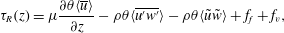 $$\begin{eqnarray}\unicode[STIX]{x1D70F}_{R}(z)=\unicode[STIX]{x1D707}\frac{\unicode[STIX]{x2202}\unicode[STIX]{x1D703}\langle \overline{u}\rangle }{\unicode[STIX]{x2202}z}-\unicode[STIX]{x1D70C}\unicode[STIX]{x1D703}\langle \overline{u^{\prime }w^{\prime }}\rangle -\unicode[STIX]{x1D70C}\unicode[STIX]{x1D703}\langle \tilde{u} \tilde{w}\rangle +f_{f}+f_{v},\end{eqnarray}$$
where
 $u$
,
$u$
,
 $v$
and
$v$
and
 $w$
are the velocity components in the directions of
$w$
are the velocity components in the directions of
 $x$
,
$x$
,
 $y$
and
$y$
and
 $z$
,
$z$
,
 $\unicode[STIX]{x1D70F}_{R}$
is the total force per unit area in the horizontal plane,
$\unicode[STIX]{x1D70F}_{R}$
is the total force per unit area in the horizontal plane,
 $\unicode[STIX]{x1D707}$
the dynamic viscosity and
$\unicode[STIX]{x1D707}$
the dynamic viscosity and
 $\unicode[STIX]{x1D70C}$
the fluid density.
$\unicode[STIX]{x1D70C}$
the fluid density.
 $\unicode[STIX]{x1D703}(z)$
is the porosity function with respect to
$\unicode[STIX]{x1D703}(z)$
is the porosity function with respect to
 $z$
, which takes on a value of 1 above the sediment bed and reaches a constant value
$z$
, which takes on a value of 1 above the sediment bed and reaches a constant value
 $\unicode[STIX]{x1D703}_{p}$
well within the sediment bed. The terms in (2.1) are the viscous stress (
$\unicode[STIX]{x1D703}_{p}$
well within the sediment bed. The terms in (2.1) are the viscous stress (
 $\unicode[STIX]{x1D70F}_{v}$
), turbulent stress (
$\unicode[STIX]{x1D70F}_{v}$
), turbulent stress (
 $\unicode[STIX]{x1D70F}_{t}$
), form-induced stress (
$\unicode[STIX]{x1D70F}_{t}$
), form-induced stress (
 $\unicode[STIX]{x1D70F}_{f}$
), form drag per unit area (
$\unicode[STIX]{x1D70F}_{f}$
), form drag per unit area (
 $f_{f}$
) and viscous drag per unit area (
$f_{f}$
) and viscous drag per unit area (
 $f_{v}$
) respectively. Note that the viscous, turbulent and form-induced stresses represent fluid stresses acting in the fluid domain (the sum defines the total fluid shear stress
$f_{v}$
) respectively. Note that the viscous, turbulent and form-induced stresses represent fluid stresses acting in the fluid domain (the sum defines the total fluid shear stress
 $\unicode[STIX]{x1D70F}$
), while the viscous and form drag represent forces acting at the surfaces of the sediment grains. The fluid stresses relate to a flux of momentum while drag forces relate to the momentum sink. The relevance of each term depends on
$\unicode[STIX]{x1D70F}$
), while the viscous and form drag represent forces acting at the surfaces of the sediment grains. The fluid stresses relate to a flux of momentum while drag forces relate to the momentum sink. The relevance of each term depends on
 $z$
, the properties of the flow and the properties of the boundary.
$z$
, the properties of the flow and the properties of the boundary.
 $f_{f}$
and
$f_{f}$
and
 $f_{v}$
for instance are both zero above the roughness crests of the sediment bed.
$f_{v}$
for instance are both zero above the roughness crests of the sediment bed.
2.2 Permeability Reynolds number
In description of either transport across the SWI or the flow properties above the interface, many different velocity and length scales have been employed. Examples include the velocity at the top of the boundary layer
 $U_{\unicode[STIX]{x1D6FF}}$
, the shear velocity
$U_{\unicode[STIX]{x1D6FF}}$
, the shear velocity
 $u_{\ast }$
, the boundary layer thickness
$u_{\ast }$
, the boundary layer thickness
 $\unicode[STIX]{x1D6FF}$
defined as
$\unicode[STIX]{x1D6FF}$
defined as
 $\langle \overline{u}\rangle _{z=\unicode[STIX]{x1D6FF}}=0.99U_{\infty }$
, the size of the roughness elements
$\langle \overline{u}\rangle _{z=\unicode[STIX]{x1D6FF}}=0.99U_{\infty }$
, the size of the roughness elements
 $k_{s}$
, the square root of the sediment permeability
$k_{s}$
, the square root of the sediment permeability
 $\sqrt{K}$
and the thickness of the porous medium
$\sqrt{K}$
and the thickness of the porous medium
 $H_{s}$
. Thus, a variety of Reynolds numbers have been used to characterise the flow:
$H_{s}$
. Thus, a variety of Reynolds numbers have been used to characterise the flow:
 $Re=U_{\unicode[STIX]{x1D6FF}}\unicode[STIX]{x1D6FF}/\unicode[STIX]{x1D708}$
,
$Re=U_{\unicode[STIX]{x1D6FF}}\unicode[STIX]{x1D6FF}/\unicode[STIX]{x1D708}$
,
 $Re_{\ast }=u_{\ast }\unicode[STIX]{x1D6FF}/\unicode[STIX]{x1D708}$
,
$Re_{\ast }=u_{\ast }\unicode[STIX]{x1D6FF}/\unicode[STIX]{x1D708}$
,
 $Re_{k_{s}}=u_{\ast }k_{s}/\unicode[STIX]{x1D708}$
and the permeability Reynolds number
$Re_{k_{s}}=u_{\ast }k_{s}/\unicode[STIX]{x1D708}$
and the permeability Reynolds number
 $Re_{K}=u_{\ast }\sqrt{K}/\unicode[STIX]{x1D708}$
, where
$Re_{K}=u_{\ast }\sqrt{K}/\unicode[STIX]{x1D708}$
, where
 $\unicode[STIX]{x1D708}$
is the kinematic viscosity. The sediment bed thickness (
$\unicode[STIX]{x1D708}$
is the kinematic viscosity. The sediment bed thickness (
 $H_{s}$
) becomes relevant only when it restricts the depth of flow penetration (e.g. Prinos, Sofialidis & Keramaris Reference Prinos, Sofialidis and Keramaris2003). When this restriction occurs, the boundary is not considered fully permeable and the flow will be strongly dependent on the dimensionless bed thickness,
$H_{s}$
) becomes relevant only when it restricts the depth of flow penetration (e.g. Prinos, Sofialidis & Keramaris Reference Prinos, Sofialidis and Keramaris2003). When this restriction occurs, the boundary is not considered fully permeable and the flow will be strongly dependent on the dimensionless bed thickness,
 $H_{s}/\sqrt{K}$
. Here, we only consider fully permeable boundaries, defined as a boundary for which the depth of penetration of the mean flow and turbulence are independent of
$H_{s}/\sqrt{K}$
. Here, we only consider fully permeable boundaries, defined as a boundary for which the depth of penetration of the mean flow and turbulence are independent of
 $H_{s}$
. Both
$H_{s}$
. Both
 $Re$
and
$Re$
and
 $Re_{\ast }$
characterise the overlying flow and do not take into account the physical properties of the SWI. Both
$Re_{\ast }$
characterise the overlying flow and do not take into account the physical properties of the SWI. Both
 $Re_{k_{s}}$
and
$Re_{k_{s}}$
and
 $Re_{K}$
are dynamically relevant to the flow at the SWI, and both have been used to describe the near-boundary hydrodynamics (e.g. Jiménez Reference Jiménez2004; Breugem, Boersma & Uittenbogaard Reference Breugem, Boersma and Uittenbogaard2006) and enhanced exchange across the SWI (O’Connor & Harvey Reference O’Connor and Harvey2008). For granular beds,
$Re_{K}$
are dynamically relevant to the flow at the SWI, and both have been used to describe the near-boundary hydrodynamics (e.g. Jiménez Reference Jiménez2004; Breugem, Boersma & Uittenbogaard Reference Breugem, Boersma and Uittenbogaard2006) and enhanced exchange across the SWI (O’Connor & Harvey Reference O’Connor and Harvey2008). For granular beds,
 $\sqrt{K}$
and
$\sqrt{K}$
and
 $k_{s}$
are tightly linked (e.g. Wilson, Huettel & Klein Reference Wilson, Huettel and Klein2008). In particular, for a bed composed of monodisperse spherical particles,
$k_{s}$
are tightly linked (e.g. Wilson, Huettel & Klein Reference Wilson, Huettel and Klein2008). In particular, for a bed composed of monodisperse spherical particles,
 $k_{s}/\sqrt{K}\approx 9$
. Moreover, it is argued that as the depth of penetration increases with
$k_{s}/\sqrt{K}\approx 9$
. Moreover, it is argued that as the depth of penetration increases with
 $Re_{K}$
, the roughness length scale seen by the overlying flow increases as well, thereby inextricably linking
$Re_{K}$
, the roughness length scale seen by the overlying flow increases as well, thereby inextricably linking
 $Re_{K}$
and
$Re_{K}$
and
 $Re_{k_{s}}$
(Manes et al.
Reference Manes, Pokrajac, Nikora, Ridolfi and Poggi2011b
; Manes, Ridolfi & Katul Reference Manes, Ridolfi and Katul2012). The relationship between
$Re_{k_{s}}$
(Manes et al.
Reference Manes, Pokrajac, Nikora, Ridolfi and Poggi2011b
; Manes, Ridolfi & Katul Reference Manes, Ridolfi and Katul2012). The relationship between
 $\sqrt{K}$
and
$\sqrt{K}$
and
 $k_{s}$
may be highly variable in other porous media, thus restricting the application of this study to granular beds. As the importance of
$k_{s}$
may be highly variable in other porous media, thus restricting the application of this study to granular beds. As the importance of
 $Re_{K}$
in governing interfacial fluxes of momentum (e.g. Ruff & Gelhar (Reference Ruff and Gelhar1972), Breugem et al. (Reference Breugem, Boersma and Uittenbogaard2006) and implicitly in Manes et al. (Reference Manes, Ridolfi and Katul2012)) and mass (Grant et al.
Reference Grant, Stewardson and Marusic2012) has been clearly identified, and the influence of the roughness elements is implicitly taken into account in
$Re_{K}$
in governing interfacial fluxes of momentum (e.g. Ruff & Gelhar (Reference Ruff and Gelhar1972), Breugem et al. (Reference Breugem, Boersma and Uittenbogaard2006) and implicitly in Manes et al. (Reference Manes, Ridolfi and Katul2012)) and mass (Grant et al.
Reference Grant, Stewardson and Marusic2012) has been clearly identified, and the influence of the roughness elements is implicitly taken into account in
 $Re_{K}$
through the use of
$Re_{K}$
through the use of
 $u_{\ast }$
as the relevant velocity scale (Grant et al.
Reference Grant, Stewardson and Marusic2012),
$u_{\ast }$
as the relevant velocity scale (Grant et al.
Reference Grant, Stewardson and Marusic2012),
 $Re_{K}$
is considered here as the key parameter governing the variation of flow properties across the interface of granular sediment beds.
$Re_{K}$
is considered here as the key parameter governing the variation of flow properties across the interface of granular sediment beds.
The strong correlation between
 $Re_{K}$
and the mass flux across the SWI is demonstrated by the experimental data in figure 1. Here, the diffusivity that describes mass transport at the SWI (
$Re_{K}$
and the mass flux across the SWI is demonstrated by the experimental data in figure 1. Here, the diffusivity that describes mass transport at the SWI (
 $D_{eff}$
) is normalised by the molecular diffusion coefficient of the solute (
$D_{eff}$
) is normalised by the molecular diffusion coefficient of the solute (
 $D$
) and presented as a function of
$D$
) and presented as a function of
 $Re_{K}$
. The data come from the vast dataset of Grant et al. (Reference Grant, Stewardson and Marusic2012), supplemented by a data point from Roy, Huettel & Jorgensen (Reference Roy, Huettel and Jorgensen2004) and measurements from Chandler et al. (Reference Chandler, Guymer, Pearson and van Egmond2016). By assuming a kinematic viscosity of
$Re_{K}$
. The data come from the vast dataset of Grant et al. (Reference Grant, Stewardson and Marusic2012), supplemented by a data point from Roy, Huettel & Jorgensen (Reference Roy, Huettel and Jorgensen2004) and measurements from Chandler et al. (Reference Chandler, Guymer, Pearson and van Egmond2016). By assuming a kinematic viscosity of
 $1\times 10^{-6}~\text{m}^{2}~\text{s}^{-1}$
, curves of constant
$1\times 10^{-6}~\text{m}^{2}~\text{s}^{-1}$
, curves of constant
 $Re_{K}$
can be drawn, showing that mass transfer across the SWI is strongly dependent on
$Re_{K}$
can be drawn, showing that mass transfer across the SWI is strongly dependent on
 $Re_{K}$
. For
$Re_{K}$
. For
 $Re_{K}\leqslant O(0.01)$
, the total rate of mass transport is given by molecular diffusion alone, reflecting the impermeability of the boundary at low
$Re_{K}\leqslant O(0.01)$
, the total rate of mass transport is given by molecular diffusion alone, reflecting the impermeability of the boundary at low
 $Re_{K}$
. Conversely, for
$Re_{K}$
. Conversely, for
 $Re_{K}\geqslant O(0.1)$
, molecular diffusion becomes a negligible contributor to mass transport at the SWI, indicating that other transport mechanisms must dominate interfacial transfer.
$Re_{K}\geqslant O(0.1)$
, molecular diffusion becomes a negligible contributor to mass transport at the SWI, indicating that other transport mechanisms must dominate interfacial transfer.

Figure 1. The dependence of mass transfer at the SWI on
 $Re_{K}$
. The colour of the markers represents the ratio of the effective diffusivity at the SWI to the coefficient of molecular diffusion (
$Re_{K}$
. The colour of the markers represents the ratio of the effective diffusivity at the SWI to the coefficient of molecular diffusion (
 $D_{eff}/D$
); data are taken from Roy et al. (Reference Roy, Huettel and Jorgensen2004), Grant et al. (Reference Grant, Stewardson and Marusic2012) and Chandler et al. (Reference Chandler, Guymer, Pearson and van Egmond2016). Diagonal lines of constant
$D_{eff}/D$
); data are taken from Roy et al. (Reference Roy, Huettel and Jorgensen2004), Grant et al. (Reference Grant, Stewardson and Marusic2012) and Chandler et al. (Reference Chandler, Guymer, Pearson and van Egmond2016). Diagonal lines of constant
 $Re_{K}$
are shown, assuming
$Re_{K}$
are shown, assuming
 $\unicode[STIX]{x1D708}=1\times 10^{-6}~\text{m}^{2}~\text{s}^{-1}$
. Sediment classifications (from Bear Reference Bear1972) are given in grey. A strong correlation exists between interfacial mass transport and
$\unicode[STIX]{x1D708}=1\times 10^{-6}~\text{m}^{2}~\text{s}^{-1}$
. Sediment classifications (from Bear Reference Bear1972) are given in grey. A strong correlation exists between interfacial mass transport and
 $Re_{K}$
; for
$Re_{K}$
; for
 $Re_{K}\geqslant O(0.1)$
, molecular diffusion becomes negligible in interfacial transport.
$Re_{K}\geqslant O(0.1)$
, molecular diffusion becomes negligible in interfacial transport.
The permeability Reynolds number represents the ratio of the sediment permeability scale to the viscous length scale
 $\unicode[STIX]{x1D708}/u_{\ast }$
. A sediment bed of fixed permeability can therefore be considered as either impermeable or permeable, depending on the flow conditions (i.e. the value of
$\unicode[STIX]{x1D708}/u_{\ast }$
. A sediment bed of fixed permeability can therefore be considered as either impermeable or permeable, depending on the flow conditions (i.e. the value of
 $u_{\ast }$
). The two limiting conditions of
$u_{\ast }$
). The two limiting conditions of
 $Re_{K}$
represent (i) an effectively impermeable boundary (i.e.
$Re_{K}$
represent (i) an effectively impermeable boundary (i.e.
 $Re_{K}\ll 1$
) and (ii) a highly permeable boundary (i.e.
$Re_{K}\ll 1$
) and (ii) a highly permeable boundary (i.e.
 $Re_{K}\gg 1$
), where turbulence can penetrate into the interstitial fluid (Breugem et al.
Reference Breugem, Boersma and Uittenbogaard2006). As aquatic sediments typically have permeabilities of
$Re_{K}\gg 1$
), where turbulence can penetrate into the interstitial fluid (Breugem et al.
Reference Breugem, Boersma and Uittenbogaard2006). As aquatic sediments typically have permeabilities of
 $10^{-12}{-}10^{-7}~\text{m}^{2}$
(Rosgen Reference Rosgen1994; Wilson et al.
Reference Wilson, Huettel and Klein2008), and shear velocities of
$10^{-12}{-}10^{-7}~\text{m}^{2}$
(Rosgen Reference Rosgen1994; Wilson et al.
Reference Wilson, Huettel and Klein2008), and shear velocities of
 $0.1{-}10~\text{cm}~\text{s}^{-1}$
, sediment beds in aquatic systems exist in the range
$0.1{-}10~\text{cm}~\text{s}^{-1}$
, sediment beds in aquatic systems exist in the range
 $Re_{K}=O(0.001{-}10)$
. This suggests that the sediment bed in aquatic systems is typically located in a range of important transition between the impermeable and fully permeable boundary flow regimes.
$Re_{K}=O(0.001{-}10)$
. This suggests that the sediment bed in aquatic systems is typically located in a range of important transition between the impermeable and fully permeable boundary flow regimes.
2.3 Flow characteristics for
 $Re_{K}\ll 1$

Flows bounded by an impermeable boundary, either smooth or rough, are characterised by the no-slip condition at the wall and the shear force at the impermeable boundary is given by the sum of the form and the viscous drag of the roughness elements, i.e.
 $\unicode[STIX]{x1D70F}_{R}(z=0)=f_{f}+f_{v}$
(2.1). Further away from the wall, the effects of turbulence grow and turbulent length scales are limited only by the distance from the wall, leading to the classical logarithmic velocity profile (figure 2
a). This depiction is a simplification of the complex nature of turbulence in impermeable boundary layer flows; for example, the viscosity-dominated near-wall region is not completely independent of the effects of turbulent structures in the outer region (e.g. Marusic, Mathis & Hutchins Reference Marusic, Mathis and Hutchins2010) and quasi-periodic packets transport low momentum fluid into the outer region and high momentum fluid to the near-wall region (e.g. Adrian, Meinhart & Tomkins Reference Adrian, Meinhart and Tomkins2000). The impermeability of the wall has a substantial influence on the near-wall transport of energy, as turbulent fluctuations into the wall (i.e. sweeps) are redirected into wall-tangent components due to the inability of the flow to penetrate the wall. This is referred to as the ‘wall-blocking effect’ (Perot & Moin Reference Perot and Moin1995).
$\unicode[STIX]{x1D70F}_{R}(z=0)=f_{f}+f_{v}$
(2.1). Further away from the wall, the effects of turbulence grow and turbulent length scales are limited only by the distance from the wall, leading to the classical logarithmic velocity profile (figure 2
a). This depiction is a simplification of the complex nature of turbulence in impermeable boundary layer flows; for example, the viscosity-dominated near-wall region is not completely independent of the effects of turbulent structures in the outer region (e.g. Marusic, Mathis & Hutchins Reference Marusic, Mathis and Hutchins2010) and quasi-periodic packets transport low momentum fluid into the outer region and high momentum fluid to the near-wall region (e.g. Adrian, Meinhart & Tomkins Reference Adrian, Meinhart and Tomkins2000). The impermeability of the wall has a substantial influence on the near-wall transport of energy, as turbulent fluctuations into the wall (i.e. sweeps) are redirected into wall-tangent components due to the inability of the flow to penetrate the wall. This is referred to as the ‘wall-blocking effect’ (Perot & Moin Reference Perot and Moin1995).

Figure 2. Framework identifying flow at the SWI (b) as a transition between flows over impermeable boundaries (a) and highly permeable boundaries (c). The variation of the structure of the mean flow and turbulence with
 $Re_{K}$
is shown schematically.
$Re_{K}$
is shown schematically.
2.4 Flow characteristics for
$Re_{K}\gg 1$

The interface of a highly permeable boundary connects a region of velocity deficit within the permeable layer to a free stream region above the interface. The interface is characterised by a distinct inflection point in the streamwise velocity profile (figure 2
c) and is typically associated with the presence of a Kelvin–Helmholtz-type (KH) instability (Raupach, Finnigan & Brunei Reference Raupach, Finnigan and Brunei1996). This instability leads to the development of coherent turbulent structures with a predictable frequency, corresponding to the natural frequency of instability of the hyperbolic tangent mixing layer velocity profile (Ho & Huerre Reference Ho and Huerre1984). Unlike the broad range of turbulent time and length scales found in the impermeable boundary layer, the interface region is dominated by the single scale of these structures. These structures create much more efficient vertical mixing than those in an impermeable boundary layer flow (Ghisalberti & Nepf Reference Ghisalberti and Nepf2002; Ghisalberti Reference Ghisalberti2009). As the high permeability allows turbulent structures to penetrate the interface, the transport of mass across the interface is dominated by turbulent transport. Unlike the impermeable boundary layer flow, the interfacial shear force is now dominated by the Reynolds stress, with a small contribution from the form-induced stress
 $\unicode[STIX]{x1D70F}_{R}(z=0)\simeq -\unicode[STIX]{x1D70C}\unicode[STIX]{x1D703}\langle \overline{u^{\prime }w^{\prime }}\rangle -\unicode[STIX]{x1D70C}\unicode[STIX]{x1D703}\langle \tilde{u} \tilde{w}\rangle +f_{f}$
.
$\unicode[STIX]{x1D70F}_{R}(z=0)\simeq -\unicode[STIX]{x1D70C}\unicode[STIX]{x1D703}\langle \overline{u^{\prime }w^{\prime }}\rangle -\unicode[STIX]{x1D70C}\unicode[STIX]{x1D703}\langle \tilde{u} \tilde{w}\rangle +f_{f}$
.
Although the physical appearance of highly permeable media (e.g. urban canopies, submerged vegetation and coral reefs) can vary dramatically, they are all characterised by a drag-induced inflection point in the vertical profile of the mean velocity. The dominance of KH-type turbulent structures in this region engenders a similarity in flows across permeable boundaries at high
 $Re_{K}$
; this similarity is seen in properties such as the depth of penetration of shear into the porous medium, the interfacial velocity (
$Re_{K}$
; this similarity is seen in properties such as the depth of penetration of shear into the porous medium, the interfacial velocity (
 $U_{i}=\langle \overline{u}\rangle _{z=0}$
) and the turbulence anisotropy at the interface (Ghisalberti Reference Ghisalberti2009). This similarity implies that interfacial properties become independent of permeability for
$U_{i}=\langle \overline{u}\rangle _{z=0}$
) and the turbulence anisotropy at the interface (Ghisalberti Reference Ghisalberti2009). This similarity implies that interfacial properties become independent of permeability for
 $Re_{K}\gg 1$
. Note, however, that this behaviour does not hold for a continuous increase of the permeability, as the flow typology will eventually revert to that of a classical turbulent impermeable boundary layer (Poggi et al.
Reference Poggi, Porporato, Ridolfi, Albertson and Katul2004). For these ‘thickness-limited permeable boundaries’, where the penetration depth of the flow is constrained by the finite thickness of the permeable medium, other non-dimensional numbers, such as
$Re_{K}\gg 1$
. Note, however, that this behaviour does not hold for a continuous increase of the permeability, as the flow typology will eventually revert to that of a classical turbulent impermeable boundary layer (Poggi et al.
Reference Poggi, Porporato, Ridolfi, Albertson and Katul2004). For these ‘thickness-limited permeable boundaries’, where the penetration depth of the flow is constrained by the finite thickness of the permeable medium, other non-dimensional numbers, such as
 $\sqrt{K}/H_{s}$
, become relevant.
$\sqrt{K}/H_{s}$
, become relevant.
2.5 Flow characteristics for
$Re_{K}\sim O(1)$

The dynamics of transitional
 $Re_{K}$
flows have remained largely undocumented as technical limitations complicate the acquisition of detailed flow observations across the interface. Consequently, much of the current understanding comes from experimental measurement of dynamics either above the interface or from numerical simulations. As suggested in figure 2(b), the mean velocity profile over a large range of
$Re_{K}$
flows have remained largely undocumented as technical limitations complicate the acquisition of detailed flow observations across the interface. Consequently, much of the current understanding comes from experimental measurement of dynamics either above the interface or from numerical simulations. As suggested in figure 2(b), the mean velocity profile over a large range of
 $Re_{K}$
possesses characteristics of both the impermeable boundary and the highly permeable boundary, with a logarithmic velocity profile above the interface (e.g. Suga et al.
Reference Suga, Matsumura, Ashitaka, Tominaga and Kaneda2010; Manes, Poggi & Ridolfi Reference Manes, Poggi and Ridolfi2011a
) and an inflection point at the interface (e.g. Goharzadeh, Khalili & Jørgensen Reference Goharzadeh, Khalili and Jørgensen2005; Breugem et al.
Reference Breugem, Boersma and Uittenbogaard2006). Similarly to the highly permeable boundary, a shear layer develops below the SWI, reaching a constant mean velocity (
$Re_{K}$
possesses characteristics of both the impermeable boundary and the highly permeable boundary, with a logarithmic velocity profile above the interface (e.g. Suga et al.
Reference Suga, Matsumura, Ashitaka, Tominaga and Kaneda2010; Manes, Poggi & Ridolfi Reference Manes, Poggi and Ridolfi2011a
) and an inflection point at the interface (e.g. Goharzadeh, Khalili & Jørgensen Reference Goharzadeh, Khalili and Jørgensen2005; Breugem et al.
Reference Breugem, Boersma and Uittenbogaard2006). Similarly to the highly permeable boundary, a shear layer develops below the SWI, reaching a constant mean velocity (
 $U_{p}=\langle \overline{u}\rangle _{z<-\unicode[STIX]{x1D6FF}_{b}}$
) at a distance
$U_{p}=\langle \overline{u}\rangle _{z<-\unicode[STIX]{x1D6FF}_{b}}$
) at a distance
 $\unicode[STIX]{x1D6FF}_{b}$
below the interface. This depth of penetration is referred to as the Brinkman layer thickness,
$\unicode[STIX]{x1D6FF}_{b}$
below the interface. This depth of penetration is referred to as the Brinkman layer thickness,
 $\unicode[STIX]{x1D6FF}_{b}$
, a crucial parameter in slip models, and is argued to be proportional to the square root of the permeability or the representative grain diameter, i.e.
$\unicode[STIX]{x1D6FF}_{b}$
, a crucial parameter in slip models, and is argued to be proportional to the square root of the permeability or the representative grain diameter, i.e.
 $\unicode[STIX]{x1D6FF}_{b}\propto \sqrt{K}$
or
$\unicode[STIX]{x1D6FF}_{b}\propto \sqrt{K}$
or
 $\unicode[STIX]{x1D6FF}_{b}\propto d$
(e.g. Boudreau Reference Boudreau2001; Goyeau et al.
Reference Goyeau, Lhuillier, Gobin and Velarde2003; Goharzadeh et al.
Reference Goharzadeh, Khalili and Jørgensen2005).
$\unicode[STIX]{x1D6FF}_{b}\propto d$
(e.g. Boudreau Reference Boudreau2001; Goyeau et al.
Reference Goyeau, Lhuillier, Gobin and Velarde2003; Goharzadeh et al.
Reference Goharzadeh, Khalili and Jørgensen2005).
As the permeability of the SWI allows for flow penetration into the porous medium, the interfacial velocity is non-zero. The interfacial velocity at the SWI has been suggested to be a function of the shear velocity
 $u_{\ast }$
for
$u_{\ast }$
for
 $Re_{K}=O(0.1{-}1)$
(Suga et al.
Reference Suga, Matsumura, Ashitaka, Tominaga and Kaneda2010). Although a clear understanding of the variation of
$Re_{K}=O(0.1{-}1)$
(Suga et al.
Reference Suga, Matsumura, Ashitaka, Tominaga and Kaneda2010). Although a clear understanding of the variation of
 $U_{i}/u_{\ast }$
with
$U_{i}/u_{\ast }$
with
 $Re_{K}$
is desirable, the sensitivity of
$Re_{K}$
is desirable, the sensitivity of
 $U_{i}$
to the choice of position of the interface makes determination of
$U_{i}$
to the choice of position of the interface makes determination of
 $U_{i}/u_{\ast }$
difficult. For instance, in some studies the SWI is taken at the absolute top of the obstructive elements (e.g. Goharzadeh et al.
Reference Goharzadeh, Khalili and Jørgensen2005; Breugem et al.
Reference Breugem, Boersma and Uittenbogaard2006; Suga et al.
Reference Suga, Matsumura, Ashitaka, Tominaga and Kaneda2010), which typically corresponds to the definition in highly permeable boundaries (Nepf Reference Nepf2012). However, others adopt a definition closer to that of an impermeable boundary, positioning the interface within the roughness elements (e.g. Nezu & Nakagawa Reference Nezu and Nakagawa1993; Nikora et al.
Reference Nikora, Goring, McEwan and Griffiths2001). This links the interface position to the physical length scale of the roughness elements at the interface which, in the case of a flat sediment bed, is the characteristic grain diameter.
$U_{i}/u_{\ast }$
difficult. For instance, in some studies the SWI is taken at the absolute top of the obstructive elements (e.g. Goharzadeh et al.
Reference Goharzadeh, Khalili and Jørgensen2005; Breugem et al.
Reference Breugem, Boersma and Uittenbogaard2006; Suga et al.
Reference Suga, Matsumura, Ashitaka, Tominaga and Kaneda2010), which typically corresponds to the definition in highly permeable boundaries (Nepf Reference Nepf2012). However, others adopt a definition closer to that of an impermeable boundary, positioning the interface within the roughness elements (e.g. Nezu & Nakagawa Reference Nezu and Nakagawa1993; Nikora et al.
Reference Nikora, Goring, McEwan and Griffiths2001). This links the interface position to the physical length scale of the roughness elements at the interface which, in the case of a flat sediment bed, is the characteristic grain diameter.
An inflection point in the mean velocity profile, characteristic of highly permeable boundary flows, exists (even at low
 $Re_{K}$
) at the SWI (Goharzadeh et al.
Reference Goharzadeh, Khalili and Jørgensen2005). Because of this inflection point, linear stability analysis suggests that flow over a porous medium of any non-zero porosity is unstable (White & Nepf Reference White and Nepf2007). The existence of these KH-type coherent structures at the SWI at high
$Re_{K}$
) at the SWI (Goharzadeh et al.
Reference Goharzadeh, Khalili and Jørgensen2005). Because of this inflection point, linear stability analysis suggests that flow over a porous medium of any non-zero porosity is unstable (White & Nepf Reference White and Nepf2007). The existence of these KH-type coherent structures at the SWI at high
 $Re_{K}$
(where they cannot be damped by viscosity) has been hypothesised by Breugem et al. (Reference Breugem, Boersma and Uittenbogaard2006) and Suga, Mori & Kaneda (Reference Suga, Mori and Kaneda2011) based on two-dimensional snap shots of the interfacial flow field. Experimental evidence of their existence, however, remains sparse (e.g. Manes et al.
Reference Manes, Poggi and Ridolfi2011a
), with no experimental evidence for the existence of KH instabilities at the SWI for granular beds. This suggests that an inflectional velocity profile in these systems is a result of the drag induced by the porous medium and not necessarily indicative of an inflectional instability.
$Re_{K}$
(where they cannot be damped by viscosity) has been hypothesised by Breugem et al. (Reference Breugem, Boersma and Uittenbogaard2006) and Suga, Mori & Kaneda (Reference Suga, Mori and Kaneda2011) based on two-dimensional snap shots of the interfacial flow field. Experimental evidence of their existence, however, remains sparse (e.g. Manes et al.
Reference Manes, Poggi and Ridolfi2011a
), with no experimental evidence for the existence of KH instabilities at the SWI for granular beds. This suggests that an inflectional velocity profile in these systems is a result of the drag induced by the porous medium and not necessarily indicative of an inflectional instability.
As
 $Re_{K}$
increases, the flow is able to penetrate the interface, weakening the wall-blocking effect. The relative intensity of the vertical velocity fluctuations therefore increases while the intensity of the streamwise fluctuations decreases (Breugem et al.
Reference Breugem, Boersma and Uittenbogaard2006; Suga et al.
Reference Suga, Matsumura, Ashitaka, Tominaga and Kaneda2010; Manes et al.
Reference Manes, Poggi and Ridolfi2011a
), enhancing mass transfer (as seen in figure 1). The observed decrease in streamwise turbulence intensity near the interface is most likely related to a change in turbulent structures in the near-wall region, as Breugem et al. (Reference Breugem, Boersma and Uittenbogaard2006) found that the signatures of the large-scale motions, typical for the impermeable boundary, disappear for
$Re_{K}$
increases, the flow is able to penetrate the interface, weakening the wall-blocking effect. The relative intensity of the vertical velocity fluctuations therefore increases while the intensity of the streamwise fluctuations decreases (Breugem et al.
Reference Breugem, Boersma and Uittenbogaard2006; Suga et al.
Reference Suga, Matsumura, Ashitaka, Tominaga and Kaneda2010; Manes et al.
Reference Manes, Poggi and Ridolfi2011a
), enhancing mass transfer (as seen in figure 1). The observed decrease in streamwise turbulence intensity near the interface is most likely related to a change in turbulent structures in the near-wall region, as Breugem et al. (Reference Breugem, Boersma and Uittenbogaard2006) found that the signatures of the large-scale motions, typical for the impermeable boundary, disappear for
 $Re_{K}\gtrsim 1$
. Suga et al. (Reference Suga, Mori and Kaneda2011) observed similar changes above the interface for flow over porous foam, where packets of hairpin vortices become unidentifiable at higher values of
$Re_{K}\gtrsim 1$
. Suga et al. (Reference Suga, Mori and Kaneda2011) observed similar changes above the interface for flow over porous foam, where packets of hairpin vortices become unidentifiable at higher values of
 $Re_{K}$
. This suggests that the turbulent structures typically found in impermeable boundary layer flow gradually disappear with increasing
$Re_{K}$
. This suggests that the turbulent structures typically found in impermeable boundary layer flow gradually disappear with increasing
 $Re_{K}$
. The weakening of the wall-blocking effect and the ability of both the mean flow and turbulence to penetrate the interface suggest that none of the terms in (2.1) can be neglected a priori in determining the total shear force (including both fluid stresses and drag at the bed surface) at the interface.
$Re_{K}$
. The weakening of the wall-blocking effect and the ability of both the mean flow and turbulence to penetrate the interface suggest that none of the terms in (2.1) can be neglected a priori in determining the total shear force (including both fluid stresses and drag at the bed surface) at the interface.
While the framework presented here is consistent with a broad range of studies, it cannot be quantified without experimental measurement of the mean and turbulent flow at the SWI. This experimental study provides these measurements. In this work, we focus on two key issues: (i) demonstrating that the hydrodynamics at the SWI indeed represent a transitional regime that couples two canonical flow typologies (the impermeable boundary and the highly permeable boundary flow) and (ii) that the flow properties at the SWI in this transitional regime are strongly dependent on
 $Re_{K}$
. These observations and this framework are then used to examine the implications for descriptions of interfacial transport in flows over sediment beds.
$Re_{K}$
. These observations and this framework are then used to examine the implications for descriptions of interfacial transport in flows over sediment beds.
3 Methodology
Laboratory experiments were conducted in a 2-m-long glass-walled flume with a cross-sectional area of
 $0.4\times 0.4~\text{m}^{2}$
(figure 3). Fluid was recirculated by a centrifugal pump and the discharge adjusted by changing the rotational speed of the pump. A false bottom was used at each end of the flume, creating a rectangular void of length
$0.4\times 0.4~\text{m}^{2}$
(figure 3). Fluid was recirculated by a centrifugal pump and the discharge adjusted by changing the rotational speed of the pump. A false bottom was used at each end of the flume, creating a rectangular void of length
 $L=1.10~\text{m}$
and height
$L=1.10~\text{m}$
and height
 $H_{S}=0.15~\text{m}$
. The space was randomly filled with monodisperse borosilicate glass spheres to represent a horizontal sediment bed. Sphere diameters of 6 mm, 10 mm and 25 mm were used (referred to as ‘small’ (S), ‘medium’ (M) and ‘large’ (L), respectively). The depth of fluid above the bed at
$H_{S}=0.15~\text{m}$
. The space was randomly filled with monodisperse borosilicate glass spheres to represent a horizontal sediment bed. Sphere diameters of 6 mm, 10 mm and 25 mm were used (referred to as ‘small’ (S), ‘medium’ (M) and ‘large’ (L), respectively). The depth of fluid above the bed at
 $x=0$
(
$x=0$
(
 $H$
) was kept constant at 9 cm, with a free surface gradient driving the flow. Flow disturbances originating from the inlet were dampened by a combination of porous foam and flow straighteners. The directions of
$H$
) was kept constant at 9 cm, with a free surface gradient driving the flow. Flow disturbances originating from the inlet were dampened by a combination of porous foam and flow straighteners. The directions of
 $x$
,
$x$
,
 $y$
and
$y$
and
 $z$
, with velocity components in those directions given by
$z$
, with velocity components in those directions given by
 $u$
,
$u$
,
 $v$
and
$v$
and
 $w$
, are shown in figure 3; the origin is located at the SWI at the leading edge of the sediment bed. The technical difficulties of acquiring detailed measurements across the SWI were overcome here by combining particle tracking velocimetry (PTV) with refractive index matching (RIM).
$w$
, are shown in figure 3; the origin is located at the SWI at the leading edge of the sediment bed. The technical difficulties of acquiring detailed measurements across the SWI were overcome here by combining particle tracking velocimetry (PTV) with refractive index matching (RIM).

Figure 3. Experimental set-up of the recirculating flume. The flow is driven by a centrifugal pump and has a fixed depth of
 $H=9$
cm. The model sediment bed, consisting of monodisperse borosilicate glass beads, has a height
$H=9$
cm. The model sediment bed, consisting of monodisperse borosilicate glass beads, has a height
 $H_{s}=15$
cm and a length
$H_{s}=15$
cm and a length
 $L=1.1$
m.
$L=1.1$
m.
3.1 Refractive index matching
RIM was used here to create an unobstructed view into the interstitial fluid. It has previously been applied to obtain information about the hydrodynamics in obstructed systems, such as at the SWI (Goharzadeh et al.
Reference Goharzadeh, Khalili and Jørgensen2005), in canopy flow (Bai, Katz & Meneveau Reference Bai, Katz and Meneveau2015) and in mechanical systems (Uzol et al.
Reference Uzol, Chow, Katz and Meneveau2002). The fluid chosen was a 59 % by mass sodium iodide (NaI) solution. The fluid had a specific gravity of 1.77 (measured with an Anton Paar DMA500 density meter) and a kinematic viscosity of
 $1.35\times 10^{-6}~\text{m}^{2}~\text{s}^{-1}$
(measured with a Cannon–Fenske viscometer tube). Importantly, the fluid had a refractive index of
$1.35\times 10^{-6}~\text{m}^{2}~\text{s}^{-1}$
(measured with a Cannon–Fenske viscometer tube). Importantly, the fluid had a refractive index of
 $n=1.4750$
(measured with an Atago pocket refractometer) for a wavelength (
$n=1.4750$
(measured with an Atago pocket refractometer) for a wavelength (
 $\unicode[STIX]{x1D706}$
) of 650 nm at a temperature (
$\unicode[STIX]{x1D706}$
) of 650 nm at a temperature (
 $T$
) of
$T$
) of
 $23\,^{\circ }\text{C}$
. This matches the refractive index of borosilicate glass, the material of the model sediment grains. Figure 4 shows the borosilicate glass beads submerged in NaI solutions of increasing concentration: water, 50 % NaI solution and a 59 % NaI solution. As light was not refracted when both the fluid and the glass have the same refractive index, an undistorted image under the beads becomes visible in the 59 % solution (figure 4
c). Because the refractive index of the solution is a function of temperature, the fluid temperature was kept at
$23\,^{\circ }\text{C}$
. This matches the refractive index of borosilicate glass, the material of the model sediment grains. Figure 4 shows the borosilicate glass beads submerged in NaI solutions of increasing concentration: water, 50 % NaI solution and a 59 % NaI solution. As light was not refracted when both the fluid and the glass have the same refractive index, an undistorted image under the beads becomes visible in the 59 % solution (figure 4
c). Because the refractive index of the solution is a function of temperature, the fluid temperature was kept at
 $23.0\pm 0.8\,^{\circ }\text{C}$
; this ensured that the refractive index of the fluid was maintained within the range
$23.0\pm 0.8\,^{\circ }\text{C}$
; this ensured that the refractive index of the fluid was maintained within the range
 $n=1.4750\pm 0.0002$
(for
$n=1.4750\pm 0.0002$
(for
 $\unicode[STIX]{x1D706}=650$
nm). Although a yellowing of NaI solutions due to oxidation has been previously reported, this only creates absorption of the low wavelength range of the visible spectrum, i.e.
$\unicode[STIX]{x1D706}=650$
nm). Although a yellowing of NaI solutions due to oxidation has been previously reported, this only creates absorption of the low wavelength range of the visible spectrum, i.e.
 $\unicode[STIX]{x1D706}<600$
nm (Uzol et al.
Reference Uzol, Chow, Katz and Meneveau2002; Häfeli et al.
Reference Häfeli, Altheimer, Butscher and von Rohr2014), while the laser light used in these experiments had a wavelength of 650 nm.
$\unicode[STIX]{x1D706}<600$
nm (Uzol et al.
Reference Uzol, Chow, Katz and Meneveau2002; Häfeli et al.
Reference Häfeli, Altheimer, Butscher and von Rohr2014), while the laser light used in these experiments had a wavelength of 650 nm.

Figure 4. The refractive index matching combination of fluid and model sediment used in this study. Shown are borosilicate glass beads in (a) water, (b) 50 % NaI solution, (c) 59 % NaI solution. As the refractive index of the glass beads and the fluid are equal in (c), the image underneath the fluid remains undistorted. The 59 % NaI solution was used in experiments.
3.2 Particle tracking velocimetry
Two-dimensional instantaneous velocity fields were gathered by means of PTV, a measurement technique successfully applied in similar experiments looking at turbulent boundary layer flow (e.g. Cowen & Monismith Reference Cowen and Monismith1997) and flow within a gravel bed pore (Detert et al.
Reference Detert, Klar, Wenka and Jirka2007). Raw images of illuminated tracer particles in the flow were captured by a CCD (charge-coupled device) camera at a rate of 23 frames per second, where a single frame contains
 $2448\times 1200$
px. Two sizes of custom-made silver coated PMMA (Polymethyl methacrylate) particles were used, with diameters of
$2448\times 1200$
px. Two sizes of custom-made silver coated PMMA (Polymethyl methacrylate) particles were used, with diameters of
 $32{-}40~\unicode[STIX]{x03BC}\text{m}$
and
$32{-}40~\unicode[STIX]{x03BC}\text{m}$
and
 $91{-}100~\unicode[STIX]{x03BC}\text{m}$
(and specific gravities of 1.75 and 1.73, respectively). The imaged diameter of the tracer particles, which is greater than the actual tracer particle diameter, was equivalent to 2.0 px, as suggested by Cowen & Monismith (Reference Cowen and Monismith1997). The tracer particles were illuminated by a 1–3 mm thick laser sheet (650 nm wavelength) from two aligned 50 mW lasers with a
$91{-}100~\unicode[STIX]{x03BC}\text{m}$
(and specific gravities of 1.75 and 1.73, respectively). The imaged diameter of the tracer particles, which is greater than the actual tracer particle diameter, was equivalent to 2.0 px, as suggested by Cowen & Monismith (Reference Cowen and Monismith1997). The tracer particles were illuminated by a 1–3 mm thick laser sheet (650 nm wavelength) from two aligned 50 mW lasers with a
 $60^{\circ }$
fan angle Powell lens. The field of view was approximately
$60^{\circ }$
fan angle Powell lens. The field of view was approximately
 $35\times 70$
mm or
$35\times 70$
mm or
 $90\times 180$
mm, depending on the size of the tracer particles. The experimental set-up depended on the sediment grain size, as summarised in table 1.
$90\times 180$
mm, depending on the size of the tracer particles. The experimental set-up depended on the sediment grain size, as summarised in table 1.
Table 1. Details of the experimental set-up for the different sediment sizes.
The optimal particle seeding density for PTV is suggested to be 5–20 particles per
 $32\times 32$
px (Cowen & Monismith Reference Cowen and Monismith1997). This density, however, could not be achieved in our experiments, as tracer particles slowly accumulate in the interstitial fluid and settle on the glass beads. This settling blocks light within the sediments from reaching the camera and hence affects the measurability of the flow field around the SWI. Therefore the seeding density employed was approximately 1 particle per
$32\times 32$
px (Cowen & Monismith Reference Cowen and Monismith1997). This density, however, could not be achieved in our experiments, as tracer particles slowly accumulate in the interstitial fluid and settle on the glass beads. This settling blocks light within the sediments from reaching the camera and hence affects the measurability of the flow field around the SWI. Therefore the seeding density employed was approximately 1 particle per
 $32\times 32$
px. The errors due to the lower seeding densities were expected to be small, as PTV is unaffected by displacement gradients (Cowen & Monismith Reference Cowen and Monismith1997). The measurements provided, on average, a data point every
$32\times 32$
px. The errors due to the lower seeding densities were expected to be small, as PTV is unaffected by displacement gradients (Cowen & Monismith Reference Cowen and Monismith1997). The measurements provided, on average, a data point every
 $4.3\pm 0.9$
mm for the larger tracer particles and
$4.3\pm 0.9$
mm for the larger tracer particles and
 $1.5\pm 0.2$
mm for the smaller tracer particles. Images were taken over a period of 8.75 min in each flow and processed in Matlab to enhance contrast and remove the average background. The optimised images were converted to particle fields in the PTV software Streams (Nokes Reference Nokes2016). Coarse velocity fields were first estimated based on the cross-correlation of particle locations in consecutive frames. Subsequently, detailed Lagrangian path fields were determined using the local velocity and acceleration of this coarse velocity field to match individual particles in multiple consecutive frames. The Lagrangian velocity information was then used to determine a grid-based Eulerian velocity field by triangular interpolation of the neighbouring tracked particles around a grid point. The grid has a resolution of 0.8 mm for the 6 and 10 mm grain diameters and 2.0 mm for the 25 mm grain diameter. This is of the same order as the tracer particle spacing but an order of magnitude smaller than the grain diameters.
$1.5\pm 0.2$
mm for the smaller tracer particles. Images were taken over a period of 8.75 min in each flow and processed in Matlab to enhance contrast and remove the average background. The optimised images were converted to particle fields in the PTV software Streams (Nokes Reference Nokes2016). Coarse velocity fields were first estimated based on the cross-correlation of particle locations in consecutive frames. Subsequently, detailed Lagrangian path fields were determined using the local velocity and acceleration of this coarse velocity field to match individual particles in multiple consecutive frames. The Lagrangian velocity information was then used to determine a grid-based Eulerian velocity field by triangular interpolation of the neighbouring tracked particles around a grid point. The grid has a resolution of 0.8 mm for the 6 and 10 mm grain diameters and 2.0 mm for the 25 mm grain diameter. This is of the same order as the tracer particle spacing but an order of magnitude smaller than the grain diameters.
3.3 Experimental conditions
An overview of the hydrodynamic conditions of the experiments is given in table 2, where the bulk velocity is defined as
 $U_{b}=(1/\unicode[STIX]{x1D6FF})\int _{0}^{\unicode[STIX]{x1D6FF}}\unicode[STIX]{x1D703}\langle \overline{u}\rangle \,\text{d}z$
. Three different sediment sizes were used; with the variation of the shear velocity
$U_{b}=(1/\unicode[STIX]{x1D6FF})\int _{0}^{\unicode[STIX]{x1D6FF}}\unicode[STIX]{x1D703}\langle \overline{u}\rangle \,\text{d}z$
. Three different sediment sizes were used; with the variation of the shear velocity
 $u_{\ast }$
, this allowed a large experimental range of
$u_{\ast }$
, this allowed a large experimental range of
 $Re_{K}$
. The permeability of the sediments
$Re_{K}$
. The permeability of the sediments
 $K$
was estimated using the Carman–Kozeny model:
$K$
was estimated using the Carman–Kozeny model:
 $$\begin{eqnarray}K=\frac{\unicode[STIX]{x1D703}_{p}^{3}}{180(1-\unicode[STIX]{x1D703}_{p})^{2}}d^{2},\end{eqnarray}$$
where
 $d$
is the grain diameter. The porosity
$d$
is the grain diameter. The porosity
 $\unicode[STIX]{x1D703}_{p}$
was determined by measuring the volume of the interstitial fluid in the flume, yielding
$\unicode[STIX]{x1D703}_{p}$
was determined by measuring the volume of the interstitial fluid in the flume, yielding
 $\unicode[STIX]{x1D703}_{p}=0.41$
for all three cases. Although the diameters of the sediments do not correspond to typical sediment sizes in aquatic systems, the range of
$\unicode[STIX]{x1D703}_{p}=0.41$
for all three cases. Although the diameters of the sediments do not correspond to typical sediment sizes in aquatic systems, the range of
 $Re_{K}$
in these experiments was 0.36–6.3 (table 2), which is typical of the values for sediments in real aquatic systems.
$Re_{K}$
in these experiments was 0.36–6.3 (table 2), which is typical of the values for sediments in real aquatic systems.
Table 2. Hydrodynamic properties of the experimental cases.

As the sediment bed had a finite length, it was necessary to determine the point beyond which there was no further evolution of the mean and turbulent velocity flow structure at the SWI. To determine this point, 11 PTV measurements along a streamwise transect were taken in case M7 (table 2). The flow statistics 20 mm above the SWI along this transect are shown in figure 5, where they are normalised by the spatially averaged statistics in the range
 $700<x<800~\text{mm}$
(where
$700<x<800~\text{mm}$
(where
 $x=0$
corresponds to the leading edge of the sediment bed). The statistics are horizontally averaged over intervals of 30 mm. The streamwise velocity
$x=0$
corresponds to the leading edge of the sediment bed). The statistics are horizontally averaged over intervals of 30 mm. The streamwise velocity
 $\langle \overline{u}\rangle$
, the turbulence intensities
$\langle \overline{u}\rangle$
, the turbulence intensities
 $\unicode[STIX]{x1D70E}_{u}=\langle \overline{{u^{\prime }}^{2}}\rangle ^{1/2}$
and
$\unicode[STIX]{x1D70E}_{u}=\langle \overline{{u^{\prime }}^{2}}\rangle ^{1/2}$
and
 $\unicode[STIX]{x1D70E}_{w}=\langle \overline{{w^{\prime }}^{2}}\rangle ^{1/2}$
and the Reynolds stress
$\unicode[STIX]{x1D70E}_{w}=\langle \overline{{w^{\prime }}^{2}}\rangle ^{1/2}$
and the Reynolds stress
 $\langle \overline{u^{\prime }w^{\prime }}\rangle$
along this transect do not change beyond
$\langle \overline{u^{\prime }w^{\prime }}\rangle$
along this transect do not change beyond
 $x=600$
mm (figure 5). Therefore, the measurement location was centred around
$x=600$
mm (figure 5). Therefore, the measurement location was centred around
 $x=750$
mm, by which point there is no further evolution of the interfacial flow. At this position, the boundary layer thickness
$x=750$
mm, by which point there is no further evolution of the interfacial flow. At this position, the boundary layer thickness
 $\unicode[STIX]{x1D6FF}$
for case M7 was measured as 41 mm, which is reasonably close to the predicted flat plate value of 35 mm (see Schlichting (Reference Schlichting1979, p. 638)). This small difference in
$\unicode[STIX]{x1D6FF}$
for case M7 was measured as 41 mm, which is reasonably close to the predicted flat plate value of 35 mm (see Schlichting (Reference Schlichting1979, p. 638)). This small difference in
 $\unicode[STIX]{x1D6FF}$
can be explained by the destabilising effect of wall permeability (Tilton & Cortelezzi Reference Tilton and Cortelezzi2008), which allows a wall-normal velocity component at the interface.
$\unicode[STIX]{x1D6FF}$
can be explained by the destabilising effect of wall permeability (Tilton & Cortelezzi Reference Tilton and Cortelezzi2008), which allows a wall-normal velocity component at the interface.

Figure 5. Flow statistics along a longitudinal transect 20 mm above the SWI:
 $\langle \overline{u}\rangle$
(○),
$\langle \overline{u}\rangle$
(○),
 $\unicode[STIX]{x1D70E}_{u}$
(▫),
$\unicode[STIX]{x1D70E}_{u}$
(▫),
 $\unicode[STIX]{x1D70E}_{w}$
(▿),
$\unicode[STIX]{x1D70E}_{w}$
(▿),
 $\langle \overline{u^{\prime }w^{\prime }}\rangle$
(▵). The statistics are normalised by the average value in the range
$\langle \overline{u^{\prime }w^{\prime }}\rangle$
(▵). The statistics are normalised by the average value in the range
 $700<x<800$
mm, where
$700<x<800$
mm, where
 $x=0$
corresponds to the leading edge of the sediment bed. Fully developed flow at the interface is reached by
$x=0$
corresponds to the leading edge of the sediment bed. Fully developed flow at the interface is reached by
 $x=600$
mm.
$x=600$
mm.
Due to the strong spatial variability of flows over porous media, measurements were taken at three lateral positions to obtain horizontally averaged statistics of the flow properties across the SWI. The lateral measurement positions were at 65 mm, 95 mm and 115 mm from the centreline of the flume (closer to the flume wall nearer the camera). Six measurements of the flow field were recorded in each case. At each of the three lateral positions the camera frame was orientated: (i) horizontally in the
 $x$
–
$x$
–
 $z$
plane (to maximise the streamwise distance over which flow statistics were averaged) and (ii) vertically in the
$z$
plane (to maximise the streamwise distance over which flow statistics were averaged) and (ii) vertically in the
 $x$
–
$x$
–
 $z$
plane (to fully capture the boundary layer) (figure 3). Horizontally averaged flow statistics at any position were obtained by averaging across these six measurements, regardless of the camera’s orientation. The uncertainty of these spatially averaged statistics is dominated by the finite number of laterally spaced measurements and is taken as the standard error of the laterally spaced estimates. Uncertainties for the spatially and time-averaged flow statistics at the SWI were found to be limited to 5 % for
$z$
plane (to fully capture the boundary layer) (figure 3). Horizontally averaged flow statistics at any position were obtained by averaging across these six measurements, regardless of the camera’s orientation. The uncertainty of these spatially averaged statistics is dominated by the finite number of laterally spaced measurements and is taken as the standard error of the laterally spaced estimates. Uncertainties for the spatially and time-averaged flow statistics at the SWI were found to be limited to 5 % for
 $\langle \overline{u}\rangle$
, 3 % for both
$\langle \overline{u}\rangle$
, 3 % for both
 $\unicode[STIX]{x1D70E}_{u}$
and
$\unicode[STIX]{x1D70E}_{u}$
and
 $\unicode[STIX]{x1D70E}_{w}$
, and 30 % for
$\unicode[STIX]{x1D70E}_{w}$
, and 30 % for
 $\langle \overline{u^{\prime }w^{\prime }}\rangle$
(although limited to 6 % for cases S3-L15). This larger uncertainty in
$\langle \overline{u^{\prime }w^{\prime }}\rangle$
(although limited to 6 % for cases S3-L15). This larger uncertainty in
 $\langle \overline{u^{\prime }w^{\prime }}\rangle$
for cases S1 and S2 is due to the low Reynolds stresses in those cases.
$\langle \overline{u^{\prime }w^{\prime }}\rangle$
for cases S1 and S2 is due to the low Reynolds stresses in those cases.
3.4 Critical definitions of the interface and flow properties
Interpretation of the interfacial flow properties, such as the mean interfacial velocity and the bed shear stress, is strongly dependent on the definition of the SWI. For a rough boundary, the position of the interface is generally taken as 0.15–0.30
 $k_{s}$
below the absolute top of the roughness elements (Nezu & Nakagawa Reference Nezu and Nakagawa1993), where
$k_{s}$
below the absolute top of the roughness elements (Nezu & Nakagawa Reference Nezu and Nakagawa1993), where
 $k_{s}$
is the length scale of the dominant roughness elements at the boundary (and corresponds to the grain diameter
$k_{s}$
is the length scale of the dominant roughness elements at the boundary (and corresponds to the grain diameter
 $d$
in a monodisperse sediment bed). Other interface positions considered include the absolute top of the roughness elements (e.g. Goharzadeh et al.
Reference Goharzadeh, Khalili and Jørgensen2005; Breugem et al.
Reference Breugem, Boersma and Uittenbogaard2006) and the average bed elevation (e.g. Nikora et al.
Reference Nikora, Goring, McEwan and Griffiths2001; Mignot et al.
Reference Mignot, Barthelemy and Hurther2009). As the measurement technique in our experimental set-up allows for determination of the porosity profile by measuring the area occupied by the sediments (figure 6
a), the interface has been defined here as the position of the inflection point of the spatially averaged porosity profile (figure 6
b), a definition similar to the average bed elevation. The distance between the porosity inflection point and the absolute top of the sediment bed is equal to
$d$
in a monodisperse sediment bed). Other interface positions considered include the absolute top of the roughness elements (e.g. Goharzadeh et al.
Reference Goharzadeh, Khalili and Jørgensen2005; Breugem et al.
Reference Breugem, Boersma and Uittenbogaard2006) and the average bed elevation (e.g. Nikora et al.
Reference Nikora, Goring, McEwan and Griffiths2001; Mignot et al.
Reference Mignot, Barthelemy and Hurther2009). As the measurement technique in our experimental set-up allows for determination of the porosity profile by measuring the area occupied by the sediments (figure 6
a), the interface has been defined here as the position of the inflection point of the spatially averaged porosity profile (figure 6
b), a definition similar to the average bed elevation. The distance between the porosity inflection point and the absolute top of the sediment bed is equal to
 $0.3d$
here, within the range given by Nezu & Nakagawa (Reference Nezu and Nakagawa1993). The absolute top of the sediments typically corresponds to the location of the inflection point of the velocity profile (figure 6
c), a distance
$0.3d$
here, within the range given by Nezu & Nakagawa (Reference Nezu and Nakagawa1993). The absolute top of the sediments typically corresponds to the location of the inflection point of the velocity profile (figure 6
c), a distance
 $z_{U}$
above the interface (Nikora et al.
Reference Nikora, Koll, McEwan, McLean and Dittrich2004).
$z_{U}$
above the interface (Nikora et al.
Reference Nikora, Koll, McEwan, McLean and Dittrich2004).

Figure 6. (a) A segment of a long exposure image in Case M6; (b) a profile of porosity (
 $\unicode[STIX]{x1D703}$
). The inflection point defines the position of the SWI (
$\unicode[STIX]{x1D703}$
). The inflection point defines the position of the SWI (
 $z=0$
); (c) the spatially averaged velocity profile, which defines the Brinkman layer thickness
$z=0$
); (c) the spatially averaged velocity profile, which defines the Brinkman layer thickness
 $\unicode[STIX]{x1D6FF}_{b}$
, the constant velocity below the Brinkman layer
$\unicode[STIX]{x1D6FF}_{b}$
, the constant velocity below the Brinkman layer
 $U_{p}$
, the interfacial velocity
$U_{p}$
, the interfacial velocity
 $U_{i}$
and the inflectional velocity
$U_{i}$
and the inflectional velocity
 $U_{U}$
; (d) summation of fluid stresses (
$U_{U}$
; (d) summation of fluid stresses (
 $\unicode[STIX]{x1D70F}$
) and its individual shear stress components: the turbulent shear stress (
$\unicode[STIX]{x1D70F}$
) and its individual shear stress components: the turbulent shear stress (
 $\unicode[STIX]{x1D70F}_{t}$
), the viscous shear stress (
$\unicode[STIX]{x1D70F}_{t}$
), the viscous shear stress (
 $\unicode[STIX]{x1D70F}_{v}$
) and the form-induced shear stress (
$\unicode[STIX]{x1D70F}_{v}$
) and the form-induced shear stress (
 $\unicode[STIX]{x1D70F}_{f}$
), where the maximum value of
$\unicode[STIX]{x1D70F}_{f}$
), where the maximum value of
 $\unicode[STIX]{x1D70F}$
defines the shear velocity
$\unicode[STIX]{x1D70F}$
defines the shear velocity
 $u_{\ast }$
. The absolute top of the sediment bed and the inflection point in the mean velocity profile are coincident. The vertical distance between the inflection points in the velocity and porosity profiles, i.e.
$u_{\ast }$
. The absolute top of the sediment bed and the inflection point in the mean velocity profile are coincident. The vertical distance between the inflection points in the velocity and porosity profiles, i.e.
 $z_{U}$
, corresponds to approximately
$z_{U}$
, corresponds to approximately
 $0.3d$
.
$0.3d$
.
The Brinkman layer thickness (
 $\unicode[STIX]{x1D6FF}_{b}$
) is defined similarly to the boundary layer thickness, and is taken as the vertical distance between the SWI (
$\unicode[STIX]{x1D6FF}_{b}$
) is defined similarly to the boundary layer thickness, and is taken as the vertical distance between the SWI (
 $z=0$
) and the point at which the difference between the local mean velocity and
$z=0$
) and the point at which the difference between the local mean velocity and
 $U_{p}$
has decayed to 1 % of the interfacial value (i.e.
$U_{p}$
has decayed to 1 % of the interfacial value (i.e.
 $\langle \overline{u}\rangle _{z=-\unicode[STIX]{x1D6FF}_{b}}=0.01(U_{i}-U_{p})+U_{p}$
). Note that, hereafter, subscripts
$\langle \overline{u}\rangle _{z=-\unicode[STIX]{x1D6FF}_{b}}=0.01(U_{i}-U_{p})+U_{p}$
). Note that, hereafter, subscripts
 $_{i}$
and
$_{i}$
and
 $_{U}$
are used to denote properties at the interface and the velocity inflection point respectively (as shown in figure 6
c).
$_{U}$
are used to denote properties at the interface and the velocity inflection point respectively (as shown in figure 6
c).
Although the bed shear stress at the interface is theoretically defined for both the impermeable and the permeable boundary (Nikora et al.
Reference Nikora, Goring, McEwan and Griffiths2001), a broad range of definitions for shear velocity in rough bed flows exists due to the challenges that come with determining
 $u_{\ast }$
experimentally (e.g. Pokrajac et al.
Reference Pokrajac, Finnigan, Manes, McEwan and Nikora2006). As the absence of free surface level measurements prevents the description of
$u_{\ast }$
experimentally (e.g. Pokrajac et al.
Reference Pokrajac, Finnigan, Manes, McEwan and Nikora2006). As the absence of free surface level measurements prevents the description of
 $u_{\ast }$
based on a control volume force balance, the only representative definition of
$u_{\ast }$
based on a control volume force balance, the only representative definition of
 $u_{\ast }$
is through calculation of the maximum total fluid shear stress as, below this point, drag from the roughness elements will contribute to the flow resistance. Hence, the shear velocity is defined as
$u_{\ast }$
is through calculation of the maximum total fluid shear stress as, below this point, drag from the roughness elements will contribute to the flow resistance. Hence, the shear velocity is defined as
 $u_{\ast }=\sqrt{\unicode[STIX]{x1D70F}_{max}/\unicode[STIX]{x1D70C}}$
(figure 6
d), where
$u_{\ast }=\sqrt{\unicode[STIX]{x1D70F}_{max}/\unicode[STIX]{x1D70C}}$
(figure 6
d), where
 $\unicode[STIX]{x1D70F}_{max}$
stems from (2.1) (noting that
$\unicode[STIX]{x1D70F}_{max}$
stems from (2.1) (noting that
 $f_{f}$
and
$f_{f}$
and
 $f_{v}$
are zero above the roughness crests) and is positioned vertically at
$f_{v}$
are zero above the roughness crests) and is positioned vertically at
 $z=(0.5\pm 0.2)d$
. As this definition of
$z=(0.5\pm 0.2)d$
. As this definition of
 $u_{\ast }$
(consistent with that of Pokrajac et al.
Reference Pokrajac, Finnigan, Manes, McEwan and Nikora2006) provides a dynamically relevant measure of shear stress, it has been adopted here. An alternative definition is based on the extrapolation of the linear total fluid shear stress profile in the turbulent boundary layer to the interface, which yields
$u_{\ast }$
(consistent with that of Pokrajac et al.
Reference Pokrajac, Finnigan, Manes, McEwan and Nikora2006) provides a dynamically relevant measure of shear stress, it has been adopted here. An alternative definition is based on the extrapolation of the linear total fluid shear stress profile in the turbulent boundary layer to the interface, which yields
 $u_{\ast }^{ex}$
(figure 6
d). Our results suggests that the difference is small (
$u_{\ast }^{ex}$
(figure 6
d). Our results suggests that the difference is small (
 $1.04<u_{\ast }^{ex}/u_{\ast }<1.16$
), such that the interpretation of the data in this study is insensitive to the choice of definition of shear velocity.
$1.04<u_{\ast }^{ex}/u_{\ast }<1.16$
), such that the interpretation of the data in this study is insensitive to the choice of definition of shear velocity.
4 Results
4.1 Mean velocity structure
The mean velocity profiles across the SWI for six cases are shown in figure 7(a), where length and velocity scales are normalised by the outer scales (
 $\unicode[STIX]{x1D6FF}$
and
$\unicode[STIX]{x1D6FF}$
and
 $U_{\unicode[STIX]{x1D6FF}}$
, respectively). All profiles are characterised by: (i) an inflection point above the SWI, (ii) a non-zero interfacial velocity and (iii) flow penetration beyond the interface, all established characteristics for flows over highly permeable boundaries. Note, however, that both the normalised flow penetration depth and the interfacial velocity monotonically increase with
$U_{\unicode[STIX]{x1D6FF}}$
, respectively). All profiles are characterised by: (i) an inflection point above the SWI, (ii) a non-zero interfacial velocity and (iii) flow penetration beyond the interface, all established characteristics for flows over highly permeable boundaries. Note, however, that both the normalised flow penetration depth and the interfacial velocity monotonically increase with
 $Re_{K}$
, leading to differences in detail in the profiles.
$Re_{K}$
, leading to differences in detail in the profiles.

Figure 7. (a) Mean velocity profiles for six cases (S2, S3, M7, L11, L12, L14; from black to grey respectively, where lines become lighter for increasing
 $Re_{K}$
), with lengths and velocities normalised by outer scales (i.e. the boundary layer thickness,
$Re_{K}$
), with lengths and velocities normalised by outer scales (i.e. the boundary layer thickness,
 $\unicode[STIX]{x1D6FF}$
, and the outer velocity,
$\unicode[STIX]{x1D6FF}$
, and the outer velocity,
 $U_{\unicode[STIX]{x1D6FF}}$
). (b) Velocity profiles for all cases with velocity and length scales normalised by the inflectional velocity
$U_{\unicode[STIX]{x1D6FF}}$
). (b) Velocity profiles for all cases with velocity and length scales normalised by the inflectional velocity
 $U_{U}$
and the extended Brinkman layer thickness
$U_{U}$
and the extended Brinkman layer thickness
 $\unicode[STIX]{x1D6FF}_{b}^{\ast }$
. The grey lines represent profiles from all experimental cases while the best fit hyperbolic tangent profile and exponential profile to the experimental data below
$\unicode[STIX]{x1D6FF}_{b}^{\ast }$
. The grey lines represent profiles from all experimental cases while the best fit hyperbolic tangent profile and exponential profile to the experimental data below
 $z^{\ast }=0$
are given in black and dashed grey respectively.
$z^{\ast }=0$
are given in black and dashed grey respectively.
The scaling of the velocity profiles by the outer scales does not collapse all profiles above the SWI. An alternative method of examining the profiles is through non-dimensionalisation by the inner scales (Goharzadeh et al.
Reference Goharzadeh, Khalili and Jørgensen2005; Breugem et al.
Reference Breugem, Boersma and Uittenbogaard2006; Manes et al.
Reference Manes, Poggi and Ridolfi2011a
), here formulated as
 $\unicode[STIX]{x1D6FF}_{b}^{\ast }=\unicode[STIX]{x1D6FF}_{b}+z_{U}$
(i.e. the vertical distance between the top of the roughness and the bottom of the Brinkman layer) and the inflectional velocity
$\unicode[STIX]{x1D6FF}_{b}^{\ast }=\unicode[STIX]{x1D6FF}_{b}+z_{U}$
(i.e. the vertical distance between the top of the roughness and the bottom of the Brinkman layer) and the inflectional velocity
 $U_{U}$
. In this analysis, the vertical coordinate origin is shifted to the inflectional point of the velocity profile (i.e.
$U_{U}$
. In this analysis, the vertical coordinate origin is shifted to the inflectional point of the velocity profile (i.e.
 $z^{\ast }=z-z_{U}$
). Normalisation of the velocity profiles by these inner variables reveals a collapse of the data below
$z^{\ast }=z-z_{U}$
). Normalisation of the velocity profiles by these inner variables reveals a collapse of the data below
 $z^{\ast }=0$
(figure 7
b), suggesting that the inner variables are of importance across the SWI. The collapsed velocity profiles in the Brinkman layer can be described by either a hyperbolic tangent profile,
$z^{\ast }=0$
(figure 7
b), suggesting that the inner variables are of importance across the SWI. The collapsed velocity profiles in the Brinkman layer can be described by either a hyperbolic tangent profile,
 $(\langle \overline{u}\rangle -U_{p})/(U_{U}-U_{p})=1+\tanh 2.6z^{\ast }/\unicode[STIX]{x1D6FF}_{b}^{\ast }$
(
$(\langle \overline{u}\rangle -U_{p})/(U_{U}-U_{p})=1+\tanh 2.6z^{\ast }/\unicode[STIX]{x1D6FF}_{b}^{\ast }$
(
 $R^{2}=0.99$
), or an exponential relation,
$R^{2}=0.99$
), or an exponential relation,
 $(\langle \overline{u}\rangle -U_{p})/(U_{U}-U_{p})=\exp (3.5z^{\ast }/\unicode[STIX]{x1D6FF}_{b}^{\ast })$
(
$(\langle \overline{u}\rangle -U_{p})/(U_{U}-U_{p})=\exp (3.5z^{\ast }/\unicode[STIX]{x1D6FF}_{b}^{\ast })$
(
 $R^{2}=0.97$
) (figure 7
b). The hyperbolic tangent function has a superior fit to the experimental data below
$R^{2}=0.97$
) (figure 7
b). The hyperbolic tangent function has a superior fit to the experimental data below
 $z^{\ast }/\unicode[STIX]{x1D6FF}_{b}^{\ast }\approx -0.25$
.
$z^{\ast }/\unicode[STIX]{x1D6FF}_{b}^{\ast }\approx -0.25$
.
The thickness of the Brinkman layer has traditionally been described as depending on the permeability of the sediments only (e.g. Boudreau Reference Boudreau2001; Goyeau et al.
Reference Goyeau, Lhuillier, Gobin and Velarde2003; Goharzadeh et al.
Reference Goharzadeh, Khalili and Jørgensen2005). The results, however, do not fully support a linear proportionality of the Brinkman layer thickness to
 $\sqrt{K}$
, and suggest a correlation with
$\sqrt{K}$
, and suggest a correlation with
 $Re_{K}$
(figure 8) (although separation of behaviour between cases of different sediment size is apparent). As
$Re_{K}$
(figure 8) (although separation of behaviour between cases of different sediment size is apparent). As
 $Re_{K}\rightarrow 0$
, the penetration depth does not approach zero and retains a finite size, here between
$Re_{K}\rightarrow 0$
, the penetration depth does not approach zero and retains a finite size, here between
 $(10{-}20)\sqrt{K}$
. The distance between
$(10{-}20)\sqrt{K}$
. The distance between
 $z=0$
and the minimum in the porosity profile is equal to
$z=0$
and the minimum in the porosity profile is equal to
 $(17.8\pm 3.3)\sqrt{K}$
, suggestive of an influence of the inhomogeneous porosity in governing momentum penetration into the sediment.
$(17.8\pm 3.3)\sqrt{K}$
, suggestive of an influence of the inhomogeneous porosity in governing momentum penetration into the sediment.

Figure 8. The
 $Re_{K}$
dependence of the Brinkman layer thickness
$Re_{K}$
dependence of the Brinkman layer thickness
 $\unicode[STIX]{x1D6FF}_{b}$
normalised by
$\unicode[STIX]{x1D6FF}_{b}$
normalised by
 $\sqrt{K}$
:
$\sqrt{K}$
:
 $d=6$
mm (▿);
$d=6$
mm (▿);
 $d=10$
mm (▫);
$d=10$
mm (▫);
 $d=25$
mm (○). The generally accepted proportionality of
$d=25$
mm (○). The generally accepted proportionality of
 $\unicode[STIX]{x1D6FF}_{b}\propto \sqrt{K}$
is not fully observed here, with
$\unicode[STIX]{x1D6FF}_{b}\propto \sqrt{K}$
is not fully observed here, with
 $\unicode[STIX]{x1D6FF}_{b}/\sqrt{K}$
increasing with
$\unicode[STIX]{x1D6FF}_{b}/\sqrt{K}$
increasing with
 $Re_{K}$
.
$Re_{K}$
.
4.2 Turbulence structure
The permeability of the sediment influences the structure of turbulence above the interface and is associated with a weakening of the wall-blocking effect. Above the SWI, increasing
 $Re_{K}$
leads to an increase in the vertical turbulence intensity and a decrease in the streamwise turbulence intensity (figure 9). At and below the SWI, both the streamwise and vertical turbulence intensities increase with
$Re_{K}$
leads to an increase in the vertical turbulence intensity and a decrease in the streamwise turbulence intensity (figure 9). At and below the SWI, both the streamwise and vertical turbulence intensities increase with
 $Re_{K}$
, reflecting the ability of turbulence to penetrate the sediment bed. The turbulent transport of momentum across the SWI can be significant and, in the case of
$Re_{K}$
, reflecting the ability of turbulence to penetrate the sediment bed. The turbulent transport of momentum across the SWI can be significant and, in the case of
 $Re_{K}=4.97$
,
$Re_{K}=4.97$
,
 $\langle \overline{u^{\prime }w^{\prime }}\rangle _{i}=0.38u_{\ast }^{2}$
.
$\langle \overline{u^{\prime }w^{\prime }}\rangle _{i}=0.38u_{\ast }^{2}$
.

Figure 9. Turbulence statistics for six cases (S2, S3, M7, L11, L12, L14; from black to grey respectively) with varying
 $Re_{K}$
: (a) streamwise turbulence intensity, (b) vertical turbulence intensity, (c) Reynolds stress. Vertical distance is normalised by the Brinkman layer thickness (
$Re_{K}$
: (a) streamwise turbulence intensity, (b) vertical turbulence intensity, (c) Reynolds stress. Vertical distance is normalised by the Brinkman layer thickness (
 $\unicode[STIX]{x1D6FF}_{b}$
) and turbulent velocities by the shear velocity (
$\unicode[STIX]{x1D6FF}_{b}$
) and turbulent velocities by the shear velocity (
 $u_{\ast }$
). The normalised turbulence intensities and the turbulent shear stress at the SWI increase monotonically with
$u_{\ast }$
). The normalised turbulence intensities and the turbulent shear stress at the SWI increase monotonically with
 $Re_{K}$
.
$Re_{K}$
.
The interfacial form-induced stresses are smaller than the turbulent stresses for all
 $Re_{K}$
(figure 10). Normalised peak values for all stresses correspond qualitatively to those found by Nikora et al. (Reference Nikora, Goring, McEwan and Griffiths2001), except for cases L11 and L12 where both the vertical form-induced intensity and the form-induced shear stress are larger. For both
$Re_{K}$
(figure 10). Normalised peak values for all stresses correspond qualitatively to those found by Nikora et al. (Reference Nikora, Goring, McEwan and Griffiths2001), except for cases L11 and L12 where both the vertical form-induced intensity and the form-induced shear stress are larger. For both
 $\langle \tilde{w}^{2}\rangle ^{1/2}/u_{\ast }$
and
$\langle \tilde{w}^{2}\rangle ^{1/2}/u_{\ast }$
and
 $\langle \tilde{u} \tilde{w}\rangle /u_{\ast }^{2}$
peak values and interface values increase with
$\langle \tilde{u} \tilde{w}\rangle /u_{\ast }^{2}$
peak values and interface values increase with
 $Re_{K}$
. The streamwise stress
$Re_{K}$
. The streamwise stress
 $\langle \tilde{u} ^{2}\rangle ^{1/2}/u_{\ast }$
, however, seems uncorrelated to
$\langle \tilde{u} ^{2}\rangle ^{1/2}/u_{\ast }$
, however, seems uncorrelated to
 $Re_{K}$
, and shows a rather consistent profile across the interface. The vertical positions of maxima in
$Re_{K}$
, and shows a rather consistent profile across the interface. The vertical positions of maxima in
 $\langle \tilde{u} ^{2}\rangle ^{1/2}/u_{\ast }$
and
$\langle \tilde{u} ^{2}\rangle ^{1/2}/u_{\ast }$
and
 $\langle \tilde{w}^{2}\rangle ^{1/2}/u_{\ast }$
are distinctly different, being above the interface for
$\langle \tilde{w}^{2}\rangle ^{1/2}/u_{\ast }$
are distinctly different, being above the interface for
 $\langle \tilde{u} ^{2}\rangle ^{1/2}/u_{\ast }$
(focused around the absolute top of the sediments) and predominantly below the interface for
$\langle \tilde{u} ^{2}\rangle ^{1/2}/u_{\ast }$
(focused around the absolute top of the sediments) and predominantly below the interface for
 $\langle \tilde{w}^{2}\rangle ^{1/2}/u_{\ast }$
. The form-induced shear stress is typically much smaller than the turbulent shear stress, although both are of the same order of magnitude in the lower half of the Brinkman layer.
$\langle \tilde{w}^{2}\rangle ^{1/2}/u_{\ast }$
. The form-induced shear stress is typically much smaller than the turbulent shear stress, although both are of the same order of magnitude in the lower half of the Brinkman layer.

Figure 10. Form-induced intensities for six cases (S2, S3, M7, L11, L12, L14; from black to grey respectively) with varying
 $Re_{K}$
: (a) streamwise form-induced normal stress, (b) vertical form-induced normal stress, (c) form-induced shear stress (solid), Reynolds stress (dashed). Vertical distance is normalised by the Brinkman layer thickness (
$Re_{K}$
: (a) streamwise form-induced normal stress, (b) vertical form-induced normal stress, (c) form-induced shear stress (solid), Reynolds stress (dashed). Vertical distance is normalised by the Brinkman layer thickness (
 $\unicode[STIX]{x1D6FF}_{b}$
) and stresses by the shear velocity. Above the interface, the form-induced shear stress is typically much smaller than the turbulent shear stress.
$\unicode[STIX]{x1D6FF}_{b}$
) and stresses by the shear velocity. Above the interface, the form-induced shear stress is typically much smaller than the turbulent shear stress.
At the SWI, the viscous stress and the turbulent stress are dominant contributors to the total fluid shear stress (figure 6). The relative contribution of these stresses is shown in figure 11. For
 $Re_{K}\rightarrow 0$
,
$Re_{K}\rightarrow 0$
,
 $\unicode[STIX]{x1D70F}_{t}$
is small compared to
$\unicode[STIX]{x1D70F}_{t}$
is small compared to
 $\unicode[STIX]{x1D70F}_{v}$
, while for
$\unicode[STIX]{x1D70F}_{v}$
, while for
 $Re_{K}>4$
,
$Re_{K}>4$
,
 $\unicode[STIX]{x1D70F}_{t}$
dominates over
$\unicode[STIX]{x1D70F}_{t}$
dominates over
 $\unicode[STIX]{x1D70F}_{v}$
. At the threshold
$\unicode[STIX]{x1D70F}_{v}$
. At the threshold
 $Re_{K}\approx 1{-}2$
, the two stresses are comparable in magnitude. These findings suggest that the DBL model is inapplicable to porous media at high
$Re_{K}\approx 1{-}2$
, the two stresses are comparable in magnitude. These findings suggest that the DBL model is inapplicable to porous media at high
 $Re_{K}$
.
$Re_{K}$
.

Figure 11. Partitioning of the fluid shear stress at the SWI as a function of
 $Re_{K}$
:
$Re_{K}$
:
 $d=6$
mm (▿);
$d=6$
mm (▿);
 $d=10$
mm (▫);
$d=10$
mm (▫);
 $d=25$
mm (○). The individual stress components, viscous stress
$d=25$
mm (○). The individual stress components, viscous stress
 $\unicode[STIX]{x1D70F}_{v}$
(grey) and turbulent stress
$\unicode[STIX]{x1D70F}_{v}$
(grey) and turbulent stress
 $\unicode[STIX]{x1D70F}_{t}$
(white), are normalised by their sum. The turbulent stress is negligible at low
$\unicode[STIX]{x1D70F}_{t}$
(white), are normalised by their sum. The turbulent stress is negligible at low
 $Re_{K}$
, but exceeds the viscous stress above
$Re_{K}$
, but exceeds the viscous stress above
 $Re_{K}\simeq 1{-}2$
.
$Re_{K}\simeq 1{-}2$
.
The penetration depth of the turbulent shear stress into the bed (
 $\unicode[STIX]{x1D6FF}_{p}$
), defined as
$\unicode[STIX]{x1D6FF}_{p}$
), defined as
 $\langle \overline{u^{\prime }w^{\prime }}\rangle _{z=-\unicode[STIX]{x1D6FF}_{p}}=0.01\langle \overline{u^{\prime }w^{\prime }}\rangle _{i}$
, increases with
$\langle \overline{u^{\prime }w^{\prime }}\rangle _{z=-\unicode[STIX]{x1D6FF}_{p}}=0.01\langle \overline{u^{\prime }w^{\prime }}\rangle _{i}$
, increases with
 $Re_{K}$
(figure 12
a). Although direct proportionality between
$Re_{K}$
(figure 12
a). Although direct proportionality between
 $\unicode[STIX]{x1D6FF}_{p}/\sqrt{K}$
and
$\unicode[STIX]{x1D6FF}_{p}/\sqrt{K}$
and
 $Re_{K}$
(as proposed by Manes et al.
Reference Manes, Ridolfi and Katul2012) is not observed for the
$Re_{K}$
(as proposed by Manes et al.
Reference Manes, Ridolfi and Katul2012) is not observed for the
 $Re_{K}$
range examined here, this study indeed suggests a dependence of
$Re_{K}$
range examined here, this study indeed suggests a dependence of
 $\unicode[STIX]{x1D6FF}_{p}/\sqrt{K}$
on
$\unicode[STIX]{x1D6FF}_{p}/\sqrt{K}$
on
 $Re_{K}$
(figure 12
a). Contrary to the penetration of mean velocity, the turbulent shear penetration approaches zero in the limit of
$Re_{K}$
(figure 12
a). Contrary to the penetration of mean velocity, the turbulent shear penetration approaches zero in the limit of
 $Re_{K}\rightarrow 0$
. When the penetration depths of mean velocity and turbulent shear stress from the absolute top of the sediment bed (i.e.
$Re_{K}\rightarrow 0$
. When the penetration depths of mean velocity and turbulent shear stress from the absolute top of the sediment bed (i.e.
 $\unicode[STIX]{x1D6FF}_{p}^{\ast }=\unicode[STIX]{x1D6FF}_{p}+z_{U}$
) are compared, a deterministic relationship is apparent, with transitional behaviour above
$\unicode[STIX]{x1D6FF}_{p}^{\ast }=\unicode[STIX]{x1D6FF}_{p}+z_{U}$
) are compared, a deterministic relationship is apparent, with transitional behaviour above
 $Re_{K}\simeq 1{-}2$
of
$Re_{K}\simeq 1{-}2$
of
 $\unicode[STIX]{x1D6FF}_{b}^{\ast }/\unicode[STIX]{x1D6FF}_{p}^{\ast }\simeq 1.25$
(figure 12
b). Hence, beyond this threshold, the mean flow penetration depth is directly proportional to the shear penetration depth. The similar increases with
$\unicode[STIX]{x1D6FF}_{b}^{\ast }/\unicode[STIX]{x1D6FF}_{p}^{\ast }\simeq 1.25$
(figure 12
b). Hence, beyond this threshold, the mean flow penetration depth is directly proportional to the shear penetration depth. The similar increases with
 $Re_{K}$
of turbulent transport from the water column to the sediments (figure 11) and the penetration of momentum into the sediment (
$Re_{K}$
of turbulent transport from the water column to the sediments (figure 11) and the penetration of momentum into the sediment (
 $\unicode[STIX]{x1D6FF}_{p}$
, figure 12
a) suggest that the growth of the Brinkman layer is caused by an increased penetration of turbulent structures into the sediment.
$\unicode[STIX]{x1D6FF}_{p}$
, figure 12
a) suggest that the growth of the Brinkman layer is caused by an increased penetration of turbulent structures into the sediment.

Figure 12. (a) The increase of the normalised shear penetration depth (
 $\unicode[STIX]{x1D6FF}_{p}/\sqrt{K}$
) with
$\unicode[STIX]{x1D6FF}_{p}/\sqrt{K}$
) with
 $Re_{K}$
:
$Re_{K}$
:
 $d=6$
mm (▿);
$d=6$
mm (▿);
 $d=10$
mm (▫);
$d=10$
mm (▫);
 $d=25$
mm (○). (b) Comparison of the shear stress penetration depth to the flow penetration depth, both relative to
$d=25$
mm (○). (b) Comparison of the shear stress penetration depth to the flow penetration depth, both relative to
 $z_{U}$
, suggesting transitional behaviour above
$z_{U}$
, suggesting transitional behaviour above
 $Re_{K}\simeq 1{-}2$
(
$Re_{K}\simeq 1{-}2$
(
 $\unicode[STIX]{x1D6FF}_{b}^{\ast }/\unicode[STIX]{x1D6FF}_{p}^{\ast }\simeq 1.25$
).
$\unicode[STIX]{x1D6FF}_{b}^{\ast }/\unicode[STIX]{x1D6FF}_{p}^{\ast }\simeq 1.25$
).
4.3 Similarity of flows at high
$Re_{K}$

Flows over highly permeable boundaries are thought to share statistical flow similarities, despite the wide range of permeable medium geometries (Ghisalberti (Reference Ghisalberti2009), herein referred to as G09). The similarity relations in G09 are given as follows:
 $$\begin{eqnarray}\displaystyle & \displaystyle {\displaystyle \frac{\unicode[STIX]{x1D70E}_{w}}{\unicode[STIX]{x1D70E}_{u}}}\simeq 0.6, & \displaystyle\end{eqnarray}$$
 $$\begin{eqnarray}\displaystyle & \displaystyle {\displaystyle \frac{\unicode[STIX]{x1D70E}_{u}}{u_{\ast }}}\simeq 1.8, & \displaystyle\end{eqnarray}$$
 $$\begin{eqnarray}\displaystyle & \displaystyle {\displaystyle \frac{\unicode[STIX]{x1D70E}_{w}}{u_{\ast }}}\simeq 1.1, & \displaystyle\end{eqnarray}$$
 $$\begin{eqnarray}\displaystyle & \displaystyle {\displaystyle \frac{U_{i}}{u_{\ast }}}\simeq 2.6, & \displaystyle\end{eqnarray}$$
where all the properties are defined at the interface of a highly permeable boundary, i.e. the interface is positioned at
 $z_{U}$
and
$z_{U}$
and
 $u_{\ast }$
is based on the turbulent shear stress alone. The relations (4.1)–(4.4) are compared to our experimental results based on two limiting case normalisation schemes: the first based on the framework of the impermeable boundary and the second on the highly permeable boundary. The distinction is necessary as typologies at both limits of
$u_{\ast }$
is based on the turbulent shear stress alone. The relations (4.1)–(4.4) are compared to our experimental results based on two limiting case normalisation schemes: the first based on the framework of the impermeable boundary and the second on the highly permeable boundary. The distinction is necessary as typologies at both limits of
 $Re_{K}$
define parameters, notably the position of the interface and the shear velocity, fundamentally differently. In figure 13(a,c,e,g), flow properties are taken at
$Re_{K}$
define parameters, notably the position of the interface and the shear velocity, fundamentally differently. In figure 13(a,c,e,g), flow properties are taken at
 $z=0$
, in accordance with the impermeable limit. As the interface of highly permeable boundaries typically corresponds to the inflection point of the mean velocity profile, properties in figure 13(b,d,f,h) are taken at
$z=0$
, in accordance with the impermeable limit. As the interface of highly permeable boundaries typically corresponds to the inflection point of the mean velocity profile, properties in figure 13(b,d,f,h) are taken at
 $z_{U}$
. Note that the normalisation of velocity scales in flows over highly permeable boundaries is typically based on the Reynolds stress at
$z_{U}$
. Note that the normalisation of velocity scales in flows over highly permeable boundaries is typically based on the Reynolds stress at
 $z_{U}$
(i.e. normalisation by
$z_{U}$
(i.e. normalisation by
 $(-\langle \overline{u^{\prime }w^{\prime }}\rangle _{U})^{1/2}$
). This normalisation procedure demonstrates the similarity to impermeable boundaries as
$(-\langle \overline{u^{\prime }w^{\prime }}\rangle _{U})^{1/2}$
). This normalisation procedure demonstrates the similarity to impermeable boundaries as
 $Re_{K}\rightarrow 0$
on the left-hand side, and similarity to highly permeable beds as
$Re_{K}\rightarrow 0$
on the left-hand side, and similarity to highly permeable beds as
 $Re_{K}\rightarrow \infty$
on the right-hand side of figure 13.
$Re_{K}\rightarrow \infty$
on the right-hand side of figure 13.

Figure 13. Four similarity relations for flow at the SWI which, according to the framework, should display asymptotic behaviour as
 $Re_{K}\rightarrow \infty$
(given by (4.1)–(4.4)):
$Re_{K}\rightarrow \infty$
(given by (4.1)–(4.4)):
 $d=6$
mm (▿);
$d=6$
mm (▿);
 $d=10$
mm (▫);
$d=10$
mm (▫);
 $d=25$
mm (○). These limits are indicated by dashed lines, and are given in Ghisalberti (Reference Ghisalberti2009). The relations are presented in the framework of the impermeable and highly permeable boundaries. For the former, presented on the left-hand side (a,c,e,g), data are taken at the SWI (
$d=25$
mm (○). These limits are indicated by dashed lines, and are given in Ghisalberti (Reference Ghisalberti2009). The relations are presented in the framework of the impermeable and highly permeable boundaries. For the former, presented on the left-hand side (a,c,e,g), data are taken at the SWI (
 $z=0$
) and normalised by
$z=0$
) and normalised by
 $u_{\ast }$
. For the latter, presented on the right-hand side (b,d,f,h), data are taken at the velocity inflection point (
$u_{\ast }$
. For the latter, presented on the right-hand side (b,d,f,h), data are taken at the velocity inflection point (
 $z=z_{U}$
) and normalised by
$z=z_{U}$
) and normalised by
 $(-\langle \overline{u^{\prime }w^{\prime }}\rangle _{U})^{1/2}$
, which is conventional for flows over highly permeable boundaries. The data show good agreement with the impermeable limits for
$(-\langle \overline{u^{\prime }w^{\prime }}\rangle _{U})^{1/2}$
, which is conventional for flows over highly permeable boundaries. The data show good agreement with the impermeable limits for
 $Re_{K}\rightarrow 0$
in the left-hand side panels and good agreement with the highly permeable limits for
$Re_{K}\rightarrow 0$
in the left-hand side panels and good agreement with the highly permeable limits for
 $Re_{K}\rightarrow \infty$
in the right-hand side panels.
$Re_{K}\rightarrow \infty$
in the right-hand side panels.
The ratio of the turbulence intensities
 $\unicode[STIX]{x1D70E}_{w}/\unicode[STIX]{x1D70E}_{u}$
is a measure of the turbulence anisotropy and maintains a value of about 0.6 at the interface of highly permeable boundaries. For a smooth impermeable boundary, the anisotropy approaches zero (Kim, Moin & Moser Reference Kim, Moin and Moser1987) due to the wall-blocking effect. The anisotropy at the SWI for these experiments (figure 13
a) shows a relatively constant ratio with varying
$\unicode[STIX]{x1D70E}_{w}/\unicode[STIX]{x1D70E}_{u}$
is a measure of the turbulence anisotropy and maintains a value of about 0.6 at the interface of highly permeable boundaries. For a smooth impermeable boundary, the anisotropy approaches zero (Kim, Moin & Moser Reference Kim, Moin and Moser1987) due to the wall-blocking effect. The anisotropy at the SWI for these experiments (figure 13
a) shows a relatively constant ratio with varying
 $Re_{K}$
, without any signs of a trend towards the low
$Re_{K}$
, without any signs of a trend towards the low
 $Re_{K}$
limit. The absence of enhanced anisotropy for low
$Re_{K}$
limit. The absence of enhanced anisotropy for low
 $Re_{K}$
is possibly caused by the presence of recirculation zones in the interstitial volumes, which can decrease the turbulence anisotropy (Smalley et al.
Reference Smalley, Leonardi, Antonia, Djenidi and Orlandi2002). The anisotropy at the inflection point, however, shows a significantly different trend (figure 13
b), but is still consistent with the weakening of the wall-blocking effect above the interface, which results in a lower ratio of
$Re_{K}$
is possibly caused by the presence of recirculation zones in the interstitial volumes, which can decrease the turbulence anisotropy (Smalley et al.
Reference Smalley, Leonardi, Antonia, Djenidi and Orlandi2002). The anisotropy at the inflection point, however, shows a significantly different trend (figure 13
b), but is still consistent with the weakening of the wall-blocking effect above the interface, which results in a lower ratio of
 $\unicode[STIX]{x1D70E}_{w,U}/\unicode[STIX]{x1D70E}_{u,U}$
with decreasing
$\unicode[STIX]{x1D70E}_{w,U}/\unicode[STIX]{x1D70E}_{u,U}$
with decreasing
 $Re_{K}$
. While the trend for
$Re_{K}$
. While the trend for
 $Re_{K}\rightarrow 0$
corresponds to the low
$Re_{K}\rightarrow 0$
corresponds to the low
 $Re_{K}$
limit, the trend suggested by the experimental data does not suggest an asymptotic relation for a further increase in
$Re_{K}$
limit, the trend suggested by the experimental data does not suggest an asymptotic relation for a further increase in
 $Re_{K}$
. The anisotropy at the inflection point is, however, strongly correlated to
$Re_{K}$
. The anisotropy at the inflection point is, however, strongly correlated to
 $Re_{K}$
, and suggests an increasing relevance of turbulent structures at
$Re_{K}$
, and suggests an increasing relevance of turbulent structures at
 $z_{U}$
with increasing relative permeability.
$z_{U}$
with increasing relative permeability.
A gradual change in the interaction between the SWI and turbulent structures in the flow can be observed from the turbulence intensities across the SWI (figure 13
c–f). They show a steady progression of the turbulence intensities with
 $Re_{K}$
at the SWI, and a decreasing streamwise turbulence intensity at
$Re_{K}$
at the SWI, and a decreasing streamwise turbulence intensity at
 $z_{U}$
, consistent with a weakening of the wall-blocking effect. Although evidence for these mechanisms was seen in figure 9, the trends in figure 13(c–f) show a steady dependence of the turbulence intensities on
$z_{U}$
, consistent with a weakening of the wall-blocking effect. Although evidence for these mechanisms was seen in figure 9, the trends in figure 13(c–f) show a steady dependence of the turbulence intensities on
 $Re_{K}$
, suggesting impermeable boundary behaviour for
$Re_{K}$
, suggesting impermeable boundary behaviour for
 $Re_{K}\rightarrow 0$
where the turbulence intensities at the interface approach zero (figure 13
c,e), and a tendency towards flows over highly permeable boundaries with increasing
$Re_{K}\rightarrow 0$
where the turbulence intensities at the interface approach zero (figure 13
c,e), and a tendency towards flows over highly permeable boundaries with increasing
 $Re_{K}$
(figure 13
d,f).
$Re_{K}$
(figure 13
d,f).
Themeanvelocity at theinterfaceshows astrongcorrelation with
 $Re_{K}$
(figure 13
g,h). The data suggest that the interfacial velocity can be larger than zero for an impermeable boundary, consistent with the non-zero Brinkman layer thickness for the same limit. For the inflectional velocity, an asymptotic limit in
$Re_{K}$
(figure 13
g,h). The data suggest that the interfacial velocity can be larger than zero for an impermeable boundary, consistent with the non-zero Brinkman layer thickness for the same limit. For the inflectional velocity, an asymptotic limit in
 $Re_{K}$
is suggested of
$Re_{K}$
is suggested of
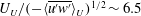 $U_{U}/(-\langle \overline{u^{\prime }w^{\prime }}\rangle _{U})^{1/2}\sim 6.5$
for
$U_{U}/(-\langle \overline{u^{\prime }w^{\prime }}\rangle _{U})^{1/2}\sim 6.5$
for
 $Re_{K}>O(1)$
. This relation is however larger than the 2.6 value suggested in G09.
$Re_{K}>O(1)$
. This relation is however larger than the 2.6 value suggested in G09.
5 Discussion
Our hydrodynamic framework and the use of a novel experimental approach provides a description of the nature of interaction between permeable sediments and the overlying flow. This framework places flow at the SWI in the context of two extreme flow typologies, impermeable boundary layer flow and flow over highly permeable boundaries, through consideration of the dependence of the flow on
 $Re_{K}$
. As typical aquatic sediments correspond to moderate values of
$Re_{K}$
. As typical aquatic sediments correspond to moderate values of
 $Re_{K}$
, elements of the hydrodynamic characteristics of both extremes can be seen in the flow at the SWI. The experimental data describe the flow across the SWI for a broad range of
$Re_{K}$
, elements of the hydrodynamic characteristics of both extremes can be seen in the flow at the SWI. The experimental data describe the flow across the SWI for a broad range of
 $Re_{K}$
relevant to aquatic systems.
$Re_{K}$
relevant to aquatic systems.
The results presented here confirm the strong correlation between interfacial flow properties and the relative permeability, where key properties such as the Brinkman layer thickness, shear stress penetration depth, the interfacial turbulence intensities, turbulent shear stress and mean velocity all increase with
 $Re_{K}$
. Values in the limit of
$Re_{K}$
. Values in the limit of
 $Re_{K}\rightarrow 0$
correspond to values typically expected for impermeable boundary layer flow, with the exception of the interfacial velocity and Brinkman layer thickness, which is argued to be the consequence of a heterogeneous interface region.
$Re_{K}\rightarrow 0$
correspond to values typically expected for impermeable boundary layer flow, with the exception of the interfacial velocity and Brinkman layer thickness, which is argued to be the consequence of a heterogeneous interface region.
At the high
 $Re_{K}$
limit, the properties at the inflection point in the velocity profile are consistent with the relations suggested in G09 for flows over highly permeable boundaries. Our data suggest that all flows at the SWI possess an inflectional velocity profile. An observation consistent with the results of Goharzadeh et al. (Reference Goharzadeh, Khalili and Jørgensen2005) and Breugem et al. (Reference Breugem, Boersma and Uittenbogaard2006), however, inconsistent with the results of Nikora et al. (Reference Nikora, Goring, McEwan and Griffiths2001) and Mignot et al. (Reference Mignot, Barthelemy and Hurther2009). Given that the velocity profile below the interface (i.e. over the Brinkman layer) matches that of a hyperbolic tangent profile, the mean streamwise velocity at and below the interface is consistent with that in flows over a highly permeable boundary.
$Re_{K}$
limit, the properties at the inflection point in the velocity profile are consistent with the relations suggested in G09 for flows over highly permeable boundaries. Our data suggest that all flows at the SWI possess an inflectional velocity profile. An observation consistent with the results of Goharzadeh et al. (Reference Goharzadeh, Khalili and Jørgensen2005) and Breugem et al. (Reference Breugem, Boersma and Uittenbogaard2006), however, inconsistent with the results of Nikora et al. (Reference Nikora, Goring, McEwan and Griffiths2001) and Mignot et al. (Reference Mignot, Barthelemy and Hurther2009). Given that the velocity profile below the interface (i.e. over the Brinkman layer) matches that of a hyperbolic tangent profile, the mean streamwise velocity at and below the interface is consistent with that in flows over a highly permeable boundary.
Flows over sediments are, however, still typically treated as impermeable. While the region around the SWI (
 $z=[-\unicode[STIX]{x1D6FF}_{b},z_{U}]$
) is small compared to the boundary layer thickness, it is exactly this region where the flow and sediment properties influence the interfacial transport processes. Our results suggest that this region invariably shows similarities to that of a highly permeable boundary, with the penetration of momentum across the interface and the presence of an inflectional velocity profile. Beyond
$z=[-\unicode[STIX]{x1D6FF}_{b},z_{U}]$
) is small compared to the boundary layer thickness, it is exactly this region where the flow and sediment properties influence the interfacial transport processes. Our results suggest that this region invariably shows similarities to that of a highly permeable boundary, with the penetration of momentum across the interface and the presence of an inflectional velocity profile. Beyond
 $Re_{K}\sim 1{-}2$
, transition is observed for key interfacial flow characteristics towards the asymptotic limits described for highly permeable boundaries, for instance the penetration of the turbulent shear stress. These similarities with highly permeable boundaries suggest a change in our perspective on flows over porous media; namely for
$Re_{K}\sim 1{-}2$
, transition is observed for key interfacial flow characteristics towards the asymptotic limits described for highly permeable boundaries, for instance the penetration of the turbulent shear stress. These similarities with highly permeable boundaries suggest a change in our perspective on flows over porous media; namely for
 $Re_{K}\rightarrow 0$
the flow closely resembles that over an impermeable boundary, while for increasing
$Re_{K}\rightarrow 0$
the flow closely resembles that over an impermeable boundary, while for increasing
 $Re_{K}$
flow characteristics of the highly permeable boundary become increasingly apparent. More importantly, the conceptual linking between the impermeable boundary and the highly permeable boundary allows for a universal description (based on
$Re_{K}$
flow characteristics of the highly permeable boundary become increasingly apparent. More importantly, the conceptual linking between the impermeable boundary and the highly permeable boundary allows for a universal description (based on
 $Re_{K}$
) of flows over granular beds.
$Re_{K}$
) of flows over granular beds.
These results have implications on the current use of popular interfacial transport models. The DBL model, for instance, assumes sediments to be impenetrable by the flow and cannot describe such features as a non-zero Brinkman layer thickness and a non-zero interfacial velocity. Increasing
 $Re_{K}$
even leads to the penetration of turbulent fluctuations and turbulent shear stress into the sediment, which clearly conflicts with the concept of a diffusive boundary layer above the SWI. While slip models do allow flow penetration, they rely heavily on experimental verification as the models require input of the interfacial velocity, the Brinkman layer thickness and/or the eddy viscosity profile. It has long been argued that
$Re_{K}$
even leads to the penetration of turbulent fluctuations and turbulent shear stress into the sediment, which clearly conflicts with the concept of a diffusive boundary layer above the SWI. While slip models do allow flow penetration, they rely heavily on experimental verification as the models require input of the interfacial velocity, the Brinkman layer thickness and/or the eddy viscosity profile. It has long been argued that
 $\unicode[STIX]{x1D6FF}_{b}\propto \sqrt{K}$
, but this simple scaling is not fully supported by our results. Our results suggest that the performance of the slip model is highly dependent on the closure model used. Even if the Brinkman layer thickness can be reasonably predicted, the slip model needs further input on the contribution of turbulence across the interface, possibly in the form of an eddy viscosity model, to provide accuracy over a wide range of
$\unicode[STIX]{x1D6FF}_{b}\propto \sqrt{K}$
, but this simple scaling is not fully supported by our results. Our results suggest that the performance of the slip model is highly dependent on the closure model used. Even if the Brinkman layer thickness can be reasonably predicted, the slip model needs further input on the contribution of turbulence across the interface, possibly in the form of an eddy viscosity model, to provide accuracy over a wide range of
 $Re_{K}$
.
$Re_{K}$
.
A novel modelling approach based on the
 $Re_{K}$
framework seems a strong alternative given the encouraging correlations between
$Re_{K}$
framework seems a strong alternative given the encouraging correlations between
 $Re_{K}$
and key interfacial transport properties. The continuous variation of these key properties from
$Re_{K}$
and key interfacial transport properties. The continuous variation of these key properties from
 $Re_{K}\ll 1$
to
$Re_{K}\ll 1$
to
 $Re_{K}\gg 1$
, suggests that such a model is potentially much broader in its practical application than the DBL and slip models, while being possibly more simple considering the dependency on a single parameter.
$Re_{K}\gg 1$
, suggests that such a model is potentially much broader in its practical application than the DBL and slip models, while being possibly more simple considering the dependency on a single parameter.
Though the results presented consider momentum transport only, the presence of a turbulent flow field across the interface has implications for the transport of mass. Our results show that turbulent activity, albeit small, is still present at the interface for the lowest value of
 $Re_{K}$
(
$Re_{K}$
(
 $Re_{K}=0.36$
), and this can be significant for scalar transport, with tracer molecular diffusivities of
$Re_{K}=0.36$
), and this can be significant for scalar transport, with tracer molecular diffusivities of
 $O(10^{-9}~\text{m}^{2}~\text{s}^{-1})$
. This is consistent with the data shown in figure 1, where only at
$O(10^{-9}~\text{m}^{2}~\text{s}^{-1})$
. This is consistent with the data shown in figure 1, where only at
 $Re_{K}\sim O(0.01)$
is the eddy diffusivity equal to the molecular diffusivity. It suggests that for
$Re_{K}\sim O(0.01)$
is the eddy diffusivity equal to the molecular diffusivity. It suggests that for
 $Re_{K}>0.1$
turbulent activity is responsible for the enhanced diffusivities shown in figure 1.
$Re_{K}>0.1$
turbulent activity is responsible for the enhanced diffusivities shown in figure 1.
Further research is required on the impact of other sediment bed properties on the interfacial hydrodynamics. In particular, consideration of the length scale of the roughness elements,
 $k_{s}$
, will allow extension of this framework beyond monodisperse granular beds, where
$k_{s}$
, will allow extension of this framework beyond monodisperse granular beds, where
 $k_{s}$
is strongly correlated to
$k_{s}$
is strongly correlated to
 $\sqrt{K}$
. Comparison of the interfacial flow statistics observed here with those of a polydisperse or non-granular sediment bed would therefore be valuable, as the roughness scale could be varied while maintaining a constant permeability. Although this roughness scale is typically small compared to the boundary layer scale, differences in flow properties across this distance can be significant (contrast the left- and right-hand side of figure 13). Nevertheless, even across the roughness, the local flow properties are strongly dependent on the value of
$\sqrt{K}$
. Comparison of the interfacial flow statistics observed here with those of a polydisperse or non-granular sediment bed would therefore be valuable, as the roughness scale could be varied while maintaining a constant permeability. Although this roughness scale is typically small compared to the boundary layer scale, differences in flow properties across this distance can be significant (contrast the left- and right-hand side of figure 13). Nevertheless, even across the roughness, the local flow properties are strongly dependent on the value of
 $Re_{K}$
.
$Re_{K}$
.
6 Conclusions
A basic framework has been proposed describing the hydrodynamics across the sediment–water interface in terms of the permeability Reynolds number,
 $Re_{K}$
. This framework represents a combination of canonical flow typologies, namely impermeable boundary layer flow (
$Re_{K}$
. This framework represents a combination of canonical flow typologies, namely impermeable boundary layer flow (
 $Re_{K}\ll 1$
) and highly permeable canopy flows (
$Re_{K}\ll 1$
) and highly permeable canopy flows (
 $Re_{K}\gg 1$
). As both flow typologies are characterised by distinct features, the framework suggests that flow at the sediment–water interface in aquatic systems (typically at
$Re_{K}\gg 1$
). As both flow typologies are characterised by distinct features, the framework suggests that flow at the sediment–water interface in aquatic systems (typically at
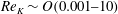 $Re_{K}\sim O(0.001{-}10)$
) represents a mixture of the flow characteristics in either limit.
$Re_{K}\sim O(0.001{-}10)$
) represents a mixture of the flow characteristics in either limit.
This framework is supported by novel experimental results across the SWI, highlighted by the existence of flow and shear stress penetration into the sediment bed and the presence of a velocity inflection point above the SWI. These features and other statistics at the SWI are consistent with the variation of the wall-blocking effect and show a strong correlation with
 $Re_{K}$
. Many of these properties become independent of
$Re_{K}$
. Many of these properties become independent of
 $Re_{K}$
as it increases, tending towards behaviour found in flows over highly permeable boundaries (i.e. canopies). These results suggest that a transition in interfacial flow properties occurs at
$Re_{K}$
as it increases, tending towards behaviour found in flows over highly permeable boundaries (i.e. canopies). These results suggest that a transition in interfacial flow properties occurs at
 $Re_{K}\simeq 1{-}2$
, beyond which the turbulent shear stress starts to dominate the total shear stress at the interface, the turbulent penetration into the sediment becomes comparable to that of the mean flow and the inflectional velocity and turbulence intensities show good agreement with the predictive relations suggested for highly permeable boundaries.
$Re_{K}\simeq 1{-}2$
, beyond which the turbulent shear stress starts to dominate the total shear stress at the interface, the turbulent penetration into the sediment becomes comparable to that of the mean flow and the inflectional velocity and turbulence intensities show good agreement with the predictive relations suggested for highly permeable boundaries.
The explicit findings of turbulence penetration into the sediment bed has major consequences for the application of mass and momentum transport models. The most common, the DBL model, does not account for the penetration of flow across the interface, let alone turbulence, making its application limited to
 $Re_{K}\sim O(0.01)$
. Moreover, models that do account for flow penetration, such as the slip model, are highly sensitive to the definition of the interface and employ boundary conditions that are found to be erroneous here. One such example is the Brinkman layer thickness, whose ratio to
$Re_{K}\sim O(0.01)$
. Moreover, models that do account for flow penetration, such as the slip model, are highly sensitive to the definition of the interface and employ boundary conditions that are found to be erroneous here. One such example is the Brinkman layer thickness, whose ratio to
 $\sqrt{K}$
is often taken to be constant. Here, however, it is shown to exhibit a strong correlation with
$\sqrt{K}$
is often taken to be constant. Here, however, it is shown to exhibit a strong correlation with
 $Re_{K}$
. The results presented here suggest that future predictive models for sediment-bounded flow should be based on this
$Re_{K}$
. The results presented here suggest that future predictive models for sediment-bounded flow should be based on this
 $Re_{K}$
framework, which could condense the wide range of currently employed models that require complex input and calibration.
$Re_{K}$
framework, which could condense the wide range of currently employed models that require complex input and calibration.
Acknowledgements
The authors would like to thank the anonymous reviewers whose insightful comments have helped to improve this manuscript. This research was supported under the Australian Research Council’s Discovery Projects funding scheme (project no. DP120102500).


