


1. Introduction
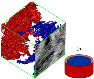
Thermal convection is an important transport mechanism in many engineering and geophysical flows. Centrifugal buoyancy-driven convection (figure 1) is a canonical thermal convection system to study some of these flows (table 1). The studies with geophysical interests consider this system as a closed dynamical model for the earth's liquid (outer) core (Busse & Carrigan Reference Busse and Carrigan1974), or midlatitude atmosphere (Randriamampianina et al. Reference Randriamampianina, Früh, Read and Maubert2006; Read et al. Reference Read, Maubert, Randriamampianina and Früh2008; Von Larcher et al. Reference Von Larcher, Viazzo, Harlander, Vincze and Randriamampianina2018). The studies with turbomachinery interests consider this system as a model for the compressor cavity (Bohn et al. Reference Bohn, Deuker, Emunds and Gorzelitz1995; King, Wilson & Owen Reference King, Wilson and Owen2007; Owen & Long Reference Owen and Long2015; Pitz et al. Reference Pitz, Chew, Marxen and Hills2017a; Pitz, Marxen & Chew Reference Pitz, Marxen and Chew2017b). The system is a rotating cylindrical shell with inner cold wall and outer hot wall (figure 1). Rotation introduces centrifugal buoyancy (set by centripetal acceleration) and Coriolis forces.

Figure 1. Set-up of flow. (a) Centrifugal buoyancy-driven convection in the cylindrical shell with gap  $H$ and outer radius
  $R$. The shell undergoes solid-body clockwise rotation about its axis
  $\zeta$, with rotational speed
  $\varOmega$. The outer wall is hotter than the inner core. (b) Our computational domain as a small chunk of centrifugal convection, highlighted with dashed lines in panel (a), with
  $H \ll R$, which is rectilinear, and
  $L_x$ and
  $L_y$ are the domain sizes in the streamwise (circumferential) and spanwise (axial) directions. Due to thin-shell approximation, the computational domain is exposed to a uniform centripetal acceleration
  $\varOmega ^{2} R \gg g$, so that gravity does not matter here.
Table 1. Schematic representation and previous studies of centrifugal convection and rotating Rayleigh–Bénard convection. We name the systems based on their boundary conditions (wall or slip).
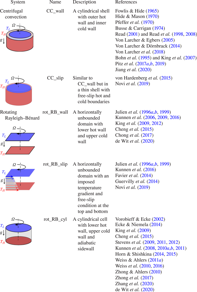
Centrifugal convection differs from rotating Rayleigh–Bénard convection (table 1). In centrifugal convection, the axis of rotation is parallel to the hot and cold walls (normal to the centrifugal buoyancy force), while in rotating Rayleigh–Bénard convection, the axis of rotation is normal to the hot and cold walls (parallel to the gravitational buoyancy force). However, both systems are characterised by the Rayleigh number  $Ra$, inverse Rossby number
  $Ro^{-1}$ and Prandtl number
  $Pr$ (assuming that gravity is neglected in centrifugal convection, figure 1a). In centrifugal convection, these numbers are defined as
 \begin{gather} Ra \equiv (U H)^{2}/(\nu \kappa) = (\varOmega^{2} R \beta \varDelta H^{3})/(\nu \kappa), \end{gather}
 \begin{gather}Ro^{-1} \equiv (2\varOmega H)/U = 2(\beta \varDelta R/H)^{-1/2}, \end{gather}
 \begin{gather}Pr \equiv \nu/\kappa, \end{gather}
where  $U \equiv (\varOmega ^{2} R \beta \varDelta H)^{1/2}$, the free-fall velocity;
  $\varOmega$ is the rotational speed;
  $R$ is the outer shell radius;
  $H$ is the shell thickness;
  $\varDelta \equiv (T_H - T_L)$, the temperature difference;
  $\beta$ is the thermal expansion coefficient;
  $\kappa$ is the thermal diffusivity;
  $\nu$ is the kinematic viscosity. For convenience, we only use the inverse Rossby number
  $Ro^{-1}$ (rather than
  $Ro$), as it is directly linked to the Coriolis force (i.e. higher
  $Ro^{-1}$ implies higher Coriolis force).
In figure 2, we compile a  $(Ra,Ro^{-1})$ parameter space of the previous studies on centrifugal convection (figure 2a) and rotating Rayleigh–Bénard convection (figure 2b). We list these studies in table 1. We also add two recent sets of data points for centrifugal convection (figure 2a). One is our present data (
 $\circ$, black) and the other one is by our coauthor, Professor C. Sun and his colleagues (
 $\diamondsuit$, dark grey
  $\diamondsuit$, process blue
  $\diamondsuit$, dark orange; Jiang et al. (Reference Jiang, Zhu, Wang, Huisman and Sun2020)). This figure highlights the importance of studying centrifugal convection, as a system that is explored to a lesser extent than rotating Rayleigh–Bénard convection. Rotating Rayleigh–Bénard convection has been investigated over almost a continuous parameter sweep of
  $10^{4} \lesssim Ra \lesssim 10^{15}$ and
  $0 \lesssim Ro^{-1} \lesssim 100$. However, until recent studies (
 $\circ$, black;
  $\diamondsuit$, dark grey;
  $\diamondsuit$, process blue;
  $\diamondsuit$, dark orange), centrifugal convection was investigated at limited values of
  $Ra$ and
  $Ro^{-1}$, and only for
  $Ro^{-1} \gtrsim 2$ (large Coriolis force). von Hardenberg et al. (Reference von Hardenberg, Goluskin, Provenzale and Spiegel2015) study
  $Ro^{-1}<2$ (
 $\triangledown$, red), but they consider
  $Ra = 10^{7}$. Also, their set-up is free-slip hot and cold plates rotating about a distant axis. This set-up can be perceived as a slice of a thin cylindrical shell with free-slip boundaries (CC_slip in table 1). The previous studies focus on large
  $Ro^{-1}$ because experiments are constrained by their working fluid and apparatus, and numerical studies set their parameter space following the experiments. For instance, among the geophysical studies, Read et al. (Reference Read, Maubert, Randriamampianina and Früh2008) (
 $\triangle$, blue) follow the experiment of Fowlis & Hide (Reference Fowlis and Hide1965), and Von Larcher et al. (Reference Von Larcher, Viazzo, Harlander, Vincze and Randriamampianina2018) (
 $\triangle$, black) follow their own experiment. Among the turbomachinery studies, Pitz et al. (Reference Pitz, Chew, Marxen and Hills2017a,Reference Pitz, Marxen and Chewb) (
 $\square$, red) and King et al. (Reference King, Wilson and Owen2007) (
 $\square$, black) follow the experiment of Bohn et al. (Reference Bohn, Deuker, Emunds and Gorzelitz1995) (
 $\square$, blue).

Figure 2. Parameter space of  $Ra$ and
  $Ro^{-1}$ corresponding to our present simulations (
 $\circ$, black in panel a) and the previous studies listed in table 1 for (a) centrifugal convection (shaded regions or open symbols) and (b) rotating Rayleigh–Bénard convection (filled symbols). For centrifugal convection, the data of Jiang et al. (Reference Jiang, Zhu, Wang, Huisman and Sun2020) are divided between three-dimensional direct numerical simulations (DNS) (
 $\diamondsuit$, dark grey), two-dimensional DNS (
 $\diamondsuit$, process blue) and experiments (
 $\diamondsuit$, dark orange). Shaded regions or open triangles correspond to the studies with geophysical interests, and open squares correspond to the studies with turbomachinery interests. The shaded regions highlight the approximate parameter space, because the exact (
 $Ro^{-1},Ra$) values are not reported. For rotating Rayleigh–Bénard convection, the symbol shape is different between rot_RB_wall (filled triangle), rot_RB_slip (filled square) and rot_RB_cyl (filled circle). For centrifugal convection,
  $Ra$ and
  $Ro^{-1}$ are defined based on (1.1a) and (1.1b), respectively, where for the studies with finite shell thickness we pick
  $R$ as the average of inner core and outer wall radius. For rotating Rayleigh–Bénard convection,
  $Ra \equiv \beta g \varDelta H^{3}/(\kappa \nu )$ and
  $Ro^{-1} \equiv 2\varOmega (g \beta \varDelta /H )^{-1/2}$, where
  $g$ is gravity and
  $\beta , \varDelta , \varOmega , \nu , \kappa$ are the same as those in (1.1a)–(1.1c) and
  $H$ is the height of the sample between the top (cold) wall and bottom (hot) wall.
Here, we perform DNS at  $Ra = (10^{7}, 10^{8}, 10^{9}, 10^{10})$ and
  $Ro^{-1} = (0, 0.3, 0.5, 0.6, 0.8, 1.0)$, (
 $\circ$, black in figure 2a). Additionally, we explore
  $(Ra,Ro^{-1}) = (10^{7},2.0)$ and
  $(Ra,Ro^{-1}) = (10^{8},20.0)$ that fall into the regimes of interest by the geophysical and turbomachinery studies. Our objectives are to investigate: (i) the flow regimes from no Coriolis force (
 $Ro^{-1} = 0$) to a very large Coriolis force (
 $Ro^{-1} = 20$); (ii) the universality of these regimes from
  $Ra = 10^{7}$ to
  $10^{10}$; and (iii) the analogy between these regimes and those in rotating Rayleigh–Bénard convection. We show how an optimal choice of
  $Ro^{-1}$ can exploit the Coriolis force to tune a persistent large-scale wind. On the other hand, we show how large
  $Ro^{-1}\ge 1$ can cause the Coriolis force to suppress turbulence and laminarise the flow. The organised wind is a feature of this system. It hastens the boundary layer transition from laminar to turbulent, i.e. transition from the classical regime (Grossmann & Lohse Reference Grossmann and Lohse2000) to the ultimate regime (Grossmann & Lohse Reference Grossmann and Lohse2011). In the classical regime, the effective heat-transfer scaling, expressed through an effective power law for the Nusselt number
  $Nu$ to
  $Ra$ relationship (
 $Nu \propto Ra^{\alpha }$), follows an effective power-law exponent
  $\alpha \le 1/3$ (Grossmann & Lohse Reference Grossmann and Lohse2000). However, in the ultimate regime the heat-transfer scaling follows a steeper gradient with an effective exponent
  $\alpha > 1/3$ (Grossmann & Lohse Reference Grossmann and Lohse2011).
The ultimate regime has been approached or fully reached in several turbulent systems, including Rayleigh–Bénard convection (Roche et al. Reference Roche, Gauthier, Chabaud and Hébral2005; Ahlers et al. Reference Ahlers, He, Funfschilling and Bodenschatz2012; He et al. Reference He, Funfschilling, Bodenschatz and Ahlers2012a,Reference He, Funfschilling, Nobach, Bodenschatz and Ahlersb, Reference He, Funfschilling, Nobach, Bodenschatz and Ahlers2013; He, Bodenschatz & Ahlers Reference He, Bodenschatz and Ahlers2016), the analogue Taylor–Couette flow (see the review by Grossmann, Lohse & Sun (Reference Grossmann, Lohse and Sun2016)), and vertical natural convection (Ng et al. Reference Ng, Ooi, Lohse and Chung2017) or sheared convection (Pirozzoli et al. (Reference Pirozzoli, Bernardini, Verzicco and Orlandi2017) and Blass et al. (Reference Blass, Zhu, Verzicco, Lohse and Stevens2020), though by far not reached here). The three latter systems benefit from a persistent wind, similar to centrifugal convection. However, the source of wind formation, i.e. shear, differs among these systems; in Taylor–Couette flow the shear is due to differentially rotating cylinders, in sheared convection the shear is due to differentially moving walls, in vertical convection the shear is due to gravitational buoyancy, and in centrifugal convection the shear is due to the Coriolis force. Centrifugal convection is unique among these systems, because the wind forms due to the Coriolis force that does not alter the kinetic energy. Our coauthor, Professor C. Sun, has proposed this system as an ideal opportunity to reach the ultimate turbulent regime, to mitigate possible non-Oberbeck–Boussinesq effects at large  $Ra$ in the standard Rayleigh–Bénard geometry, as here the possible ultimate regime is now triggered by centrifugal buoyancy instead of by temperature differences. It was this proposition which triggered the present numerical work.
The paper is organised as follows. In § 2 we describe our DNS set-up as well as simulation and grid convergence studies. In the results section (§ 3), first, we identify the overall flow regimes (§ 3.1) through flow visualisation,  $Nu$ and skin-friction coefficient
  $C_f$. Then, we discuss each flow regime from the bidirectional wind formation (§ 3.2) to the flow laminarisation (§ 3.5). In § 3.6 we show the onset of transition to turbulent by the bidirectional wind. The concluding remarks follow in § 4.
2. Flow set-up
2.1. Governing equations
The governing equations are derived from the incompressible Navier–Stokes equations governing the flow in a concentric cylindrical annulus with gap  $H$ (figure 1a) in the frame rotating in a clockwise direction about its cylindrical axis
  $\zeta$ at constant rotational speed
  $\varOmega$, as described by velocity
  $\boldsymbol {v} = v_r \boldsymbol {e}_r + v_{\phi } \boldsymbol {e}_{\phi } + v_{\zeta } \boldsymbol {e}_{\zeta }$ and temperature
  $T$ in cylindrical coordinates (
 $r,\phi ,\zeta$). The boundary conditions in this rotating frame are no-slip and impermeable walls,
  $\boldsymbol {v}(r = R - H) =\boldsymbol {v}(r = R) = 0$, corresponding to the inner core and outer wall, respectively, and isothermal walls with the prescribed temperature difference
  $\varDelta = T_H - T_L$, with
  $T(r = R - H) = T_L$ and
  $T(r = R) = T_H$, corresponding to an inner colder core and an outer hotter wall. We have invoked the Oberbeck–Boussinesq approximation, which assumes constant fluid properties,
  $\nu$,
  $\kappa$ and
  $\beta$, and that density variations are only dynamically important in the buoyancy term. In the buoyancy term the density variation is
  $(\rho - \rho _o) = -\beta \rho _o \theta$, where
  $\rho _o = \rho (T_o=(T_H+T_L)/2)$, the reference density at temperature
  $T_o$, and
  $\theta = T-T_o$, the temperature variation relative to
  $T_o$. For the sake of brevity we refer the reader to Kundu & Cohen (Reference Kundu and Cohen1990), for example, for the equations in the
  $(r,\phi ,\zeta )$ coordinate system. Since the equations are presented in a rotating frame, two additional terms appear in the Navier–Stokes equations: the Coriolis force,
  $-2\varOmega v_{\phi } \boldsymbol {e}_r+2\varOmega v_r \boldsymbol {e}_{\phi }$, and the centripetal acceleration,
  $-\beta \varOmega ^{2} r \theta \boldsymbol {e}_r$.
To further simplify the problem, we consider the thin-shell (unity radius ratio) limit,  $\epsilon \equiv H/R \ll 1$ (figure 1b). To this end, we transform the equations from
  $(r,\phi ,\zeta )$ into curvilinear coordinates
  $(x, y, z)$ with the origin placed at the outer cylinder. The transformed coordinates will be
  $x = r \phi , y=-\zeta , z = R-r$, and the transformed velocity will be
  $u = v_{\phi }, v = -v_{\zeta }, w = -v_r$. Then, we non-dimensionalise the variables using the gap width
  $H$, the free-fall velocity
  $U \equiv (\varOmega ^{2} R \beta \varDelta H)^{1/2}$, and
  $\varDelta$:
  $\tilde {x} = x/H$,
  $\tilde {y} = y/H$,
  $\tilde {z} = z/H$,
  $\tilde {t} = tU/H$ are the scaled space and time coordinates;
  $\tilde {u} = u/U$,
  $\tilde {v} = v/U$,
  $\tilde {w} = w/U$ are the scaled velocity components; and
  $\tilde {p} = (p-\rho _o \varOmega ^{2} R^{2}/2)/(\rho _o U^{2})$ and
  $\tilde {\theta } = \theta /\varDelta$ are the scaled pressure and temperature variation. Substituting these into the transformed equation, and expanding in small
  $\epsilon$, we obtain, to leading order
 \begin{gather} \tilde{\boldsymbol{\nabla}}\boldsymbol{\cdot}\tilde{\boldsymbol{u}}= 0, \end{gather}
 \begin{gather}\partial_{\tilde{t}} \tilde{u} +\tilde{\boldsymbol{u}}\boldsymbol{\cdot}\tilde{\boldsymbol{\nabla}}\tilde{u}= -\partial_{\tilde{x}} \tilde{p} +(Ra/Pr)^{-1/2}\tilde{\nabla}^{2} \tilde{u} -Ro^{-1} \tilde{w}, \end{gather}
 \begin{gather}\partial_{\tilde{t}} \tilde{v} +\tilde{\boldsymbol{u}}\boldsymbol{\cdot}\tilde{\boldsymbol{\nabla}}\tilde{v} = -\partial_{\tilde{y}} \tilde{p} +(Ra/Pr)^{-1/2}\tilde{\nabla}^{2} \tilde{v},\end{gather}
 \begin{gather}\partial_{\tilde{t}} \tilde{w} +\tilde{\boldsymbol{u}}\boldsymbol{\cdot}\tilde{\boldsymbol{\nabla}}\tilde{w} = -\partial_{\tilde{z}} \tilde{p} +(Ra/Pr)^{-1/2}\tilde{\nabla}^{2} \tilde{w} +Ro^{-1} \tilde{u}+\tilde{\theta}, \end{gather}
 \begin{gather}\partial_{\tilde{t}} \tilde{\theta} +\tilde{\boldsymbol{u}}\boldsymbol{\cdot}\tilde{\boldsymbol{\nabla}}\tilde{\theta} = (Ra\,Pr)^{-1/2}\tilde{\nabla}^{2}\tilde{\theta}. \end{gather}
In (2.1a)–(2.1e), the Rayleigh number  $Ra$, the inverse Rossby number
  $Ro^{-1}$ and the Prandtl number
  $Pr$, as introduced in (1.1a)–(1.1c), are the control parameters. Since
  $\tilde {x} = O(1)$ and
  $\tilde {y} = O(1)$, the thin-shell limit implies
  $x \ll R$ and
  $y \ll R$, i.e. the computational domain is a small chunk of the concentric cylinder (indicated with dashed lines in figure 1a). Therefore, the transformed (2.1a)–(2.1e) that are identical to the Navier–Stokes equations in the Cartesian coordinate system are solved in a rectilinear box (figure 1b). The transformed boundary conditions in the
  $x$- and
  $y$-directions are periodic and at the outer and inner walls are
  $\tilde {\boldsymbol {u}}(\tilde {z} = 0) = \tilde {\boldsymbol {u}}(\tilde {z} = 1) = 0$,
  $\tilde {\theta }(\tilde {z} = 0) = 1/2$ and
  $\tilde {\theta }(\tilde {z} = 1) = -1/2$.
The results are presented in terms of  $(x,u)$,
  $(z,w)$ and
  $(y,v)$, the circumferential, (negative) radial and (negative) axial directions of the cylindrical shell, respectively, and are noted as the streamwise, wall-normal and spanwise directions. The inner and outer walls of the cylindrical shell are also noted as the top and bottom walls, respectively. In the entire manuscript, we denote a non-dimensionalised quantity by
  $U$ and
  $H$ with tilde (e.g.
  $\tilde {t} = tU/H$), an
  $xy$-plane and time averaged quantity with overbar (e.g.
  $\bar {u}$), a volume and time averaged quantity with angle bracket (e.g.
  $\left \langle u \right \rangle$) and an averaged quantity over a specific direction with superscript (e.g.
  $u^{y}$ is averaged in the
  $y$-direction). Fluctuating quantities are obtained by subtracting
  $xy$-plane and time averaged quantities from their instantaneous counterpart (e.g.
  $u'= u - \bar {u}$).
2.2. DNS
The equations are solved using a fully conservative fourth-order finite-difference code, validated in the previous DNS studies of similar flow physics (Ng et al. Reference Ng, Ooi, Lohse and Chung2015, Reference Ng, Ooi, Lohse and Chung2017, Reference Ng, Ooi, Lohse and Chung2018). Table 2 lists all the simulation cases and figure 3 shows the visualizations of the production runs. For all cases,  $Pr=0.7$ and
  $L_x/H \times L_y / H = 1 \times 1$. We choose a fixed aspect ratio of
  $\varGamma = 1$ to focus on the Coriolis force effect (
 $Ro^{-1}$) and achieve the highest possible
  $Ra$. Nevertheless, we speculate that the essential physics, hence the trend in
  $Nu$ and skin-friction coefficient
  $C_f$ do not change with
  $\varGamma$. Our conjecture is based on the previous studies on centrifugal convection and similar thermal convection systems. In classical Rayleigh–Bénard convection, the sensitivity of
  $Nu$ with
  $\varGamma \ge 1$ is less than
  $7\,\%$ for
  $Ra \gtrsim 2 \times 10^{7}$ (figure 4a in Stevens et al. (Reference Stevens, Blass, Zhu, Verzicco and Lohse2018)). The sensitivity of
  $\alpha$ (
 $Nu \propto Ra^{\alpha }$) with
  $\varGamma \ge 1$ is less than
  $3\,\%$ for
  $Ra \gtrsim 10^{9}$ (we analysed figure 3 of Zhou et al. (Reference Zhou, Liu, Li and Zhong2012)). In rotating Rayleigh–Bénard convection,
  $Nu$ is almost insensitive to
  $\varGamma \ge 1$ for
  $Ro^{-1} \ge 0.4$ (figure 4 in Stevens et al. (Reference Stevens, Overkamp, Lohse and Clercx2011)). Even for
  $Ro^{-1} < 0.4$,
  $Nu$ versus
  $Ro^{-1}$ shows the same trend for different
  $\varGamma$. In centrifugal convection, the trend in
  $Nu$ versus
  $Ro^{-1}$ for a full cylindrical shell (figure 2a in Jiang et al. (Reference Jiang, Zhu, Wang, Huisman and Sun2020)) is similar to what we report in § 3.1. Also, the flow regimes that we discuss in § 3 are similar to the previous experiments. At low rotational speed, experiments report an axisymmetric flow, circulating parallel to the walls (e.g. figure 2a,b in Fowlis & Hide (Reference Fowlis and Hide1965); figure 13e,f in Hide & Mason (Reference Hide and Mason1970)). We observe similar flow regime (bidirectional wind) in § 3.2. At high rotational speed, experiments report geostrophic regime with large-scale quasi-two-dimensional cyclones and anticyclones (e.g. figure 2d–h in Fowlis & Hide (Reference Fowlis and Hide1965); figure 4 in Jiang et al. (Reference Jiang, Zhu, Wang, Huisman and Sun2020)). We observe similar flow regime in § 3.5.
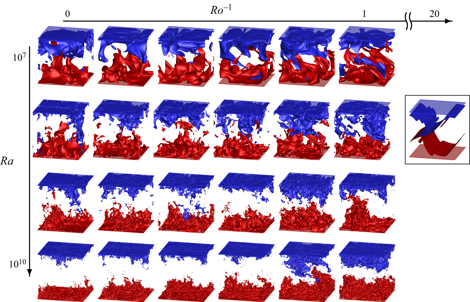
Figure 3. Flow visualisation of the simulation cases. The unframed cases correspond to four Rayleigh numbers  $Ra = (10^{7}, 10^{8}, 10^{9}, 10^{10})$, from the first to the last row, respectively, and six inverse Rossby numbers
  $Ro^{-1} = (0, 0.3, 0.5, 0.6, 0.8, 1.0)$, from the first to the last column, respectively. The special framed case is at
  $Ra= 10^{8}, Ro^{-1} = 20.0$. Isosurface of
  $\theta = -\varDelta /10$ (blue) and
  $\theta = +\varDelta /10$ (red).
Table 2. Simulation parameters and global quantities for parameter and grid-convergence study. The number of grid points  $N$ is the same in all the three directions. Here
  $\tilde {\tau }_{avg} = \tau _{avg}U/H$ is the averaging time period;
  $Nu \equiv (H/\varDelta )|\textrm {d}{\bar {\theta }/\textrm {d}z}|_{w}$ is the Nusselt number, where
  $|\textrm {d}{\bar {\theta }/\textrm {d}z}|_w$ is the absolute wall temperature gradient, averaged over time,
  $xy$-plane and both walls;
  $Nu_h$ is the counterpart of
  $Nu$, averaged over the second half of
  $\tilde {\tau }_{avg}$;
  $Nu_{bot} \equiv (H/\varDelta )|\textrm {d}{\bar {\theta }/\textrm {d} z}|_{z=0}$ is the Nusselt number at the bottom wall averaged over
  $\tilde {\tau }_{avg}$;
  $Diff_{\tau _{avg}} \equiv (Nu-Nu_h)/Nu$;
  $N_{BL}$ is the number of grid points within the thermal boundary layer located by the outer peak of root mean square (r.m.s.) of temperature fluctuation;
  $h = \max (\varDelta _x,\varDelta _y,\varDelta _z)$ is the maximum local grid size, and
  $\eta _l(z) \equiv ( \nu ^{3}/\overline {\varepsilon _u} )^{1/4}$ and
  $\eta _g \equiv ( \nu ^{3}/\left \langle \varepsilon _u \right \rangle )^{1/4}$ are the local and global Kolmogorov length scales;
  $\left \langle \varepsilon _u \right \rangle _{nrm} = \left \langle \varepsilon _u \right \rangle Pr^{2} H^{4} /[ \nu ^{3} (Nu- 1 ) Ra ]$ and
  $\left \langle \varepsilon _{\theta } \right \rangle _{nrm} = \left \langle \varepsilon _{\theta } \right \rangle H^{2}/( \kappa \varDelta ^{2} Nu )$ measure the global balance between the dissipation rates and Nusselt number, a measure of resolution sufficiency (Calzavarini et al. Reference Calzavarini, Lohse, Toschi and Tripiccione2005; Stevens, Verzicco & Lohse Reference Stevens, Verzicco and Lohse2010). For a perfect resolution, the criterion
  $\left \langle \varepsilon _u \right \rangle _{nrm}=\left \langle \varepsilon _{\theta } \right \rangle _{nrm}=1$ must be nearly satisfied, regardless of the scheme used to compute
  $\varepsilon _u$ and
  $\varepsilon _{\theta }$. See the text for discussion.

We use the same number of grid points  $N$ in each direction. The grid points are uniformly distributed in the
  $x$- and
  $y$-directions, and are stretched in the
  $z$-direction. The choice for
  $N$ and stretching factor are decided a priori based on Shishkina et al. (Reference Shishkina, Stevens, Grossmann and Lohse2010, (36), (42) and (43)) to resolve the Kolmogorov scale both in the bulk and within the boundary layers. In table 2, we call these resolutions standard, as we show here that they are suitable for well-resolved DNS. We also performed calculations at coarser and finer resolutions, and we call them coarse and fine, respectively. In total, four values of
  $Ra$ are simulated, ranging from
  $10^{7}$ to
  $10^{10}$, and at each
  $Ra$,
$Ra$,  $Ro^{-1}$ is varied from zero (no Coriolis force) to unity (large Coriolis force). We performed two additional cases: one at
  $Ro^{-1} = 2.0$ for
  $Ra = 10^{7}$, and the other one at
  $Ro^{-1} = 20$ for
  $Ra=10^{8}$, where the Coriolis force is much larger than inertia. We perform an extensive parameter and grid-convergence study (table 2), following the prescriptions by Stevens et al. (Reference Stevens, Verzicco and Lohse2010). For simulation convergence, each case is run for approximately 100 turnover times
  $H/U$ to discard initial transients, and data is averaged over an additional
  $\tau _{avg} \gtrsim 150H/U$ for statistical convergence. Statistical convergence is evaluated based on the Nusselt number
  $Nu \equiv (H/\varDelta )|\textrm {d}{\bar {\theta }/\textrm {d}z}|_{w}$, where
  $|\textrm {d}{\bar {\theta }/\textrm {d}z}|_w = ( |\textrm {d}{\bar {\theta }/\textrm {d}z}|_{z=0} + |\textrm {d}{\bar {\theta }/\textrm {d}z}|_{z=H} )/2$ is the absolute wall temperature gradient, averaged over time,
  $xy$-plane and both walls. We call a simulation statistically converged, once the difference between
  $Nu$ obtained from averaging over
  $\tilde {\tau }_{avg}$ and its counterpart
  $Nu_h$ obtained from averaging over the second half of
  $\tilde {\tau }_{avg}$ is less than
  $1\,\%$ (see
  $Diff_{\tau _{avg}}$ in table 2). We can also see the statistical convergence in the less than
  $1\,\%$ difference between
  $Nu$ and its counterpart at the bottom wall
  $Nu_{bot}$. Another way for statistical convergence is when the difference between top and bottom wall Nusselt numbers
  $Diff_{Nu} = | Nu_{top} - Nu_{bot} |/Nu$ is negligibly small (Kunnen et al. Reference Kunnen, Ostilla-Mónico, van der Poel, Verzicco and Lohse2016). For all cases up to
  $Ra = 10^{9}$,
  $Diff_{Nu}$ is less than
  $2\,\%$.
We perform such an extensive statistical convergence study up to  $Ra = 10^{9}$, where the resolution requirement (maximum
  $N=512$) is affordable to run the calculations for at least
  $250H/U$. The cases at
  $Ra = 10^{10}$ require
  $N= 1024$ for well-resolved simulation, and are substantially expensive. For example, running each well-resolved case at
  $Ra=10^{9}$ (
 $N=512$) for
  $250H/U$, demands approximately
  $0.05$ million central processing unit (CPU) core hours, whereas running each well-resolved case at
  $Ra=10^{10}$ (
 $N=1024$) for
  $250H/U$, demands approximately
  $2.0$ million CPU core hours,
  $40$ times more expensive than
  $Ra=10^{9}$. Given the expensive cost at
  $Ra= 10^{10}$, each case is simulated for at least
  $60H/U$ and statistical averaging is performed over
  $\tau _{avg} \gtrsim 30H/U$. Running these cases to full statistical convergence does not add to the conclusions that we draw by studying the cases up to
  $Ra=10^{9}$. Our primary aim by reporting
  $Ra=10^{10}$ is to demonstrate some evidence of boundary layer transition to turbulent, owing to the favourable role of the Coriolis force.
Grid convergence was evaluated based on three criteria. (i) Resolving the local Kolmogorov scale  $\eta _l(z) \equiv ( \nu ^{3}/\overline {\varepsilon _u} )^{1/4}$, where
  $\varepsilon _u = \nu (\partial u_i/\partial x_j)^{2}$ is the kinetic energy dissipation rate. (ii) Satisfying the global exact relations
  $\left \langle \varepsilon _u \right \rangle = \nu ^{3} (Nu- 1 ) Ra Pr^{-2}/H^{4}$ and
  $\left \langle \varepsilon _{\theta } \right \rangle = \kappa \varDelta ^{2} Nu/H^{2}$, where
  $\varepsilon _{\theta } = \kappa (\partial \theta /\partial x_j )^{2}$ is the thermal energy dissipation rate. (iii) Comparison of parameters of interest between sequentially finer grid resolutions.
Criterion (i) was initially prescribed by Grötzbach (Reference Grötzbach1983), suggesting  $h \le {\rm \pi}\eta _g$, where
  $h = ( \varDelta _x \varDelta _y \varDelta _z )^{1/3}$ is the grid size and
  $\eta _g \equiv ( \nu ^{3}/\left \langle \varepsilon _u \right \rangle )^{1/4}$ is the global Kolmogorov scale, based on the volume and time-averaged dissipation rate. Grötzbach (Reference Grötzbach1983) ignored the anisotropy in the grid (by using the geometric mean for
  $h$) and heterogeneity in the dissipation rate (by integrating
  $\varepsilon _u$ over the domain and time). Stevens et al. (Reference Stevens, Verzicco and Lohse2010) showed that for well-resolved simulations, the anisotropic grid and flow heterogeneity must be taken into account. Therefore, following Stevens et al. (Reference Stevens, Verzicco and Lohse2010) we chose
  $h = \max (\varDelta _x,\varDelta _y,\varDelta _z)$, and calculated the local Kolmogorov scale
  $\eta _l$ in each height based on
  $\overline {\varepsilon _u}$. Also we calculated the global Kolmogorov scale
  $\eta _g$, and in table 2 we compare the maximum ratios
  $( h/\eta _g )_{max}$ and
  $( h/\eta _l )_{max}$. As observed, resolving
  $\eta _l$ demands finer resolution than resolving
  $\eta _g$. Results of Stevens et al. (Reference Stevens, Verzicco and Lohse2010) and our results in table 2 show that the criterion
  $( h/\eta _g )_{max} \le {\rm \pi}$ is not sufficient for well-resolved simulation. For instance, the simulations at
  $Ra=10^{9}$ with
  $N^{3} = 256^{3}$, satisfy
  $( h/\eta _g )_{max}\le {\rm \pi}$ but not
  $( h/\eta _l )_{max} \le {\rm \pi}$, and they poorly satisfy the global exact relations for criterion (ii) (
 $\left \langle \varepsilon _u \right \rangle _{nrm} \simeq \left \langle \varepsilon _{\theta } \right \rangle _{nrm} \simeq 0.90$). For a perfect resolution, the criterion
  $\left \langle \varepsilon _u \right \rangle _{nrm} = \left \langle \varepsilon _{\theta } \right \rangle _{nrm} = 1.0$ must be nearly satisfied, even if
  $\varepsilon _u$ and
  $\varepsilon _{\theta }$ are calculated with a different scheme than the code discretisation scheme. Here, we use a fourth-order kinetic energy conservative and a third-order scalar variance non-conservative code. We compute
  $\varepsilon _u$ and
  $\varepsilon _{\theta }$ using a second-order central differencing scheme. We obtain
  $\left \langle \varepsilon _u \right \rangle _{nrm} \simeq \left \langle \varepsilon _{\theta } \right \rangle _{nrm} \simeq 0.97$, for all the standard resolution cases, similar to Stevens et al. (Reference Stevens, Verzicco and Lohse2010). These standard resolution cases also satisfy criterion (i), i.e.
  $( h/\eta _l )_{max} \le {\rm \pi}$.
In figure 4, we show the adequacy of standard resolution based on criterion (iii). We consider  $Ra = 10^{9}$ and
  $Ro^{-1}=0.8$, comparing
  $\overline {\varepsilon _u}$ and
  $\overline {\varepsilon _{\theta }}$ between three grid resolutions:
  $N = 256$ (coarse),
  $512$ (standard) and
  $1024$ (fine). At the coarse resolution (
 $N= 256$), these quantities are slightly lower than the ones at the standard and fine resolutions (consider the insets in figure 4). However, the difference between the standard and fine resolutions is negligible. According to Stevens et al. (Reference Stevens, Verzicco and Lohse2010), in the under-resolved simulations the gradients are smeared out, and
  $\varepsilon _u$ and
  $\varepsilon _{\theta }$ are underestimated. The results that we present in the rest of this paper (figure 3), correspond to the well-resolved standard resolution cases (table 2).

Figure 4. Comparison of (a) kinetic energy dissipation rate  $\overline {\varepsilon _u}$ and (b) thermal energy dissipation rate
  $\overline {\varepsilon _{\theta }}$, averaged over
  $xy$-plane and time, at
  $Ra=10^{9}$ and
  $Ro^{-1}=0.8$ between three grid resolutions
  $N$: coarse
  $256$ (dashed-dotted blue line), standard
  $512$ (dashed red line) and fine
  $1024$ (solid black line). The insets show the framed areas.
3. Results
3.1. Effect of the Coriolis force on heat and momentum fluxes
The resulting Nusselt number  $Nu = (H/\varDelta )|\textrm {d}{\bar {\theta }/\textrm {d}z}|_{w}$ for all cases is compiled in figure 5. When
  $Ro^{-1} = 0$ (
 $\times$, no Coriolis force),
  $Nu$ is close to the Grossmann & Lohse (Reference Grossmann and Lohse2000) theory (dashed black line), as expected. At each
  $Ra$, as
  $Ro^{-1}$ increases (i.e. Coriolis force increases),
  $Nu$ decreases until it reaches a minimum at an optimal
  $Ro^{-1}_{opt}$; beyond
  $Ro^{-1}_{opt}$,
  $Nu$ increases. This is better shown in figure 6(a), plotting
  $Nu$ versus
  $Ro^{-1}$, at each
  $Ra$. Additionally, in figure 6(b) we plot the skin-friction coefficient
  $C_f = 2 \nu |\textrm {d}{\bar {u}/\textrm {d}z}|_w/U^{2}$ versus
  $Ro^{-1}$, at each
  $Ra$. Here
  $|\textrm {d}{\bar {u}/\textrm {d}z}|_w$ is the modulus of the wall velocity gradient, averaged over time,
  $xy$-plane and both walls. Similar to
  $Nu$, at each
  $Ra$ there is an optimal
  $Ro^{-1}_{opt}$ at which
  $C_f$ becomes maximal. Comparing figure 6(a) with 6(b), the values of
  $Ro^{-1}_{opt}$ for the minimum in
  $Nu$ and the maximum in
  $C_f$ are close to each other, hence minimal heat flux coincides with maximal skin friction. Here
  $Ro^{-1}_{opt}$ depends on
  $Ra$, decreasing from approximately
  $1.0$ at
  $Ra = 10^{7}$, to approximately
  $0.6$ at
  $Ra = 10^{10}$.
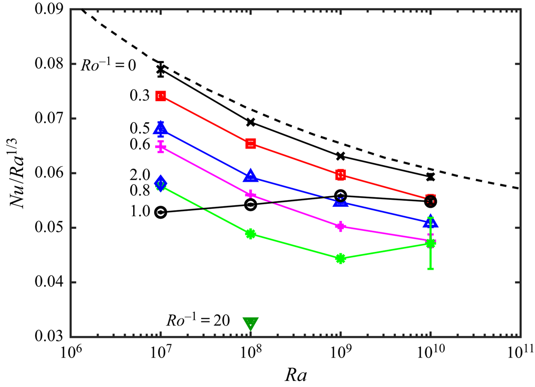
Figure 5. Here  $Nu/Ra^{1/3}$ for all the standard-resolution cases listed in table 2. Here
  $Nu = (H/\varDelta )|\textrm {d}{\bar {\theta }/\textrm {d}z}|_{w}$, where
  $|\textrm {d}{\bar {\theta }/\textrm {d}z}|_w = ( |\textrm {d}{\bar {\theta }/\textrm {d}z}|_{z=0} + |\textrm {d}{\bar {\theta }/\textrm {d}z}|_{z=H} )/2$;
  $Ro^{-1}=0$ (
 $\times$, black),
  $0.3$ (
 $\square$, red),
  $0.5$ (
 $\triangle$, blue),
  $0.6$ (+, magenta),
  $0.8$ (*, green),
  $1.0$ (
 $\circ$, black),
  $2.0$ (
 $\diamond$, blue) and
  $20.0$ (
 $\triangledown$, olive green). Grossmann & Lohse (Reference Grossmann and Lohse2000) theory with the parameters as fixed in Stevens et al. (Reference Stevens, van der Poel, Grossmann and Lohse2013b) (dashed black line). If the error bar
  $| Nu_{top} - Nu_{bot} |/Ra^{1/3}$ is not visible, it is smaller than the symbol size.
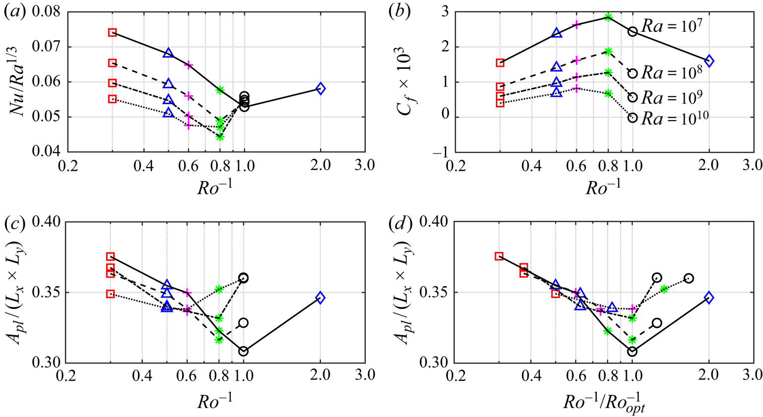
Figure 6. Variation of (a)  $Nu/Ra^{1/3}$, (b)
  $C_f$ and (c,d)
  $A_{pl}$ cold plume coverage at the edge of the bottom wall thermal boundary layer, versus
  $Ro^{-1}$ at different
  $Ra$. Panel (d) is the same as panel (c) except
  $Ro^{-1}$ is scaled by
  $Ro^{-1}_{opt}$, the value of
  $Ro^{-1}$ at minimum
  $A_{pl}$. Here
  $C_f = 2 \nu |\textrm {d}{\bar {u}/\textrm {d}z}|_w/U^{2}$, where
  $|\textrm {d}{\bar {u}/\textrm {d}z}|_w = ( |\textrm {d}{\bar {u}/\textrm {d}z}|_{z=0} + |\textrm {d}{\bar {u}/\textrm {d}z}|_{z=H} )/2$;
  $Ra=10^{7}$ (solid black line),
  $10^{8}$ (dashed black line),
  $10^{9}$ (dashed-dotted black line) and
  $10^{10}$ (dotted black line). Each symbol corresponds to one
  $Ro^{-1}$ consistent with figure 5. Note that in panel (b) at
  $Ra=10^{10}$ and
  $Ro^{-1} = 1.0$ (
 $\circ$, black),
  $C_f \simeq 2 \times 10^{-5}$ (
 $\simeq 0$ on the given linear scale for
  $C_f$), where the flow is at the onset of reversal.
To explain the underlying mechanism for the behaviour seen in  $Nu$ and
  $C_f$ versus
  $Ro^{-1}$, we study the flow at different values of
  $Ro^{-1}$ (figure 7). We focus on
  $Ra=10^{8}$, but our conclusions can be generalised to other values of
  $Ra$. In figure 7(e–h), we show the instantaneous spanwise averaged temperature field
  $\theta ^{y}/\varDelta$, overlaid by the instantaneous spanwise averaged velocity vector
  $(u^{y}/U,w^{y}/U)$. Comparing the flow at an
  $Ro^{-1}$ smaller than
  $Ro^{-1}_{opt}$ (figure 7a,e), equal to
  $Ro^{-1}_{opt}$ (figure 7b,f), larger than
  $Ro^{-1}_{opt}$ (figure 7c,g) and much larger than
  $Ro^{-1}_{opt}$ (figure 7d,h), we see that up to
  $Ro^{-1}_{opt}$ the hot fluid is mainly driven in the positive
  $x$-direction and the cold fluid is mainly driven in the negative
  $x$-direction. This is better seen in the mean velocity profiles (solid red line, solid green line) in figure 8(a). In fact, up to
  $Ro^{-1}_{opt} = 0.8$ an antisymmetric bidirectional wind is formed, that drives the flow near the top and bottom walls in the opposite directions. At
  $Ro^{-1}_{opt} = 0.8$ (figure 7b,f), the wind gains the maximum momentum, hence maximal
  $C_f$, and the velocity profile in wall units (solid green line in figure 8b) moves closer to the Prandtl–von Kármán (logarithmic) profile. Beyond
  $Ro^{-1}_{opt}$ (figure 7c,g), the wind is weakened and becomes asymmetric, hence
  $C_f$ decreases (figure 6b). In appendix A, we conclude that the asymmetric flow is a persistent statistical state. Our conclusion is based on simulating the case in figure 7(c,g) with two different initial conditions and running each calculation for approximately
  $1200$ turnover times. In the extreme case of
  $Ro^{-1}=20$ (figure 7d,h), turbulence is completely suppressed, the flow is two-dimensional and laminar. At this stage the mean velocity profile is reversed (figure 8a). The flow reversal occurs at a lower
  $Ro^{-1}$ as
  $Ra$ increases, such that at
  $Ra=10^{10}$ it occurs at
  $Ro^{-1} \simeq 1.0$. In figure 6(b),
  $C_f \simeq 0$ at
  $Ra=10^{10}$ and
  $Ro^{-1} = 1.0$, implying the onset of flow reversal.

Figure 7. Visualisation of the flow at  $Ra=10^{8}$ and
  $Ro^{-1} = 0.3$ (a,e),
  $Ro_{opt}^{-1} = 0.8$ (b,f),
  $Ro^{-1} = 1.0$ (c,g) and
  $Ro^{-1} = 20.0$ (d,g). (a–d) Isosurface of
  $\theta = -\varDelta /10$ (blue) and
  $\theta = +\varDelta /10$ (red). (e–h) Instantaneous
  $y$-averaged velocity vector
  $(u^{y}/U,w^{y}/U)$, overlaid by the instantaneous
  $y$-averaged temperature field (
 $\theta ^{y}/\varDelta$); the thick line in the domain locates
  $\theta ^{y}= 0$.

Figure 8. Flow statistics for the cases shown in figure 7 at  $Ra=10^{8}$ and
  $Ro^{-1} = 0.3$ (solid red line),
  $0.8$ (solid green line),
  $1.0$ (solid black line) and
  $20.0$ (solid grey line). Mean velocity profiles (a,b), scaled by
  $U,H$ (a) and
  $u_{\tau }, \nu$ (b), and Reynolds shear stress profiles (c) scaled by
  $U,H$. The line style is solid for
  $0\le z \le H/2$ and dot-circle for
  $H/2 \le z \le H$. Law of the wall (dashed-dotted blue line) in the viscous sublayer
  $\bar {u}^{+} =z^{+}$, and log layer (Prandtl–von Kármán profile)
  $\bar {u}^{+} = (1/0.41) \ln (z^{+})+5.2$ (Yaglom Reference Yaglom1979).
The bidirectional wind also appears in centrifugal convection with free-slip hot and cold boundaries (von Hardenberg et al. Reference von Hardenberg, Goluskin, Provenzale and Spiegel2015; Novi et al. Reference Novi, von Hardenberg, Hughes, Provenzale and Spiegel2019). In appendix B, we compare this system (CC_slip in table 1) with our system (CC_wall in table 1). We see several differences due to different boundary conditions. In CC_slip, the bidirectional wind never breaks down, but in CC_wall it breaks down. As a result, in CC_slip there is no optimal  $Ro^{-1}_{opt}$, but in CC_wall there is an
  $Ro^{-1}_{opt}$. Also, in CC_slip the bidirectional wind can have a cyclonic or anticyclonic mean vorticity (von Hardenberg et al. Reference von Hardenberg, Goluskin, Provenzale and Spiegel2015), but in CC_wall the bidirectional wind is always anticyclonic (appendix A).
The different flow regimes caused by changing  $Ro^{-1}$ (Coriolis force) also explains the variations in
  $Nu$ (figure 6a). The variations in
  $Nu$, i.e. heat transfer, is related to the vertical fluid motion between the end walls. The vertical fluid motion is qualitatively observed by the isoline of
  $\theta ^{y} = 0$ in figure 7(e–h). At small
  $Ro^{-1}$, small Coriolis force (figure 7e), the isoline of
  $\theta ^{y} = 0$ (solid red line) highlights the upwelling and downwelling thermal plumes, as seen in Rayleigh–Bénard convection (Ahlers, Grossmann & Lohse Reference Ahlers, Grossmann and Lohse2009), hence,
  $Nu$ is closer to the Grossmann & Lohse (Reference Grossmann and Lohse2000) theory (figure 5). At
  $Ro^{-1}_{opt}$ (figure 7f), the bidirectional wind inhibits the heat exchange between the end walls by suppressing the vertical fluid motion. The isoline of
  $\theta ^{y} = 0$ (solid green line) mainly stays at the midheight of the domain, indicating that the hot and cold fluids are mainly locked to the lower and upper halves of the domain, respectively; therefore, wall temperature gradients (i.e.
  $Nu$) are minimum. At
  $Ro^{-1} > Ro^{-1}_{opt}$ (figure 7g), the bidirectional wind is weakened and vertical fluid motion starts to form; thus,
  $Nu$ starts to increase. To quantify the exchange of hot and cold fluids between the end walls (i.e. heat exchange), following Chong et al. (Reference Chong, Yang, Huang, Zhong, Stevens, Verzicco, Lohse and Xia2017) in figure 6(c,d) we plot the area ratio
  $A_{pl}/(L_x \times L_y)$ covered by the cold fluid at the edge of the bottom hot thermal boundary layer
  $\delta _{\theta }$ (where
  $\sqrt {\overline {{\theta '}^{2}}}$ is maximum). We sum over the areas at which
  $(\theta -\theta ^{xy}) \le -0.5 \sqrt {\overline {{\theta '}^{2}}}\vert _{ref}$, where
  $\sqrt {\overline {{\theta '}^{2}}}\vert _{ref}$ is a unified threshold corresponding to
  $Ro^{-1} = 0$ at
  $\delta _{\theta }$. Comparing figure 6(a) with 6(c) shows that the variations in
  $Nu$ and
  $A_{pl}$ are consistent with each other. At
  $Ro^{-1}_{opt}$, owing to the bidirectional wind, the cold fluid coverage at the edge of the bottom thermal boundary layer reaches minimum (
 $A_{pl}$ is minimum). Consequently, the heat exchange between the end walls reaches its minimum (
 $Nu$ is minimal).
Our study shows that the interaction between the Coriolis force and buoyancy force creates different flow regimes. When the buoyancy force is stronger than the Coriolis force ( $Ro^{-1} \ll Ro^{-1}_{opt}$), the flow is similar to Rayleigh–Bénard convection. Vice versa, when the Coriolis force is stronger than buoyancy (
 $Ro^{-1} \gg Ro^{-1}_{opt}$), the flow becomes laminar. At an intermediate force balance (
 $Ro^{-1}_{opt}$), optimal transport occurs with maximal
  $C_f$ and minimal
  $Nu$. Similar flow regimes are reported by Jiang et al. (Reference Jiang, Zhu, Wang, Huisman and Sun2020) (see their figure 2). They perform DNS of a full cylindrical shell with finite shell thickness (
 $H/R \simeq 0.5$). Their variation in
  $Nu$ versus
  $Ro^{-1}$ is similar to figure 6(a); a minimal
  $Nu$ occurs at an optimal
  $Ro^{-1}$.
Optimal transport also occurs in rotating Rayleigh–Bénard convection (see the review by Stevens, Clercx & Lohse (Reference Stevens, Clercx and Lohse2013a)), but only in rot_RB_wall and rot_RB_cyl with hot and cold walls (table 1). For rot_RB_wall see Julien et al. (Reference Julien, Legg, McWilliams and Werne1996b), King et al. (Reference King, Stellmach, Noir, Hansen and Aurnou2009, Reference King, Stellmach and Aurnou2012), Pieri et al. (Reference Pieri, Falasca, von Hardenberg and Provenzale2016) and Chong et al. (Reference Chong, Yang, Huang, Zhong, Stevens, Verzicco, Lohse and Xia2017); and for rot_RB_cyl see Kunnen et al. (Reference Kunnen, Clercx and Geurts2008), Liu & Ecke (Reference Liu and Ecke2009), Stevens et al. (Reference Stevens, Zhong, Clercx, Ahlers and Lohse2009, Reference Stevens, Overkamp, Lohse and Clercx2011), Zhong et al. (Reference Zhong, Stevens, Clercx, Verzicco, Lohse and Ahlers2009), Zhong & Ahlers (Reference Zhong and Ahlers2010), Kunnen et al. (Reference Kunnen, Stevens, Overkamp, Sun, van Heijst and Clercx2011), Weiss & Ahlers (Reference Weiss and Ahlers2011a,Reference Weiss and Ahlersb), Ecke & Niemela (Reference Ecke and Niemela2014), Horn & Shishkina (Reference Horn and Shishkina2014) and Zhang et al. (Reference Zhang, Van Gils, Horn, Wedi, Zwirner, Ahlers, Ecke, Weiss, Bodenschatz and Shishkina2020). In these systems, optimal transport roughly coincides with the transition between vertically coherent columns (Taylor columns) and vertically spinning plumes (Julien et al. Reference Julien, Rubio, Grooms and Knobloch2012; Stellmach et al. Reference Stellmach, Lischper, Julien, Vasil, Cheng, Ribeiro, King and Aurnou2014; Cheng et al. Reference Cheng, Stellmach, Ribeiro, Grannan, King and Aurnou2015; Kunnen et al. Reference Kunnen, Ostilla-Mónico, van der Poel, Verzicco and Lohse2016). These structures are emanated from the Ekman layers at the walls. As a result, optimal vertical transport (maximal  $Nu$) occurs, as opposed to optimal horizontal transport (minimal
  $Nu$) in centrifugal convection. This difference is due to different axis of rotation between rotating Rayleigh–Bénard convection and centrifugal convection. Novi et al. (Reference Novi, von Hardenberg, Hughes, Provenzale and Spiegel2019) changed the angle between the buoyancy force and axis of rotation from zero (rotating Rayleigh–Bénard convection) to
  $90^{\circ }$ (centrifugal convection). They observed that the flow structures evolve from columnar vortices to bidirectional wind. In rot_RB_slip with free-slip hot and cold boundaries (table 1), no Ekman layer forms. Therefore, no optimal transport occurs (Julien et al. Reference Julien, Legg, McWilliams and Werne1996b; Schmitz & Tilgner Reference Schmitz and Tilgner2009, Reference Schmitz and Tilgner2010). Optimal transport occurs in other systems where buoyancy (as a destabilising mechanism) interacts with a stabilising mechanism (Chong et al. Reference Chong, Yang, Huang, Zhong, Stevens, Verzicco, Lohse and Xia2017). Stabilising mechanisms are confinement in confined Rayleigh–Bénard convection (Chong et al. Reference Chong, Huang, Kaczorowski and Xia2015), salinity in double diffusive convection (Yang, Verzicco & Lohse Reference Yang, Verzicco and Lohse2016) or Lorentz force in magnetoconvection (Lim et al. Reference Lim, Chong, Ding and Xia2019). In these flows, the interplay between the stabilising and destabilising mechanisms forms coherent structures (e.g. Taylor columns). These structures manipulate the flow towards the optimal transport (Chong et al. Reference Chong, Yang, Huang, Zhong, Stevens, Verzicco, Lohse and Xia2017).
3.2. Formation of bidirectional wind
The bidirectional wind is formed once we rotate the system, hence a combination of the Coriolis force and buoyancy force generates the wind. To investigate the underlying mechanism, we study the momentum equations ((2.1b)–(2.1d)) averaged over time and the  $xy$-plane,
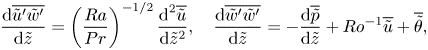 \begin{equation} \frac{\textrm{d}\overline{\tilde{u}'\tilde{w}'}}{\textrm{d}\tilde{z}} = \left( \frac{Ra}{Pr} \right)^{-1/2} \frac{\textrm{d}^{2}\overline{\tilde{u}}}{\textrm{d}\tilde{z}^{2}}, \quad \frac{\textrm{d}\overline{\tilde{w}'\tilde{w}'}}{\textrm{d}\tilde{z}} = -\frac{\textrm{d}\overline{\tilde{p}}}{\textrm{d}\tilde{z}} + Ro^{-1} \overline{\tilde{u}} + \overline{\tilde{\theta}}, \end{equation}
where (3.1a,b) are the averaged  $u$- and
  $w$-momentum equations, respectively. If we integrate (3.1a) from
  $\tilde {z}=0$ to an arbitrary
  $\tilde {z}$, we obtain
  $\overline {\tilde {u}'\tilde {w}'} = ( Ra/Pr )^{-1/2}\,\textrm {d}\overline {\tilde {u}}/\textrm {d}\tilde {z} - (Ra/Pr )^{-1/2}\,\textrm {d}\overline {\tilde {u}}/\textrm {d}\tilde {z}\vert _{\tilde {z}=0}$. We can draw two conclusions from this equation. First, considering this equation at
  $\tilde {z}=1$ (top wall), we obtain
  $\textrm {d}\overline {\tilde {u}}/\textrm {d}\tilde {z}\vert _{\tilde {z}=0} = \textrm {d}\overline {\tilde {u}}/\textrm {d}\tilde {z}\vert _{\tilde {z}=1}$, hence the wall shear stresses at the top and bottom walls have equal magnitudes but opposite signs (
 $\bar {\tau }_{w_{top}} = -\rho _o \nu \, \textrm {d}\bar {u}/\textrm {d}z\vert _{z=H}, \bar {\tau }_{w_{bot}} = \rho _o \nu \,\textrm {d}\bar {u}/\textrm {d}z\vert _{z=0}$). Second, if we further integrate this equation from
  $\tilde {z}=0$ to
  $1$, we obtain
  $C_{f_{top}} = C_{f_{bot}} = 2| \int _0^{1} \overline {\tilde {u}'\tilde {w}'}\,\textrm {d}\tilde {z} |$, hence the wind momentum is adjusted by the integral of Reynolds shear stress. These two conclusions must be valid for all values of
  $Ro^{-1}$ (3.1a,b). The first conclusion can be confirmed from figure 8(b), comparing the mean velocity profiles near the bottom wall (solid line) and top wall (dot-circled line). The profiles within a distance of
  $20$ wall units from the end walls are identical to each other, even at
  $Ro^{-1} = 1$ (solid black line), where the antisymmetric wind is broken. From the second conclusion, the Coriolis and buoyancy forces must generate the wind through
  $\overline {u' w'}$. Inspecting (3.1b) shows that the Coriolis force (
 $Ro^{-1}\bar {u}$) and buoyancy force (
 $\bar {\theta }$) can modify the wall-normal Reynolds stress
  $\overline {w'w'}$, which in turn modifies
  $\overline {u'w'}$. At
  $Ro^{-1}_{opt} = 0.8$ (solid green line), where the wind momentum reaches maximum,
  $\overline {u'w'}$ is maximum at all heights (figure 8c). At
  $Ro^{-1}=20$ (solid grey line), the flow is laminar and
  $\overline {u'w'}$ is due to the flow unsteadiness (
 $u' = (u - \bar {u}$) is the unsteady component). Nevertheless,
  $| \int _0^{H} \overline {u'w'}\,\textrm {d}z |$ at
  $Ro^{-1} = 20$ is still smaller than its counterpart at
  $Ro^{-1}_{opt} = 0.8$.
3.3. Flow behaviour beyond the optimal Coriolis force
As discussed in § 3.1, beyond  $Ro^{-1}_{opt}$ (figure 7c,g), the strong bidirectional wind is weakened and loses its antisymmetric nature. We visualise this case (
 $Ra=10^{8}$ and
  $Ro^{-1} =1.0 > Ro^{-1}_{opt} = 0.8$) in figure 9 for a period of approximately
  $4H/U$ (indicated in the
  $xy$-plane averaged wall shear-stress
  $\tau ^{xy}_w$ history). We see that wind breaking is coincident with the formation of coherent large-scale circulations. These circulations are identified by the
  $y$-averaged spanwise vorticity
  $\omega ^{y}_y = ( \partial u^{y}/\partial z - \partial w^{y}/\partial x )$. Regions of high vorticity, hence strong circulation coincide with the regions of high Coriolis force. We can show this by taking the divergence of momentum equation (2.1b)–(2.1d),
 \begin{equation} \partial_{\tilde{x}_i \tilde{x}_j} \left( \tilde{u}_i \tilde{u}_j \right) = -\tilde{\nabla}^{2} \tilde{p} +Ro^{-1} \tilde{\omega}_y + \partial_{\tilde{z}}\tilde{\theta} \quad \quad i,j=1,2,3. \end{equation}
Equation (3.2) shows that the Coriolis term  $Ro^{-1} \tilde {\omega }_y$ is strong anywhere that
  $\widetilde {\omega _y}$ is large. In total, two circulations are formed: a strong cyclone near the top wall (marked with
  $\times$, green, corotating with the system) and a weak anticyclone in the bulk (marked with
  $+$, red, counter-rotating to the system). In figure 9(h–m), we observe that a cyclone is a quasi-two-dimensional roller that elongates in the spanwise direction. The
  $z$-location of the cyclone does not change with time, but it travels in the
  $x$-direction. The terms cyclone and anticyclone are widely used in rotating flows to identify coherent corotating or counter-rotating structures. However, they do not represent the shape of structures, e.g. columnar, plume-like or roll-like. The flow structures that we observe here as a large-scale concentrated cyclone accompanied by a field of weak anticyclones are also seen in rot_RB_slip with free-slip boundaries (Favier et al. Reference Favier, Silvers and Proctor2014; Guervilly et al. Reference Guervilly, Hughes and Jones2014). Also, recent study of rot_RB_wall with no-slip boundaries (Aguirre Guzmán et al. Reference Aguirre Guzmán, Madonia, Cheng, Ostilla-Mónico, Clercx and Kunnen2020) reveals such structures at
  $Ra \gtrsim 10^{9}$ and
  $Ro^{-1} \gtrsim 10$. However, these structures are not seen in rot_RB_cyl so far (Kunnen et al. Reference Kunnen, Stevens, Overkamp, Sun, van Heijst and Clercx2011; Favier & Knobloch Reference Favier and Knobloch2020; Shishkina Reference Shishkina2020; de Wit et al. Reference de Wit, Aguirre Guzmán, Madonia, Cheng, Clercx and Kunnen2020; Zhang et al. Reference Zhang, Van Gils, Horn, Wedi, Zwirner, Ahlers, Ecke, Weiss, Bodenschatz and Shishkina2020).

Figure 9. Visualisation of cyclones ( $\times$, green,
  $\omega ^{y}_y > 0$) and anticyclones (
 $+$, red,
  $\omega ^{y}_y < 0$) at different instantaneous times for
  $Ra=10^{8}, Ro^{-1} =1 > Ro^{-1}_{opt}$ (
 $Ro^{-1}_{opt} = 0.8$), where
  $\omega ^{y}_y = ( \partial u^{y}/\partial z - \partial w^{y}/\partial x )$ is the spanwise-averaged spanwise vorticity. The visualisation times from panel (b) to panel (g) are indicated by vertical dashed lines in the
  $\tau ^{xy}_w$ history, from left to right, where
  $\tau ^{xy}_{w_{bot}} = -\rho _o \nu \,\textrm {d}u^{xy}/\textrm {d}z\vert _{z=0}$ (solid red line) and
  $\tau ^{xy}_{w_{top}} = -\rho _o \nu \,\textrm {d}u^{xy}/\textrm {d}z\vert _{z=H}$ (solid blue line) are the instantaneous
  $xy$-plane averaged wall shear stresses. (b–g) Here
  $\omega ^{y}_y$ overlaid by the velocity vector
  $(u^{y},w^{y})/U$. (h–m) Correspond to the same flow fields in (b–g), respectively, but show the instantaneous streamwise velocity field near the top wall at
  $z/H=0.96$; the solid green line locates
  $u = 0$, enclosing the flow reversal caused by the quasi-two-dimensional cyclone. The circled red arrow on the top right indicates the system rotation direction.
To study the energy content of cyclones and anticyclones, in figure 10 we plot the premultiplied spectra of the case from figure 9, at  $Ra=10^{8}$ and
  $Ro^{-1}=1.0$. The most energetic scale (marked with
  $\times$, green in figure 10b) has the wavelength of
  $\lambda _x = H$ and is located at
  $(1-z/H)\simeq 0.05$ (
 $z/H \simeq 0.95$). This energetic scale is cyclone, marked with (
 $\times$, green) in figure 9(b–g). On the other hand, the energy content of anticyclone (located at
  $z/H \simeq 0.5$) is as low as the background turbulence. Such a clear symmetry breaking in favour of cyclone has been reported at moderately low Rossby numbers (in the order of unity), in rot_RB_slip (Favier et al. Reference Favier, Silvers and Proctor2014; Guervilly et al. Reference Guervilly, Hughes and Jones2014), forced homogeneous rotating turbulence (Smith & Waleffe Reference Smith and Waleffe1999; Smith & Lee Reference Smith and Lee2005) and decaying homogeneous rotating turbulence (Bartello, Métais & Lesieur Reference Bartello, Métais and Lesieur1994; Morize, Moisy & Rabaud Reference Morize, Moisy and Rabaud2005; Moisy et al. Reference Moisy, Morize, Rabaud and Sommeria2011). Bartello et al. (Reference Bartello, Métais and Lesieur1994), Morize et al. (Reference Morize, Moisy and Rabaud2005) and Favier et al. (Reference Favier, Silvers and Proctor2014) studied the probability density function of vorticity. They concluded that the prevalence of cyclones is due to the dominance of cyclonic small scales.

Figure 10. Streamwise premultiplied spectra for the  $u$-velocity
  $k_x E_{uu}(k_x)/U^{2} \times 10^{2}$, where
  $\lambda _x = 2{\rm \pi} /k_x$, at
  $Ra = 10^{8}$ and
  $Ro^{-1} =1.0 > Ro^{-1}_{opt} = 0.8$, the case visualised in figure 9. Here (a)
  $0\le z/H \le 0.5$ and (b)
  $0\le (1-z/H) \le 0.5$. The contour levels are increasing from
  $0.1$ to
  $1.0$ with an increment of
  $0.1$. The most energetic scale, marked with a green
  $\times$ in panel (b), highlights the energetic cyclone near the top wall.
3.4. Local ‘turbulence’ Rossby number
In our system, cyclones and anticyclones are formed at different transitional  $Ro^{-1}$, depending on
  $Ra$. Also, at a fixed
  $Ra$, the transitional
  $Ro^{-1}$ depends on the rotating system. For example, in Favier et al. (Reference Favier, Silvers and Proctor2014) at
  $Ra = 10^{7}$ the transitional
  $Ro^{-1}$ is
  $3.1$ (while it is
  $1.2$ in our system), and at
  $Ra=10^{8}$ it is
  $1.8$ (and
  $1.0$ in our system). In both systems, the transitional
  $Ro^{-1}$ decreases as
  $Ra$ increases, but the transitional values are different. Favier et al. (Reference Favier, Silvers and Proctor2014) consider rotating Rayleigh–Bénard convection with free-slip hot and cold boundaries (rot_RB_slip in table 1), while we consider centrifugal convection (figure 1). The
  $Ra$ and system dependency of transitional
  $Ro^{-1}$ is because
  $Ro^{-1} \equiv 2\varOmega H/U$ characterises the Coriolis force over the entire system. However, the Coriolis force is locally distributed differently, depending on
  $Ra$ and the rotating system. Therefore, the formation of a cyclone as a local phenomenon, must be characterised based on a local measure of inverse Rossby number (
 $Ro^{-1}_L$).
Hopfinger et al. (Reference Hopfinger, Browand and Gagne1982) defined  $Ro^{-1}_L$ based on local turbulent velocity scale and integral length scale. They observed the formation of cyclones when locally
  $Ro^{-1}_L$ increases to approximately
  $5$. Following Hopfinger et al. (Reference Hopfinger, Browand and Gagne1982), other studies (table 3) made the same observation at nearly the same transitional
  $Ro^{-1}_L$. The studies in table 3 are both experimental and numerical, and consider different rotating systems. However, they all report a transitional
  $Ro^{-1}_L$ close to
  $5$. In the rest of this subsection, first, we examine whether there is a unified transitional
  $Ro^{-1}_L$ for our rotating system, independent of
  $Ra$. Then, by taking the advantage of this unified value, we attempt to arrive at a relation between
  $Ro^{-1}_{opt}$ (before the cyclone formation) and
  $Ra$. We define local ‘turbulence’ inverse Rossby number
  $Ro^{-1}_L \equiv (2\varOmega \bar {\mathcal {K}})/\overline {\varepsilon _u}$ based on eddy turnover time
  $\bar {\mathcal {K}}/ \overline {\varepsilon _u}$, where
  $\bar {\mathcal {K}}$ is the turbulent kinetic energy.
Table 3. Summary of the previous studies that have reported the transitional local inverse Rossby number  $Ro^{-1}_L$, based on turbulent velocity scale and integral length scale. All the studies are experimental except Godeferd & Lollini (Reference Godeferd and Lollini1999).

In figure 11 we plot the profiles of  $Ro^{-1}_L$ at
  $Ra=10^{7}$ (figure 11e) to
  $10^{10}$ (figure 11h), and
  $Ro^{-1}=0.3$ (solid red line) to
  $2.0$ (dashed blue line). We also add the plane and time averaged streamwise velocity profiles
  $\bar {u}$ (figure 11a–d). We aim to see if there is any relation between
  $Ro^{-1}_L$ and wind breaking, i.e. when the antisymmetric
  $\bar {u}$ profile is deformed. At each
  $Ra$, we mark the deformed
  $\bar {u}$ profiles and their corresponding
  $Ro^{-1}_L$ profiles. The profiles marked with a blue
  $\bullet$ indicate the stage where the
  $\bar {u}$ profile still preserves its (
 $\mathcal {S}$) shape, while the profiles marked with a hot magenta
  $\blacklozenge$ indicate the stage where the
  $\bar {u}$ profile is completely deformed. We compare these two stages at
  $Ra=10^{10}$ in figure 12. These stages correspond to the solid green line and solid black line in figure 11(d,h). The stage marked with a blue
  $\bullet$ (figure 12a) is slightly beyond
  $Ro^{-1}_{opt}$ and cyclone is near the wall. The stage marked with a hot magenta
  $\blacklozenge$ (figure 12b) is further beyond
  $Ro^{-1}_{opt}$ and the cyclone has migrated to the bulk. As a result, the
  $\bar {u}$ profile direction is reversed (solid black line in figure 11d). We see similar trend in the
  $\bar {u}$ profile at
  $Ra = 10^{8}$ (figure 8a). The reversal in
  $\bar {u}$ from
  $Ro^{-1}=1$ (solid black line) to
  $20$ (solid grey line) is due to the migration of cyclone to the bulk.

Figure 11. Profiles of the plane and time averaged streamwise velocity  $\bar {u}$ (a–d) and local inverse Rossby number
  $Ro^{-1}_L \equiv 2\varOmega \bar {\mathcal {K}}/ \overline {\varepsilon _u}$ (e–h), at
  $Ra = 10^{7}$ (a,e),
  $10^{8}$ (b,f),
  $10^{9}$ (c,g) and
  $10^{10}$ (d,h). Here
  $Ro^{-1} = 0.3$ (solid red line),
  $0.5$ (solid blue line),
  $0.6$ (solid magenta line),
  $0.8$ (solid green line),
  $1.0$ (solid black line) and
  $2.0$ (dashed blue line). The vertical dashed-dotted grey line in the bottom row locates the transitional
  $Ro^{-1}_L=4.0$, beyond which the cyclone is formed. All the
  $\bar {u}$ profiles that are deformed from their antisymmetric shape are marked with (
 $\bullet$, blue;
  $\blacklozenge$, hot magenta), as well as their
  $Ro^{-1}_L$ profiles. Those marked with a blue
  $\bullet$ are partially deformed (still preserve their
  $\mathcal {S}$ shape). Those marked with a hot magenta
  $\blacklozenge$ are completely deformed. The markers are placed at the maximum
  $Ro^{-1}_L$.

Figure 12. Instantaneous visualisation of  $\omega ^{y}_y = ( \partial u^{y}/\partial z - \partial w^{y}/\partial x )$, spanwise-averaged spanwise vorticity, overlaid by the streamlines of
  $(u^{y},w^{y})/U$ and local inverse Rossby number
  $Ro^{-1}_L \equiv 2\varOmega \bar {\mathcal {K}}/\overline {\varepsilon _u}$, at
  $Ra = 10^{10}$ and (a)
  $Ro^{-1} = 0.8$ and (b)
  $Ro^{-1}=1.0$. Panels (a,b) correspond to the profiles (solid green line) and (solid black line) in figure 11(d,h), respectively. The vertical and bottom horizontal axes are the wall-normal
  $z/H$ and streamwise
  $x/H$ coordinates, respectively, for the vorticity field and velocity vector. The top horizontal axis is
  $Ro^{-1}_L$ for the overlaid profiles of
  $Ro^{-1}_L$ versus
  $z/H$. The circled red arrow on the right-hand side indicates the system rotation direction.
Considering all the marked  $Ro^{-1}_L$ profiles in figure 11(e–h), wind breaking starts (cyclone appears) once
  $Ro^{-1}_L \gtrsim 4.0$. This transitional
  $Ro^{-1}_L \simeq 4.0$ is close to the value of
  $5.0$ reported in the literature (table 3). The region of
  $Ro^{-1}_L > 4$ locates a cyclone (figure 12) with maximum
  $Ro^{-1}_L$ near the core of the cyclone. Slightly beyond
  $Ro^{-1}_{opt}$ (marked with
  $\bullet$, blue in figure 11), the maximum
  $Ro^{-1}_L$ also coincides with the peak of
  $\bar {u}$. Because the cyclone is small (figure 12a), hence its core (the maximum
  $Ro^{-1}_L$) and its edge (the peak of
  $\bar {u}$) are close to each other. Further beyond
  $Ro^{-1}_{opt}$ (marked with
  $\blacklozenge$, hot magenta in figure 11), the maximum
  $Ro^{-1}_L$ does not coincide with the peak of
  $\bar {u}$. Because the cyclone is large (figure 12b), hence its core and its edge are distant from each other.
Figure 11(e–h) shows that  $Ro^{-1}_L$ monotonically increases, by increasing
  $Ra$ or
  $Ro^{-1}$, up to
  $Ro^{-1}_L \simeq 4.0$. We reaffirm this behaviour in figure 13, plotting
  $Ro^{-1}_L$ at the maximum
  $\bar {u}$ (
 $Ro^{-1}_{L_{\bar {u}_{max}}}$) versus
  $Ra$ (figure 13a) and
  $Ro^{-1}$ (figure 13b). Here
  $Ro^{-1}_{L_{\bar {u}_{max}}}$ increases with a power of
  $Ra$ or
  $Ro^{-1}$ up to
  $Ro^{-1}_{L_{\bar {u}_{max}}} \simeq 4.0$ (marked with a dashed-dotted grey line in figure 13a,b). We can support this power-law behaviour through scaling arguments for
  $\bar {\mathcal {K}}_{\bar {u}_{max}}$ and
  $\bar {\varepsilon }_{\bar {u}_{max}}$ (
 $Ro^{-1}_{L_{\bar {u}_{max}}} \equiv 2\varOmega \bar {\mathcal {K}}_{\bar {u}_{max}}/ \bar {\varepsilon }_{\bar {u}_{max}}$). Deardorff (Reference Deardorff1970) found
  $w_* \equiv ( g \beta \kappa \varDelta Nu )^{1/3} = \kappa /H (Pr\,Nu\,Ra)^{1/3}$ as a suitable velocity scale for the r.m.s. of wall-normal velocity fluctuations
  $w_{rms}$ in Rayleigh–Bénard convection. Xie, Hu & Xia (Reference Xie, Hu and Xia2019) observed that
  $w_{rms}/w_*$ weakly depends on
  $Ra$ (
 $\sim Ra^{0.07\pm 0.02}$). Here, our data of
  $\bar {\mathcal {K}}_{\bar {u}_{max}}$ scale well with
  $w^{2}_*$, without
  $Ra$ correction (figure 13c). One possibility could be due to our unbounded (periodic) domain compared with the bounded (cylindrical or cubic) domains in Xie et al. (Reference Xie, Hu and Xia2019). Another possibility could be due to the Coriolis force that is absent in Rayleigh–Bénard convection of Xie et al. (Reference Xie, Hu and Xia2019). Our data of
  $\bar {\varepsilon }_{\bar {u}_{max}}$ scale well with
  $w^{3}_*/H=\nu ^{3} H^{-4} Nu Ra Pr^{-2}$ (figure 13d). Because the volume and time averaged dissipation rate is
  $\left \langle \varepsilon _u \right \rangle \simeq w^{3}_*/H$ in the inertia-dominated regime (
 $Nu \gg 1$), see § 2.2. With these scales for
  $\bar {\mathcal {K}}_{\bar {u}_{max}}$ and
  $\bar {\varepsilon }_{\bar {u}_{max}}$, we obtain
  $Ro^{-1}_{L_{\bar {u}_{max}}} \propto Pr^{1/6} Ra^{1/6} Ro^{-1} Nu^{-1/3}$. Considering
  $Nu$ versus
  $Ra$ (figure 5) for
  $Ro^{-1}<1$, it nearly falls into the classical regime scaling, i.e.
  $Nu \propto Ra^{0.29}$ (Scheel & Schumacher Reference Scheel and Schumacher2016). Substituting for
  $Nu$ and
  $Pr = 0.7$, we obtain
  $Ro^{-1}_{L_{\bar {u}_{max}}} \propto 0.94 Ra^{0.07} Ro^{-1}$. Figures 13(a), dashed lines, and 13(b), solid lines, show the good agreement between this power-law relation and the simulation data up to
  $Ro^{-1}_L \le 4$.

Figure 13. Variation of  $Ro^{-1}_L$ at the maximum
  $\bar {u}$ (
 $Ro^{-1}_{L_{\bar {u}_{max}}}$): (a) as a function of
  $Ra$ for different
  $Ro^{-1}$ values and (b) as a function of
  $Ro^{-1}$ for different
  $Ra$ values. The horizontal line (dashed-dotted grey line) in panels (a,b) mark
  $Ro^{-1}_{L_{\bar {u}_{max}}} = 4$, above which the cyclone forms. The symbols are from the simulations at
  $Ro^{-1}=0.3$ (
 $\square$, red),
  $0.5$ (
 $\triangle$, blue),
  $0.6$ (+, magenta),
  $0.8$ (*, green),
  $1.0$ (
 $\circ$, black). The symbols filled with a black dot are at
  $Ro^{-1}_{opt}$ at each
  $Ra$. The fitting dashed lines in panel (a) and solid lines in panel (b) are the theoretical relation
  $Ro^{-1}_{L_{\bar {u}_{max}}} \simeq 0.94 Ra^{0.07} Ro^{-1}$. This relation is derived based on the scaling arguments for
  $\bar {\mathcal {K}}_{\bar {u}_{max}} \propto w^{2}_*$,
  $\bar {\varepsilon }_{\bar {u}_{max}} \propto w^{3}_*/H$,
  $Nu \propto Ra^{0.29}$ and
  $Pr=0.7$ (see the text), where
  $w_* \equiv \kappa /H ( Pr Nu Ra )^{1/3}$. Panels (c,d) verify the scaling arguments for
  $\bar {\mathcal {K}}_{\bar {u}_{max}}$ and
  $\bar {\varepsilon }_{\bar {u}_{max}}$, respectively. For clarity, in (c,d) we only show the data points with
  $Ro^{-1}_L < 4$ (below dashed-dotted grey line in panel a). The dotted line in panel (c) indicates the scaling
  $\bar {\mathcal {K}}_{\bar {u}_{max}} \propto w^{2}_* Ra^{0.14}$ based on the correction by Xie et al. (Reference Xie, Hu and Xia2019).
We can predict  $Ro^{-1}_{opt}$ at each
  $Ra$ using this power-law. The data points at
  $Ro^{-1}_{opt}$ (filled with black dots in figure 13a), fall at
  $Ro^{-1}_{L_{\bar {u}_{max}}}\simeq 3.0$. After substituting for
  $Ro^{-1}_{L_{\bar {u}_{max}}} = 3.0$ and
  $Ro^{-1} = Ro^{-1}_{opt}$ in the power-law relation and some recasting, we arrive at
  $Ro^{-1}_{opt} \simeq 3.19 Ra^{-0.07}$. This relation confirms the slight variation of
  $Ro^{-1}_{opt}$ with
  $Ra$ (figure 6a).
Our approach in this subsection is similar to the one by King et al. (Reference King, Stellmach, Noir, Hansen and Aurnou2009); to identify the transition from the buoyancy (inertia) dominated to the Coriolis dominated regime. King et al. (Reference King, Stellmach, Noir, Hansen and Aurnou2009) focus on rot_RB_wall (table 1), while we consider centrifugal convection. Both in King et al. (Reference King, Stellmach, Noir, Hansen and Aurnou2009) and here, we relate the transition to a local phenomenon. In King et al. (Reference King, Stellmach, Noir, Hansen and Aurnou2009) the transition occurs in the Ekman layer. They explain the transition through the competition between the Ekman layer and thermal boundary layer. Here, the transition occurs in the bulk, i.e. the locale of cyclone. Therefore, we explain the transition through  $Ro^{-1}_L \equiv 2\varOmega \bar {\mathcal {K}}/\bar {\varepsilon }_u$, i.e. the competition between the system rotation time scale and the turbulence time scale.
3.5. Flow behaviour at very large Coriolis force
At the very large  $Ro^{-1} = 20$ (figure 7d,h), turbulence is suppressed and the flow becomes two-dimensional and laminar-like. In figure 14, we visualise this case over a period of
  $150H/U$. In the top row, we visualise
  $\tilde {\theta }$ overlaid by the
  $(\tilde {u},\tilde {w})$ streamlines. In the bottom row, we visualise the vorticity field
  $\tilde {\omega }_y = ( \partial _{\tilde {z}} \tilde {u} - \partial _{\tilde {x}} \tilde {w} )$. We locate the core of cyclones (
 $\blacklozenge$, green) and anticyclones (
 $\bullet$, red) based on the core of streamlines, i.e.
  $(\tilde {u},\tilde {w}) \simeq (0,0)$. Figure 14 shows that at the very large
  $Ro^{-1}$, the cyclone in the bulk and anticyclones near the walls become equally strong. The stabilisation of both cyclones and anticyclones at very large
  $Ro^{-1}$ is observed in rotating Rayleigh–Bénard convection with free-slip boundaries (rot_RB_slip). For instance, refer to figure 3 in Stellmach et al. (Reference Stellmach, Lischper, Julien, Vasil, Cheng, Ribeiro, King and Aurnou2014) (
 $Ra \simeq 2\times 10^{11}, Ro^{-1} \simeq 23$) or figure 2 in Guervilly et al. (Reference Guervilly, Hughes and Jones2014) (
 $Ra \simeq 8 \times 10^{8}, Ro^{-1} \simeq 7$). However, in those studies turbulence is not completely suppressed. This difference might be due to their different flow set-up (rot_RB_slip in table 1) compared with our set-up (centrifugal convection).

Figure 14. Flow visualisation at different times  $tU/H$ for
  $Ra=10^{8}, Ro^{-1} =20$. Note that the flow is two-dimensional, i.e. depends on
  $x,z$ only. The visualisation times from panel (b) to panel (g) are indicated by vertical dashed lines in the plane-averaged wall shear stress
  $\tau ^{xy}_w$ history. The solid red line and solid blue line are, respectively, the bottom and top wall,
  $\tau ^{xy}_w$. (b–g) Temperature field
  $\tilde {\theta } = \theta /\varDelta$ overlaid by the streamlines. (h–m) Correspond to the same flow fields in (b–g), respectively, but show the vorticity
  $\tilde {\omega }_y = (H/U)(\partial u/\partial z - \partial w/\partial x )$. The core of cyclone (
 $\blacklozenge$, green,
  $\omega _y > 0$) and anticyclone (
 $\bullet$, red,
  $\omega _y < 0$) are marked based on
  $(u,w)\simeq (0,0)$, i.e. the core of streamlines. The circled red arrow on the top right indicates the system rotation direction.
In figure 14(b–g), the cyclone has almost a uniform zero temperature. Also, the anticyclones near the bottom and top walls have a uniform hot and cold temperature, respectively. To explain this phenomenon, in figure 15 we study different terms of  $u$- and
  $w$-momentum equations. The diffusion terms are negligible and the momentum balance is primarily between the pressure gradient (figure 15c,g) and Coriolis force (figure 15d,h). This balance is known as the geostrophic balance (Greenspan Reference Greenspan1968), leading to the geostrophic regime. In this regime, there is a drop in
  $Nu$ (King et al. Reference King, Stellmach, Noir, Hansen and Aurnou2009; Schmitz & Tilgner Reference Schmitz and Tilgner2009; Ecke & Niemela Reference Ecke and Niemela2014), also seen in our case at
  $Ra=10^{8}$ from
  $Ro^{-1} = 1$ to
  $20$ (
 $\circ$, black to
  $\triangledown$, olive green, in figure 5). This regime also appears in rapidly rotating Rayleigh–Bénard convection, in all the common set-ups of this flow (table 1). To name a few for rot_RB_wall see Julien et al. (Reference Julien, Legg, McWilliams and Werne1996b), Kunnen et al. (Reference Kunnen, Clercx and Geurts2006) and King et al. (Reference King, Stellmach, Noir, Hansen and Aurnou2009, Reference King, Stellmach and Aurnou2012); for rot_RB_slip see Stellmach et al. (Reference Stellmach, Lischper, Julien, Vasil, Cheng, Ribeiro, King and Aurnou2014) and Guervilly et al. (Reference Guervilly, Hughes and Jones2014); and for rot_RB_cyl see Vorobieff & Ecke (Reference Vorobieff and Ecke2002), Ecke & Niemela (Reference Ecke and Niemela2014), Ecke (Reference Ecke2015) and Rajaei, Kunnen & Clercx (Reference Rajaei, Kunnen and Clercx2017). However, the flow phenomenology evolves differently among these three systems (Kunnen et al. Reference Kunnen, Ostilla-Mónico, van der Poel, Verzicco and Lohse2016; Zhang et al. Reference Zhang, Van Gils, Horn, Wedi, Zwirner, Ahlers, Ecke, Weiss, Bodenschatz and Shishkina2020). In planetary flows, such as atmospheric or ocean circulations,
  $Ro^{-1}$ can go beyond
  $10$ (Kundu & Cohen Reference Kundu and Cohen1990) and geostrophic balance occurs.

Figure 15. Terms of the  $u$-momentum (a–d) and
  $w$-momentum equation (e–i) at
  $Ra=10^{8}$ and
  $Ro^{-1} = 20$. Note that the flow is two-dimensional, i.e. depends on
  $x,z$ only. Here (a,e)
  $\partial \tilde {u}_i/\partial \tilde {t}$; (b,f)
  $\partial \tilde {u}_i \tilde {u}_j/\partial \tilde {x}_j$; (c,g)
  $-\partial \tilde {p}/\partial \tilde {x}_i$; (d,h)
  $-Ro^{-1}\epsilon _{ijk} \tilde {u}_k$, where
  $\epsilon _{ijk}$ is the permutation tensor; and (i)
  $\tilde {\theta }$. The diffusion terms are negligible, i.e.
  $(Pr/Ra)^{1/2}(\partial ^{2} \tilde {u}_i/\partial \tilde {x}_j^{2}) \simeq O(10^{-2})$.
Although the geostrophic balance is between the Coriolis force and pressure gradient, in our system we cannot ignore the transient (figure 15a,e) and advection terms (figure 15b,f), as figure 14 shows that this is an unsteady problem. Also we cannot ignore the buoyancy term (figure 15i), as there would be no flow without this term. We also assessed the terms of the temperature transport equation (2.1e). Similar to momentum, the diffusion terms are orders of magnitude smaller than the transient and advection terms. Therefore, the governing equations ((2.1a)–(2.1e)) are simplified to
 \begin{equation} \partial_{\tilde{x}} \tilde{u} + \partial_{\tilde{z}} \tilde{w} =0, \quad D_{\tilde{t}} \tilde{u} = -\partial_{\tilde{x}} \tilde{p} -Ro^{-1} \tilde{w}, \quad D_{\tilde{t}} \tilde{w} = -\partial_{\tilde{z}} \tilde{p} +Ro^{-1} \tilde{u} + \tilde{\theta}, \quad D_{\tilde{t}} \tilde{\theta} = 0, \end{equation}
where  $D_{\tilde {t}}\left \langle \cdot \right \rangle = \partial _{\tilde {t}} \left \langle \cdot \right \rangle + \tilde {u}\partial _{\tilde {x}} \left \langle \cdot \right \rangle + \tilde {w}\partial _{\tilde {z}} \left \langle \cdot \right \rangle$ is the material derivative. The material derivative of a property implies the rate of change of that property as we track a cyclone or anticyclone. We recast (3.3a–d) in terms of stream function
  $\tilde {\psi }$ (
 $\tilde {u} = \partial _{\tilde {z}} \tilde {\psi }, \tilde {w} = - \partial _{\tilde {x}} \tilde {\psi }$) and
  $\tilde {\omega }_y$ as follows:
 \begin{equation} \partial^{2}_{\tilde{x}\tilde{x}} \tilde{\psi} + \partial^{2}_{\tilde{z}\tilde{z}} \tilde{\psi} =\tilde{\omega}_y, \quad D_{\tilde{t}} \tilde{\omega}_y = -\partial_{\tilde{x}} \tilde{\theta}, \quad D_{\tilde{t}} \tilde{\theta} = 0. \end{equation}
A similar set of equations is solved for quasi-geostrophic flows to study the interaction of cyclones and anticyclones with themselves (Reinaud, Dritschel & Koudella Reference Reinaud, Dritschel and Koudella2003; Dritschel, Reinaud & McKiver Reference Dritschel, Reinaud and McKiver2004; Reinaud & Carton Reference Reinaud and Carton2016) or with the wall (Deremble, Johnson & Dewar Reference Deremble, Johnson and Dewar2017; Venaille Reference Venaille2020). Equation (3.4c) justifies figure 14(b–g); the temperature of cyclone and anticyclones does not change with time. Also, (3.4b) justifies the uniform  $\tilde {\theta }$ within each cyclone and anticyclone. Considering figure 14(h–m), the vorticity of cyclone and anticyclones is materially conserved, i.e.
  $(D_{\tilde {t}} \tilde {\omega }_y)_{cyclone} \simeq (D_{\tilde {t}} \tilde {\omega }_y)_{anticyclone} \simeq 0$. Therefore, from (3.4b) we expect
  $(\partial _{\tilde {x}} \tilde {\theta })_{cyclone} \simeq (\partial _{\tilde {x}} \tilde {\theta })_{anticyclone} \simeq 0$, i.e.
  $\tilde {\theta }$ is uniform within each cyclone or anticyclone.
3.6. Towards logarithmic boundary layers
In § 3.1 we showed the remarkable feature of this centrifugal system in forming a bidirectional wind with the maximum momentum at  $Ro^{-1}_{opt}$, presumably helping the boundary layer transition to the turbulent Prandtl–von Kármán type, as hypothesised by Kraichnan (Reference Kraichnan1962). In this subsection, we demonstrate this feature by studying the structure of the wind as
  $Ra$ increases. The value of
  $Ro^{-1}_{opt}$ changes with
  $Ra$, from
  $1.0$ at
  $Ra=10^{7}$, to
  $0.6$ at
  $Ra=10^{10}$ (figure 6b). Here, we fix
  $Ro^{-1}$ at
  $0.8$, a value slightly smaller or larger than
  $Ro^{-1}_{opt}$, so that the system still generates a high momentum wind. In figure 16, we study the mean velocity and temperature profiles and r.m.s. of their fluctuations from the top wall to the domain midheight, as
  $Ra$ increases. To study the distance to a turbulent boundary layer, in figure 16 in addition to the law of the wall for Prandtl–von Kármán type boundary layer (dashed-dotted blue line), we overlay the mean and r.m.s. velocity profiles by their counterparts from the DNS of turbulent channel flow (solid red line) at
  $Re_{\tau } \simeq 180$ (Lee & Moser Reference Lee and Moser2015), based on channel half-height, and we overlay the temperature profiles by their counterparts from the DNS of turbulent channel flow with passive scalar (dotted red line) at
  $Re_{\tau } = 180$ and
  $Pr=0.71$ (Kim & Moin Reference Kim and Moin1989). We choose this value of
  $Re_{\tau }$ for comparison, because in our system at the highest
  $Ra=10^{10}$ (solid black line in figure 16a),
  $Re_{\tau }$ reaches approximately
  $155$ based on the velocity boundary-layer thickness. We define the boundary-layer thickness where
  $| \bar {u} |^{+}$ is maximum.

Figure 16. Profiles of the (a) absolute mean velocity  $|\bar {u}|$, (b) mean temperature
  $(\bar {\theta }-\theta _L)=(\bar {\theta }+\varDelta /2)$, (c) r.m.s. of velocity fluctuation
  $u_{rms} = \sqrt {\overline {u'^{2}}}$ and (d) r.m.s. of temperature fluctuation
  $\theta _{rms} = \sqrt {\overline {\theta '^{2}}}$ from the top wall to the domain midheight,
  $0 \le (H-z) \le H/2$, at
  $Ro^{-1}=0.8$ and
  $Ra = 10^{7}$ (dotted black line),
  $10^{8}$ (dashed black line),
  $10^{9}$ (dashed-dotted black line) and
  $10^{10}$ (solid black line). We normalise
  $|\bar {u}|$ and
  $u_{rms}$ by the top wall friction velocity
  $u_{\tau _{top}}$. We normalise
  $(\bar {\theta }-\theta _L)$ and
  $\theta _{rms}$ by
  $\theta _{\tau _{top}} = -\kappa (\textrm {d}\bar {\theta }/\textrm {d}z\vert _{z=H})/u_{\tau _{top}}$. In panel (a), we plot law of the wall (dashed-dotted blue line) in the viscous sublayer
  $\bar {u}^{+} =z^{+}$ and log layer (Prandtl–von Kármán profile)
  $\bar {u}^{+} = (1/0.41) \ln (z^{+})+5.2$ (Yaglom Reference Yaglom1979). In panel (b), we plot Prandtl–von Kármán type temperature profile for fully turbulent flow (dashed-dotted blue line) in the viscous sublayer
  $\bar {\theta }^{+} =Pr z^{+}$, and log layer
  $\bar {\theta }^{+} = (0.85/0.41) \ln (z^{+})+3.8$ (Yaglom Reference Yaglom1979). In panels (a,c), we add DNS of channel flow by Lee & Moser (Reference Lee and Moser2015) (solid red line) at
  $Re_{\tau } \simeq 180$. In panels (b,d), we add DNS of channel flow by Kim & Moin (Reference Kim and Moin1989) (dotted red line) at
  $Re_{\tau } \simeq 180$ with passive scalar at
  $Pr = 0.71$. The logarithmic fitting line (dashed hot magenta line) has the slope
  $1/0.41$ in panel (a) and has the slope
  $1/4.0$ in panel (b). In panel (a), the velocity boundary layer thickness is located by (
 $\circ$, red).
The  $\bar {u}^{+}$ profiles (figure 16a) progress towards Prandtl–von Kármán (logarithmic) behaviour as
  $Ra$ increases. Nevertheless, full collapse on the logarithmic law, corresponding to a fully turbulent wall-bounded flow, is not reached yet at
  $Ra=10^{10}$ (solid black line in figure 16a). A narrow logarithmic region (dashed magenta line) with a slope of
  $1/0.41$ starts to appear from
  $Ra=10^{9}$ (dashed-dotted black line in figure 16a). This is consistent with the two-dimensional Rayleigh–Bénard simulation of Zhu et al. (Reference Zhu, Varghese, Stevens, Verzicco and Lohse2018) who observed the emergence of the logarithmic slope
  $1/0.41$ in the mean velocity profiles before the ultimate regime (
 $Ra< 10^{13}$). They also observed a much shallower logarithmic slope (approximately
  $1/4$) in their temperature profiles compared with what is expected in a fully turbulent boundary layer (
 $0.84/0.41 \simeq 1/0.48$). We observe similar behaviour in the
  $\bar {\theta }^{+}$ profiles in figure 16(b), considering the fitting lines (dashed magenta line) with a slope of
  $1/4.0$.
From figure 16(a,b), it appears that the mean velocity profiles approach the fully turbulent counterpart faster than the mean temperature profiles. Similar behaviour is seen in the r.m.s. profiles (figure 16c,d). Both  $u_{rms}$ and
  $\theta _{rms}$ profiles yield an inner peak near the wall. The inner peak in the
  $u^{+}_{rms}$ profiles (figure 16c) is approximately
  $3.0$ at all values of
  $Ra$, which is close to the DNS of channel flow (solid red line). As
  $Ra$ increases, the location of the
  $u^{+}_{rms}$ inner peak approaches the one corresponding to the fully turbulent channel flow (solid red line). On the other hand, the inner peak of the
  $\theta ^{+}_{rms}$ profiles (figure 16d) is smaller than the fully turbulent counterpart (dotted red line), even at the highest value of
  $Ra = 10^{10}$ (solid black line in figure 16d).
Our observations from figure 16 give indications for the onset of the transition to turbulence in the velocity boundary layer at  $Ra= 10^{10}$. We visualise this transition in figure 17, showing the instantaneous field of
  $u$ at
  $15$ wall units away from the top wall. We observe the streak-like structures at
  $Ra=10^{10}$ (figure 17d), similar to a fully turbulent boundary layer. The green square with an area of
  $500 \times 500$ wall units highlights the approximately
  $100$ wall units spanwise spacing between the near-wall streaks, as in a turbulent wall-bounded flow (Kline et al. Reference Kline, Reynolds, Schraub and Runstadler1967). We also see the transition to turbulence in the spectral distribution of Reynolds shear-stress near the top wall (figure 18). We plot the spectrograms of
  $\overline {u' w'}$ at
  $Ro^{-1}=0.8$ and
  $Ra$ from
  $10^{7}$ (figure 18a) to
  $10^{10}$ (figure 18d). In figure 18(d) we overlay the spectrogram by the one from the DNS of turbulent channel flow (Lee & Moser Reference Lee and Moser2015) at
  $Re_{\tau } \simeq 180$ (solid red line). As we observe, the spectral distribution of the near-wall region at
  $Ra=10^{10}$ is similar to that of a turbulent channel flow. The spacing of
  $100$ wall units between the energetic near-wall streaks (figure 17d) can also be interpreted from the near-wall energetic mode (marked by ‘+’ in figure 18d), at
  $(H-z)^{+} \simeq 20$ and
  $\lambda ^{+}_y \simeq 100$. This subsection supports our earlier conjecture that the bidirectional wind helps the boundary layer transition to turbulent, hence the transition to the ultimate regime.

Figure 17. Instantaneous fields of  $u$ at a distance of
  $15$ wall units from the top wall at
  $Ro^{-1}=0.8$ and
  $Ra = 10^{7}$ (a),
  $10^{8}$ (b),
  $10^{9}$ (c) and
  $10^{10}$ (d). The green square in panel (d) encloses an area of
  $500\times 500$ wall units, encompassing approximately five streaks in the spanwise direction.

Figure 18. Premultiplied spectra of Reynolds shear stress  $k_y E_{uw}(k_y)/u^{2}_{\tau }$ for
  $0\le (1-z/H) \le 0.5$, where
  $\lambda _y = 2{\rm \pi} /k_y$, for the cases shown in figure 17 at
  $Ro^{-1}=0.8$ and
  $Ra =$ (a)
  $10^{7}$, (b)
  $10^{8}$, (c)
  $10^{9}$ and (d)
  $10^{10}$. The horizontal line in each plot marks the height where
  $|\bar {u}|$ is maximum in figure 16(a). Panel (d) is overlaid by
  $k_y E_{uw}(k_y)/u^{2}_{\tau }$ from the DNS of channel flow (Lee & Moser Reference Lee and Moser2015) at
  $Re_{\tau } \simeq 180$ (solid red line). The near-wall energetic mode is marked by a +, corresponding to the near-wall streak-like structures in figure 17(d). The contour levels increase from
  $-0.8$ to
  $0.8$ with an increment of
  $0.1$.
4. Conclusions
Detailed DNS and analysis of centrifugal buoyancy-driven convection has been carried out with a focus on the effect of the Coriolis force. The inverse Rossby number  $Ro^{-1}$ was varied from zero to
  $20$, the Rayleigh number
  $Ra$ from
  $10^{7}$ to
  $10^{10}$ and the Prandtl number was fixed at
  $Pr=0.7$, corresponding to air. Our range of
  $Ro^{-1}$ covered the regimes related to the turbomachinery,
  $Ro^{-1} \sim O(1)$, and geophysical flows,
  $Ro^{-1} \gg 1$.
The results show that below an optimal  $Ro^{-1}_{opt}$, the Coriolis and buoyancy force interaction form a bidirectional wind. The value of
  $Ro^{-1}_{opt}$ decreases from approximately
  $1.0$ to
  $0.6$, as
  $Ra$ increases from
  $10^{7}$ to
  $10^{10}$. At
  $Ro^{-1}_{opt}$, the wind momentum reaches its maximum, leading to a maximal
  $C_f$ and a minimal
  $Nu$. Just beyond
  $Ro^{-1}_{opt}$, the Coriolis force locally dominates. It weakens the wind and forms a large-scale cyclone. At
  $Ro^{-1} \gg Ro^{-1}_{opt}$, the Coriolis force fully dominates. It balances the pressure gradient (geostrophic balance), laminarises the flow and stabilises both cyclones and anticyclones.
The flow regimes have both similarities and differences to those in rotating Rayleigh–Bénard convection. The differences are due to the different axis of rotation and boundary conditions. In rotating Rayleigh–Bénard convection, optimal transport ( $Ro^{-1}_{opt}$) occurs only if the hot and cold boundaries are no-slip (rot_RB_wall and rot_RB_cyl in table 1). The presence of the wall, hence the Ekman layer, forms coherent columnar or plume-like structures. These structures enhance vertical transport, leading to a maximal
  $Nu$. On the other hand, large-scale quasi-two-dimensional cyclone has only been observed in rot_RB_slip and rot_RB_wall so far. At
  $Ro^{-1} \gg 1$, the geostrophic regime occurs for all the rotating Rayleigh–Bénard systems, but the flow evolution depends on the boundary conditions.
Our study highlights that with centrifugal convection we can control the wind at  $Ro^{-1}_{opt}$ to generate a shear boundary layer, providing the opportunity to hasten transition to turbulent. Turbulent shear boundary layer (Marusic et al. Reference Marusic, McKeon, Monkewitz, Nagib, Smits and Sreenivasan2010) is the main assumption for the ultimate regime (Kraichnan Reference Kraichnan1962; Grossmann & Lohse Reference Grossmann and Lohse2011). By our highest
  $Ra=10^{10}$, we see transitional behaviour in the boundary layer. In particular, the boundary layer yields streak-like structures with a spectral distribution similar to a canonical turbulent boundary layer. Yet, the mean flow does not reach the Prandtl–von Kármán (logarithmic) behaviour. Recently, Iyer et al. (Reference Iyer, Scheel, Schumacher and Sreenivasan2020) performed Rayleigh–Bénard simulation up to
  $Ra=10^{15}$ in a slender cylindrical cell of aspect ratio
  $1/10$. They did not see a departure from the classical regime, because the boundary layer structure differed from a unidirectional canonical turbulent boundary layer. As they discuss, thermal plumes block the boundary layer from development. We also conjecture that the slender cylinder does not allow the boundary layer to develop.
From an experimental perspective, the bidirectional wind is a bonus to reach the ultimate regime, in addition to mitigating non-Oberbeck–Boussinesq effects. Experiments are conducted in a vertical cylindrical annulus with closed end walls. As a result, some additional phenomena may affect the flow, including gravitational buoyancy, Ekman and Stewartson layers (Jacoby et al. Reference Jacoby, Read, Williams and Young2011; Pitz et al. Reference Pitz, Marxen and Chew2017b; Von Larcher et al. Reference Von Larcher, Viazzo, Harlander, Vincze and Randriamampianina2018). However, these effects can be minimised by adjusting the working fluid, operating conditions and geometry. The gravitational buoyancy effect can be minimised by making  $R\varOmega ^{2} \gg g$. For instance, Jiang et al. (Reference Jiang, Zhu, Wang, Huisman and Sun2020) could experimentally achieve
  $R \varOmega ^{2} \simeq 60 g$. The Ekman layer effect can be minimised by making
  $L/H \gg Ek^{-1/2}$ (Busse Reference Busse1970), where
  $L$ is the annulus height and
  $Ek \equiv \nu /(\varOmega L^{2})$ is the Ekman number. Busse & Carrigan (Reference Busse and Carrigan1974) could experimentally mitigate the Ekman layer effect by making
  $L/H \simeq 50$. Alonso et al. (Reference Alonso, Net, Mercader and Knobloch1999) show numerically that Ekman and Stewartson layer effects can be minimised by increasing
  $Pr$,
$Pr$,  $R/H$,
  $L/R$ or Taylor number
  $Ta \equiv (2 \varOmega H^{2}/\nu )^{2} \equiv Ra Ro^{-2}/Pr$. To our knowledge, most of the recent experiments consider
  $R$,
$R$,  $H$ and
  $L$ in the same order (Von Larcher & Egbers Reference Von Larcher and Egbers2005; Von Larcher et al. Reference Von Larcher, Viazzo, Harlander, Vincze and Randriamampianina2018; Jiang et al. Reference Jiang, Zhu, Wang, Huisman and Sun2020). Nevertheless, Jiang et al. (Reference Jiang, Zhu, Wang, Huisman and Sun2020) show small differences in
  $Nu$ between their experimental rig (closed cavity) and DNS (open ended shell). However, all the experiments so far operate at
  $Ro^{-1}>2$ (figure 2a). Therefore, the effects of Ekman and Stewartson layers on the bidirectional wind (at
  $Ro^{-1}_{opt} \lesssim 1$) and how effective the mitigating prescriptions are remain to be investigated.
Answering the above questions lead us to several future directions. These directions also address some important aspects of turbomachinery studies. One direction is to enclose the boundaries normal to the rotation axis (closed cavity). Therefore, we can study the effects of Ekman and Stewartson layers on the bidirectional wind. Additionally, our system will be more similar to a compressor cavity (figure 1 in Owen & Long (Reference Owen and Long2015)). Another direction is to systematically change the ratios  $R/H$ and
  $L/R$. Therefore, we can study how these geometrical parameters alter the interaction between the bidirectional wind and viscous layers. Also, we can evaluate the prescriptions (Busse Reference Busse1970; Alonso et al. Reference Alonso, Net, Mercader and Knobloch1999) for mitigating the effects of viscous layers. This direction is also valuable from a turbomachinery perspective. In compressor cavities (Atkins & Kanjirakkad Reference Atkins and Kanjirakkad2014),
  $H/R$ varies from approximately
  $0.9$ (Farthing et al. Reference Farthing, Long, Owen and Pincombe1992) to
  $0.5$ (Bohn et al. Reference Bohn, Deuker, Emunds and Gorzelitz1995).
Acknowledgements
We acknowledge PRACE for awarding us access to JUWELS at the Jülich Supercomputing Centre under PRACE project number 2017174146. We also acknowledge the Pawsey Supercomputing Centre with funding from the Australian Government and the Government of Western Australia, and the National Computing Infrastructure (NCI), which is supported by the Australian Government. This research was partially supported by Natural Science Foundation of China under grant nos. 11988102, 91852202. The support of the Australian Research Council is also gratefully acknowledged. We thank the anonymous reviewers for their helpful comments which improved the quality of the manuscript.
Declaration of interests
The authors report no conflict of interest.
Appendix A. Flow asymmetry beyond the optimal Coriolis force
Slightly beyond  $Ro^{-1}_{opt}$, the flow becomes asymmetric (e.g. figure 7c,g). This asymmetry occurs at all values of
  $Ra = 10^{7} - 10^{10}$ (the marked profiles in figure 11). To assess the persistence of this asymmetry, we simulated the case at
  $Ra = 10^{8}, Ro^{-1} = 1$ (figure 7c,g) for
  $1200H/U$ (figure 19, simulation A). Simulation A is initialised with a large cyclone in the bulk (see the leftmost field in figure 19). But it converges to an asymmetric field with a cyclone near the top wall. The simulation time of
  $1200H/U$ is approximately four times that of the one required for Rayleigh–Bénard convection (Stevens et al. Reference Stevens, Verzicco and Lohse2010). We also performed simulation B by inverting A at the last time-step
  $t_N$:
  $u_B(x,y,z,0) = u_A(x,y,H-z,t_N), \; v_B(x,y,z,0) = v_A(x,y,H-z,t_N),\ w_B(x,y,z,0) = -w_A(x,y,H-z,t_N),\ \theta _B(x,y,z,0) = -\theta _A(x,y,H-z,t_N)$. With this inversion, the initial condition for B corresponds to an anticlockwise rotating system, opposite to the rotation direction during the simulation (figure 19). We simulated B for approximately
  $1200H/U$. The simulation converges to the same flow field as A, with equal
  $Nu$ and
  $C_f$. Therefore, vertical asymmetry is the converged solution at
  $Ra=10^{8}$ and
  $Ro^{-1}=1.0$.

Figure 19. Comparison of simulation A (a) with B (b) for  $Ra=10^{8}$ and
  $Ro^{-1}=1$. To initialise B, we invert A at the last time-step
  $t_N$:
  $u_B(x,y,z,0) = u_A(x,y,H-z,t_N), v_B(x,y,z,0)$
 $= v_A(x,y,H-z,t_N),\ w_B(x,y,z,0) = -w_A(x,y,H-z,t_N),$
 $\theta _B(x,y, z,0) = -\theta _A(x,y,H-z,t_N)$. The first and second rows from the top are the history of plane averaged
  $Nu^{xy}$ and
  $C^{xy}_f$, respectively, at the bottom wall (solid red line) and top wall (solid blue line). Here
  $\tilde {t} \equiv tU/H$ is the normalised simulation time. The horizontal dashed-dotted lines locate the time-averaged
  $Nu^{xy}$ and
  $C^{xy}_f$ over their converged period; the averaged values are reported next to each line. The third row is the plane-averaged
  $\tilde {u}^{xy} \equiv u^{xy}/U$ at the times identified with vertical dashed line in the
  $C^{xy}_f$ history. The fourth row shows the flow fields at the same times. They show the spanwise averaged
  $\tilde {\theta }^{y} \equiv \theta ^{y}/\varDelta$ overlaid by the streamlines of
  $(\tilde {u}^{y},\tilde {w}^{y}) \equiv (u^{y}/U, w^{y}/U)$. The circled red arrow indicates the system rotation direction (clockwise).
Flow asymmetry is possible if the Coriolis force in (2.1a)–(2.1e) is asymmetric. Slightly beyond  $Ro^{-1}_{opt}$, the Coriolis force is dominant either near the top wall (figure 7c,g) or bottom wall (figure 12a). The dominant Coriolis force dampens
  $\overline {u'w'}$ on one side of the domain (e.g. solid black line in figure 8c). According to (3.1a,b), the mean velocity profile depends on
  $\overline {u'w'}$. Therefore, the asymmetry in
  $\overline {u'w'}$ causes the asymmetry in
  $\bar {u}$. The flow asymmetry also occurs in spanwise rotating channel flow (Kristoffersen & Andersson Reference Kristoffersen and Andersson1993; Brethouwer Reference Brethouwer2016, Reference Brethouwer2017). Similar to here, the asymmetric Coriolis force suppresses
  $\overline {u'w'}$ on one side of the channel.
Appendix B. Centrifugal convection with wall versus slip boundaries
Our system in the present study (figure 1) is centrifugal convection with no-slip hot and cold boundaries (CC_wall in table 1). von Hardenberg et al. (Reference von Hardenberg, Goluskin, Provenzale and Spiegel2015) considered centrifugal convection with free-slip hot and cold boundaries (CC_slip in table 1). We compare these two systems in terms of  $\bar {u}$ (figure 20a) and
  $Nu$ (figure 20b). We consider
  $Pr \simeq 0.7$,
  $Ra = 10^{7}$ and
  $0.3 \lesssim Ro^{-1} \lesssim 4.0$, where there is an overlap between our parameter space and the one by von Hardenberg et al. (Reference von Hardenberg, Goluskin, Provenzale and Spiegel2015) (
 $\circ$, black;
  $\triangledown$, red in figure 2a). In CC_slip, the bidirectional wind can have a cyclonic or anticyclonic mean vorticity (von Hardenberg et al. Reference von Hardenberg, Goluskin, Provenzale and Spiegel2015). Here, we only consider the anticyclonic wind, because in CC_wall the bidirectional wind is always anticyclonic. In CC_slip (dashed-dotted lines in figure 20a), the bidirectional wind never breaks down. Its strength increases up to
  $Ro^{-1}\simeq 3.0$ (dashed-dotted cyan line); beyond
  $Ro^{-1}\simeq 3.0$ (dashed-dotted forest green line) the wind strength saturates. In CC_wall (solid lines in figure 20a), the wind strength increases up to
  $Ro^{-1}_{opt} \simeq 1$ (solid black line); beyond
  $Ro^{-1}_{opt}$ (dashed blue line) the wind breaks down.

Figure 20. Comparison between centrifugal convection with slip (CC_slip, von Hardenberg et al. (Reference von Hardenberg, Goluskin, Provenzale and Spiegel2015)) and no-slip (CC_wall, present data) hot and cold boundaries at  $Ra = 10^{7}$ and
  $0.3 \lesssim Ro^{-1} \lesssim 4.0$. (a) The
  $\bar {u}$ profiles for CC_slip at
  $Ro^{-1} \simeq 0.38$ (dashed-dotted red line),
  $1.13$ (dashed-dotted black line),
  $1.88$ (dashed-dotted blue line),
  $3.00$ (dashed-dotted cyan line) and
  $3.75$ (dashed-dotted forest green line), and CC_wall at
  $Ro^{-1} = 0.3$ (solid red line),
  $1.0$ (solid black line) and
  $2.0$ (dashed blue line). (b) The
  $Nu$ for CC_slip (dashed black line) at
  $Ro^{-1} \simeq 0.38$ (filled red square),
  $1.13$ (filled black square),
  $1.88$ (filled blue square),
  $3.00$ (filled cyan square) and
  $3.75$ (filled forest green square), and CC_wall (solid black line) at
  $Ro^{-1} = 0.3$ (
 $\square$, red),
  $0.5$ (
 $\triangle$, blue),
  $0.6$ (+, magenta),
  $0.8$ (*, green),
  $1.0$ (
 $\circ$, black) and
  $2.0$ (
 $\diamond$, blue).
The behaviour in  $Nu$ (figure 20b) is consistent with the evolution of wind structure. In CC_slip (dashed black line in figure 20b),
  $Nu$ monotonically decreases up to
  $Ro^{-1}\simeq 3.0$. Because the bidirectional wind increases in strength. Beyond
  $Ro^{-1} \simeq 3.0$,
  $Nu$ does not change because the bidirectional wind does not change. In CC_wall (solid black line in figure 20b),
  $Nu$ decreases up to
  $Ro^{-1}_{opt}\simeq 1$, because the bidirectional wind increases in strength. Beyond
  $Ro^{-1}_{opt}\simeq 1$,
  $Nu$ increases because the bidirectional wind breaks down.


 Open access