


1. Introduction
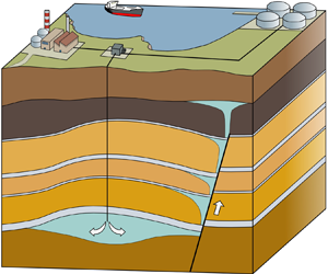
Buoyancy-driven flows in porous media have many important practical applications, linked to the movement of fluids in the subsurface. Examples include the characterisation of geothermal systems (Cheng Reference Cheng1979; Mahmoudi, Hooman & Vafai Reference Mahmoudi, Hooman and Vafai2019), predicting the movement of groundwater contaminating non-aqueous phase liquids such as chlorinated organic solvents (Taylor et al. Reference Taylor, Pennell, Abriola and Dane2001; Bear & Cheng Reference Bear and Cheng2010) and monitoring the motion and storage security of carbon dioxide (CO $_2$) linked with large-scale carbon capture and storage projects (Huppert & Neufeld Reference Huppert and Neufeld2014). The latter have recently received much attention with the growing consensus that large quantities of anthropogenic CO
 $_2$ emissions will need to be captured and stored in the subsurface to meet global emissions targets (IPCC 2018; IEA 2020).
The release of a contaminant or the injection of CO $_2$ results in fluid travelling through the reservoir as a result of gravitational forces until it reaches a confining layer. In typical CO
 $_2$ injection scenarios, the buoyant CO
 $_2$ rises until it reaches a structural seal, a low permeability rock layer such as a shale, anhydrite or salt, which prevents the fluid from migrating beyond the storage reservoir. For geological carbon storage to be successful, it is vital that the CO
 $_2$ remains securely trapped in the subsurface over long time scales (Metz et al. Reference Metz, Davidson, Coninck, Loos and Meyer2005). Defects within the seal may allow stored CO
 $_2$ to leak into overlying aquifers and eventually to the surface. Therefore, it is important to understand how these defects may contribute to the migration of CO
 $_2$. Likewise, for contaminants in the subsurface the influence of defects in the reservoir seal may impact the dispersal of the contaminant.
Faults, which are localised zones of brittle deformation, are a common feature in geological reservoirs, and may act as leakage pathways for trapped fluids. There is a large body of work on the structure and fluid flow properties of fault zones (Caine, Evans & Forster Reference Caine, Evans and Forster1996; Faulkner et al. Reference Faulkner, Jackson, Lunn, Schlische, Shipton, Wibberley and Withjack2010; Nicol et al. Reference Nicol, Seebeck, Field, McNamara, Childs, Craig and Rolland2017). A simple model for the structure of a fault zone is a fault core, generally consisting of very fine grained crushed rock (gouge) and larger fragments of broken up host rock, surrounded by a heavily fractured damage zone (Wibberley, Yielding & Toro Reference Wibberley, Yielding and Toro2008). The fault core and surrounding damage zone have very different hydraulic properties. Laboratory measurements on samples of fault core show that the permeability can be reduced by two to three orders of magnitude compared with the unfaulted host rock (Zhang & Tullis Reference Zhang and Tullis1998; Shipton et al. Reference Shipton, Evans, Robeson, Forster and Snelgrove2002; Shipton, Evans & Thompson Reference Shipton, Evans and Thompson2005). In contrast, the presence of fracture networks in the fault damage zone can increase the permeability of the host rock by two to three orders of magnitude (Simpson, Guéguen & Schneider Reference Simpson, Guéguen and Schneider2001; Oda, Takemura & Aoki Reference Oda, Takemura and Aoki2002; Mitchell & Faulkner Reference Mitchell and Faulkner2008). The resultant model for fluid flow in fault zones is a barrier-conduit system, where the fault core acts as a barrier to across-fault flow and the fracture damage zone channels flow parallel to the fault plane (Caine et al. Reference Caine, Evans and Forster1996; Balsamo et al. Reference Balsamo, Storti, Salvini, Silva and Lima2010). Studies have applied this model to explore vertical exchange flows through faults between multiple aquifers (Woods et al. Reference Woods, Hesse, Berkowitz and Chang2015) and upward migration of CO $_2$ into overlying permeable formations (Chang, Minkoff & Bryant Reference Chang, Minkoff and Bryant2008; Kang et al. Reference Kang, Nordbotten, Doster and Celia2014).
Faults are relatively small features in basin-scale models, so can be computationally challenging and expensive to model accurately using standard multi-scale numerical flow simulations (Class et al. Reference Class2009; Nordbotten et al. Reference Nordbotten, Kavetski, Celia and Bachu2009). One option is to develop analytical models that describe fault behaviour, which are then integrated into the larger-scale models (Nordbotten & Celia Reference Nordbotten and Celia2011; Kang et al. Reference Kang, Nordbotten, Doster and Celia2014). These models are constrained by the assumptions needed to solve the mathematical system of equations, but solutions can be obtained in seconds as opposed to hours/days, and developing these models also provides insight into the dominant physical processes in the system.
A number of studies have focused on analytical solutions for buoyancy-driven flows or on gravity currents in porous media with leakage from the current. This includes gravity currents in unconfined porous media leaking steadily through a permeable boundary (Acton, Huppert & Worster Reference Acton, Huppert and Worster2001; Pritchard, Woods & Hogg Reference Pritchard, Woods and Hogg2001; Pritchard & Hogg Reference Pritchard and Hogg2002), or leaking through discrete fractures, where the leakage flux is driven by the hydrostatic pressure of the underlying less dense fluid (Pritchard Reference Pritchard2007) or with the added effect of the buoyancy of fluid in the fault (Neufeld, Vella & Huppert Reference Neufeld, Vella and Huppert2009). Previous studies have also considered leakage in confined aquifers (Avci Reference Avci1994; Nordbotten, Celia & Bachu Reference Nordbotten, Celia and Bachu2004, Reference Nordbotten, Celia and Bachu2005) where leakage is driven by an increased pressure due to injection or where a background pressure gradient between multiple aquifers contributes to driving leakage through fractures (Pegler, Huppert & Neufeld Reference Pegler, Huppert and Neufeld2014b). In all of these studies, the leakage flux is driven by the Darcy velocity in the leaking boundary or fracture, which is a product of the mobility of the injected fluid in the layer or fracture and the pressure gradient across it.
The movement of fluids through porous rocks and small-scale fractures can be modelled by considering miscible flows in porous media, where the flow is governed by Darcy's law. Miscible flows in porous media can be characterised by their Péclet number,  ${\textit {Pe}} = d_0U\tau / D_d$, which describes the relative importance of advection to diffusion in fluid transport. Here,
  $d_0$ is the mean grain diameter,
  $U$ is the characteristic velocity of the flow,
  $\tau$ is the tortuosity of the porous medium and
  $D_d$ is the molecular diffusion coefficient. A composite transport coefficient
  $D$ can model the diffusive and dispersive contributions to movement of fluid, where
 \begin{equation} D = d_0 U \left( 1+ \frac{1}{{\textit{Pe}}}\right) \end{equation}
(Houseworth Reference Houseworth1984; Delgado Reference Delgado2007). In diffusion dominated flows, where  ${\textit {Pe}} \ll 1$, the transport coefficient
  $D\simeq D_d/\tau$ is constant whereas in advection dominated flows, where
  ${\textit {Pe}} \gg 1$,
  $D\simeq d_0U$ is dependent on the flow speed.
As a buoyant fluid is injected into a reservoir or escapes through a fracture into an adjacent aquifer, it initially forms a buoyant plume. The behaviour of a buoyant plume in porous media was first studied by Wooding (Reference Wooding1963), who mathematically modelled the dynamics of a rectilinear plume in porous media for Darcy flow. He derived a similarity solution that predicts the amount of entrainment from the ambient and therefore describes the increasing volume flux of the plume with height. Sahu & Flynn (Reference Sahu and Flynn2015) derived a new similarity solution for Darcy plumes with large Péclet numbers to obtain expressions for the plume volume flux and mean reduced gravity as functions of vertical distance from the source.
In this study we develop an analytical model to describe the dynamics of leakage through a fault zone cutting multiple aquifers and seals, which we test against a new set of laboratory experiments. To model flow in faults cross-cutting multiple aquifers, we combine current analytical models for a buoyant plume in a semi-infinite porous medium (Sahu & Flynn Reference Sahu and Flynn2015) and a leaking gravity current (Pritchard Reference Pritchard2007; Neufeld et al. Reference Neufeld, Vella and Huppert2009) with a new model for fault leakage which accounts for increased pressure gradients within the fault due to an increase in Darcy velocity directly above the fault. Previous studies providing analytical solutions to fault leakage problems have used numerical solvers to verify their models (Kang et al. Reference Kang, Nordbotten, Doster and Celia2014). Here, we test the results with a novel set of porous media tank experiments which show a good fit to the model. The results of the modelling are illustrated by application to a naturally occurring CO $_2$-charged aquifer system at Green River, Utah, using an extension of the model to calculate the fluid distribution across multiple vertically stacked aquifers, cross-cut by a fault.
In § 2 we formulate a theoretical model for the half-space plume in which the plume volume flux and mean reduced gravity are used as inputs in a model for a leaking gravity current and where leakage through the fault is driven by the hydrostatic pressure within the underlying gravity current and the buoyancy of the fluid in the fault. In § 3 we show numerical results for the gravity current shape and leakage rates. Observations from experiments show that an increase in Darcy velocity within the secondary plume above the fault leads to enhanced pressure gradients within the fault. In § 4 an expression for the pressure above the fault is coupled with the leakage model presented in § 2, resulting in a new model for leakage through the fault. The model is matched against results from a set of analogue porous medium tank experiment in § 5, and in § 6 we demonstrate the application of the model in CO $_2$ storage by applying an extension of the model to predict CO
 $_2$ leakage across multiple aquifers. In § 7 we consider the validity of our model and discuss potential limitations and extensions including the explicit inclusion of multiphase flow relationships in the plume, gravity current and fault leakage models. Finally, we present the conclusions from this study in § 8.
2. Theoretical model
In this section, we present a model for calculating the leakage flux from an aquifer intersected by a fault. To achieve this, we couple a model for a buoyant plume in a semi-infinite porous medium with a model for a two-dimensional gravity current spreading under an impermeable base containing a fault of finite gap width and thickness, and known permeability and porosity.
2.1. Buoyant plume in a semi-infinite porous aquifer
Here, we derive a solution for the steady flow of a two-dimensional buoyant plume in a semi-infinite porous medium with unit thickness in the third dimension. A constant input flux  $q_0$ of fluid with density
  $\rho _0$ is injected into a porous medium with permeability
  $k$ and porosity
  $\phi$ saturated with a denser ambient fluid of density
  $\rho _a$. Both fluids are assumed to be miscible, with equal viscosities such that there are no capillary effects during the flow. The implications of this assumption for application to CO
 $_2$–water systems is discussed in § 7. The injected fluid mixes with the ambient fluid and forms a plume with a volume flux
  $Q(z)$ and density
  $\rho (x,z)$ at a given height
  $z$ (figure 1a). We follow the analysis of Sahu & Flynn (Reference Sahu and Flynn2015) who considered an unconfined plume in a porous medium for Darcy flow with
  ${\textit {Pe}} \gg 1$, in contrast to Wooding (Reference Wooding1963). Our analysis differs by considering a half-space model, with an impermeable vertical boundary contacting the injection location. Assuming steady Boussinesq flow (shown in previous studies to be a useful approximation in CO
 $_2$–water systems (Soltanian et al. Reference Soltanian, Amooie, Dai, Cole and Moortgat2016; Amooie, Soltanian & Moortgat Reference Amooie, Soltanian and Moortgat2018)), the governing equations based on mass continuity, momentum continuity, solute transport and a linear equation of state are
 \begin{gather} \frac{\partial u}{\partial x} + \frac{\partial w}{\partial z} = 0, \end{gather}
 \begin{gather}\frac{1}{\rho_a}\frac{\partial P}{\partial x} + \frac{\nu}{k}u = 0, \end{gather}
 \begin{gather}\frac{1}{\rho_a}\frac{\partial P}{\partial z} + \frac{\nu}{k}w ={-}\frac{g\rho}{\rho_a}, \end{gather}
 \begin{gather}\frac{1}{\phi}\left( w \frac{\partial C}{\partial z} + u\frac{\partial C}{\partial x} \right) = \frac{\partial }{\partial x}\left(D_T \frac{\partial C}{\partial x}\right) + \frac{\partial }{\partial z}\left(D_L\frac{\partial C}{\partial z}\right), \end{gather}
 \begin{gather}\rho = \rho_a (1 - \beta C), \end{gather}
where  $u$ and
  $w$ are the fluid velocities in the
  $x$ and
  $z$ directions respectively,
  $P$ is the fluid pressure,
  $\nu$ is the kinematic viscosity,
  $g$ is the acceleration due to gravity,
  $C$ is the solute concentration,
  $\beta$ is the solutal expansion coefficient and
  $D_L$ and
  $D_T$ are the longitudinal and transverse dispersion coefficients, respectively. Since the plume is long and thin we may neglect vertical variations in the horizontal velocity
  $({\partial w}/{\partial x} \gg {\partial u}/{\partial z})$ and longitudinal dispersion. Hence, the combined momentum equations and the solute transport equation become,
 \begin{gather} \frac{\nu}{k}\frac{\partial w}{\partial x} ={-}\frac{g}{\rho_a}\frac{\partial \rho}{\partial x}, \end{gather}
 \begin{gather}u\frac{\partial C}{\partial x} + w \frac{\partial C}{\partial z} = \phi \frac{\partial }{\partial x}\left(D_T\frac{\partial C}{\partial x}\right). \end{gather}
We now introduce a streamfunction  $\psi$ such that
  $w = {\partial \psi }/{\partial x}$ and
  $u = -({\partial \psi }/{\partial z})$. For
  ${\textit {Pe}} \gg 1$, the transverse dispersion coefficient may be approximated as
 \begin{equation} D_T \simeq \alpha w, \end{equation}
where  $\alpha$ is the transverse dispersivity (Delgado Reference Delgado2007). On using (2.5) and (2.8), (2.6) and (2.7) become
 \begin{gather} \frac{\partial^{2} \psi}{\partial x^{2}} = \frac{g\beta k}{\nu}\frac{\partial C}{\partial x}, \end{gather}
 \begin{gather}\frac{\partial \psi}{\partial x}\frac{\partial C}{\partial z} - \frac{\partial \psi}{\partial z}\frac{\partial C}{\partial x} = \phi\alpha\left( \frac{\partial^{2} \psi}{\partial x^{2}}\frac{\partial C}{\partial x} + \frac{\partial \psi}{\partial x}\frac{\partial^{2} C}{\partial x^{2}}\right). \end{gather}
For a steady plume, the buoyancy flux, or equivalently the solute mass flux, remains constant with height, as the horizontally entraining ambient fluid only increases the volume of the plume but does not alter the solute mass. The buoyancy flux of the plume per unit thickness is conserved with height and is
 \begin{equation} F_0 = \int_{0}^{\infty}w g'\,{\textrm{d}\kern0.06em x}, \end{equation}
where  $g' = g(\rho _a -\rho )/\rho _a \equiv g\beta C$ is the reduced gravity. A scaling analysis of (2.9), (2.10) and (2.11) suggests that
 \begin{gather} \frac{\psi}{x^{2}} \sim \frac{g\beta k}{\nu}\frac{C}{x}, \end{gather}
 \begin{gather}\frac{\psi C}{xz} \sim \phi \alpha \frac{\psi C}{x^{3}}, \end{gather}
 \begin{gather}F_0 \sim wg'x \sim \psi g\beta C. \end{gather}
Equation (2.12b) motivates us to define a self-similar horizontal length scale of the plume
 \begin{equation} \eta = \frac{x}{\sqrt{\phi\alpha z}} \quad (z > 0), \end{equation}
where we note that  $z=0$ is the point of injection and therefore entrainment of the ambient fluid and the corresponding plume equations are applicable only for
  $z>0$. It is also worth noting that the plume is defined as the region of the flow field where the concentration
  $C>0$, or equivalently
  $g'>0$. Now, on considering (2.12a), (2.12c) and (2.13) together, we can define the streamfunction and concentration of the plume in the forms of similarity functions
  $\mathscr {F}(\eta )$ and
  $\mathscr {G}(\eta )$ as
 \begin{equation} \psi = \left[\left(\frac{F_0 k}{ \nu}\right)^{2} \phi\alpha z \right]^{1/4} \mathscr{F}(\eta), \end{equation}
and
 \begin{equation} C = \frac{1}{g\beta} \left[\left(\frac{F_0\nu}{ k}\right)^{2} \frac{1}{\phi\alpha z} \right]^{1/4} \mathscr{G}(\eta), \end{equation}
respectively. These expressions for  $\psi$ and
  $C$ are related by (2.9) such that
  $\mathscr {F'}(\eta ) = \mathscr {G}(\eta )$. Similarly solute concentration, (2.10) implies that
 \begin{equation} \mathscr{F'''}\mathscr{F'}+ \mathscr{F''}\mathscr{F''}+ \tfrac{1}{4}\mathscr{F''}\mathscr{F}+ \tfrac{1}{4}\mathscr{F'}\mathscr{F'}= (\mathscr{F''}\mathscr{F'})' + \tfrac{1}{4}(\mathscr{F'}\mathscr{F})' = 0. \end{equation}
We solve (2.16) subject to the conditions that the solute concentration cannot be negative, and tends to the background concentration in the far field,  $C(x,z) = 0$ and
  $\mathscr {F'}(\eta )=0$ as
  $x,\eta \to \infty$, whereas inside the plume
  $C(x,z)>0$ and
  $\mathscr {F'}(\eta ) > 0$. The transverse velocity against the fault is zero, such that the value of the streamfunction
  $\psi (0,z) = 0$ so
  $\mathscr {F}(0) = 0$. With these conditions, it can be shown that
 \begin{equation} \mathscr{F}(\eta)=\begin{cases} c \sin{\dfrac{\eta}{2}},& \eta < {\rm \pi},\\ c, & \eta > {\rm \pi}, \end{cases}\quad \text{and}\quad \mathscr{G}(\eta)= \mathscr{F'}(\eta)= \begin{cases} \dfrac{c}{2} \cos{\dfrac{\eta}{2}},& \eta < {\rm \pi},\\ 0, & \eta > {\rm \pi}, \end{cases} \end{equation}
where  $c=\sqrt {8/{\rm \pi} }$ is a constant of integration which is obtained by applying the solutions for
  $w$
$w$  $(= {\partial \psi }/{\partial x})$ and
  $g'$ (
 $=g\beta C$) to (2.11). Therefore, the expression for the volume flux per unit thickness of the plume is
 \begin{equation} Q = \int_{0}^{\infty} w\,{\textrm{d}\kern0.06em x} = \left[\left( \frac{8 F_0k}{\nu{\rm \pi}} \right)^{2} \phi\alpha z\right]^{1/4}. \end{equation}
This result is a factor of  $\sqrt {2}$ smaller than the volume flux of the unconfined plume given by Sahu & Flynn (Reference Sahu and Flynn2015). Using (2.18), the average reduced gravity across the plume can be calculated as a function of height,
 \begin{equation} \bar{g'} = \frac{F_0}{Q} = \left[\left( \frac{{\rm \pi} F_0\nu}{8 k} \right)^{2} \frac{1}{\phi\alpha z}\right]^{1/4}. \end{equation}
The equations here are for an ideal plume formed purely by a buoyancy flux, where the volume flux  $Q \to 0$ as
  $z \to 0$. For a non-ideal plume with a finite volume flux these assumptions do not hold. We can correct for this by extrapolating the flow to negative values of
  $z$ and defining a point
  $z = -z_0$ where the plume flux
  $Q(-z_0)=0$. The virtual source location
  $z_0$ is given by
 \begin{equation} z_0 = \frac{1}{\phi\alpha}\left(\frac{{\rm \pi}\nu}{8F_0k }\right)^{2} q_0^{4}, \end{equation}
where  $q_0$ is the volume flux into the system, and the buoyancy flux
  $F_0 = q_0 g'_0$ where
  $g'_0$ is the reduced gravity of the injected fluid. Given these corrections for source conditions, expressions for the plume volume flux per unit thickness and mean reduced gravity are
 \begin{equation} Q = \left[\left(\frac{8 q_0g'_0k }{\nu{\rm \pi}} \right)^{2} \phi\alpha(z+z_0)\right]^{1/4}, \end{equation}
and
 \begin{equation} \bar{g'} = \left[\left( \frac{{\rm \pi} q_0g'_0\nu}{8 k } \right)^{2} \frac{1}{\phi\alpha (z+z_0)}\right]^{1/4} . \end{equation}
Figure 1. (a) Fluid with density  $\rho _0$ is injected with a constant input flux
  $q_0$ into a porous medium with permeability
  $k$ and porosity
  $\phi$, saturated with an ambient fluid of density
  $\rho _a$. The fluid forms a plume with a volume flux
  $Q(z)$ and density
  $\rho (x,z)$ at a given height
  $z$. (b) After the buoyant plume reaches the top of the aquifer, it provides a constant input flux
  $q$ of fluid with density
  $\rho _1$ into a gravity current which spreads into a porous medium of permeability
  $k$ and porosity
  $\phi$ saturated with an ambient fluid of density
  $\rho _a$. The thickness of the current is given by
  $h(x,t)$. The current spreads under an impermeable baffle containing a fault of gap width
  $d_f$, thickness
  $h_f$, permeability
  $k_f$ and porosity
  $\phi _f$ between
  $x=0$ and
  $x=d_f$. Injected fluid leaks through the fault with flux
  $q_F$.
2.2. Gravity current with leaking fault at the origin
Here, we consider the behaviour of a two-dimensional density-driven flow of a fluid in a porous medium of permeability  $k$ and porosity
  $\phi$ saturated with an ambient fluid of higher density
  $\rho _a$ and bounded on one side by an impermeable vertical boundary (figure 1b). The injected fluid spreads below an impermeable horizontal baffle containing a fault of gap width
  $d_f$, thickness
  $h_f$, permeability
  $k_f$ and porosity
  $\phi _f$ which abuts the boundary. At the horizontal baffle, a gravity current forms due to fluid input from a rising plume. The fluid density
  $\rho _1$ and input rate
  $q$ into the gravity current are calculated using the expressions for the plume volume flux and mean reduced gravity derived in (2.21) and (2.22). The values of
  $q$ and
  $\bar {g'}$ are evaluated at a vertical distance
  $H$ from the initial injection point, which corresponds with the level of the base of the impermeable baffle. We assume that the depth of the ambient fluid is large compared with the thickness of the current
  $(H\gg h)$. This means we can neglect the effects of flow in the ambient and assume the values of
  $q$ and
  $\bar {g'}$ remain constant with time.
Using (2.21) and (2.22), we obtain expressions for the input flux into the current and reduced gravity of the current,
 \begin{equation} q = \left[\left( \frac{8q_0g'_0k}{\nu{\rm \pi}} \right)^{2} \phi\alpha H(1+\theta)\right]^{1/4} \quad \mathrm{and} \quad g' = \left[\left( \frac{{\rm \pi} q_0g'_0\nu}{8k} \right)^{2} \frac{1}{\phi\alpha H (1 + \theta)}\right]^{1/4}, \end{equation}
where the dimensionless parameter
 \begin{equation} \theta = \frac{z_0}{H} = \frac{1}{\phi \alpha H}\left(\frac{{\rm \pi}\nu q_0}{8g'_0k}\right)^{2}. \end{equation}
At the impermeable baffle, the injected fluid forms a gravity current, with some fluid leaking through the fault. We assume that the current is long and thin, and the velocity is predominantly parallel to the baffle so that the pressure in the current is hydrostatic. The fault is modelled using the barrier-conduit system described in § 1, with the fault damage zone within the baffle modelled using an average permeability  $k_f$ and width
  $d_f$. Neufeld et al. (Reference Neufeld, Vella and Huppert2009) formulated a model for drainage through a fissure of given permeability and width, which incorporates both flow driven by hydrostatic pressure as well as the buoyancy of the fluid in the fault itself,
 \begin{equation} w_f(t) = \frac{k_f}{\mu}\frac{{\rm \Delta} \rho g (h_0(t) + h_f)}{h_f} = \frac{k_f g' h_0(t)}{\nu h_f}\left[1+\frac{h_f}{h_0(t)}\right]. \end{equation}
Here,  $k_f$ is the permeability of the fault,
  $h_f$ is the length of the fault,
  $\mu$ is the dynamic viscosity and
  $\nu$ is the kinematic viscosity of the leaking fluid,
  $h_0$ is the thickness of the current at
  $x=0$
$x=0$  $(h_0 = h(0,t))$ and
  $g'$ is the reduced gravity of the current. Note that, despite the width of the fault,
  $d_f>0$, we assume that its effect on the gravity current is localised to the point
  $x = 0$, and the leakage is driven by the thickness there. A sharp interface between the injected and ambient fluids is described by a thickness
  $h(x,t)$ below the baffle at
  $z = H$. Dispersion will occur predominantly at the edges of the gravity current as it propagates into the reservoir and is expected to alter the shape of the current, the implications of which are discussed during comparison with the experimental results in § 5.3. However, where the plume feeds the current directly below the fault, dispersion will be less pronounced. Hence, we neglect dispersion in the gravity current as it does not significantly affect leakage through the fault. The flow in the gravity current is driven by gradients in the hydrostatic pressure, and the evolution of the height is determined by the divergence of the fluid flux,
 \begin{equation} \phi \frac{\partial h}{\partial t} = \frac{kg'}{\nu}\frac{\partial }{\partial x} \left(h\frac{\partial h}{\partial x}\right). \end{equation}
The current forms when the plume impacts the impermeable baffle, and has initial condition
 \begin{equation} h(x,0) = 0. \end{equation}
Subsequently the gravity current is fed by the plume and has boundary conditions,
 $$\begin{gather} \left[\frac{kg'}{\nu}h\frac{\partial h}{\partial x}\right]_{x=0} ={-}(q - q_F), \quad \left[\frac{kg'}{\nu}h\frac{\partial h}{\partial x}\right]_{x=x_N} = 0, \quad h(x_N,t) = 0, \end{gather}$$
which describe the input flux at the origin (equal to the plume input flux  $q$, minus the fault leakage flux
  $q_F$), a no flux condition through the nose of the current and zero thickness at the nose of the current. The current satisfies global conservation of mass given by,
 \begin{equation} \phi \int_0^{x_N} h\,{\textrm{d}\kern0.06em x} = q t - \frac{d_f \phi_f k_f g'}{\nu h_f} \int_0^{t} h_0\left( 1 + \frac{h_f}{h_0} \right){\textrm{d}}t, \end{equation}
where the final term comes from (2.25) and is equal to the total volume of fluid that has leaked through the fault. Note that time  $t=0$ in (2.29) is the instance the plume first reaches the impermeable baffle at
  $z=H$.
2.2.1. Non-dimensionalisation
Based on (2.23a,b), (2.26) and (2.29) we define the following dimensionless variables,
 \begin{gather} \tilde{x} = \frac{g' k_f^{2}d_f^{2}\phi_f^{2}}{kq\nu h_f^{2}}x = \frac{{\rm \pi} k_f^{2} d_f^{2} \phi_f^{2}}{8 k^{2}h_f^{2}\phi^{1/2}\alpha^{1/2} H^{1/2}(1+\theta)^{1/2}}x, \end{gather}
 \begin{gather}\tilde{h} = \frac{g' k_f d_f\phi_f}{q\nu h_f}h = \frac{{\rm \pi} k_f d_f \phi_f}{8 k h_f \phi^{1/2}\alpha^{1/2} H^{1/2}(1+\theta)^{1/2}} h, \end{gather}
 \begin{gather}\tilde{t} = \frac{ g'^{2} k_f^{3} d_f^{3} \phi_f^{3}}{k\phi q\nu^{2} h_f^{3}} t = \frac{{\rm \pi}^{3/2}k_f^{3} d_f^{3}\phi_f^{3}q_0^{1/2}g_0^{\prime 1/2}}{8^{3/2}k^{5/2}h_f^{3}\nu^{1/2} \phi^{7/4}\alpha^{3/4} H^{3/4}(1+\theta)^{3/4}} t. \end{gather}
By substituting (2.30a–c), (2.26)–(2.29) become,
 \begin{gather} \frac{\partial \tilde{h}}{\partial \tilde{t}} = \frac{\partial }{\partial \tilde{x}} \left(\tilde{h}\frac{\partial \tilde{h}}{\partial \tilde{x}}\right), \end{gather}
 \begin{gather}\tilde{h}(\tilde{x},0) = 0 \quad \mathrm{and} \quad \tilde{h}(\widetilde{x_N},\tilde{t}) = 0, \end{gather}
 \begin{gather}\int_0^{\tilde{x}_N} \tilde{h}\,{\textrm{d}\kern0.06em }\tilde{x} = \tilde{t} -\int_0^{\tilde{t}} \tilde{h}_0 \left( 1+ \frac{h_f}{\tilde{h}_0}\frac{k_f d_f \phi_f g'}{q \nu h_f}\right) {\textrm{d}}\tilde{t}. \end{gather}
We introduce the dimensionless parameter
 \begin{equation} \lambda = \frac{g' k_f d_f \phi_f}{q\nu} = \frac{{\rm \pi} k_f d_f \phi_f}{8 k \phi^{1/2} \alpha^{1/2} H^{1/2} (1+\theta)^{1/2}}, \end{equation}
that characterises the strength of leakage through the fault due to the buoyancy of fluid in the fault so that (2.33) now has the form,
 \begin{equation} \int_0^{\tilde{x}_N} \tilde{h}\,{\textrm{d}}\kern0.06em \tilde{x} = (1-\lambda)\tilde{t} -\int_0^{\tilde{t}} \tilde{h}_0 \,{\textrm{d}}\tilde{t}. \end{equation}
Here,  $\lambda =0$ describes the case where the leakage through the fault is only driven by the hydrostatic pressure within the underlying gravity current, and not by the buoyancy of fluid in the fault.
3. Numerical solutions
We solve for the full time-dependent behaviour of the gravity current numerically using a finite difference scheme. The thickness profile of the current is initially  $\tilde {h}(\tilde {x},0) = 0$, and the subsequent evolution is described by (2.31)–(2.35). The thickness at
  $\tilde {x}=0$ is obtained by solving (2.35) at each time step, using the thickness profile obtained from solving (2.31) and calculating the new leaked volume of fluid using
  $\tilde {h}_0$ from the previous time step. Results obtained are shown in figures 2–4.

Figure 2. (a) Thickness profiles of the gravity current from  $\tilde {t}=5$ to
  $\tilde {t}=50$ at intervals of 5 for the
  $\lambda = 0$ case. (b) Normalised thickness profiles for
  $\lambda = 0$ showing the change in shape of the current over time and deviation away from the self-similar zero leakage solution.
Figure 2(a) illustrates the solution for the gravity current shape as a function of time. The thickness profiles of the current are plotted from  $\tilde {t}=0$ to
  $\tilde {t}=50$ at intervals of 5 with
  $\lambda =0$, which describes the case where leakage through the fault is only driven by the hydrostatic pressure within the current below the fault. Figure 2(b) shows three height profiles at
  $\tilde {t}=0.5$,
  $\tilde {t}=5$ and
  $\tilde {t}=50$ (solid lines), where the extent and height of the profiles have been normalised by the maximum extent
  $\tilde {x}_N$ and the thickness of the current at
  $\tilde {x}=0$,
  $\tilde {h}_0$. The self-similar solution for the propagation of a gravity current through a porous medium with a constant input flux and with zero leakage (Huppert & Woods Reference Huppert and Woods1995) is also plotted (dashed line). The solutions for the leaking gravity current deviate from the zero leakage case over time, demonstrating a non-self-similar behaviour of the leaking current.
In figure 3(a), the evolution of the horizontal and vertical extent of the leaking gravity current is plotted for  $\lambda =0$ (solid lines). At early times, the horizontal extent evolves following a
  $\tilde {t}^{2/3}$ power law relationship and the vertical extent of the current evolves following a
  $\tilde {t}^{1/3}$ power law relationship which agrees with the solutions for a gravity current with no leakage (Huppert & Woods Reference Huppert and Woods1995). At late times, the horizontal and vertical extent evolution deviate from these power law relationships. The vertical extent of the current tends to a constant value, resulting in a constant rate of leakage from the current. Late time asymptotic behaviour of (2.28) and (2.29) indicates that the thickness at the origin
  $h_0$ asymptotes to a constant as the gravity current nose tends towards infinity. It is possible to show (by considering a small perturbation to this equilibrium point) that the nose position approaches infinity like
  $x_N \sim (qt)^{1/2}$ in this late time regime (see Appendix A). This late time behaviour can be seen if the gradients of the log–log graph for the vertical and horizontal extent of the current are plotted as a function of time (figure 3b).

Figure 3. (a) Leaking gravity current horizontal extent and vertical extent at  $\tilde {x}=0$ plotted as a function of
  $\tilde {t}$ for the
  $\lambda = 0$ case (solid lines). Dashed lines show the power law behaviour of a gravity current with no leakage. (b) Gradient of the logarithmic horizontal and vertical extent evolution plotted as a function of time (solid lines). The horizontal and vertical extent deviate away from the 2/3 and 1/3 power law relationships of a gravity current with no leakage (dashed lines).
The total injected volume of fluid into the system increases linearly with time and partitions between the gravity current and any leaked volume through the fault. A quantitative understanding of this partitioning is a key metric for the storage security of injected fluids in the subsurface. The total injection volume, gravity current volume and total leaked volume, represented by the terms  $\tilde {t}$,
  $\int _0^{\tilde {x}_N} \tilde {h}\,{\textrm {d}}\tilde {x}$ and
  $\int _0^{\tilde {t}} (\tilde {h}_0 + \lambda )\,{\textrm {d}}\tilde {t}$ in (2.35), are calculated as a function of time and plotted in figure 4(a) for different values of
  $\lambda$.

Figure 4. (a) Total injection volume, gravity current volume and total leaked volume plotted as a function of time for  $\lambda = 0$, 0.1, 0.2 and 0.3. (b) Injection rate, rate of fluid input into the gravity current and the rate of leakage through the fault as a function of time.
Initially, the volume of fluid going into the gravity current is greater than the volume of the fluid leaking through the fault. However, as the height of the current below the fault increases, a larger hydrostatic pressure drives more fluid through the fault and the volume of fluid leaking becomes larger than the volume of fluid going into the gravity current. This transition can be seen when the fluxes of fluid going into the gravity current and leaking through the fault are plotted as a function of time (figure 4b). The value of  $\lambda$ signifies the buoyancy of fluid in the fault. As
  $\lambda$ increases, the buoyancy flux through the fault increases, and so the leakage flux is a larger proportion of the total flux into the system.
4. A simple model for the pressure above the baffle
The theoretical model described in § 2 accounts for leakage due to the hydrostatic pressure in the underlying gravity current and the buoyancy of the fluid in the fault. In several of our laboratory experiments (presented in § 5), we observe a thinning of the secondary plume that forms above the baffle close to the fault (figure 5c). The thinning may be caused by an acceleration of the secondary plume, leading to differential negative pressures near the fault which increase the total pressure gradient across the fault. Transport of concentration in the secondary plume is similar to that described in § 2.1, but the length scale over which this dispersion plays an important role is much larger than the length scale for the thinning of the plume (figure 11b), hence we do not include these effects. In this section we create a model for the pressure above the baffle by considering an asymptotic expansion in terms of a small deviation to the plume inlet velocity.

Figure 5. (a) Schematic diagram illustrating the different parameters of the problem. The secondary plume  $z\geq 0$ is fed by a pressure-driven flow
  $w_f$ through the fault, but must accelerate to match the natural buoyancy velocity
  $w_b$ downstream. Hence, the plume width
  $d(z)$ thins out from initial width
  $d_f$ to ultimate width
  $d_b$, resulting in a differential negative pressure
  $p^{-}$ near its source. Note the redefined position of
  $z=0$. (b) Figurative plot of the vertical pressure profile above the fault. (c) Close up of a laboratory experiment showing thinning of the secondary plume above the baffle (note orientation of experimental image has been rotated by
  $180^{\circ }$, see § 5).
4.1. Thinning plume model
The scenario we consider is illustrated in figure 5(a). Note the redefined position of  $z=0$. The secondary plume
  $z\geq 0$ is fed by a vertical inlet velocity
  $w_f$ which is slightly smaller than the buoyancy velocity
  $w_b=k{\rm \Delta} \rho g/\mu$, such that
  $w_f=w_b(1-\epsilon )$ for some small parameter
  $\epsilon \ll 1$. As a result, the width of the plume, which we denote
  $d(z)$, must reduce from an initial value
  $d_f$ to a far-field value
  $d_b=w_f d_f/w_b$. Note that it is possible for
  $\epsilon$ to be negative, in which case the width of the secondary plume would increase. We model the flow into the secondary plume using Darcy's law and mass conservation,
 \begin{equation} \boldsymbol{u}={-}\frac{k}{\mu} \boldsymbol{\nabla} \left( p + \rho_1 g z \right),\quad \boldsymbol{\nabla} \boldsymbol{\cdot} \boldsymbol{u}=0, \end{equation}
along with boundary conditions corresponding to constant inflow across the fault, impermeability at the vertical left-hand wall and far-field velocity conditions
 \begin{gather} w=w_b(1-\epsilon),\quad \mathrm{at}\ z=0, \end{gather}
 \begin{gather}u=0,\quad \mathrm{at}\ x=0, \end{gather}
 \begin{gather}w\rightarrow w_b,\quad \mathrm{at}\ z\rightarrow \infty, \end{gather}
respectively, where  $u$ and
  $w$ are the fluid velocities in the
  $x$ and
  $z$ directions. At the edge of the steady plume, we impose a kinematic boundary condition and we enforce that the pressure equals the ambient hydrostatic
 \begin{equation} u=w\frac{\mathrm{d} d}{\mathrm{d}z},\quad \mathrm{and} \quad p=p_a-\rho_a g z, \quad \mathrm{at}\ x=d(z). \end{equation}
The pressure at the edge of the plume is hydrostatic (4.5), since it must match with the pressure in the adjacent static ambient fluid. We therefore consider an asymptotic solution of the form
 \begin{gather} u=\epsilon \hat{u}(x,z)+\cdots, \end{gather}
 \begin{gather}w=w_b+\epsilon \hat{w}(x,z)+\cdots, \end{gather}
 \begin{gather}p=p_a-\rho_a g z+\epsilon \hat{p}(x,z)+\cdots, \end{gather}
 \begin{gather}d=d_f+\epsilon \hat{d}(z)+\cdots, \end{gather}
for  $\epsilon \ll 1$. Clearly in the limit
  $\epsilon \rightarrow 0$ the leading-order terms in (4.6)–(4.9) satisfy (4.1)–(4.5), as expected. At first order in
  $\epsilon$, the pressure must satisfy the linear system
 \begin{gather} \nabla^{2} \hat{p}=0, \end{gather}
 \begin{gather}\frac{\partial \hat{p}}{\partial z}={\rm \Delta} \rho g,\quad \mathrm{at}\ z=0, \end{gather}
 \begin{gather}\frac{\partial \hat{p}}{\partial x}=0,\quad \mathrm{at}\ x=0, \end{gather}
 \begin{gather}\frac{\partial \hat{p}}{\partial z}\rightarrow 0,\quad \mathrm{at}\ z\rightarrow \infty, \end{gather}
 \begin{gather}\hat{p}=0,\quad \mathrm{at}\ x=d_f, \end{gather}
 \begin{gather}\frac{\partial \hat{p}}{\partial x}={-}{\rm \Delta} \rho g \frac{\mathrm{d}\hat{d}}{\mathrm{d}z},\quad \mathrm{at}\ x=d_f. \end{gather}
Conservation of mass dictates that the pressure must satisfy Laplace's equation, which since it is linear results in (4.10). Likewise, the boundary conditions (4.2)–(4.4) and the hydrostatic condition in (4.5b) are all linear equations. Hence, they must apply to leading- and first-order pressure terms alike. The leading-order pressure solution (first part of (4.8)) satisfies all of these trivially. The only nonlinear equation is (4.5a), also known as the kinematic condition. In this case, one must expand out the variables, keeping only first-order terms, which gives (4.15). Conveniently, (4.10)–(4.14) can be solved independently of (4.15), indicating that the plume shape and the pressure are decoupled. The pressure solution is calculated by separation of variables, giving
 \begin{equation} \hat{p}={-}\frac{8{\rm \Delta} \rho g d_f}{{\rm \pi}^{2}}\sum_{n=0}^{\infty} \frac{({-}1)^{n}}{\left( 2n+1\right)^{2}} \cos\left[\left( 2n+1\right) \frac{{\rm \pi} x}{2d_f}\right]\exp({-\left( 2n+1\right){{\rm \pi} z}/{2d_f}}). \end{equation}
Hence, the pressure (including both leading- and first-order terms) at  $x=z=0$, which we denote
  $p^{-}$, is given by
 \begin{equation} p^{-}= p_a- {\rm \Delta} \rho g d_f \left[ \frac{8G}{{\rm \pi}^{2}} \left( 1-\frac{w_f}{w_b} \right) \right], \end{equation}
where  $G=\sum _{n=0}^{\infty } (-1)^{n}/(2n+1)^{2}\approx 0.9160$ is Catalan's constant. The plume shape is calculated by evaluating (4.15) and (4.16), which converges to the differential equation
 \begin{equation} \frac{\mathrm{d}\hat{d}}{\mathrm{d}z}={-}\frac{4}{\rm \pi}\tanh^{{-}1}\left[ \exp({-{\rm \pi} z/2 d_f}) \right].\end{equation}
We solve (4.18) with boundary condition  $\hat {d}(0)=0$ and plot the solution in figure 6(a). Clearly,
  $\hat {d}\rightarrow -d_f$ as
  $z\rightarrow \infty$, such that the the total plume shape
  $d_f+\epsilon \hat {d}$ asymptotes to the far-field plume width
  $d_b=d_f w_f/w_b$, as required.

Figure 6. (a) Perturbation of the width of the secondary plume (4.18). (b,c) Contour plots of the pressure above the baffle  $p^{-}$ (4.17), normalised to give a dimensionless value
  $(p^{-}-p_a)/{\rm \Delta} \rho g d_f$, for the different parameters of the problem
  $\tilde {h}_0=h_0/d_f$,
  $\tilde {h}_f=h_f/d_f$ and
  $\tilde {k}=k/k_f$. Regions of the contour plots resulting in a widening plume
  $w_f/w_b>1$ and positive values of
  $p^{-}$ are omitted.
We note that both the pressure  $p^{-}$ and the inlet velocity
  $w_f$ are unknown in (4.17). Hence, to close the system we require a second equation relating these two quantities. This is given by considering the flow through the fault
  $-h_f< z\leq 0$. In particular, as illustrated in figure 5, the flow through the fault is driven by a difference in pressure
  $p^{+}-p^{-}$, where
  $p^{+}$ is set by the thickness of the gravity current
 \begin{equation} p^{+}=p_a + {\rm \Delta} \rho g h_0 + \rho_a g h_f. \end{equation}
Hence, by approximating Darcy's law across the fault we arrive at a second relationship,
 \begin{equation} w_f={-}\frac{k_f}{\mu}\left[\frac{p^{-}-p^{+}}{h_f}-\rho_1 g\right].\end{equation}
Rearranging (4.17) and (4.20), we arrive at dimensionless equations for  $w_f/w_b$ and
  $p^{-}$,
 \begin{gather} \frac{w_f}{w_b}=\frac{1+( \tilde{h}_f+\tilde{h}_0 ){\rm \pi}^{2}/8G}{1+\tilde{k}\tilde{h}_f{\rm \pi}^{2}/8G}, \end{gather}
 \begin{gather}p^{-}= p_a- {\rm \Delta} \rho g d_f \left[\frac{\tilde{h}_f(\tilde{k}-1)-\tilde{h}_0 }{1+\tilde{k}\tilde{h}_f{\rm \pi}^{2}/8G}\right], \end{gather}
where  $\tilde {h}_0=h_0/d_f$,
  $\tilde {h}_f=h_f/d_f$ and
  $\tilde {k}=k/k_f$ are known parameters. From (4.21) and (4.22) it is clear that negative values of
  $p^{-} - p_a$ correspond to
  $w_f/w_b<1$, and positive values of
  $p^{-} - p_a$ correspond to
  $w_f/w_b>1$.
The pressure  $p^{-}$ (written in dimensionless form
  $(p^{-}-p_a)/{\rm \Delta} \rho g d_f$) is illustrated in figures 6(b) and 6(c) using contour plots. Largest negative pressures are observed for small values of the gravity current thickness
  $\tilde {h}_0$, or large values of
  $\tilde {h}_f$ and
  $\tilde {k}$ (corresponding to small velocity ratios
  $w_f/w_b$). We note, however, that we do not expect our asymptotic solution to be valid for
  $w_f/w_b\ll 1$. In such situations a full numerical simulation is required to determine
  $p^{-}$. Nevertheless, for the parameter range of the current study (
 $w_f/w_b\in [0.5,1.2]$) we expect (4.22) to remain a good approximation.
5. Laboratory study
We conducted a series of laboratory experiments to test two aspects of our theoretical predictions. First, the spatial distribution of the gravity current was measured as a function of time. Second, the partitioning of fluxes between the gravity current and the fault was measured by calibrating the image intensity and dye concentration. As it was easier to model experimentally, we considered a system in which the injected fluid is more dense with respect to the ambient. Given the Boussinesq approximation, this system behaves in a symmetrical manner to a less dense fluid rising in an aquifer saturated with a denser fluid. The experimental images presented are rotated by  $180^{\circ }$ for ready comparison between the analytical and experimental results.
5.1. Experimental set-up
The experiments were performed within a Perspex cell of length 40 cm, height 70 cm and internal thickness 1 cm (figure 7). The cell was filled with glass ballotini which formed a porous layer. The glass ballotini filling the majority of the cell had diameter  $b_0 = 3.1 \pm 0.2$ mm except for the region adjacent to a central plastic spacer that lies across the cell where the ballotini diameter
  $b_f = 1.0 \pm 0.1$ mm. The porosity of 3 mm glass ballotini in a cell of width 1 cm was measured by Sahu & Neufeld (Reference Sahu and Neufeld2020) and found to be
  $\phi = 0.41 \pm 0.01$, which is slightly higher than the value of
  $\phi = 0.37$ for randomly close-packed beads as the width of the cell is comparable to the bead size. The permeability of the larger porous medium filling the majority of the cell was estimated using the Kozeny–Carman relation
 \begin{equation} k = \frac{b_0^{2}}{180}\frac{\phi^{3}}{(1-\phi)^{2}} \approx 1.06 \pm 0.15 \times 10^{{-}8}\,\text{m}^{2}. \end{equation}
The Kozeny–Carman relationship breaks down when applied to a small volume of beads, hence the permeability of the region with smaller ballotini was treated as an unknown parameter and fitted for (see § 5.3). The entire cell submerged in a large water tank with dimensions  $90\,\textrm {cm} \times 80\,\textrm {cm}\times 80\,\textrm {cm}$ filled with fresh water of density
  $\rho _a = 0.998$ g cm
 $^{-3}$. The cell was closed on three sides, with one side open but lined with a permeable mesh so that this unconfined side created a hydrostatic pressure boundary condition at the right-hand side of the cell. A total of 15 experiments were conducted, using four different fault geometries (A–D), as summarised in table 1.

Figure 7. Schematic of the experimental set-up.
Table 1. Parameter values used in our experiments with associated value of  $\lambda$ from (2.34). Typical uncertainties in these measurements are
  $d_f \pm 0.05$,
  $h_f \pm 0.05$,
  $H \pm 0.1$ cm,
  $q_0 \pm 0.001$ cm
 $^{3}$ s
 $^{-1}$ and
  $\rho _0 \pm 0.005$ g cm
 $^{-3}$.

During the experimental run, a peristaltic pump was used to inject aqueous solutions of sodium chloride (brine) dyed with red food colouring into the cell at a constant rate  $q_0$ which ranged from 0.039–0.245 cm
 $^{3}$ s
 $^{-1}$, and was calculated by measuring the mass of the brine container over the course of the experiment. The injected brine solutions had an initial dye concentration of
  $c_0 = 3.00 \pm 0.05$ g l
 $^{-1}$ and an initial density
  $\rho _0 = 1.030$ or 1.070 g cm
 $^{-3}$, assuming a water temperature of 20
  $^{\circ }$C (Green & Southard Reference Green and Southard2019). The kinematic viscosity of the water was 0.01 cm
 $^{2}$ s
 $^{-1}$ and the transverse dispersivity of the glass ballotini was assumed to be
  $\alpha =0.005$ cm (Delgado Reference Delgado2007). The experimental parameters were selected so experiments spanned a range of
  $\lambda$ values. We used a Nikon D5000 DSLR camera with a resolution of
  $4288 \times 2848$ pixels to capture images over the course of the experiment with a time gap which ranged from 4 to 10 s. The cell was backlit using a LED light panel with a Perspex diffuser to ensure uniform illumination.
5.2. Post-processing scheme
A set of photographs for experiment B2 is shown in figure 8, rotated by 180 $^{\circ }$ for ready comparison between the analytical and experimental results. The theoretical predictions for the position of the gravity current interface
  $h(x,t)$ in the bottom portion of the cell is plotted for the thinning plume model, along with the interface for the zero leakage model (Huppert & Woods Reference Huppert and Woods1995). The time
  $t=0$ is defined as the point where the plume first makes contact with the bottom of the central spacer. The horizontal extent of the gravity current was measured as a function of time by picking the furthest front of the current above a threshold value. The error range of the measurements was set by calculating the extent for a range of threshold values. The results were verified by manually checking the front location from photographs and showed excellent agreement. The height of the current was more difficult to interpret due to dispersion from the plume making the top of the current uncertain.

Figure 8. Images showing the evolution of experiment B2. The theoretical predictions for the position of the interface  $h(x,t)$ are shown for the thinning plume model presented in § 4 and the zero leakage model (Huppert & Woods Reference Huppert and Woods1995). Images are rotated 180
 $^{\circ }$ to allow comparison with theoretical results (see § 5).
To measure the flux of fluid leaking through the fault, the concentration of the injected fluid throughout the cell must be determined, and so a series of calibration experiments were performed to determine the functional relationship between the image intensity and dye concentration. In each calibration experiment, the cell was uniformly saturated with a red dye solution with concentration  $C_d$. The light intensity for the calibration image was calculated by subtracting the light intensity from a reference image containing no dye. A total of 20 different concentrations between 0 and
  $3.00 \pm 0.05$ g l
 $^{-1}$ were used to construct calibration curves for the green and blue colour channels (figure 9). The dye calibration is more sensitive to different colour channels at different dye concentrations, so a hybrid calibration curve was used which weighted contributions from the green and blue curves. The full function form of the hybrid calibration curve is given in Appendix B.

Figure 9. Calibration curves of image intensity against dye concentration for the green and blue colour channels (black dashed lines). Also plotted is the effective concentration where both calibration curves have equal weighting (grey solid line) and the 99 % intervals above and below which the green and blue curves dominate the effective concentration (grey dashed lines). See Appendix B for functional forms of the curves.
The mass of dye across the cell is calculated by summing the average concentration within  $0.5\,\text {cm} \times 0.5\,\text {cm}$ sized bins, with the leaked mass equal to the total mass below the top of the baffle. The total error in measurement is the sum of two errors. First, the leaked dye mass shows a linear behaviour at late times. A root-mean-square deviation from a regression line was calculated, with the deviations likely caused by small variations in light intensity between each photo, for example due to trapped air bubbles. Second, the total measured mass of dye across the cell was compared with the known input dye mass for each experiment. The measured mass increases linearly as a function of time but the post-processing recovers 83 %–97 % of the input dye mass across experiments. The partial measurement of the input dye is likely due to sensitivity of the calibration curve to smaller concentrations. For each experiment, the measured dye mass is scaled to the known input dye mass and the difference is defined as the error in measurement.
5.3. Experimental results and comparison with theory
Figure 10(a) shows the total leaked dye mass (black circles) and leakage flux (pink circles) as a function of time for experiment A3. The leaked flux is calculated by taking the gradient of a quadratic polynomial fitted over a seven element moving window. The errors bars represent a 95 % confidence interval for the regression coefficients.

Figure 10. (a) Total leaked dye mass (green circles) and leakage flux (pink circles) plotted as a function of time for experiment A3 along with results for three leakage models (green and pink lines). Grey dashed lines display thinning plume model solutions for an uncertainty range for input  $k_f \pm 20\,\%$. (b) Picture of the experiment at time
  $t=700$ s with width of fault
  $d_f$ and width of secondary plume
  $d_b$ indicated.
The experimental results are compared with theoretical results from three different models presented in §§ 2 and 4. The first model only considers the contribution from the hydrostatic pressure within the underlying current ( $\lambda = 0$). The second model considers contributions from the underlying current and the buoyancy of fluid in the fault (
 $\lambda \neq 0$), and the third model includes both of these effects but also considers the contribution of flow-enhancing pressure deviations directly above the fault (thinning plume model). There is very little difference between the solutions for the second and third models, suggesting that the effects of pressure deviations above the baffle due to thinning of the secondary plume are minimal. This agrees with experimental observations (figure 10b), which show that the width of the secondary plume is the same as the width of the fault (
 $d_b/d_f \approx 1$).
Due to the difficulty in estimating the fault permeability  $k_f$, this was calculated by minimising the misfit between the experimental data and the thinning plume model using a least-squares regression for one of the experiments. Experiment A3 (figure 10) was selected to fit the fault permeability due to the agreement between the thinning plume model and the
  $\lambda \neq 0$ model. A value of
  $k_f = k_0/3.9 \approx 2.7\pm 0.3\times 10^{-9}\,\text {m}^{2}$ was obtained and this value was used to calculate the theoretical results across the other experiments. It is possible that there is some variation in the fault permeability across different experiments, but this should be small as the faults are a similar size and were all packed using the same method. The sensitivity of the thinning plume model to changes in fault permeability is shown by the grey dashed lines in figure 10(a), in which the model solutions are displayed for
  $k_f \pm 20\,\%$.
Figure 11(a) shows the total leaked dye mass (black circles) and leakage flux (pink circles) as a function of time for experiment D4, along with theoretical results for the three models. There is a clear difference between the model which allows for a thinning plume above the baffle and the model only considering contributions from the underlying current and buoyancy in the fault, suggesting that acceleration and thinning of the secondary plume is leading to enhanced pressure gradients within the fault. Experimental observations are in agreement (figure 11b), where significant thinning of the secondary plume can be seen above the fault ( $d_b/d_f < 1$).

Figure 11. (a) Total leaked dye mass (green circles) and leakage flux (pink circles) plotted as a function of time for experiment D4 along with results for three leakage models (green and pink lines). (b) Picture of the experiment at time  $t=660$ s with width of fault
  $d_f$ and width of secondary plume
  $d_b$ indicated.
Note that the model considering buoyancy in the fault assumes that the fault is initially full of the injected fluid. Furthermore, the thinning plume model assumes that a secondary plume has reached a quasi-steady state profile above the fault. In reality, at early times the fault remains filled with the ambient fluid so the only driving force is the hydrostatic pressure in the underlying current. To account for this, a breakthrough time is introduced, defined as the time it takes for the injected fluid to fill the fault and breakthrough into the upper reservoir, which is obtained from experimental observations. Prior to the breakthrough time, all three models only consider the contribution from the underlying current. After the breakthrough time, the other driving forces are taken into account. Further details on how the breakthrough time is calculated and the sensitivity of the model to the breakthrough time is given in the supplementary material available at https://doi.org/10.1017/jfm.2021.970. This modification to the theory results in a discontinuous leakage flux profile (pink dashes, figures 10(a), 11(a)), where the leakage flux increases rapidly at the breakthrough time. These predictions broadly agree with the behaviour seen in the experimental data, where initial leakage rates are slow as the fault fills with the injected fluid before increasing rapidly to a higher and constant rate. The thinning plume model shows good agreement with the experimental data in both total leaked dye mass and leakage flux.
Figure 12 shows the total leaked dye mass as a function of time across all experiments, with symbols listed in table 1. The solutions for the thinning plume model are plotted for each experiment and show good agreement across all experimental set-ups (a–d).

Figure 12. Total leaked volume through the fault plotted as a function of time for the experimental set-ups (a–d), with symbols listed in table 1. Theoretical predictions of the leakage volume for each experiment calculated from the thinning plume model plotted as dashed lines.
The horizontal extent of the underlying gravity current along with solutions from the thinning plume model is plotted in figure 13 for experimental set-ups A–D. In general the theoretical model shows good agreement with the experimental data, although it tends to overpredict the horizontal extent of the current. A possible explanation is that the gravity current entrains ambient fluid as it moves into the reservoir which is not captured in the model. This decreases the reduced gravity of the current, and hence reduces the distance it travels. This effect would also cause the thickness of the current to increase, and this can be seen in figure 8, where the experimental current has a greater thickness than the thinning plume model predicts, but appears more dispersed towards its outer edge.

Figure 13. Evolution of horizontal extent of the gravity current  $x_N$ plotted for the experimental set-ups (a–d), with symbols listed in table 1. Theoretical predictions for the extent growth plotted as black dashed lines.
6. Application to a CO $_2$ storage reservoir

In reservoirs with multiple faulted aquifers and seals, a fraction of the injected fluid will flow into the aquifers at each level and a diminishing amount will continue to leak through the fault. When applied to geological CO $_2$ sequestration, this has important implications for providing an initial estimate of the security of a potential field-scale storage site, especially where numerical reservoir simulations are unable to include the details of faults. The critical properties of the faults such as their damage zone widths and permeabilities may be estimated from scaling relationships, analogue surface outcrops or drill cores if available.
To address the case of a fault cutting through multiple layers, we now extend the model developed in §§ 2 and 4 and briefly discuss the results. Three aquifers and seals are stacked vertically with a fault cutting through the layers (figure 14a). The same physical parameters are used for each layer, and are modelled on a natural CO $_2$-charged aquifer at Green River, Utah, where CO
 $_2$ has been escaping along fault zones for several hundred thousand years (Bickle & Kampman Reference Bickle and Kampman2013). The aquifer properties used in the model are thickness
  $H = 122$ m, permeability
 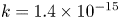 $k = 1.4 \times 10^{-15}$ m
 $^{2}$ and porosity
  $\phi =0.15$. The seals have thickness
  $h_f = 50$ m and are cut by a fault of width
  $d_f = 9$ m (measured from drill core) with porosity
  $\phi _f=0.07$ (Kampman et al. Reference Kampman2014). The system is initially saturated with water of density
  $\rho _a = 1000$ kg m
 $^{-3}$. Less dense CO
 $_2$ is injected at a constant rate of 0.1 Mt yr
 $^{-1}$ at the bottom of layer 1, and assumed to have constant density
  $\rho = 790$ kg m
 $^{-3}$ and dynamic viscosity
  $\mu = 6.9 \times 10^{-5}$ Pa s, calculated at typical storage reservoir conditions of 15 MPa and 40
  $^{\circ }$C (Dubacq, Bickle & Evans Reference Dubacq, Bickle and Evans2013). The mass flux of injected CO
 $_2$ is converted into a two-dimensional input flux assuming an along-fault system length of 1 km. These parameters give an initial value of
  $\lambda = 0.26$.

Figure 14. (a) Schematic showing injection of CO $_2$ into a system with multiple stacked aquifers and seals with a fault cutting through the layers. (b) The total CO
 $_2$ mass in each layer as well as the total leaked CO
 $_2$ (leakage from layer 3) plotted as a function of time for three different values of the fault permeability. The breakthrough time into each layer is marked with a grey vertical line.
The total CO $_2$ mass in each layer as well as the total leaked CO
 $_2$ (defined as the leakage from layer 3) is plotted as a function of time for three different values of the fault permeability (figure 14b). When the fault permeability is comparable to or less than the reservoir permeability, the majority of the CO
 $_2$ remains trapped within layer 1 after a 1000 year time scale. However, when the fault permeability is larger than the reservoir permeability, a significant fraction of the injected CO
 $_2$ leaks all the way through the system. For example, in the two cases where
  $k_f/k = 5$ and
  $k_f/k = 10$, layers 2 and 3 do not accumulate significant amounts of CO
 $_2$. However, even with
  $k_f/k = 10\,\%\sim 55\,\%$ of the CO
 $_2$ remains trapped after 1000 years. Note that this is the simple case where all layers have equal permeabilities. In a more realistic system where the permeability varies across layers, it is likely that larger accumulations of CO
 $_2$ would be seen in more permeable aquifers, regardless of their position. This system represents the worst case scenario for CO
 $_2$ storage as trapping mechanisms such as capillary trapping and dissolution trapping are neglected. In reality, as the CO
 $_2$ rises and spreads out into different aquifers these other mechanisms would contribute towards long-term storage of the CO
 $_2$.
$_2$.
7. Discussion
We have presented a new analytical model that describes the dynamics of leakage through a fault zone given properties relating to fault, aquifer and fluids. This new model has been tested against results from analogue porous medium tank experiments, from which we obtain good fits with the experimental data. This model has then been applied to predict the CO $_2$ distribution and leakage rates from a naturally occurring CO
 $_2$ reservoir. We find that when the permeability of the fault is comparable to the reservoir, the majority (>96 %) of the CO
 $_2$ remains trapped after 1000 years. However, it is important to highlight the limitations of the current model and discuss to what extent it can be applied directly in its present form, and in which ways it might be fruitfully enhanced as part of a future study.
The gravity current model uses a sharp-interface approximation (Huppert & Woods Reference Huppert and Woods1995; Hesse et al. Reference Hesse, Tchelepi, Cantwel and Orr2007), originally developed for miscible flows in porous media. This is valid for settings such as saline intrusions, but extra multiphase effects need to be considered when applied to immiscible settings such as CO $_2$–water systems (Golding et al. Reference Golding, Neufeld, Hesse and Huppert2011). When CO
 $_2$ is injected into water-saturated reservoirs, capillary forces play a key role in determining the saturation distribution and flow properties through the relative permeability and capillary pressure relationships (Nordbotten & Celia Reference Nordbotten and Celia2011). When the fault and reservoir have relatively uniform permeability, we expect the behaviour of the system to scale in a similar manner to the miscible case, with the effective permeability instead replaced by the product of intrinsic and relative permeability. However, geologically heterogeneous reservoirs may have significant gradients in capillary pressure, which tend to rearrange the CO
 $_2$ saturation into high permeability regions, thereby accelerating plume migration (Jackson et al. Reference Jackson, Agada, Reynolds and Krevor2018; Benham, Bickle & Neufeld Reference Benham, Bickle and Neufeld2021). An extension of the present model to fault zones with significant capillary heterogeneity therefore remains an outstanding and important question in predicting the flux through such systems.
Another potential refinement to the model is that the fault zone will have a capillary entry pressure that needs to be overcome before leakage can occur and so the underlying current may have to build up to a large thickness before breakthrough can occur. It is also possible that the CO $_2$ will be constrained to more localised flow paths with lower entry pressures which, depending on the entry pressure and permeability of the fault and intervening reservoirs, may affect the vertical migration of CO
 $_2$. These may be simply accommodated by the addition of a critical height the gravity current must overcome to achieve breakthrough in the fault (Woods & Farcas Reference Woods and Farcas2009; Sayag & Neufeld Reference Sayag and Neufeld2016).
The present gravity current model also assumes that the aquifer is unconfined ( $h \ll H$). This means that there is negligible flow of the ambient fluid and so fluid propagation is independent of the viscosity ratio between the fluids (Huppert & Woods Reference Huppert and Woods1995; Vella & Huppert Reference Vella and Huppert2006). Pegler, Huppert & Neufeld (Reference Pegler, Huppert and Neufeld2014a) showed that background pressure-driven flow due to confinement starts to play a role when ratio of the current depth and aquifer depth (
 $h/H$) is comparable to the viscosity ratio of the injected and ambient fluid. In the case of CO
 $_2$ and water, the viscosity ratio
  $\mu _{\textrm {CO}_2}/\mu _{w}\simeq 0.1$, hence the assumption that the size of the reservoir is much larger than the thickness of the current is valid for currents up to
  $\sim$10 % of the height of the aquifer, as is the case at many CO
 $_2$ storage sites. As the experiments performed in this study were between fluids of near equal viscosity, the thickness of the currents across all experiments are well within the limit for the unconfined approximation. For cases in which
 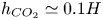 $h_{CO_2}\simeq 0.1H$, Pegler et al. (Reference Pegler, Huppert and Neufeld2014b) found that confinement causes greater leakage at earlier times due to the introduction of background pressure, but at later times, as the CO
 $_2$ fills the entire depth of the aquifer, the maximum hydrostatic head below the fracture is limited and hence the leakage rate is also limited. Incorporating the effects of confinement on the gravity current therefore also presents an additional extension of the present work.
There are other important fluid dynamical processes which stabilise the storage of CO $_2$, including for example the dissolution of CO
 $_2$ into the brine. Dissolution depends on the relative flows of CO
 $_2$ and brine over the small (e.g. centimetre) length scales related to CO
 $_2$ diffusion, presenting significant modelling challenges. However, the mixing of CO
 $_2$ and brine within the rising plumes and fault zone is likely to enhance dissolution of the CO
 $_2$ (cf. Kampman et al. Reference Kampman2014).
Constraining the hydraulic properties of fault zones in the field remains a much studied area with many different factors affecting the flow of fluids, such as the host rock composition (Wibberley & Shimamoto Reference Wibberley and Shimamoto2003), fracture density (Mitchell & Faulkner Reference Mitchell and Faulkner2012) and fracture connectivity (Sævik & Nixon Reference Sævik and Nixon2017) and their contributions to the overall permeability. The model presented in this study constrains the sensitivity of CO $_2$ leakage rates to bulk fault properties such as permeability, width and thickness. By observing the resultant plume behaviour around complex fault zones, this simplified model could be used to provide an estimate of these bulk properties. When applied in a suitable geological context, the model presented here can be used to characterise the flow dynamics of fault zones.
8. Summary and conclusions
We have presented an analytical model that describes the dynamics of leakage through a fault zone, motivated by the potential risk to storage security of anthropogenic CO $_2$. It comprises a two-dimensional gravity current in a porous medium, fed by a buoyant plume and spreading under a horizontal impermeable baffle. The medium is bounded by an impermeable vertical boundary and the horizontal baffle contains a fault through which the current is leaking. This system constitutes a reduced-order model of a faulted caprock, whereby an impermeable fault core is surrounded by a high permeability fracture zone (Wibberley et al. Reference Wibberley, Yielding and Toro2008) through which leakage occurs.
In the experiments, we observed thinning of the secondary plume above the fault due to an increase in Darcy velocity, leading to increased pressure gradients across the fault. A new model for leakage through the fault was derived, factoring in this effect. In contrast to previous analytical fault models which use numerical solvers to verify their models (Kang et al. Reference Kang, Nordbotten, Doster and Celia2014), we matched results using a series of analogous porous medium tank experiments, which supported the dependence of the fault width, fault height, input flux and input density on leakage rates as derived by the model. Crucially, this study showed how these parameters control the ratio of fluid flux into the aquifer compared with fluid leaking through the fault, which is significant for storage efficiency.
We demonstrated the utility of the model for assessment of storage security of anthropogenic CO $_2$ by application to a naturally occurring CO
 $_2$-charged aquifer at Green River, Utah, using an extension of the model to calculate the fluid distribution and leakage rates across multiple vertically stacked aquifers, cross-cut by a fault. This showed the dependence of leakage rates on the fault/aquifer permeability contrast, with significant leakage occurring when the fault permeability is larger than the reservoir permeability. A detailed discussion of the limitations of the model in application to CO
 $_2$–water systems was provided in § 7.
It is important to note that while other trapping mechanisms such as dissolution trapping, residual trapping and mineral trapping are important in CO $_2$ storage, they occur on longer time scales and so structural trapping remains the principal mechanism for storage of CO
 $_2$. Understanding to what extent faults within caprocks can act as potential leakage pathways is crucial for ensuring safe storage of CO
 $_2$.
$_2$.
Supplementary material
Supplementary material is available at https://doi.org/10.1017/jfm.2021.970.
Acknowledgements
The authors would like to acknowledge the many productive discussions had with A. Butler and the assistance from A. Pluck in building the experimental rig.
Funding
K.A.G. was funded by an Industrial CASE studentship from EPSRC and Shell (grant no. EP/P510440/1). This research is a contribution from the GeoCquest consortium, a BHP-supported collaborative project between Cambridge, Stanford and Melbourne Universities and supported by funding from a NERC Highlights grant (Grant No. NE/N016084/1).
Declaration of interests
The authors report no conflict of interest.
Appendix A. Late time behaviour of current horizontal extent
Assuming that changes to the shape of the current are small at late times, the time derivative of (2.29) is
 \begin{equation} \phi \kappa \frac{{\textrm{d}}}{{\textrm{d}}t}[h_0 x_N] \approx q - q_F, \end{equation}
where  $\kappa$ represents the dimensionless volume of the current (e.g.
  $\kappa = 1/2$ in the case of a triangle) and the leakage flux
 \begin{equation} q_F = \frac{\zeta q}{h_f}(h_0 + h_f), \end{equation}
with  $\zeta = {d_f \phi _f k_f g'}/{\nu q}$. From (2.28a), we obtain the relationship
 \begin{equation} \left. -\frac{kg'}{\nu} h_0 \frac{\partial h}{\partial x}\right|_{x=0} = q - q_F. \end{equation}
At late times, we can approximate
 \begin{equation} \left. \frac{\partial h}{\partial x}\right|_{x=0} \approx{-}\frac{h_0}{x_N}. \end{equation}
At the equilibrium point where  $q_F \to q$, the thickness of the current at
  $x=0$
$x=0$
 \begin{equation} h_0 \to h_f\left(\frac{1}{\zeta} - 1\right) = h_{0\infty}, \end{equation}
which is obtained from (A2). We consider the current thickness at  $x=0$,
 \begin{equation} h_0 = h_{0\infty} - \delta(t), \end{equation}
where  $\delta (t)\ll h_{0\infty }$ is a small perturbation. On equating (A1) and (A3) and applying the relationships (A4) and (A6),
 \begin{equation} \phi \kappa \frac{{\textrm{d}}}{{\textrm{d}}t}[(h_{0\infty}-\delta(t)) x_N] \approx \frac{kg'}{\nu x_N}(h_{0\infty}-\delta(t))^{2}. \end{equation}
By considering the leading-order terms, we find that
 \begin{equation} x_N \approx \left(\frac{k g' h_{0\infty}}{\phi \kappa \nu } t\right)^{1/2}, \end{equation}
which indicates that the current extent follows a  $t^{1/2}$ power law relationship at late times.
Appendix B. Functional form of calibration curve
A series of calibration experiments were performed to determine the functional relationship between the image intensity and dye concentration. In each calibration experiment, the cell was uniformly saturated with a red dye solution with concentration  $C_d$. A total of 20 different concentrations between 0 and
  $3.00 \pm 0.05$ g l
 $^{-1}$ were used to construct the calibration curve. The light intensity for each dye concentration was calculated by subtracting the average green or blue colour channel across the image from the average green or blue channel across a reference image where
  $C_d = 0$ g l
 $^{-1}$. The green and blue channel produce unique calibration curves (figure 9) which are sensitive to changes in image intensity at different concentrations.
The functional forms of the calibration curves for the green and blue channels are
 \begin{equation} C_G = aI_G^{4} + bI_G^{3} + cI_G^{2} + dI_G, \end{equation}
and
 \begin{equation} C_B = \begin{cases} aI_B, & I \leq 106,\\ (b + cI_B)^{{-}1/d},& I > 106, \end{cases} \end{equation}
where  $I_G$ and
  $I_B$ are differences in the green or blue image intensity between the reference and calibration images and
  $a$,
$a$,  $b$,
$b$,  $c$ and
  $d$ are fitting coefficients.
The calibration curve for the blue channel is sensitive to small changes in dye concentration for concentrations up to  $\sim$0.9 g l
 $^{-1}$, but insensitive at higher concentrations due to image saturation. In comparison, the green channel is less sensitive at low concentrations but has greater sensitivity at dye concentrations above 0.9 g l
 $^{-1}$. The best calibration results are obtained when using a weighted average of the two curves to convert image intensity to dye concentration. The effective concentration is determined by the function
 \begin{equation} C_{eff} = C_B + \left(\frac{C_G - C_B}{2}\right)\left[1+\tanh{\left(\frac{C_{avg}-\tau}{\delta}\right)}\right], \end{equation}
where  $C_B$ and
  $C_G$ are the concentrations calculated from the blue and green calibration curves,
  $C_{avg} = {(C_B + C_G)}/{2}$,
  $\tau$ is the concentration at which
  $C_{eff}$ is a result of equal contributions from
  $C_B$ and
  $C_G$ (grey solid line, figure 9) and
  $\delta$ sets the width of the region both curves contribute significantly towards
  $C_{eff}$ (grey dashed lines, figure 9). The calibration curves in figure 9 were calculated using an average light intensity across the full calibration images. Calibration curves were plotted for subregions of the cell to check for the potential effect of small variations in light intensity. However, it was found that effects of spatial variation were minimal.


 Open access