


1. Introduction
Supersonic flows exiting from a convergent–divergent nozzle are widely used in various scientific and industrial applications. The performance and efficiency of the nozzle in various operating conditions play a crucial role in numerous systems where supersonic open jets are present. Some of the significant examples are the thrust generation in jet engines, efficient mixing of the supersonic jets, mixing of fuel and jet in the scramjet combustion chamber, and ejector operation in refrigeration and high-altitude testing facilities. The off-design operation of the nozzle flows differs considerably from that of the design conditions and exhibits a wide variety of flow features involving complex interactions of shockwaves and expansion fans in the jet owing to the requirement of the pressure matching conditions. Tam (Reference Tam1987) studied the noise generation from overexpanded jets and concluded that the interaction of shockwaves and the expansion fans with the ambient flow through the shear layer is the primary source of the jet noise. Thus, the study and understanding of the imperfectly expanded supersonic flow from the nozzle are necessary to improve and optimise the nozzle's performance and efficiency during off-design operations. The changes in the flow characteristics in the imperfectly expanded jets can help us understand the jet noise generation. A better understanding of the shock reflection/interaction phenomenon in the open jet helps in the design and development of quieter jet engines for various aircraft.
Courant & Friedrichs (Reference Courant and Friedrichs1999) were the first to discuss the transition of the shock wave reflections from the Mach reflection (MR) to the regular reflection (RR) in an imperfectly expanded jet. The early studies of shock transitions were mainly focused on those that appear in the axisymmetric open jets because of their broad applicability in industrial and defence applications. The investigation of overexpanded planar nozzle flows received less attention, and the mechanism of shock interaction and the transition is not understood fully in the case of imperfectly expanded open jets. Some of the important works on the shock interactions in the supersonic planar jets were carried out by Hadjadj, Kudryavtsev & Ivanov (Reference Hadjadj, Kudryavtsev and Ivanov2004), Shimshi, Ben-Dor & Levy (Reference Shimshi, Ben-Dor and Levy2009) and Chow & Chang (Reference Chow and Chang1975). Hadjadj et al. (Reference Hadjadj, Kudryavtsev and Ivanov2004) numerically studied the shock interactions in the overexpanded planar jets using the inviscid and viscous simulations and examined the hysteresis in the shock transitions. Shimshi et al. (Reference Shimshi, Ben-Dor and Levy2009) studied the shock interactions and investigated the hysteresis in highly overexpanded jets. Chow & Chang (Reference Chow and Chang1975) used the method of characteristics and studied the imperfectly expanded jets, and estimated the Mach stem size in the planar flow field. Tam (Reference Tam1987) and Tam & Chen (Reference Tam and Chen1994) studied the turbulent mixing noise from the overexpanded supersonic jets and concluded that the shock associated noise is much higher compared with the turbulent mixing noise in the jet. Menon & Skews (Reference Menon and Skews2010) analysed the evolution of rectangular jets and other non-axisymmetric jets for various pressure ratios corresponding to the underexpanded regime and observed that the shock transition process depends on the aspect ratio and shape of the nozzle exit. Experimental and computational studies of the shock interactions in the overexpanded axisymmetric jets have been carried out by Matsuo et al. (Reference Matsuo, Setoguchi, Nagao, Alam and Kim2011). They experimentally verified the presence of shock transition in the overexpanded jets for different nozzles exit Mach numbers. A detailed review of the experimental and computational works carried out in the underexpanded axisymmetric jets is presented by Franquet et al. (Reference Franquet, Perrier, Gibout and Bruel2015). Gribben, Badcock & Richards (Reference Gribben, Badcock and Richards2000) numerically studied the shock hysteresis phenomenon in the underexpanded jets in two-dimensional (2-D) planar flows and confirmed the presence of hysteresis in the shock transition.
From the above literature, it is understood that adequate knowledge of the imperfectly expanded nozzle flows exists. Most of the studies reasonably explain the jet structures and associated flow processes. It is known from the above studies that the characteristic changes in imperfectly expanded jet owing to the change in pressure ratios are mainly attributed to the changing shock interaction patterns in the flow field, while the upstream Mach number (exit Mach number in the case of the nozzle) is held constant in an inviscid scenario. The shock transitions such as wedge angle variation induced transition and upstream Mach number variation induced transition are relatively well understood, and the transitions lines are identified in steady supersonic flows over wedges (Ben-Dor Reference Ben-Dor2007). However, the case of open jets will be considerably different from its wedge counterpart wherein the former, the free stream Mach number (nozzle exit Mach number) is fixed, and the shock interactions change their characteristics owing to the variation in the pressure ratios in the jet. It would hence be interesting to see whether the shock reflection patterns in the open jet are analogous to that of the wedge flows, where the transitions are due to wedge angle variation or upstream Mach number variation, and the steady transition criteria such as von Neumann, sonic and detachment criteria in wedge flows are applicable in the case of jet flows as well. The most important flow feature of an MR is the Mach stem, a finite length scale in the flow field, and a near-normal shock that causes profound changes in the flow field due to its high-pressure and temperature conditions downstream of it. There have been estimates on the Mach stem size of an MR in wedge flows where the overall configuration of the MR was analytically modelled previously (Li & Ben-Dor Reference Li and Ben-Dor1997a; Mouton & Hornung Reference Mouton and Hornung2007; Bai & Wu Reference Bai and Wu2017). It is also known that the MR–RR transition at the von Neumann condition (Ben-Dor Reference Ben-Dor2007) can be identified by the process of Mach stem height going to zero. In a previous work of Li & Ben-Dor (Reference Li and Ben-Dor1997b), it has been shown that the mechanism responsible for the existence of the steady MR configuration in open jets is essentially the same as that in the case of reflection of a wedge-generated shock wave. They also developed an analytical model to estimate the Mach stem height in the open jets based on the model developed in their previous work (Li & Ben-Dor Reference Li and Ben-Dor1997a), for the wedge flows. However, as the Mach stem is a finite length scale in the flow field, its size would be decided by the flow configurations and the geometric parameters such as the inlet height, the wedge length, wedge angle and the trailing edge height of the wedge (Hornung & Robinson Reference Hornung and Robinson1982). Based on this aspect, the claim of a similar Mach reflection configuration in the overexpanded open jets as that in the case of wedge flow becomes questionable, as there may not be an analogy for the wedge length, wedge angle and trailing height when compared with the case of the open jet shock configurations.
Moreover, in the open jet, a predominant phenomenon is absent from the wedge flows, which is the expansion fan–reflected shock interaction. The absence of the interaction may lead to subsequent changes in the reflection configuration such as the rate at which a Mach stem grows/shrinks within the dual domain (Ben-Dor Reference Ben-Dor2007) or beyond the detachment criterion, the nature of the hysteresis, and how the transition occurs at von Neumann condition in the steady/quasi-steady scenario. In addition to the above inviscid aspects, the viscous effects may play vital roles in determining the shock reflection structures. While in the wedge flows, the boundary layer developed on the wedge alters the transition shock angles, there is no such mechanism in jet flows where the shock/expansion fan develops over the jet boundary/shear layer.
Hence, it is essential to understand the significant differences between the shock reflections in the overexpanded open jets and the wedge flows based on the above aspects, as the well known facts on the wedge angle variation induced  $RR \rightleftharpoons MR$ transition cannot be simply extended to the open jet shock interactions and assess the off-design performance of the supersonic nozzle. The present study attempts to bring out the characteristic features of the shock reflections in open jets emphasising the estimation of overall Mach reflection configuration, how the transition points are arrived at, and the nature of hysteresis through analytical and higher-order numerical simulations. Experiments have also been conducted to estimate the Mach stem size for various pressure ratios. The study is expected to give a clear idea of the differences between the shock reflections on wedge flows and the open jets, which were believed to have similar flow features and analysed using the same assumptions in the previous research works. It also elucidates how the open jet MR configuration represents a crucial limiting case of the wedge flows. The estimation of the Mach stem height in the open jet is carried out by extending the method developed for the wedge flows by Li & Ben-Dor (Reference Li and Ben-Dor1997a), Mouton & Hornung (Reference Mouton and Hornung2007) and Bai & Wu (Reference Bai and Wu2017). These methods are the prominent models used in the estimation of Mach stem height in the wedge flows. The above models are appropriately modified to calculate the Mach stem height in the open jets, and these modifications are discussed in the subsequent sections.
The present paper is structured in the following way. We start with the operation of the nozzle and its various regimes in the flow field in § 2. The analytical formulation of the Mach stem height in the open jets is derived in §§ 3 and 4. The computational methodology is discussed in § 5, and the experimental methodology in § 6. Section 7.1 starts with the comparison of the Li & Ben-Dor (Reference Li and Ben-Dor1997b) method and the modified Li and Ben-Dor method presented in this work. Sections 7.2 and 7.3 compare the results from the analytical model with the computational and experimental results. Section 7.4 discusses the essential difference that occurs in the open jet MR configuration compared with the wedge flows and highlight the crucial attribute of the open jet MR configuration. Section 7.5 discusses the MR's growth rate in the open jets, and the wedge flows. Sections 7.6 and 7.7 discuss the MR configuration as the nozzle operation is changed and the hysteresis phenomenon, respectively. Section 8 concludes the present work and discusses the possibilities and extension of the current work.
2. Inviscid operating regimes in overexpanded nozzles
Inviscid supersonic flow from a planar convergent–divergent nozzle can be classified as overexpanded or underexpanded jets based on the nozzle pressure ratio (NPR), i.e. the ratio of the stagnation chamber pressure to the ambient pressure  $(P_o/P_b)$. In both the regimes, shock wave interactions exist over a wide range of NPR values, and the schematic of various shock reflection configurations that occur in an overexpanded jet is shown in figure 1. Various regimes of shock reflections present in the inviscid open jets of different exit Mach numbers are shown in figure 2 (Arun Kumar & Rajesh Reference Arun Kumar and Rajesh2017). The appearance of the supersonic flow at the exit of the nozzle starts when the NPR becomes more than the second critical pressure ratio (the pressure ratio at which the normal shock wave stands at the exit plane of the nozzle) which is shown in the figure 1(a). Beyond the second critical pressure ratio, as the NPR increases, the flow exits the nozzle at the design supersonic Mach number with a pressure lower than the surrounding ambient pressure. This regime is denoted as the overexpanded regime. The main characteristic of this regime is the presence of shockwaves at the exit of the nozzle to match the flow pressure with the ambient pressure.

Figure 1. Shock reflection in inviscid overexpanded jets. (a) second critical pressure; (b) subsonic flow behind the incident shock; (c) sonic flow behind the incident shock; (d) MR; (e) RR.
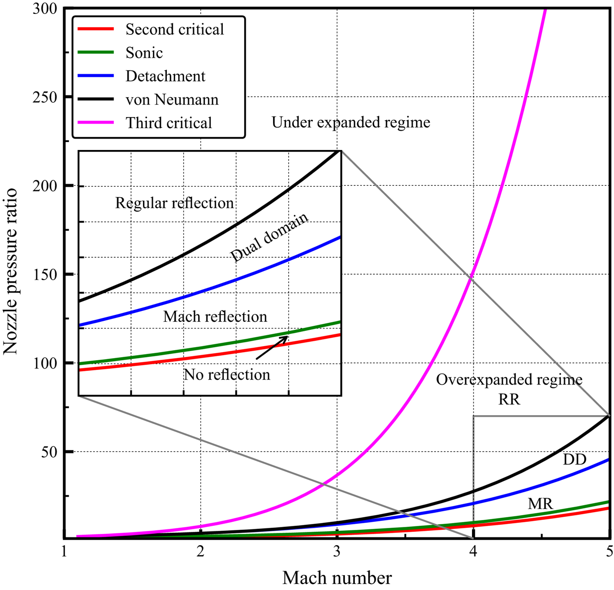
Figure 2. Different regimes of flow field present in the imperfectly expanded jet for various Mach numbers. The dual-domain regime is shown as DD (Arun Kumar & Rajesh Reference Arun Kumar and Rajesh2017).
Beyond the second critical pressure ratio, the incident shock in this regime is initially strong enough that there will be subsonic flow behind the shockwave, and the reflection is not possible because of the strong oblique shock waves in the flow field as shown in figure 1(b). The reflection in the jet starts when the flow behind the incident shock wave achieves the sonic condition as shown in figure 1(c), and a Mach reflection develops in the flow based on the NPR as shown in figure 1(d). The reason for the appearance of the Mach reflection is that at low NPR, incident shock is strong, and its strength decreases as the NPR is increased. The strong incident shock creates a small flow Mach number behind it and a large turning angle. The requirement of a large flow turning angle by the reflected shock wave would lead to an impossible scenario to form a RR and result in the appearance of the MR configuration at lower NPR in the overexpanded jets, as shown in figure 1.
The schematic of the MR and RR configuration is shown in figure 1 and the corresponding shock polar solution for each reflection is shown in figure 3. The essential flow features of the MR and RR configurations such as shock waves, expansion fans and sliplines, are seen in figure 1. The effect of increase in NPR will result in decreasing pressure jump across the incident (lip) shockwave. The decrease in the pressure jump reduces the strength of the incident shock wave, leading to increased downstream Mach number and decreased flow turning angle. As the turning angle decreases, the shock structure will undergo a transition from the MR to the RR configuration. This transition of the shock structure occurs at the detachment condition (Ben-Dor Reference Ben-Dor2007). For any NPR below this point, only MR exits, and the RR is not possible. The detachment condition is a function of NPR and the nozzle exit Mach number, as shown in figure 2 for various Mach numbers. Figure 2 also shows another critical transition condition present in the supersonic flow field, i.e. the von Neumann condition (Ben-Dor Reference Ben-Dor2007). For NPR above the von Neumann condition, only an RR solution is possible. The analytical method developed in the present work can be applied to the overexpanded regime where the flow behind the reflected shock is supersonic in nature. The current analytical model does not consider the direction of operation of the nozzle, i.e. whether the NPR is increased or decreased to attain the given NPR. Thus the model can predict the Mach stem height for a given NPR and Mach number of the jet without considering the operation of the nozzle. As can be seen later from §§ 7.2 and 7.3, the MR configuration in the open jets depends mainly on three different parameters as given in (2.1), i.e. specific heat ratio ( $\gamma$), Mach number of the jet (M) and NPR,
 \begin{equation} \frac{H_m}{H} = f(\gamma, M, NPR). \end{equation}
Figure 3. Shock polar solution showing MR and RR configuration in overexpanded jets.
3. MR configuration in open jets and wedge flows
The Mach reflection structure and the flow field of the overexpanded jets differ appreciably from those on the supersonic wedge flow configuration. The shock reflection in the free jets occurs due to the pressure imbalance between the jet and the surrounding ambient gas, while the shock reflection in the wedge flow is primarily to achieve the flow tangency condition as the flow conforms to the wedge surface. The significant difference in the shock structure comes from the interaction of the shock wave and the expansion fan with the free shear layer, i.e. jet boundary present in the flow field. A similar interaction is absent in the wedge flows, where the MR becomes impossible if the shock wave interacts with the wedge surface, which is a solid wall (Landau & Lifshitz Reference Landau and Lifshitz1987). The shock structure in the overexpanded jets is susceptible to the instabilities in the jet boundary (Kelvin–Helmholtz instability) that will further grow due to the interaction with the reflected shock wave. The other key difference is the absence of the interaction of the expansion fan with the reflected shock wave (Li & Ben-Dor Reference Li and Ben-Dor1997a), which may significantly alter the MR shock structure in the overexpanded jets compared with the wedge flows. The interaction of the reflected shock wave with the expansion fan weakens the latter, thereby affecting the location of the sonic throat formation in the subsonic duct generated by the Mach stem. This change in the sonic throat location may considerably vary the Mach stem size and location. In the wedge flows, the expansion fan communicates the wedge length to the Mach stem via its interaction with the reflected shock wave and the slipline, which decides the Mach stem size in the flow field. Another critical difference between the wedge flows and the overexpanded jet is the existence of stable MR configurations in the overexpanded jets for all possible NPR above the detachment criterion. In contrast to the possibility of stable Mach reflection in the overexpanded jets, the wedge flows do not guarantee a stable MR configuration for all the wedge angles and wedge length combinations. This is due to the dependence of the MR configuration on the physical lengths in the flow field, such as the wedge length and the inlet opening, which govern the existence of the stable MR configuration and the Mach stem size – a length scale in the flow field. Thus, the size of the Mach stem has bounds, and the MR may exist only for a specific range of combinations of the physical lengths and wedge angles for a given Mach number (Li & Ben-Dor Reference Li and Ben-Dor1997a) and can have multiple MR configurations depending on the physical lengths described above. However, the MR structure in the open jet is unique for the given NPR and the nozzle exit Mach number. The absence of the physical length scales in the overexpanded jet sets it apart from its counterpart, i.e. wedge flows. Another significant feature of the overexpanded jet is the continuously changing jet boundary length as the NPR is changed in contrast to the wedge flows where the wedge length is fixed for a given Mach number. Thus, the rate of change of Mach stem growth and the MR structure will seemingly differ in both systems, making the comparison of the flow phenomena difficult. To accurately compare the MR structure in the wedge and open jets, wedge length needs to be fixed equal to that of the jet boundary length in the overexpanded jet for every wedge angle. Once the wedge length for a given wedge angle is fixed, the resulting MR reflection structure that occurs as the reflected shock wave hits the wedge corner, the condition which is referred to as  $H_{t,min}$ (MR) (Li & Ben-Dor Reference Li and Ben-Dor1997a), will be identical to the overexpanded jets according to the quasi-one-dimensional approximation. The analytical method should predict the same values for the Mach stem height for both cases, which can be used to ascertain the validity of the analytical approach to open jets. Despite the differences discussed above in the Mach reflection structure between the wedge flows and the open jet, the models developed for the wedge flow to estimate the Mach stem height provide an excellent basis for modelling the Mach reflection configuration in the open jets. Li & Ben-Dor (Reference Li and Ben-Dor1997b) extended the Mach stem height estimation of wedge flows (Li & Ben-Dor Reference Li and Ben-Dor1997a) to the 2-D overexpanded jets. Their primary assumptions involve that the Mach stem height can be modelled similarly to that of the wedge flow without any significant modifications to the physics of the flow field in overexpanded jets. The model removes the shock wave and expansion fan interaction from the wedge model and makes an additional assumption of first-order approximation to the curvature of the slipline as the expansion fan interacts with it. The reduction in the complexity of this analytical model compared with the wedge model resulted in a closed-form expression for the Mach stem height for the given NPR and Mach number of the open jet. In the present study, the Mouton & Hornung (Reference Mouton and Hornung2007) and the Bai & Wu (Reference Bai and Wu2017) methods developed for wedge flows will be extended to overexpanded jets and the Li & Ben-Dor (Reference Li and Ben-Dor1997b) method will be improved by modifying the first-order approximation to the curvature of the slipline. The Li and Ben-Dor method is chosen for including all the relevant flow physics in the estimation of Mach stem and is also simpler to solve when compared with other recent methods developed by Gao & Wu (Reference Gao and Wu2010). The Mouton & Hornung (Reference Mouton and Hornung2007) method is chosen for its more straightforward geometric approach to estimate the Mach stem height. The Bai & Wu (Reference Bai and Wu2017) method is included as it models the subtle but vital wave interactions happening on the slipline and is a modified model of that proposed by Gao & Wu (Reference Gao and Wu2010). The detailed description of the extension of analytical models to the overexpanded jet is explained in the following sections.
4. Analytical formulation of Mach stem height
4.1. Li and Ben-Dor method for overexpanded jets
The method developed in Li & Ben-Dor (Reference Li and Ben-Dor1997a) and Li & Ben-Dor (Reference Li and Ben-Dor1997b) for estimating the Mach stem height in the wedge flows and the overexpanded jets are described briefly. The geometric parameters of the overexpanded jet are derived again and solved similarly to that of the wedge flow. The primary assumptions are that the flow is steady, ideal and obeys the perfect gas equation of state. The slipline is assumed to be infinitely thin, and the Mach stem and the slipstreams form a converging duct where the subsonic flow is accelerated isentropically. At some point in the slipline, the sonic throat forms after the interaction with the expansion fan. The MR configuration as depicted by Li & Ben-Dor (Reference Li and Ben-Dor1997b), consisting of the incident shock ( $i$), reflected shock (
 $r$), Mach stem (
 $m$), slipline (
 $s$), jet boundary (
 $J$), triple point (
 $T$), nozzle exit height (
 $H$), Mach stem height (
 $H_m$) and sonic throat height (
 $H_s$) is shown in figure 4.

Figure 4. Schematic of overexpanded jet Mach reflection configuration for Li and Ben-Dor Method. The flow angles and the shock angles are marked along with the critical points used in the geometric construction. Abbreviations are: incident wave ( $i$); reflected wave (
 $r$); Mach stem (
 $m$); triple point (
 $T$); jet boundary (
 $J$).
$J$).
The estimation of Mach stem height starts with obtaining a solution close to the triple point. To solve the flow field near the triple point ( $T$), the conservation equations/oblique shock relations are solved with the appropriate boundary conditions (i.e. the solution to the three-shock theory of von Neumann). These relations are given in Appendix A. Once the three-shock theory is solved, flow properties close to the triple point are known. The next step in the algorithm is to solve the expansion fan interaction with the slipline. The amount of flow deflection needed for the expansion fan to make the flow parallel behind the reflected shock is calculated using the isentropic relations and Prandtl–Meyer relations for the expansion fan as given in Appendix A. Solving the flow behind the reflected shock wave will provide the necessary information about the geometric quantities needed to calculate the characteristics of the expansion fan that creates the sonic point. The subsonic flow in the convergent duct behind the Mach stem is subsequently solved.
The following equation gives the area–Mach number relationship in the subsonic pocket:
 \begin{equation} \frac{H_m}{H_s}=\frac{1}{\bar{M}}\left[\frac{2}{\gamma+1}+\frac{(\gamma-1)}{(\gamma+1)} \bar{M}^2\right]^{({\gamma+1})/{2(\gamma-1)}} . \end{equation}
where  $H_m$ denotes the Mach stem height,
  $H_s$ denotes the sonic throat and
  $\bar {M}$ denotes the mass averaged Mach number behind the Mach stem. Thus, all the flow parameters required to calculate the Mach stem are evaluated, and the final step is the generation of a closed set of geometrical relations needed to calculate the Mach stem height. The geometrical relationships are obtained similarly to Li & Ben-Dor (Reference Li and Ben-Dor1997a) model from figure 4 and are as follows:
 $$\begin{gather} X_T\tan\beta_1=H-H_m, \end{gather}$$
 $$\begin{gather}X_D\tan\theta_1=H-Y_D, \end{gather}$$
 $$\begin{gather}(X_D-X_T)\tan(\beta_2-\theta_1)=Y_D-H_m, \end{gather}$$
 $$\begin{gather}(X_F-X_T)\tan\theta_3=H_m-Y_F, \end{gather}$$
 $$\begin{gather}(X_E-X_D)\tan\mu_D=Y_D-H_s, \end{gather}$$
 $$\begin{gather}(X_F-X_D)\tan(\mu_2+\theta_3)=Y_F-Y_D, \end{gather}$$
 $$\begin{gather}(X_E-X_F)\tan\theta_3=(2+\tan^2\theta_3)(Y_F-H_s). \end{gather}$$
 There are seven geometric relations and eight unknowns. The above set of equations can be closed along with (4.1), i.e. the area–Mach number relation obtained from the subsonic pocket analysis. The closed set of equations is solved using a nonlinear iterative solver in Python to obtain the Mach stem height and other flow field parameters. The significant modification of the present model compared with the Li & Ben-Dor (Reference Li and Ben-Dor1997b) model for the overexpanded jets is the modelling approximation for the curved slipline shown in figure 4. The curved slipline labelled ‘FE’ is modelled in the Li & Ben-Dor (Reference Li and Ben-Dor1997b) using (4.3) instead of the one given as (4.2g) in the present derivation. The following equation is a special case of (4.2g) where the approximation  $| \theta _3 | \ll 1 \implies tan^2 \theta _3 \approx 0$ holds:
 \begin{equation} \tan\theta_3=2\frac{Y_F-H_s}{X_E-X_F}. \end{equation}
 The value of the slipline angle  $\theta _3$ varies as the NPR changes continuously. The above assumption may not be valid for all scenarios and all Mach numbers, and hence it is decided to retain the original equation derived from the Li & Ben-Dor (Reference Li and Ben-Dor1997a) model rather than to proceed with the approximation used in the Li & Ben-Dor (Reference Li and Ben-Dor1997b) model. The comparison between the present analytical model and the Li & Ben-Dor (Reference Li and Ben-Dor1997b) model will be discussed in the results (see § 7.1).
4.2. Mouton and Hornung method for overexpanded jets
Mouton & Hornung (Reference Mouton and Hornung2007) developed a geometrical method based on Azevedo & Liu (Reference Azevedo and Liu1993) to estimate Mach stem height in wedge flows. The method departs from Azevedo & Liu (Reference Azevedo and Liu1993) by assuming that the sonic throat occurs downstream of the leading expansion wave, where it interacts with the slipline from the triple point. The Mouton & Hornung (Reference Mouton and Hornung2007) method proves to be more accurate for specific Mach numbers and certain wedge angles than the Li & Ben-Dor (Reference Li and Ben-Dor1997a) method in the supersonic wedge flow. The Mouton & Hornung (Reference Mouton and Hornung2007) method also incorporates the growth rate of a Mach stem when the RR gets transitioned to MR in the dual-domain regime due to the disturbances in the flow field. In this method, the shocks and the slipline in the flow field are considered to be straight. The slipline is considered as a solid wall, and there exists a pressure discontinuity across the slipline. These are the primary assumptions that differ from the Li and Ben-Dor method to estimate Mach stem height. The method uses a self-consistent geometric constraint for the estimation of the Mach stem height.
In the present work, the method developed by Mouton & Hornung (Reference Mouton and Hornung2007) is extended to the planar nozzle flows to estimate the Mach stem height in the overexpanded jets. The schematic of the overexpanded flow field is shown in figure 4. The geometric equations that are modified for a 2-D planar nozzle are as follows:
 $$\begin{gather} AT\sin\beta_1+H_m=H, \end{gather}$$
 $$\begin{gather}TD\sin\phi+H_m=DF\sin\mu_D+H_s, \end{gather}$$
 $$\begin{gather}AD\cos\theta_1+DF\cos\mu_D=AT\cos\beta_1+(H_m-H_s)\cot\theta_3, \end{gather}$$
 $$\begin{gather}AT\sin\beta_1=AD\sin\theta_1+TD\sin\phi, \end{gather}$$
 $$\begin{gather}AT\cos\beta_1+TD\cos\phi=AD\cos\theta_1, \end{gather}$$
where  $H_m$ and
  $H_s$ denote the Mach stem height and the sonic throat height, respectively. Here
  $\theta _1$ represents the flow deflection angle,
  $\phi$ represents the angle between the horizontal and the reflected shock wave,
  $\beta _1$ represents the incident shock angle,
  $\mu _D$ represents the characteristic wave angle at the sonic throat location and
  $\theta _3$ represents the slipline angle. The solution at the triple point obtained from the three-shock theory, described in Appendix A, gives the necessary information about the shock angles, flow angles and the slipline angle at the triple point. This information can be used to calculate the value of
  $\phi = \beta _2 - \theta _1$. The amount of the characteristic wave angle at the sonic throat
  $\mu _D$ can be obtained using the Prandtl–Meyer relationship given in Appendix A and the fact that flow must turn an angle
  $\theta _3$ after the reflected shock before passing through the expansion fan at the sonic point. Once the equations for the three-shock theory and the expansion fan interaction are solved, the geometric relations needed for calculating the Mach stem height can be obtained from the schematic shown in figure 4. The geometric relationships are given in (4.4a)–(4.4e). The formulation has six unknowns and five equations. The area–Mach number relationship given in (4.1) relating the
  $H_m$ and
  $H_s$ closes the above set of equations. These are solved using a nonlinear iterative solver to obtain the Mach stem height for a given Mach number and NPR.
4.3. Bai and Wu method for overexpanded jets
Bai & Wu (Reference Bai and Wu2017) developed a comprehensive analytical method by considering the wave interactions that occur on the slipline due to the changes in the subsonic duct and the interaction of the expansion fan. This improved model is an extension of the work of Gao & Wu (Reference Gao and Wu2010) which gives an analytical relationship for the curvature and the slope of the slipline. The extension of the Bai & Wu (Reference Bai and Wu2017) method to model MR structure in the overexpanded jet is straightforward, and the algorithm is explained below. The schematic used in the Bai and Wu method is similar to that of the Li and Ben-Dor model, as shown in figure 4. At first, the flow parameters close to the triple point  $T$ are obtained using the three-shock theory. The slipline emanating from the triple point can be modelled as two different sections based on its interaction with the expansion fan. The slipline from the triple point to the first interaction point of the expansion fan, i.e. the curve labelled ‘TE’ in figure 4, is taken to be the free part of the slipline. The analytical relationships described in the Bai & Wu (Reference Bai and Wu2017) method can be applied without any modifications to this section of the slipline in the overexpanded jets. The curvature and the height of the slipline (labelled ‘TE’) can be calculated by solving the equations (4.5a)–(4.5e) simultaneously for given
  $\Delta x$. The following equations relate the pressure decrements above and below the slipline to the other flow parameters such as the Mach number and height of the slipline from the symmetry:
 $$\begin{gather} \frac{H_s}{H_m} = \frac{M_m N^{-\left(({\gamma+1})/{2\gamma}\right)}}{\sqrt{\dfrac{2}{\gamma-1}\left(\chi(M_m)N^{-\left(({\gamma-1})/{\gamma} \right)}\chi(M_s^+)-1\right)}}\left(\chi\left(M_s^+\right)\right)^{({\gamma+1})/{2(\gamma-1)}}, \end{gather}$$
 $$\begin{gather}\chi\left(M\right)=1+\frac{\gamma-1}{2}M^2, \end{gather}$$
 $$\begin{gather}N = \frac{p_2^T}{p_m}\left(\chi(M_2^T)\right)^{{\gamma}/({\gamma-1})}, \end{gather}$$
 $$\begin{gather}\nu(M_s^+)-\nu(M_2^T)=\theta_s -\theta_3, \end{gather}$$
 $$\begin{gather}\tan{\theta_s}={-}\frac{{\rm d}H_s}{{\rm d} x}={-}\frac{\Delta H_s}{\Delta x}, \end{gather}$$
where  $M_m$ and
  $M_s^+$ represent the flow Mach number behind the Mach stem and in the supersonic stream above the slipline, respectively,
  $M_2^T$ and
  $p_2^T$ represent the Mach number and pressure behind the reflected shockwave at the triple point
  $T$. Here
  $\theta _s$ and
  $\theta _3$ represent the slipline angle at the particular section and the slipline angle at the triple point. The parameters
  $\chi$ and
  $N$ in (4.5a) are defined in (4.5b) and (4.5c), respectively. The Prandtl–Meyer function
  $\nu$ given in (4.5d) is defined in Appendix A in (A10). Here
  $H_s$ and
  $H_m$ represent the subsonic duct height and the Mach stem height, respectively. These systems of (4.5a)–(4.5e) can be solved using any nonlinear solvers to calculate the flow properties along the free part of the slipline. The interaction part of the slipline (labelled ‘EF’) in the overexpanded jets needs modifications to exclude the interaction of the expansion fan with the reflected shockwave. The shape of the reflected shockwave is straight in the overexpanded jets as there is no interaction with the expansion fan and does not play a crucial role in the formation of the Mach stem as in the wedge flows. Likewise, the expressions for the expansion fan does not require any modelling as the regularised transmitted Mach wave since the expansion fan does not interact with the reflected shockwave. Hence the contributions of these effects are excluded from the modelling of the interaction part of the slipline (labelled ‘EF’). The modified equations are described through (4.6a)–(4.6d) as follows:
 $$\begin{gather} \frac{{\rm d} x}{{\rm d}\theta_t} ={-}\varGamma = \frac{{\tan}^2\left(\mu_t+\theta_t\right)+1}{\tan{\left(\mu_t+\theta_t\right)}-\tan{\delta_s}} \frac{M_t^2\ -1+\chi\left(M_t\right)}{M_t^2 -1}(x_s -X_D), \end{gather}$$
 $$\begin{gather}\frac{\gamma p_t M_t^2}{\sqrt{M_t^2 -1}}\left(\frac{{\rm d}\theta_s}{{\rm d}x_s}+\frac{1}{{\varGamma}} \right)+\frac{\gamma M_s^2}{1-M_s^2}\frac{p_s}{H_s}\tan{\delta_s}=0, \end{gather}$$
 $$\begin{gather}\frac{H_s}{H_t}=\frac{M_m}{M_s} \left(\frac{\chi\left(M_s\right)}{\chi\left(M_m\right)}\right)^{({\gamma+1})/{2(\gamma-1)}} , \end{gather}$$
 $$\begin{gather}\tan{\left(\theta_s\right)}={-}\frac{{\rm d}H_s}{{\rm d} x}={-}\frac{{\Delta}H_s}{{\Delta x}}. \end{gather}$$
 Equation (4.6b) models the flow that passes through the expansion fan where  $M_t$,
  $\mu _t$ and
  $\theta _t$ represent Mach number, expansion wave angle and the flow deflection angle upstream of the wave. Equation (4.6b) models the pressure balance across the slipline, i.e. across the subsonic and supersonic stream where
  $p_t$,
  $p_s$ and
  $M_s$ represent the pressure above and below the slipline and Mach number in the subsonic duct. Equation (4.6c) describes the isentropic relation in the subsonic duct. These equations can be solved simultaneously to obtain the flow parameters in the interactive part of the slipline. The global algorithm for the estimation of the Mach stem height is as follows.
(i) Solve the three-shock theory and obtain the flow parameters at the triple point T.
(ii) Assume a Mach stem height for a given NPR and Mach number.
(iii) Solve the free part of the slipline using (4.5a)–(4.5e) until the interaction point
 $E$.
$E$.(iv) Solve the interaction part of the slipline using the (4.6a)–(4.6d) until
$M = 1$ or the slipline angle $\delta = 0$ is achieved.(v) Check for the sonic throat condition, i.e.
$M = 1$ and the slipline angle $\delta = 0$ falls at the exact location.(vi) If the condition is not satisfied, assume a different Mach stem height and perform steps 2–5 until the condition at step 5 is achieved.


5. Computational methodology
An inviscid, 2-D, structured, finite volume solver is developed for the present simulations. Inviscid computations are preferred over the viscous simulations since the viscous effects do not play a significant role in the development and evolution of the Mach stem in the flow field. Hadjadj et al. (Reference Hadjadj, Kudryavtsev and Ivanov2004) showed that the inviscid and viscous simulations provide similar results in capturing the shock transitions and estimating Mach stem height. The 2-D Euler equations with the flux terms for the planar flows are given as follows:
 $$\begin{gather} \frac{\partial Q}{\partial t}+\frac{\partial F}{\partial x}+\frac{\partial G}{\partial y}=0, \end{gather}$$
 $$\begin{gather}Q = \begin{bmatrix} \rho \\ \rho u\\ \rho v\\ \rho E \end{bmatrix} F = \begin{bmatrix} \rho u \\ \rho u^2 + p\\ \rho u v\\ (\rho E + p)u \end{bmatrix} G = \begin{bmatrix} \rho v \\ \rho u v\\ \rho v^2 + p\\ (\rho E + p)v \end{bmatrix} , \end{gather}$$
where  $Q$ represents the conservative variables,
  $F$ and
  $G$ represent the flux variables in the Euler equations. The reconstruction of the variables at the cell face is carried using a higher-order non-oscillatory scheme such as the weighted essentially non-oscillatory (WENO) scheme. In the present computations, a fifth-order WENO scheme developed by Zhu and Qui denoted as WENO-ZQ (Zhu & Qiu Reference Zhu and Qiu2017) is used for the reconstruction; the WENO-ZQ uses the same stencil as that of the traditional WENO scheme of Jiang & Shu (Reference Jiang and Shu1996) (WENO-JS). The WENO reconstruction stencil consists of two cells to either side of the parent cell. For the WENO-ZQ reconstruction, the fourth-order polynomial, i.e. a fifth-order reconstruction, is carried out using the central stencil that involves all the cells and two linear polynomials, i.e. second-order reconstruction is calculated using the biased stencils. The biased stencils for the two linear polynomials consist of the parent cell and left or right cell for the reconstructions. The convex combination of these three polynomials is used to obtain the final reconstructed value of the variable at the cell face. The reconstruction is carried out using the characteristic variables for better stability and non-oscillatory properties. The nonlinear weights are calculated using the smoothness indicators described in Zhu and Qui using the WENO-Z (Borges et al. Reference Borges, Carmona, Costa and Don2008) procedure to obtain improved accuracy in the smooth regions of the flow field. The flux at the cell interface is calculated using HLLC, an approximate Riemann solver developed by Toro (Reference Toro2009) and Batten et al. (Reference Batten, Clarke, Lambert and Causon1997). The time marching is carried out using classical fourth-order Runge–Kutta time stepping. The implementation details of the WENO-ZQ methods are described in Appendix B. The accuracy and the validation of the code are verified by simulating various standard test cases described in the literature for higher-order code. The test cases are chosen to demonstrate the code's ability to resolve shock waves and other discontinuities in the flow field without any oscillations. The computation of the overexpanded jets is carried out from the exit of the nozzle in a rectangular domain, as discussed in the Hadjadj et al. (Reference Hadjadj, Kudryavtsev and Ivanov2004). The computational area has a length of
  $Lx = 4h$ and the width of
  $Ly = 2h$, where
  $h$ is the nozzle exit height. The Courant–Friedrichs–Lewy number is kept at 0.4 for all the simulations unless specified otherwise. The computational domain is initialised with the free stream values as follows:
 \begin{equation} M_\infty=0.0\quad {p}_{amb}=101325.0\ {\rm N}\ {\rm m}^{{-}2}\quad T_{amb}=300\ {\rm K}. \end{equation}
Symmetric boundary conditions are applied at the bottom of the rectangular domain since the nozzle exit flow is symmetric. On the left-hand side, supersonic inlet boundary conditions are applied to the cells located at the nozzle exit, and solid wall boundary conditions are applied to the remaining part of the left-hand side. The pressure outlet boundary condition is used at the top of the boundary. At the right-hand boundary, supersonic outflow or non-reflecting boundary conditions are applied based on the jet flow Mach number. The computational domain, along with the boundary conditions, is shown Appendix B.
The grid convergence study for the present problem is carried out using four different grids, i.e.  $200\times 100$ cells,
  $400\times 200$ cells,
  $800\times 400$ cells and
  $1600\times 800$ cells. The simulation is carried out for
  $M = 5$ jets for an NPR corresponding to the MR shock structure in the jet. The grid convergence is achieved by estimating the Mach stem height for all the simulations. The non-dimensionalised Mach stem height is calculated, and the values for the different grids are shown in table 1. The Mach stem height does not deviate greatly for the grid resolution more than
  $400\times 200$ cells. The present method is chosen based on the work by Hadjadj et al. (Reference Hadjadj, Kudryavtsev and Ivanov2004) which follows the same procedure to arrive at the grid converged solution for the numerical simulation of overexpanded jets. In the present work, the computationally more expensive WENO-ZQ is used to reconstruct the variable at the cell face. Thus, the grid system chosen for the present computation is
  $400\times 200$ cells, which offers the right balance between accuracy and better computational efficiency.
Table 1. The non-dimensionalised Mach stem height for various grid resolutions.

The initial simulation for each Mach number jet is carried out for a particular NPR that corresponds to the MR configuration in the flow field. Once the initial simulation converges to a steady-state result, the NPR is increased in smaller steps until the shock transforms into the RR configuration in the overexpanded jet. To achieve faster convergence to the solution, the initial condition for the simulation is chosen to be the converged result of the previous solution. The step size for NPR is taken as 0.1 for all the simulations until specified otherwise. The initial simulation is carried out by specifying the nozzle exit conditions corresponding to the NPR and Mach number at the inlet of the domain. The results from the numerical simulations are discussed in § 7.1.
6. Experimental methodology
Experiments were conducted on overexpanded jets exhausting from a planar nozzle to validate the analytical and computational results to estimate the Mach stem height. The experimental set-up consists of a 2-D planar nozzle designed using the method of characteristics to give a uniform flow of  $M=2.5$ at the nozzle exit, as shown in figure 5. The nozzle was connected to an open jet facility in the Department of Aerospace engineering, IIT-Madras. The facility consists of a
  $36\ {\rm m}^3$ storage tank supplying air at a maximum of 12 bar. The open jet facility is connected to the storage tank through a 4 in. pipeline and consists of a gate valve and an operating on–off value. The facility consists of a settling chamber that reduces the incoming turbulence and other fluctuation present in the flow. The nozzle is attached at the end of the settling chamber. The total/stagnation pressure is measured at the settling chamber using a 20 bar absolute piezoresistive pressure sensor (Keller 21PY series) at a 2 kHz sampling frequency. The schematic of the overall experimental set-up is shown in figure 5. A convectional Z-type schlieren system visualises the overexpanded jet at the exit of the nozzle. The schlieren images are captured using a Photron SA4 camera at 2000 frames per second at one exposure. The pressure signal obtained from the settling chamber is correlated with the schlieren images by obtaining a reference pulse from the camera to the data acquisition system, which acquires the pressure data. The nozzle exit Mach number is found by measuring the pressure at the nozzle exit using a Pitot probe and a piezoresistive sensor at the stagnation chamber pressure. The Pitot probe is connected to a scanivalve-DSA3217 to measure the pressure at the exit of the nozzle. The Mach number obtained at the exit of the nozzle corresponds to
  $M = 2.44$. The experiments are carried out by ramping up the pressure to the desired NPR and obtaining a steady-state measurement of the Mach stem height from the schlieren images corresponding to various NPRs. The experiments are repeated to ensure the consistency of the obtained results.

Figure 5. Schematic of the experimental set-up showing the open jet facility and the nozzle block connected to the open jet.
7. Results and discussions
7.1. Validation and comparison of analytical models
The analytical models extended to the overexpanded jet to estimate the Mach stem height are solved for different Mach numbers and a wide variety of NPR using an iterative nonlinear solver in Python. The results obtained from the modified Li and Ben-Dor model in the present work as described in § 3 is validated against the Li & Ben-Dor (Reference Li and Ben-Dor1997b) model for different Mach numbers and NPR, as shown in figure 6. The results are plotted for non-dimensional Mach stem height against the NPR, where the height of the Mach stem is normalised with the nozzle exit height ( $H$). The values of the Mach stem height deviate at highly overexpanded conditions, i.e. lower NPR. The Mach stem height deviation is as high as 15 % for a particular NPR and Mach number. The error in estimating the Mach stem height reduces as the NPR increases and both the modified Li and Ben-Dor method and the Li & Ben-Dor (Reference Li and Ben-Dor1997b) method give exact estimates at higher NPR. The discrepancy in the Mach stem height between the models at lower NPR can be attributed to the approximation made in the Li & Ben-Dor (Reference Li and Ben-Dor1997b) model, i.e. the slipline angle
  $\theta _3 \ll 1\ {\rm radian}$ and hence the term
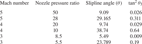
  $\tan ^2 \theta _3$ in (4.2g) can be neglected, and the slipline can be modelled as given in (4.3). Table 2 shows the slipline angle and the value of the
  $\tan ^2\theta _3$ for different Mach numbers and NPR for the overexpanded jet. The slipline angles and corresponding
  $\tan ^2\theta _3$ values are larger for lower NPR than the higher NPR for all Mach numbers. Similar results are reported in Bai & Wu (Reference Bai and Wu2017) for supersonic wedge flows with higher Mach numbers compared with the lower Mach number flows.

Figure 6. Comparison of analytical methods for various Mach numbers and NPR. The analytical results are compared with the Li & Ben-Dor (Reference Li and Ben-Dor1997b) model.
Table 2. Six different cases of the overexpanded jet with different Mach numbers and NPR showing the slipline angle and the value of the ignored term in the modelling of Li & Ben-Dor (Reference Li and Ben-Dor1997b).
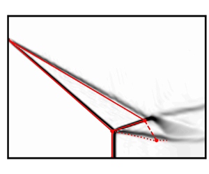
The comparison of analytical estimates of the Mach stem height using the modified Li and Ben-Dor model, Mouton and Hornung model and the Bai and Wu model for the overexpanded jets is shown in figure 7. All the analytical models predict the theoretical von Neumann condition where the Mach stem height goes to zero, precisely for all the Mach numbers. The modified Li and Ben-Dor model and the Mouton and Hornung model predict identical values for the Mach stem height at higher NPR and the deviation increases as the NPR is decreased. The maximum deviation between the two models occurs at NPR closer to the sonic condition behind the reflected shockwave where the jet is highly overexpanded. The critical difference between the models that are seen in figure 7 is that the Li and Ben-Dor method overestimates the Mach stem height at higher Mach numbers than the Mouton and Hornung method, while the trend is reversed at lower Mach numbers. The prediction of the Mach stem height by the analytical model in the overexpanded jet contradicts that in wedge flows. It is reported in Bai & Wu (Reference Bai and Wu2017) that the Mach stem height estimate by the Mouton & Hornung (Reference Mouton and Hornung2007) model for the wedge flow is higher than the Li & Ben-Dor (Reference Li and Ben-Dor1997a) for higher Mach number, and the trend reverses for the lower Mach number flows. The exact reason for this discrepancy may be attributed to the modelling of the slipline, as the two models differ entirely in this regard. For the case of the Bai and Wu model, the trend in estimating the Mach stem height departs considerably from the other methods discussed above, as can be seen in the wedge flows for the Bai & Wu (Reference Bai and Wu2017) model as well. It is worth noting that the increased complexity in modelling the flow field adjacent to the slipline and accounting for all the significant wave interactions happening over the slipline makes the Bai and Wu model challenging to solve numerically compared with the other models. As a result, the Bai and Wu model for the overexpanded jet could not predict the Mach stem height for highly over-expanded conditions (lower NPR) of the open jet. The comparison of the computational data against the analytical results is shown in figure 7. In the numerical solution, the Mach stem height is estimated as the distance from the triple point ( $T$) to the foot of the Mach stem. The triple point is assigned to the point where the three shocks meet along with the slipline. The error associated with the triple point location is at least three cells wide in the
  $y$ direction, and the error related to the nozzle exit height is at least one cell wide in the
  $y$ direction. The error bars are calculated based on the
  $\Delta y$-cell width value obtained from the grids. The difference between the numerical and analytical values of the von Neumann condition is substantial, and the numerical value is always lower than the analytical value, as seen in figure 7. The possible reason for this discrepancy is that the Mach stem height rapidly reduces to zero as the NPR increases towards the von Neumann condition in the numerical simulations than the analytical model does. This could be attributed to several aspects. The most critical element is the Kelvin–Helmholtz instability developed in the slipline that interacts with the symmetry boundary conditions at higher NPR where the Mach stem height is small. The grid resolution and NPR step size are other significant factors affecting the proper identification of the von Neumann condition. As the Mach stem gets smaller, even for a sufficiently refined grid, the transition happens before the theoretical value of the von Neumann condition in the flow field. For the present computations, the transition of the MR to RR configuration is checked for successively refined grids and different NPR step sizes of 0.1, 0.05, 0.01. Despite refining the grid and reducing the NPR step size considerably, the resulting numerical simulations did not alter the NPR required for the transition from MR to RR configuration, confirming that the NPR step size and the grid resolution does not impact the transition criterion. The inability of the successively refined grids and NPR step size to explain the sudden transition makes the problem interesting for further study and to understand the discrepancy seen in the numerical simulations. For a range of NPRs sufficiently away from the von Neumann condition, the Mach stem height agreement is excellent for higher Mach numbers and reasonably accurate for lower Mach numbers. The significant difference in the models comes mainly from the modelling of the slipline in the flow field. In the Mouton and Hornung method, the slipline is assumed to be an inviscid wall, and the pressure discontinuity across the slipline is allowed. Thus, the slipline's curvature, which can affect the subsonic portion and the sonic point location, is not considered. In the Li and Ben-Dor method, the curvature created by the expansion fan interaction is modelled to estimate the Mach stem height. The modelling of the curvature plays an essential role in the proper estimation of the Mach stem height. As a result, the Bai and Wu method, which includes complex wave interactions modelled over the slipline as the flow in the subsonic duct accelerates, gives the best possible estimate for the Mach stem height. From the numerical simulation results, it is seen that for highly overexpanded conditions and higher Mach numbers, the slipline generated is almost straight, and the Mouton and Hornung method gives good results, while for the lower Mach number, the Li and Ben-Dor results match very well, which ascertains the importance of proper modelling of the curvature of the slipline in the flow field.

Figure 7. Comparison of Mach stem height predicted by the analytical models and computational fluid dynamics (CFD) results for various Mach number and NPR: (a)  $M = 5$; (b)
  $M = 4$; (c)
  $M=3$; (d)
  $M = 2.75$.
7.2. Comparison of analytically and computationally predicted flow fields
The results obtained from the analytical methods developed for the overexpanded jets give the overall configuration of the MR in the flow field, i.e. incident shock ( $i$), reflected shock (
 $r$), Mach stem (
 $m$), triple point (
 $T$), slipline (
 $s$), along with the expansion fan from the jet boundary. The locations of the discontinuities obtained from the analytical results for an open jet corresponding to
  $M = 5$ and
  ${\rm NPR} = 50$ are superimposed on the numerical schlieren obtained from the density gradient computed from the MR solution for the inviscid simulation for the same conditions are shown in figures 8 and 9. The density gradient is then transformed to an exponential scale using the method proposed by Quirk (Reference Quirk1997).

Figure 8. Comparison of the position of the geometric quantities obtained from the analytical results for both the methods superimposed on the numerical schlieren solutions for  $M = 5$ and
  ${\rm NPR} = 50$ overexpanded jet.

Figure 9. Comparison of the position of geometric quantities obtained from Bai and Wu's method superimposed on the numerical schlieren solution for  $M = 5$ and
  ${\rm NPR} = 50$ jet.
The overlay of the geometric quantities such as incident shock wave, jet boundary and the Mach stem from the Li and Ben-Dor method, and the Mouton and Hornung method, deviates considerably from the numerical results as seen in figure 8. For the Bai and Wu method shown in figure 9, the locations of the incident shockwave, jet boundary and the Mach stem agree reasonably well with the numerical results, and this method models the jet much more accurately than other analytical models. The foot of the Mach stem is taken to the same  $x$ location as that of the triple point for all the analytical models. The locations of reflected shock and the subsequent expansion fan interaction with the slipline differ considerably from the numerical results for all the analytical models, including the Bai and Wu model, which gives the closest estimate for the Mach stem height obtained from the numerical simulation. Despite the difference in resolving the positions of the reflected shock wave, expansion fan and the slipline by the analytical modelling compared with the computational results, the Mach stem height is estimated very well for the given conditions, especially in the case of the Bai and Wu model. For the other two analytical models, the trend of the Mach stem height variation with the NPR matches the numerical data until the deviation occurs close to the von Neumann condition.
7.3. Comparison of experimental results with the analytical model
The validity of the analytical models to estimate the Mach stem height is verified using Mach stem height measurements from the experiments. The Mach stem height is measured from the schlieren images obtained from the experiment for various NPRs in the overexpanded jets based on the calibration of the images. The details of the calibration and the error estimates are given in Appendix C.
The calculated non-dimensional Mach stem height is plotted with the numerical and the analytical results and shown in figure 10. The experimental measurement of the non-dimensional Mach stem height over predicts the computational results, as shown in figure 10. The experimental result matches the Mouton and Hornung method reasonably well compared with the Li and Ben-Dor method and Bai and Wu method, whereas the numerical results match the Li and Ben-Dor results at lower NPRs. The Bai and Wu method results deviate from other methods and match the numerical results at higher NPR, i.e. closer to the von Neumann condition. The Bai and Wu method could not predict any Mach stem height for lower NPR due to the numerical issues discussed earlier, whereas other analytical models predict Mach stem height at all NPR. The experimental results deviate considerably from the numerical and analytical results for lower NPR close to the second critical pressure. The deviation of the Mach stem at the lower NPR may be due to the viscous effects and the turbulent nature of the jet interacting with the shock waves in the shock cell. The reason for the dominance of the viscous force/turbulence effect is that the flow from an actual nozzle undergoes shock-induced separation from the nozzle walls at pressure ratios smaller than the second critical pressure, and thus an MR structure is usually formed inside the nozzle instead of a planar normal shock. As the NPR increases, the MR structure moves downstream beyond the second critical pressure ratio. The Mach stem height as it comes out may be considerably different from the analytical and the inviscid computational solutions. Once the MR structure comes out and the NPR is sufficiently large enough where the separated region in the nozzle vanishes, the MR closely follows the inviscid calculations. Hence, the Mach reflection configuration and the Mach stem height match acceptably well with the inviscid model of analytical methods and experimental results for sufficiently high NPR.

Figure 10. Comparison of experimental and numerical results of Mach stem height for  $M = 2.44$ overexpanded jet with the analytical models.
7.4. Comparison of open jet shock reflections with the wedge flows
The Mach reflection configuration in the open jet shows subtle differences and similarities with the wedge flows. The analytical method developed to estimate the height of the Mach stem, models the entire MR configuration and provides the insight to understand the differences that arise from these configurations. All the analytical models yield similar results, and for the sake of brevity, the modified Li and Ben-Dor model is used to describe the qualitative differences observed in the flow field. The analytical results for both the flows are obtained by keeping the critical non-dimensional parameters such as wedge length ( $w/H$), jet boundary length and Mach number constant for various NPR and the equivalent wedge angles. The comparison between these flows is shown in figure 11, where the non-dimensionalised Mach stem height is plotted against the wedge angle/jet boundary angle for a Mach number
  $M = 5$ jet. From the modelling point of view, the flow field and the shock structure between the two flows are identical if the non-dimensional parameters are kept constant. This is one of the limiting cases in the wedge flows where the reflected shockwave hits the trailing corner of the wedge. The similarity between the MR configurations for the two flow fields result in the identical Mach stem height from two algorithms, as seen in figure 11. This exact agreement between the Mach stem height in the wedge and open jet flows shows the reliability of the modified model to effectively predict Mach stem height and describe the flow field accurately. The significant difference in the MR configuration in these flows is shown in figure 12, where the non-dimensional Mach stem height is plotted against the wedge angle and the corresponding NPR for the wedge flows and overexpanded jets, respectively. In figure 12, the wedge length, i.e.
  $w/H$, is kept constant while the wedge angle is changed continuously, which results in different MR configurations. The non-dimensionalised Mach stem heights are plotted for different
  $w/H$ ratios, and the Mach stem heights deviate substantially from the overexpanded jets. In contrast to the wedge flows where the Mach stem height depends on the physical lengths present in the flow field, i.e. wedge length, the Mach stem height in overexpanded jets do not depend on any geometrical parameter other than the nozzle exit height and thus can have a stable MR configuration for all the NPR ratios above the von Neumann condition as depicted in figure 12. All the curves for the wedge flow terminate at the overexpanded jet curve, which essentially represents the upper bound of the Mach stem height attainable by the wedge flows for any configuration. Moreover, the size of the Mach stem can change drastically for a given wedge angle and Mach number based on the
  $w/H$ ratio, and the MR configuration can be unstable for certain wedge angles depending on the
  $w/H$ ratio. Li & Ben-Dor (Reference Li and Ben-Dor1997a) provided an analytical expression to calculate the unstable regimes in the MR configuration domain as
  $H_{t,max}$ and
  $H_{t,min}$, where
  $H_t$ is the distance from the wedge trailing edge corner to the symmetry line. If the
  $H_t$ exceeds either of these values, i.e.
  $H_{t,min}$ and
  $H_{t,max}$ then the MR is unstable, and the entire configuration will go either to the unstart condition or may change to RR depending on the interaction of the expansion waves with the triple point. The overexpanded jet represents the limiting case of
  $H_{t,min}$ for the wedge flows and thus depicts the maximum possible Mach stem height for the wedge flows. The absence of length scales in the open jets results in the linear growth of the Mach stem height with the nozzle exit height. The Mach stem height slope also changes remarkably, i.e. from concave nature for the overexpanded jet to convex nature for the wedge flows.

Figure 11. Comparison of Mach stem height for the wedge flow and the overexpanded jet for  $M = 5$. To compare the open jet flow with the wedge flow, the wedge length is changed for every wedge angle to match the jet boundary length in the open jet.

Figure 12. Comparison of Mach stem height for overexpanded jet and wedge flow using modified Li and Ben-Dor method and Li & Ben-Dor (Reference Li and Ben-Dor1997a), respectively, for various  $w/H$ ratios along with the
  $H_{t,max}$ and
  $H_{t,min}$ values.
7.5. Mach stem growth rate prediction in open jets
The formation/appearance of the Mach stem in the dual solution domain (Ben-Dor Reference Ben-Dor2007) as part of the RR–MR transition due to the upstream disturbance in the flow field can be modelled using the analytical methods developed for the open jets. The growth of the Mach stem during the  $RR \longrightarrow MR$ transition is an extremely small time scale phenomenon and can be predicted by extending the analytical models developed by Mouton & Hornung (Reference Mouton and Hornung2007) and Li, Gao & Wu (Reference Li, Gao and Wu2011) for the wedge flows. A summary of the algorithm to estimate the Mach stem growth rates in the overexpanded jets is described below. The algorithm involves transforming the coordinates to the triple point and solving the three-shock theory based on the motion of the triple point. The coordinate system travels with the triple point along with the incident shockwave with speed
  $U_T$. The velocity components measured from the triple point coordinates are used to compute the flow field in the vicinity of the triple point using the equations described in Li et al. (Reference Li, Gao and Wu2011). Once the flow field closer to the triple point is obtained, the Mach stem height is calculated similarly to any of the algorithms described in § 3. In the present study, the modified Li and Ben-Dor method is used to estimate the growth rate of the Mach stem in the flow field. The Mach stem growth rate results are shown in figure 13. The plots show the non-dimensional time and the non-dimensional velocity against the non-dimensional Mach stem height. The non-dimensionalisation is carried out using the reference quantities, i.e. the sound speed at the exit of the nozzle (
 $a_c$).

Figure 13. (a) Mach stem growth rate and (b) triple point velocity variation is plotted for open jet of  $M=5$ and
  ${\rm NPR}=45.81$ and corresponding wedge flow of
  $M=5$ and
  $\theta =27.8^{\circ }$.
The variation of the Mach stem height as time progresses is shown in figure 13(a) for the open jet and the wedge flow of similar conditions, i.e. Mach number  $M = 5$, flow deflection angle
  $\theta = 27.77$, wedge length of
  $w/H = 1.28$ which is equal to the jet boundary length. Figure 13(a) also shows the Mach stem growth for another wedge length
  $w/H =1.0$ to highlight the difference in the wedge flow. The growth rate of the Mach stem is similar for both the flows at initial times and the growth rate increases for the open jets and attains the steady state value at an earlier time when compared with the wedge flow with identical flow parameters. The Mach stem in the wedge flow grows slowly and follows a different path to attain the same steady state value as that of the open jet. Despite the identical flow parameters, the growth of the Mach stem is affected by the reflected shockwave and expansion fan interaction in the wedge flows. Similar interaction would be absent in the open jets, and the flow structure evolves without any geometrical dependence on the flow field. At any time instant, the MR structure of the open jet will correspond to the MR configuration in the wedge flows that gives the maximum value of the Mach stem height at that condition, i.e. for the jet boundary length corresponding to the same wedge length. At the steady state, the open jet gives the highest possible Mach stem height. Any wedge length smaller than the jet boundary length will follow the open jet growth rate at initial times and the Mach stem growth rate deviates and settles to a steady state value at longer times. From figure 13(a), it can be observed that the wedge flow takes a longer time to achieve the steady state value of the Mach stem compared with the open jet. This shows the geometrical dependence of the wedge flows in the Mach stem growth rate. Figure 13(b) shows the comparison of the non-dimensional triple point velocity as a function of the Mach stem height for open jets and the wedge flows. The plot shows that the non-dimensionalised velocity is maximum for the open jet when compared with the wedge flows at any given instant. If the wedge length is changed from that of the jet boundary length, the non-dimensional velocity changes drastically as the Mach stem grows. The triple point velocity is almost linear for the case of the open jets when compared with the wedge flows.
7.6. Effect of stagnation pressure and ambient pressure
The numerical simulations are carried out to study the effect of the stagnation pressure change ( $p_{stag}$) versus the ambient/backpressure change (
 $p_{amb}$) on the formation of MR and the transition to the RR in the flow field. The effect of back pressure and the stagnation pressure change is studied by fixing the stagnation pressure or the ambient pressure at a particular value, and the flow quantities at the exit plane of the nozzle are calculated based on the NPR. The numerical simulation of fixing the back/ambient pressure at a specific value corresponding to 1.01325 bar results in the simulations where the stagnation pressure changes continuously as the NPR is changed along with the jet exit pressure and the density. The stagnation pressure change increases the mass flow rate through the nozzle as the NPR is raised from the MR regime to the RR regime and decreases the mass flow rate as the NPR is reduced from the RR regime to the MR regime. The numerical simulation of fixing the stagnation pressure at a particular value and slowly decreasing the backpressure of the system will result in a constant mass flow rate at the exit plane and the constant flow properties of the jet at the exit plane of the nozzle. The results from the simulations are almost the same indicating that the Mach stem height does not depend exclusively on the stagnation pressure or backpressure, rather it depends only on the NPR.

Figure 14. Comparison of Mach stem heights obtained for various NPR by separately increasing the stagnation pressure and decreasing the backpressure for  $M=5$ jet.
7.7. Hysteresis in the overexpanded jets
The flow structures in the open jet exhibit a hysteresis phenomenon as the NPR is changed continuously during its operation. The Mach reflection at the exit of the nozzle for lower NPR should transit to RR at the detachment condition. However, in the strong deflection domain, the transition from MR to RR follows the von Neumann condition; hence, there is a small NPR range where both the MR and RR solutions are possible for the same NPR. This regime is called a dual solution regime (Landau & Lifshitz Reference Landau and Lifshitz1987). The existence of a dual solution regime in the 2-D overexpanded jet was showed by Hadjadj et al. (Reference Hadjadj, Kudryavtsev and Ivanov2004) for  $M = 5$ jets. Figure 15 shows the Mach stem height as a function of NPR for two different processes (i.e. increasing NPR and decreasing NPR) corresponding to MR–RR transition and RR–MR transition in the open jet for four different Mach numbers. From figure 15, it can be seen that both a finite and a zero Mach stem height, i.e. MR and RR solutions for the same NPR. This indicates the presence of the hysteresis loop in the overexpanded jet for various Mach numbers. The hysteresis loop is also observed when the backpressure is changed continuously instead of the stagnation pressure to achieve the different NPR values, as seen in figure 16. The shock polar solution and the resulting change in the pressure behind the flow field are shown in figure 17. The RR solution represents the higher pressure jump in the flow field rather than the MR solution in the dual domain solution. Figure 18 shows the presence of hysteresis in the
  $M = 5$ jets for various NPR. Figure 18(a–c), show the numerical schlieren of MR configurations in the dual solution regime. The flow fields shown in figure 18(a–c) are obtained by continuously increasing the NPR from the MR regime beyond the detachment condition. The MR configuration persists as the NPR is increased further, and the transition to RR happens close to the von Neumann condition. Figure 18(d–f) show the numerical schlieren with the RR configuration in the dual solution domain. The numerical solution corresponding to the RR solution in the dual domain is obtained by RR as the initial condition, and the NPR is decreased gradually. The RR solution now persists as the NPR crosses the von Neumann condition. This shows the dual solution domain in the open jets. When the NPR reaches the value of the detachment condition, the Mach stem suddenly appears in the flow field, which changes the flow field drastically.

Figure 15. Presence of dual-domain solution and the hysteresis of the MR–RR shock structure for various Mach numbers as the NPR is varied continuously: (a)  $M = 5$; (b)
  $M = 4$; (c)
  $M = 3$; (d)
  $M = 2.75$.

Figure 16. Mach stem height versus the NPR ratio for  $M=5$ overexpanded jet. The increase and the subsequent reduction of the back pressure show the hysteresis in the shock reflections in the jet.

Figure 17. Dual solution regime for  $M=5$ and
  ${\rm NPR}=49.5$ overexpanded jet: (a) shock polar solution; (b) centreline pressure distribution.

Figure 18. Numerical schlieren of  $M=5$ overexpanded jet showing the MR and RR configuration for the same NPR. Panels (a,c,e) show the MR configuration, panels (b,d,f) show the RR configuration and panel (g) shows the RR configuation outside the von Nuemann condition.

Figure 19. Schematic of the computational domain and the boundary condition for the overexpanded jet simulations.
8. Conclusions
The analytical formulation of the Mach stem height in the wedge flows by Li & Ben-Dor (Reference Li and Ben-Dor1997a), Mouton & Hornung (Reference Mouton and Hornung2007) and Bai & Wu (Reference Bai and Wu2017) methods are successfully extended to the overexpanded jet problem. The high-order numerical simulations of the overexpanded jet show excellent agreement with the Bai and Wu method for all Mach numbers and NPR where the algorithm gives the solution. The experimental results for the  $M = 2.44$ overexpanded jet show a reasonable agreement with the inviscid formulation of the analytical and numerical estimations of Mach stem height. The viscous effects and the lateral expansion of the jet in the experiments play a significant role in the highly overexpanded jets conditions, leading to the deviation of the analytical and numerical values from the experimental results. It has been found that the Mach stem height in the open jet is the upper bound for any attainable Mach stem height in the corresponding wedge flow. The open jet also shows a unique Mach reflection configuration for the given conditions while wedge flows are dependent on the geometry of the wedge, i.e.
  ${w}/{H}$ value. The growth rate of the Mach stem in the open jets during the transformation from regular reflection is greater than the corresponding wedge flows. Despite the same Mach stem height at the steady state conditions for wedge and open jet flows, the growth rate is affected by the interaction of the reflected shockwave with the expansion fan in the wedge flows. The analytical model also shows that the growth rate changes drastically as the geometry of the wedge is changed as expected from the Mach stem height deviation. Further numerical studies are needed to verify the analytical growth rate predictions in the open jet.
The present methods for estimating Mach stem height work well only in the regime where the flow behind the reflected shock is supersonic, i.e. only in the strong shock reflection domain. Future work will involve extending the above method to the weak Mach reflection domain in the overexpanded jets and estimating Mach stem height in the underexpanded jets. The effect of viscous flow computation on the Mach stem and the hysteresis formation can also be studied along with the turbulence modelling on estimating the Mach stem height.
Acknowledgements
We acknowledge the use of the computing resources at HPCE, IIT Madras.
Declaration of interests
The authors report no conflict of interest.
Appendix A. Three shock theory and isentropic relations
The solution of Mach stem height starts with obtaining a solution close to the triple point. To solve the flow field near the triple point, the conservation equations/oblique shock relations are solved with the appropriate boundary conditions (i.e. the solution to the three shock theory of von Neumann). These equations relate density, pressure, temperature, Mach number and flow deflection angle ( $\theta$) behind an oblique shockwave as a function of incident Mach number (
 $M$) and shockwave angle (
 $\beta$). The oblique shock relations are applied across incident (
 $I$), reflected shockwave (
 $R$) and Mach stem (
 $m$) as follows:
(i) Mach number relation
(A1)\begin{equation} M_j=\sqrt{\frac{\left(1+(\gamma-1)M_i^2\sin^2\beta_i+\left[\dfrac{(\gamma+1)^2}{4}-\gamma \sin^2\beta_i\right]M_i^4\sin^2\beta_i\right)}{\left[\gamma M_i^2\sin^2\beta_i-\dfrac{\gamma-1}{2}\right]\left[\dfrac{\gamma-1}{2}M_i^2\sin^2\beta_i+1\right]}}; \end{equation}(ii)
$\theta -\beta -M$ relation
(A2)\begin{equation} \theta_i=\arctan\left[2\cot\beta\frac{M_i^2\sin^2\beta_i-1}{M_i^2(\gamma+\cos2\beta_i)+2}\right]; \end{equation}(iii) pressure relation
(A3)\begin{equation} p_j=p_i\frac{2}{\gamma+1}\left[\gamma M_i^2\sin^2\beta_i - \frac{\gamma-1}{2}\right]; \end{equation}(iv) density relation
(A4)\begin{equation} \rho_j=\rho_i\frac{(\gamma+1)M_i^2\sin^2\beta_i}{(\gamma-1)M_i^2\sin^2\beta_i+2}; \end{equation}(v) temperature relation
(A5)where i and j denote the upstream and downstream conditions across the oblique shockwave, respectively. These form a set of 15 equations with 17 unknowns. To complete the above set of equations, boundary conditions and pressure equilibrium conditions across the slip line are used. Once the equations are solved, the flow field near the triple point is obtained.\begin{equation} T_j=T_i\frac{[(\gamma-1)M_i^2\sin^2\beta_i+2][2\gamma M_i^2\sin^2\beta_i-(\gamma-1)]}{(\gamma+1)^2M_i^2\sin^2\beta_i}, \end{equation}(vi) Boundary condition and pressure equilibrium conditions,
(A6)$$\begin{gather} p_2=p_3, \end{gather}$$(A7)In the present computations, only strong shock interactions are considered and hence the use of (A7) for the boundary condition. The solution to the above equations gives the complete information about the flow field closer to the triple point$$\begin{gather}\theta_1-\theta_2=\theta_3. \end{gather}$$$T$. For solving the expansion fan region, various isentropic relations are used. The amount of flow deflection needed for the expansion fan to make the flow parallel behind the reflected shock is calculated using the isentropic relations and Prandtl–Meyer relations for the expansion fan. Equations (A8)–(A10) describe these relations, as follows:
(A8)$$\begin{gather} \nu(M_D)=\sqrt{\frac{\gamma+1}{\gamma-1}}\arctan\sqrt{\frac{\gamma-1}{\gamma+1}(M_D^2-1)}-\arctan\sqrt{M_D^2-1} , \end{gather}$$(A9)$$\begin{gather}\nu(M_D)=\nu(M_2)+\theta_3, \end{gather}$$(A10)where$$\begin{gather}\frac{p_i}{p_j}=\left(\frac{1+\dfrac{\gamma-1}{2}M_j^2}{1+\dfrac{\gamma-1}{2}M_j^2}\right)^{{\gamma}/({\gamma-1})}, \end{gather}$$$M_D$ is the Mach number upstream of the expansion wave where the flow will be parallel to the symmetric line. Here $M_2$ is the Mach number behind the reflected shockwave and $\theta _3$ is the slip line angle at the triple point. Equation (A10) is the isentropic relation for the pressure ratio at two different points in a streamline.


Appendix B. WENO-ZQ formulation
The WENO schemes are widely used in the computations that contain strong shocks in the flow fields. These methods can capture shocks in the flow field without any oscillations and also provide a higher order of accuracy by adaptively choosing the stencils to reconstruct the flow variables at the cell face. The robustness and the non-oscillatory property make the WENO reconstruction ideal for simulations of overexpanded jets that contain strong shock interactions in the flow field. In the WENO-ZQ reconstruction, a fourth-degree polynomial, i.e. a fifth-order reconstruction, is carried out using the central stencil that involves all the cells in the stencil and two linear polynomials, i.e. second-order reconstruction is calculated. The polynomials and the nonlinear weights used in the present formulation are given below. These formulations can be obtained from Zhu & Qiu (Reference Zhu and Qiu2017). Once the polynomials and the weights are evaluated, the final reconstructed value at the cell face can be obtained using equation (B7),
 \begin{gather}\hspace{-100pt} p_1(x)
= q_i+\frac{-82q_{i-1}+11q_{i-2}+82q_{i+1}-11q_{i+2}}{120}\left(\frac{x-x_i}{h}\right) \nonumber\\
\hspace{-50pt} +\,\frac{40q_{i-1}-3q_{i-2}-74q_i+40q_{i+1}-3q_{i+2}}{56}\left(\left(\frac{x-x_i}{h}\right)^2-\frac{1}{12}\right) \nonumber\\
\hspace{-55pt} +\,\frac{2q_{i-1}-q_{i-2}-2q_{i+1}+q_{i+2}}{12}\left(\left(\frac{x-x_i}{h}\right)^3-\frac{3}{20}\left(\frac{x-x_i}{h}\right)\right) \nonumber\\
\hspace{30pt} +\,\frac{-4q_{i-1}+q_{i-2}+6q_{i}-4q_{i+1}+q_{i+2}}{24}\left(\left(\frac{x-x_i}{h}\right)^4-\frac{3}{14}\left(\frac{x-x_i}{h}\right)^2-\frac{3}{560}\right),
\end{gather}
\begin{gather}\hspace{-100pt} p_1(x)
= q_i+\frac{-82q_{i-1}+11q_{i-2}+82q_{i+1}-11q_{i+2}}{120}\left(\frac{x-x_i}{h}\right) \nonumber\\
\hspace{-50pt} +\,\frac{40q_{i-1}-3q_{i-2}-74q_i+40q_{i+1}-3q_{i+2}}{56}\left(\left(\frac{x-x_i}{h}\right)^2-\frac{1}{12}\right) \nonumber\\
\hspace{-55pt} +\,\frac{2q_{i-1}-q_{i-2}-2q_{i+1}+q_{i+2}}{12}\left(\left(\frac{x-x_i}{h}\right)^3-\frac{3}{20}\left(\frac{x-x_i}{h}\right)\right) \nonumber\\
\hspace{30pt} +\,\frac{-4q_{i-1}+q_{i-2}+6q_{i}-4q_{i+1}+q_{i+2}}{24}\left(\left(\frac{x-x_i}{h}\right)^4-\frac{3}{14}\left(\frac{x-x_i}{h}\right)^2-\frac{3}{560}\right),
\end{gather} \begin{gather} p_2(x)=q_i+(q_i-q_{i-1})\frac{x-x_i}{h}, \end{gather}
 \begin{gather} p_3(x)=q_i+(q_{i+1}-q_i)\frac{x-x_i}{h}. \end{gather}
Smoothness indicators:
 \begin{gather} \beta_1
= \frac{1}{144}(q_{i-2}-8q_{i-1}+8q_{i+1}-q_{i+2})^2 \nonumber\\
\hspace{6.5pc} +\,\frac{1}{15600}({-}11q_{i-2}+17q_{i-1}-32q_i+174q_{i+1})^2 \nonumber\\
\hspace{4pc} +\,\frac{781}{2880}({-}q_{i-2}+2q_{i-1}-2q_{i+1}+q_{i+2})^2 \nonumber\\
\hspace{8.5pc} +\,\frac{1421461}{1310400}(q_{i-2}-4q_{i-1}+6q_i-4q_{i+1}+q_{i+2})^2,
\end{gather}
\begin{gather} \beta_1
= \frac{1}{144}(q_{i-2}-8q_{i-1}+8q_{i+1}-q_{i+2})^2 \nonumber\\
\hspace{6.5pc} +\,\frac{1}{15600}({-}11q_{i-2}+17q_{i-1}-32q_i+174q_{i+1})^2 \nonumber\\
\hspace{4pc} +\,\frac{781}{2880}({-}q_{i-2}+2q_{i-1}-2q_{i+1}+q_{i+2})^2 \nonumber\\
\hspace{8.5pc} +\,\frac{1421461}{1310400}(q_{i-2}-4q_{i-1}+6q_i-4q_{i+1}+q_{i+2})^2,
\end{gather} \begin{gather} \beta_2=(q_{i-1}-q_i)^2, \end{gather}
 \begin{gather} \beta_3=(q_i-q_{i+1})^2. \end{gather}
Reconstruction at the face:
 \begin{align} q_{i+{1}/{2}}^+&=\omega_1\left(\frac{1}{\gamma_1}p_1\left(x_{i+{1}/{2}}\right)-\frac{\gamma_2}{\gamma_1} p_2\left(x_{i+{1}/{2}}\right)-\frac{\gamma_3}{\gamma_1}p_3\left(x_{i+{1}/{2}}\right)\right)\nonumber\\ &\quad +\omega_2p_2\left(x_{i+{1}/{2}}+\omega_3p_3\left(x_{i+{1}/{2}}\right)\right) , \end{align}
where  $q$ represents the characteristic variable,
  $\beta$ represents the smooth indicators for the polynomial reconstruction,
  $\gamma$ represents the linear weights and
  $\omega$ represents the nonlinear weights. The definition of the nonlinear weights can be found in Zhu & Qiu (Reference Zhu and Qiu2017). The computational domain for the present simulation is given here in figure 19.
Appendix C. Calibration and error estimation in schlieren images
The calibration of the image is carried in the following manner. The exit of the jet occupies approximately 180 pixels in length in the schlieren image. These 180 pixels correspond to 50 mm, which translates 1 pixel to 0.278 mm in dimension. The calibrated value of the pixel converts the Mach stem height measured in pixels to physical length in millimetres. The error in the measurement of the Mach stem height and the exit length of the nozzle is given in terms of the pixels. The pixel error in measuring the nozzle exit is two pixels wide, and the error in measuring the Mach stem height is six pixels, i.e. at most of six pixels in locating the triple point location. Hence the total error in estimating the non-dimensional Mach stem height is given in (C1) where  $Z$ and
  $\Delta Z$ represent the non-dimensionalised Mach stem height and the associated error,
  $A$ and
  $B$ represent the Mach stem height and the nozzle exit height and
  $\Delta A$ and
  $\Delta B$ represent the error in the measurements of
  $A$ and
  $B$, respectively; then, the error associated with the
  $Z$ is given by (C2),
 $$\begin{gather} Z=\frac{A}{B}, \end{gather}$$
 $$\begin{gather}\Delta Z=\frac{1}{B}\sqrt{\Delta A^2+Z^2.\Delta B^2}. \end{gather}$$


 Open access