


1. Introduction
Bluff-bodies are often porous or perforated in applied scenarios. Perforated bodies find application in the process of aggregation, sedimentation and filtration (e.g. design of industrial gauzes and flue exhaust systems). They are also utilized in electronic cooling systems, multi-jet burners, grated decks and fences (Kim & Lee Reference Kim and Lee2002). In addition, Sha & Launder (Reference Sha and Launder1979) modelled pipe bundles as porous bluff-body wakes. More recently, perforated bodies have been used to model wind turbine wake phenomena (Xiao et al. Reference Xiao, Duan, Sui and Rosgen2013; Steiros & Hultmark Reference Steiros and Hultmark2018).
The earliest work in this subject was carried out by Taylor (Reference Taylor1944), who studied the wake from perforated flat plates. Following Taylor (Reference Taylor1944), some attempts have been made to investigate this problem. However, the most comprehensive study has been reported by Castro (Reference Castro1971). In his study, flow past perforated flat plates is classified into two regimes based on the porosity  $\beta$ (ratio of the open area to the total plate area). In the low porosity regime,
  $\beta < 20\,\%$, the ‘near’ wake was characterized by a dominant Kármán vortex street, which ceased to exist for higher
  $\beta$ (Castro Reference Castro1971). This regime change seems to be quite sudden at
  $\beta \approx 20\,\%$. Castro (Reference Castro1971) further reported abrupt changes in the measurements of drag coefficient
  $C_D$, Strouhal number
  $St$ and peak streamwise turbulence intensity
  $u_{rms}/U_\infty$ around this critical
  $\beta$. The limited literature available in this area further indicates that porosity alone is the dominant geometrical parameter characterizing this flow (Castro Reference Castro1971; Huang et al. Reference Huang, Ferré, Kawall and Keffer1995; Huang & Keffer Reference Huang and Keffer1996; Huang, Kawall & Keffer Reference Huang, Kawall and Keffer1996). In the study of flow over a perforated fence with different hole shapes, Perera (Reference Perera1981) found that the wake structure far downstream of the fence was affected mainly by the porosity, and was independent of the hole shape. In a recent study by Bae & Kim (Reference Bae and Kim2016), for a steady laminar wake they found drag coefficient dependence on both porosity and hole shape. It is therefore not clear why this regime shift occurs around 20 % porosity, and why porosity alone dominates the wake phenomenon.
The prior studies in this area further disagree with the reasons for strong periodicity in the ‘far’ wake of perforated bluff bodies of higher  $\beta$ (
 ${>}20\,\%$). Some suggest that the growth of large-scale unsteady structures in the ‘far’ wake is due to hydrodynamic instability of the mean flow in the absence of a vortex street (Castro Reference Castro1971; Cimbala, Nagib & Roshko Reference Cimbala, Nagib and Roshko1988). It is suggested that the two shear layers separated by the bleed flow coalesce some way downstream such that the wake becomes unstable and begins to ‘flap’. Here, it is said that there is just enough ‘bleed’ flow to prevent the formation of a vortex street. Others propose that the small-scale vortices in the formation region (i.e. near the body) merge to form quasi-periodic Kármán-like structures (Huang et al. Reference Huang, Ferré, Kawall and Keffer1995; Huang & Keffer Reference Huang and Keffer1996). The study by Wygnanski, Champagne & Marasli (Reference Wygnanski, Champagne and Marasli1986) also reported the phenomenon, but the reason for strong unsteadiness in their porous bluff-body wake is not apparent.
The critical transition Reynolds number  $Re_c$ for a non-perforated flat plate placed normal to the free stream is
  ${\approx }105\unicode{x2013}110$. According to Julien, Lasheras & Chomaz (Reference Julien, Lasheras and Chomaz2003), Julien, Ortiz & Chomaz (Reference Julien, Ortiz and Chomaz2004) and Thompson et al. (Reference Thompson, Hourigan, Ryan and Sheard2006), the route-to-transition in the wake of non-perforated flat plates takes place in two stages: first through a quasi-periodic mode of wavelength
  $\lambda = 5d\unicode{x2013}6d$ at
  $Re_c \approx 105\unicode{x2013}110$; and thereafter through mode A of wavelength
  $\lambda \approx 2d$ at
  $Re_c \approx 125$. Quasi-periodicity is the property of a system that displays irregular periodicity. In comparison, the circular cylinder wake becomes unstable to mode A at
  $Re\approx 190$, followed by bifurcation to mode B at
  $Re \approx 230\unicode{x2013}240$ (Williamson Reference Williamson1988). Here, mode A is characterized by an antisymmetric pattern of streamwise vortices from one braid region to the next, with wavelength
  ${\approx }4D$, where
  $D$ is the cylinder diameter; and mode B is defined as a secondary vortex structure with a symmetric pattern of streamwise vortices with wavelength
  ${\approx }1D$. At this stage, it is not clear how a transitional wake or a wake that is barely turbulent or experiencing transition-to-turbulence would respond to perforation (cf. table 1). The presence of perforation can further complicate the transition process since the jet of fluid emanating through the holes in the base region may affect the growth of secondary instabilities favourably or adversely.
Table 1. Flow over various perforated bodies. Here, superscripts  $^a$ and
  $^b$ refer to
  $Re$ based on hole and Taylor-microscale, respectively; Expt means experiment; Sim means simulation; DVM means discrete vortex method; LES means large-eddy simulation; RANS means Reynolds-averaged Navier–Stokes).

Further, the characteristics of the jet or the ‘bleed’ flow through the holes itself has received modest attention. Kim & Lee (Reference Kim and Lee2001, Reference Kim and Lee2002) in their experimental study of flow over a fence observed that for a given  $\beta$, hole size affects the upstream flow retardation and jet coalescence downstream of the body. The upstream flow retardation has been found to increase with reduction in hole size, while the jet coalescence and mixing increased with increase in hole dimension. This is reasonable since one can expect the jets to behave in an isolated fashion when the pitch separation
  $c$ between them is sufficiently large compared to the hole dimension
  $h$). On the contrary, if the pitch
  $c/h$ or the gap is sufficiently small, then the adjacent shear layers can experience proximity interference effects leading to engulfment or meandering oscillations and instabilities (Dadmarzi et al. Reference Dadmarzi, Narasimhamurthy, Andersson and Pettersen2018). Villermaux & Hopfinger (Reference Villermaux and Hopfinger1994) have reported a low-frequency (longitudinal) oscillation of the jet merging distance in their experimental study of co-flowing jets from a perforated body. To our knowledge, no other studies have explored this jet or ‘bleed’ flow characteristic and its immediate effect on the ‘near’-wake vortex dynamics of a perforated plate. Note that in addition to the co-flowing or neighbouring jets interaction, complex interference occurs also between the jets and the wake (shear layers emanating from the two edges of the plate), thus leading to jet–wake coupling.
Table 1 summarizes the literature concerning various studies of perforated bodies. Note that most of the perforated geometries were considered in an internal flow configuration. Barring Bae & Kim (Reference Bae and Kim2016), all the other studies have investigated high-Reynolds-number flows in the turbulent regime, and none exists on the ‘transitional’ or low-Reynolds-number turbulent regime. In addition, the problem has (unfortunately) received little attention from the numerical community (especially the direct and large-eddy simulation community). This, along with the concerns raised in the previous paragraphs, clearly demands a detailed investigation. We therefore aim to explore some of those mechanisms and the intricate flow physics through a direct numerical simulation (DNS) study; DNS as a scientific tool is the natural choice to probe such a complex wake phenomenon, since it enables complete access to the instantaneous three-dimensional data. With the aid of vortical structures, spectral analysis, spatio-temporal maps, and single- and multi-point statistics, we wish to disseminate answers to some of the open questions and also report new observations.
2. Problem definition and numerical details
In the current DNS study, the Reynolds number is set to  $Re_d = U_o d/\nu = 250$, where
  $U_o$ and
  $d$ refer to inflow velocity and plate width, respectively. This Reynolds number corresponds to the DNS study of a non-perforated flat plate wake by Najjar & Balachandar (Reference Najjar and Balachandar1998). Note that this
  $Re_d = 250$ is well above the critical transition Reynolds number (
 ${\approx }105\unicode{x2013}110$) for a non-perforated flat plate placed normal to the free stream.
The present set-up is shown in figure 1. Unless stated explicitly, all spatial dimensions are scaled by  $d$, and all velocity fields are normalized by
  $U_o$. Figure 1(b) shows the perforation pattern, where a plate of width
  $d$, thickness
  $0.02d$ and length
  $L_y = 6d$ is considered with six equidistantly spaced square holes arranged in an in-line fashion. Here,
  $c$ and
  $m$ refer to the pitch separation and the mid-gap between the holes, respectively. The porosity
  $\beta$ is determined through the hole dimension
  $h$ and number of holes
  $n$, i.e.
  $\beta = (n h^2/L_y d)\times 100\,\%$. In the present study,
  $\beta = 0\,\%$, 4 %, 9 %, 12.25 %, 16 %, 20.25 % and
  $25\,\%$ are considered (i.e. corresponding to
  $h/d = 0$, 0.2, 0.3, 0.35, 0.4, 0.45 and
  $0.5$, respectively). Note that the present plate thickness,
  $0.02d$, is same as that used in other numerical studies and is classified as ‘thin’ in the literature (Narasimhamurthy, Andersson & Pettersen Reference Narasimhamurthy, Andersson and Pettersen2008; Narasimhamurthy & Andersson Reference Narasimhamurthy and Andersson2009; Afgan et al. Reference Afgan, Benhamadouche, Han, Sagaut and Laurence2013; Choi & Yang Reference Choi and Yang2014; Tian et al. Reference Tian, Ong, Yang and Myrhaug2014; Hemmati, Wood & Martinuzzi Reference Hemmati, Wood and Martinuzzi2016; Dadmarzi et al. Reference Dadmarzi, Narasimhamurthy, Andersson and Pettersen2018). The length of the plate,
  $L_y = 6d$, is chosen based on a domain verification study (see Appendix B and also Singh & Narasimhamurthy Reference Singh and Narasimhamurthy2018, Reference Singh and Narasimhamurthy2021), where
  $L_y$ is varied from
  $1d$ to
  $12d$.

Figure 1. (a) Three-dimensional computational domain (not to scale). Here,  $x$ is the global streamwise coordinate, while
  $x'$ denotes the local streamwise coordinate with its origin at the plate location. (b) Side view depicting the perforated plate details.
Figure 1 shows the three-dimensional (3-D) computational domain, where  $L_x$,
  $L_z$ and
  $L_y$ denote streamwise, cross-stream and spanwise lengths, respectively. The plate is positioned at
  $5d$ downstream of the inflow. This domain is nearly the same as that used in other DNS studies of wake from non-perforated plates (cf. table 2 and Appendix B and C). The current mesh (
 $320 \times 240 \times 260$), however, is more refined than others, especially in the cross-stream (
 $N_z$) and spanwise (
 $N_y$) directions owing to the perforation pattern. The grid resolution around the plate is set as
  $[\varDelta _x,\varDelta _y,\varDelta _z] = [0.01,0.025,0.025]$. This numerical mesh is achieved based on a detailed grid verification test (see Appendix A and also Singh & Narasimhamurthy Reference Singh and Narasimhamurthy2021).
Table 2. Numerical mesh and domain details in various DNS studies of flow over normal flat plates. Here,  $L_{x_u}$ and
  $L_{x_d}$ refer to the upstream and downstream extents of the domain from the plate location, respectively, while
  $L_y$ and
  $L_z$ correspond to the spanwise and cross-stream lengths, respectively.

The incompressible Navier–Stokes equations are solved in 3-D space and time using the parallel finite volume code MGLET (Manhart Reference Manhart2004) with staggered Cartesian mesh. The spatial terms of the governing equations are discretized using a second-order central difference scheme, while the numerical solution is marched forward in time using a third-order explicit Runge–Kutta scheme. The Poisson equation is solved using the iterative strongly implicit procedure (SIP) method. A uniform velocity profile  $U_o$ (without any free stream perturbations) and a Neumann boundary condition for the pressure are prescribed as inflow. A free-slip condition is used on both top and bottom boundaries, while a periodic boundary condition is applied for the side boundaries (cf. figure 1). For outflow, a Neumann boundary condition is used for velocities and the pressure is set to zero. A direct forcing immersed boundary method (Peller et al. Reference Peller, Le Duc, Tremblay and Manhart2006; Narasimhamurthy et al. Reference Narasimhamurthy, Andersson and Pettersen2008) is used for converting the no-slip and impermeability boundary conditions on the plate into internal boundary conditions of the computational grid using a third-order-accurate least-squares interpolation scheme. A recent DNS study of wakes by Dadmarzi et al. (Reference Dadmarzi, Narasimhamurthy, Andersson and Pettersen2018) observed that initial conditions can alter significantly the final converged solution and thereby recreate many distinct states of flow reported independently in the literature. In the current study, therefore, all the simulations are started with the same initial conditions (a quiescent state). The time step is chosen as
  $\Delta t = 0.001 d/U_o$, and the number of Poisson iterations per time step is set to a maximum value of 60 (to achieve numerical residue
  $10^{-6}$). Parallelization is executed through a message passing interface (MPI). The simulations are run on an IBM System x iDataPlex dx360 M4 and a Dell PowerEdge R740 parallel computers. The wall clock times for
  $\beta = 0\,\%$, 4 %, 9 %, 12.25 %, 16 %, 20.25 % and 25 % are about 251, 827, 938, 718, 1397, 635 and 1137 h, respectively, with associated CPU times of about 16 046, 32 833, 60 038, 35 388, 89 433, 31 224, 72 757 h, respectively.
2.1. Flow past a non-perforated plate
As a reference case, flow over a non-perforated flat plate placed normal to the free stream is simulated, and the results are compared with the simulations of Najjar & Balachandar (Reference Najjar and Balachandar1998). Both two-dimensional (2-D) and three-dimensional (3-D) simulations are performed as the reference case (Najjar & Balachandar Reference Najjar and Balachandar1998). Figure 2 shows very good agreement of the mean pressure coefficient between the 2-D and 3-D cases, respectively. Here, the mean pressure coefficients on the front and back of the plate are defined as  $\bar {C}_{p,front} = ({\bar {p}_{front}-\bar {p}_{inlet}}) / ({0.5 \rho U_o^2})$ and
  $\bar {C}_{p,back} = ({\bar {p}_{back}-\bar {p}_{inlet}}) / ({0.5 \rho U_o^2})$, respectively, where
  $p$ is the pressure. Further, the mean drag coefficient
  $\overline {C_d}=({\bar {p}_{front}-\bar {p}_{back}}) / ({0.5 \rho U_o^2})$, and the Strouhal number
  $St_d=fd/U_o$, as given in table 3, show very good agreement between the simulations. Here,
  $f$ is the dominant frequency in the wake.

Figure 2. Mean pressure coefficient over a non-perforated plate at  $Re_d = 250$. Experimental data of Fage & Johansen (Reference Fage and Johansen1927) are at
  $Re_d = 1.5 \times 10^5$. The top and bottom halves of the curve signify the data from the front and back of the plate, respectively.
Table 3. Results from non-perforated plate simulations.

3. Results and discussions
In the present study, the instantaneous quantity  $\phi \in (u,v,w,p)$, recorded at a statistically stationary state, is decomposed into the time mean component
  $\bar {\phi }$ and the fluctuations
  $\hat \phi$. Here,
  $\hat \phi$ comprises both coherent and random motion.
3.1. Drag coefficient and Strouhal number
Figure 3 shows the dependence of the computed drag coefficient  $\overline {C_d}$, the blockage-corrected drag coefficient
  $\overline {C_{d_c}}$, and
  $St_d$ on
  $\beta$ (also reported in table 4). Here, the correction for the drag coefficient due to domain blockage was done using the method of Maskell (Reference Maskell1965) (see Appendix C for details). It is readily observed that there is excellent qualitative agreement with the experiments of Castro (Reference Castro1971) despite the large difference in
  $Re$ between the studies. Figure 3(a) shows the monotonic decrease in
  $\overline {C_d}$ with increasing
  $\beta$. However, its sharp fall is observed to be occurring much earlier than the
  $\beta \approx 20\,\%$ reported by Castro (Reference Castro1971). In the current DNS, an apparent reduction in drag is observed to start at
  $\beta \approx 4\,\%$. The exact location of the sudden drop cannot be determined due to a limited number of data points. Such a phenomenon arises because the vortex street formation region, where the separated shear layers begin to interact, is pushed further downstream as a result of the bleed flow through the plate (explained further in § 3.2). On the other hand, figure 3(b) shows that the increase in
  $St_d$ with respect to
  $\beta$ followed by a sudden drop at
  $\beta \approx 20\,\%$ is well predicted by the current DNS. Here, the blockage effect could have an influence on
  $St_d$ values reported in both studies. Note that the blockage ratio is almost the same in both studies. Additionally, the present DNS shows a higher
  $St_d$ as opposed to the experiments of Castro (Reference Castro1971). Such an increase in
  $St_d$ is attributed to a reduction in
  $Re_d$. Nevertheless, contrary to the observations of Castro (Reference Castro1971), it is quite interesting to observe that the sudden drop in
  $\overline {C_d}$ occurs at different
  $\beta$ in the present DNS, which could be an effect of the large difference in
  $Re$. Therefore, figure 3 demands further investigation to determine the mechanism for such a behaviour. Since the wake dynamics is believed to be following the general trend at intermediate porosities, and also for brevity, only
  $\beta =0\,\%$, 9 %, 16 % and
  $25\,\%$ have been discussed in detail in the following sections.

Figure 3. Comparison of the mean quantities obtained in the current DNS with the experiments of Castro (Reference Castro1971). (a) Drag coefficient  $\overline {C_d}$: open triangle denotes current DNS at
  $Re_d = 250$ (
 $\overline {C_d}=2.223$ at
  $\beta =0\,\%$); grey triangle denotes blockage corrected DNS at
  $Re_d = 250$ (
 $\overline {C_{d_c}}=1.961$ at
  $\beta =0\,\%$); grey square denotes wake traverse method at
  $Re_d = 9 \times 10^4$ (
 $\overline {C_d}=1.85$ at
  $\beta =0\,\%$); open square denotes drag balance method at
  $Re_d = 9 \times 10^4$ (
 $\overline {C_d}=1.89$ at
  $\beta =0\,\%$) (Castro Reference Castro1971). (b) Strouhal number
  $St_d$: open triangle denotes current DNS at
  $Re_d = 250$ at
  $15d$ downstream of the plate (
 $St_d=0.164$ at
  $\beta =0\,\%$); open diamond denotes
  $Re_d = 2.5 \times 10^4$; open square denotes
  $Re_d = 9 \times 10^4$ (
 $St_d=0.14$ at
  $\beta =0\,\%$) (Castro Reference Castro1971). Note that the lines are used to represent the trend.
Table 4. Mean quantities. The peak spectral energy of the  $w'$ velocity (
 $E_{peak}$),
  $v_{rms}$ and
  $w_{rms}$ are all calculated in the ‘far’ wake at
  $15d$ downstream along the top edge of the plate (
 $y/d=0$,
  $z/d=8.5$). All spectral data are taken for 60 shedding cycles. Since the wake characteristics are believed to be following the general trend at intermediate porosities, only
  $\beta =0\,\%$, 9 %, 16 % and
  $25\,\%$ have been analysed in detail.

3.2. Behaviour of the vortex street
Figures 4(a,c,e,g) and 4(b,d, f,h) show instantaneous spanwise vorticity contours in side and bottom view, respectively. It appears that perforation induces the shear layers emanating from either side of the plate to interact farther downstream, thereby creating a larger formation region when compared to non-perforated plates. This demarcates the ‘near’ wake region from the ‘far’ wake region, where the ‘near’ wake is characterized by the ‘bleeding’ jet flow through the holes, and the ‘far’ wake is characterized by the unsteady vortical structures. It can be inferred that the delayed interaction of the shear layers with increasing  $\beta$ causes the monotonic decrease in
  $\overline {C_d}$, as shown in figure 3(a). Further, a strong ‘bleed’ flow at
  $\beta =16\,\%$ suppresses the vortex shedding at the plate, rendering the vortex-dominated flow quasi-periodic with reduced flow three-dimensionality. The vortex topology is demonstrated further by the iso-contours of the instantaneous
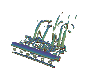
  $\lambda _2$ criterion in figure 5. Here,
  $\lambda _2$ is defined as the second-largest eigenvalue of the tensor
  $S_{ij}S_{ij}+\varOmega _{ij}\varOmega _{ij}$, where
  $S_{ij}$ and
  $\varOmega _{ij}$ are the symmetric and antisymmetric parts of the velocity gradient tensor, respectively (Jeong & Hussain Reference Jeong and Hussain1995). At higher
  $\beta =25\,\%$, it is observed that the spanwise vortex tubes undergo flow instabilities in the form of helical twisting and stretching (not evident at this time instant, but discussed in subsequent sections). Figure 5 is further striking and is indicating clearly that an already ‘turbulent’ state behind a non-perforated plate is tending towards relaminarization and is pushed further into a transitional state by the presence of perforation at the chosen
  $Re$. The instability modes will be discussed in further detail in § 3.6.

Figure 4. Instantaneous spanwise vorticity  $\omega _y=\pm (0.004\unicode{x2013}0.005)$: (a,c,e,g) side view depicting wake width; (b,d, f,h) bottom views, at (a,b)
  $\beta = 0\,\%$, (c,d)
  $\beta = 9\,\%$, (e, f)
  $\beta = 16\,\%$, and (g,h)
  $\beta = 25\,\%$.

Figure 5. Instantaneous  $\lambda _2$ from
  $-3\times 10^{-6}$ to
  $-4\times 10^{-6}$: (a)
  $\beta = 0\,\%$, (b)
  $\beta = 9\,\%$, (c)
  $\beta = 16\,\%$, (d)
  $\beta = 25\,\%$.
Next, the vortex characteristics of the first pair of counter-rotating vortex rollers shown in figures 4(a,c,e,g) are studied. At a given spanwise location, the circulation  $\varGamma _y$ and the vortex centre
  $X^c$ of a vortex with vorticity
  $\omega _y$ are calculated by
 $$\begin{gather} \varGamma _y= \int\int_D \omega _y \,{{\rm d}\kern0.06em x} \,{\rm d}z, \end{gather}$$
 $$\begin{gather}X^c= \frac{1}{\varGamma _y}\int\int_D X \omega _y \,{{\rm d}\kern0.06em x} \,{\rm d}z. \end{gather}$$
Here, the domain of integration  $D$ signifies the region enclosing the vortex, and
  $X$ is the coordinate of the surface element
  ${{\rm d}\kern0.06em x}\, {\rm d}z$ having vorticity
  $\omega _y$. The vortex separation distance
  $b$ between counter-rotating vortices is obtained from
 \begin{equation} b = |X_+^c -X_-^c|. \end{equation}
The subscripts ‘ $+$’ and ‘
 $-$’ denote the signs of the two counter-rotating vortices. The vortex separation is further decomposed into streamwise component
  $b_x$, and cross-stream component
  $b_z$.
These vortical quantities are averaged along the span and reported in table 4, where  $E_{peak}$ denotes the peak spectral energy associated with the
  $\hat {w}$ velocity signal, and
  $v_{rms}$ is used as a sufficient measure of three-dimensionality in the flow (Karniadakis & Triantafyllou Reference Karniadakis and Triantafyllou1992). It is observed that the variation of
  $E_{peak}$ with respect to
  $\beta$ follows a trend similar to
  $St_d$, where it increases up to
  $\beta =16\,\%$ followed by a sharp drop at
  $\beta =25\,\%$. In contrast,
  $b_z$ and
  $v_{rms}$ follow an inversely related trend. It can be deduced that as the three-dimensionality in the flow reduces, the counter-rotating vortices are brought closer to each other in the cross-stream direction
  $b_z$, causing increased spectral energy
  $E_{peak}$. This leads to a larger streamwise separation
  $b_x$, with a higher shedding frequency, or
  $St_d$.
3.2.1. Instantaneous fluctuation of kinetic energy
Figure 6 shows iso-contours of instantaneous fluctuation kinetic energy, defined as  $k=\widehat {u_i}\widehat {u_i}/2$. Here, the occurrence of high-intensity spots in the ‘near’ wake at
  $\beta >0\,\%$ corresponds to the length of the ‘bleed’ jet core. The spanwise coherence of
  $k$ in the ‘far’ wake signifies the location of shear layer roll-up. The distribution of fluctuation kinetic energy in the ‘near’ and ‘far’ wakes shows clearly that the primary source of fluctuation energy in the ‘near’ wake is the jets emanating from perforation holes (see figures 6b,d, f,h). These jets are separated by wakes from the solid portion of the plate, resulting in an anisotropic and inhomogeneous flow. Such a jet–wake interaction produces a significant amount of shear. It appears that the length of the primary vortex formation around the ‘bleed’ jet varies with
  $\beta$, similar to the trend followed by
  $St_d$. Here, it is observed to increase from
  $\beta =9\,\%$ to
  $\beta =16\,\%$, followed by a reduction at
  $\beta =25\,\%$. At
  $\beta =16\,\%$, the length of the ‘bleed’ jet core nearly coincides with the location of shear layer roll-up, indicating the jet–wake coupling close to equilibrium. On the other hand, the coherent or unsteady motion is responsible for the high-fluctuation kinetic energy in the ‘far’ wake. Additionally, it could be seen here that the turbulence in the ‘near’ as well as ‘far’ wake (also see
  $v_{rms}$ in table 4) is suppressed gradually as
  $\beta$ increases towards
  $16\,\%$ with a corresponding rapid ascent of
  $St_d$ (see table 4). Because of the changing nature of the small-scale flows through the holes, the turbulence re-emerges at the higher
  $\beta$ of
  $25\,\%$. This is accompanied with a fall in
  $St_d$ from its elevated values at
  $\beta =9\,\%$ and
  $16\,\%$.

Figure 6. Instantaneous fluctuation kinetic energy at mid  $z/d$ plane: (a,c,e,g) whole domain; (b,d, f,h) the ‘bleed’ jet region (‘near’ wake). Note that
  $x/d=5$ indicates the plate location. Observe that the colour bar ranges differ between panels.
Further, the local Reynolds numbers are shown in table 5. Here,  $Re_m$ is defined based on the margin
  $m$ between two adjacent holes (see figure 1b), and
  $Re_h$ is defined based on the width of the hole,
  $h$. The local Reynolds number of the jet,
  $Re_{jet}$, is defined as
  $Re_{jet}=\bar {u}_{jet,max} h/\nu$, where
  $\bar {u}_{jet}$ indicates the jet centreline velocity, and subscript
  $max$ signifies maximum value along the centreline. At lower porosities, flow retardation is expected to be high, with vortex street dominating over ‘bleed’ flow, leading to
  $Re_{jet}< Re_m$. At higher porosities, ‘bleed’ flow controls the vortex street due to increased momentum with
  $Re_{jet}>Re_m$. At
  $\beta =16\,\%$, the ‘bleed’ flow is just enough to prevent the shear layers from interacting in the ‘near’ wake with
  $Re_{jet}\approx Re_m$. Thus it could be argued that the peculiar behaviour of quasi-laminar flow with weak three-dimensionality at
  $\beta =16\,\%$ is related to the fact that
  $Re_{jet}\approx Re_m$. Here, the ‘bleed’ jet is marginally longer with least three-dimensionality, as seen by the relatively lower
  $k$ in the ‘near’ wake (see figures 6b,d, f,h). At slightly higher
  $\beta =25\,\%$,
  $k$ revives to a larger value, indicating transition of the laminar ‘bleed’ jet to an irregular state. This could be due to proximity interference effects of adjacent jets when
  $h\gtrsim m$.
Table 5. Various Reynolds numbers shown here are defined as  $Re_h=U_o h/\nu$,
  $Re_{m}=U_o m/\nu$ and
  $Re_{jet}=\bar {u}_{jet,max} h/\nu$. Here,
  $m$ is also equal to
  $2s$ (cf. figure 1b).

Although the variation of  $St_d$ with
  $\beta$ in the current DNS follows a trend very similar to high
  $Re$ cases of Castro (Reference Castro1971), it is quite possible that the wake and ‘bleed’ flow vortex dynamics might be different at much higher
  $Re$. Nevertheless, it was presumed by Castro (Reference Castro1971) that the flow through the holes themselves affects
  $\overline {C_d}$ and
  $St_d$. The observations in this section indicate clearly that the local Reynolds number in the ‘near’ wake plays a primary role in determining the overall three-dimensionality of the flow, and the ‘near’ wake affects the behaviour of large vortical structures in the ‘far’ wake.
3.3. Spatio-temporal analysis
Figure 7 shows the spatio-temporal plot of cross-stream velocity  $w/U_o$ for various
  $\beta$. Here, the horizontal axis corresponds to the normalized time
  $tU_o/d$, and the vertical axis is the spanwise extent of the plate,
  $y/d$. The data in figures 7(a,c,e,g) are recorded from the ‘near’ wake at
  $1d$ downstream of the plate, while the data in figures 7(b,d, f,h) stem from the ‘far’ wake at
  $15d$ downstream of the plate. The spanwise alternate bands in the ‘far’ wake signify a Kármán-like vortex street. It is evident that the coherence in the spanwise bands in the ‘far’ wake increases with
  $\beta$ up to 16 %. In contrast, the incoherence increases from
  $\beta =16\,\%$ to
  $25\,\%$. On the other hand, it is observed that the spanwise vortex structures in the ‘near’ wake transition to streamwise vortex structures with an increase in
  $\beta$. Here, the streamwise alternate bands signify shear layer undulations under the influence of ‘bleed’ flow. Note that the wavelength of these waves is approximately equal to the geometric pitch of the perforations. Such a flow state in the ‘near’ wake indicates vortex street suppression at higher
  $\beta$, causing delayed shear layer interaction leading to monotonic decrease in
  $\overline {C_d}$.

Figure 7. The  $w$ velocity time trace sampled in (a,c,e,g) the ‘near’ wake (
 $1d$ downstream along the top edge of the plate,
  $z/d=8.5$), and (b,d, f,h) the ‘far’ wake (
 $15d$ downstream along the top edge of the plate,
  $z/d=8.5$).
Figures 8 and 9 show the corresponding time trace of the spanwise and cross-stream velocity signals in the ‘near’ and ‘far’ wakes, respectively. Figure 8 further supports the vortex street suppression at higher  $\beta$, demonstrated by reduced irregularities in the
  $v$ and
  $w$ velocity signatures. The signals at
  $\beta =16\,\%$ are nearly quiescent, indicating vortex street suppression leading to undulating shear layers in the ‘near’ wake. Here, the quiescent flow also suggests quasi-laminar characteristics. It has already been observed by fluctuation kinetic energy, and it will also be shown later by ‘bleed’ flow characteristics and secondary instabilities, that a weak three-dimensionality exists at
  $\beta =16\,\%$. The revival of three-dimensionality at
  $\beta =25\,\%$ could be due to local
  $Re$ effects where the neighbouring ‘bleed’ jets interact with each other when
  $h\gtrsim m$. Further, the ‘bleed’ jets undergo meandering instability due to proximity interference effects (discussed further in § 3.7). On the other hand, figure 9 demonstrates the vortex street behaviour in the ‘far’ wake. The
  $w$ velocity signal at
  $\beta =0\,\%$, coupled with higher fluctuations in the
  $v$ velocity, indicates the irregular behaviour of the vortex street. With increasing
  $\beta$, the irregularities reduce, leading to a quasi-periodic state with weak three-dimensionality at
  $\beta =16\,\%$. At
  $\beta =25\,\%$, the
  $v$ velocity fluctuations increase, indicating revival of three-dimensionality in the flow. Overall, it is clear that the low-
 $Re$ turbulent state at
  $\beta =0\,\%$ is pushed back to a transitional state by the perforations. A similar phenomenon is also reported in the wakes of circular cylinders, where addition of dilute concentrations of polymer additives causes turbulence suppression (Richter, Iaccarino & Shaqfeh Reference Richter, Iaccarino and Shaqfeh2010, Reference Richter, Iaccarino and Shaqfeh2012).

Figure 8. Velocity time trace sampled in the ‘near’ wake ( $1d$ downstream of the plate along the top edge of the plate,
  $y/d=0$,
  $z/d=8.5$): (a,c,e,g)
  $v/U_o$, (b,d, f,h)
  $w/U_o$.

Figure 9. Velocity time trace sampled in the ‘far’ wake ( $15d$ downstream of the plate along the top edge of the plate,
  $y/d=0$,
  $z/d=8.5$): (a,c,e,g)
  $v/U_o$, (b,d, f,h)
  $w/U_o$.
3.4. Spectral analysis
Fast Fourier transforms of the instantaneous  $\hat {w}$ velocity signal sampled over 60 vortex shedding cycles are shown in figure 10. Figures 10(a,c,e) show the Fourier spectrum of the signal in the ‘near’ wake, whereas figures 10(b,d, f) show that of the ‘far’ wake. Here,
  $f_s$ denotes the Strouhal number corresponding to the dominant frequency. Figures 10(a,b) show that the dominant
  $St_d$ is the same in both the ‘near’ and ‘far’ wakes for
  $\beta =9\,\%$, signifying that the effect of the ‘bleed’ jet is not strong enough to push the formation of a vortex street downstream by a significant margin. In the
  $\beta =16\,\%$ case, distinct dominant frequencies emerge. Figures 10(c,d) show that in the ‘near’ wake spectrum, the most dominant frequency corresponds to
  $St_d = O[10^{-3}]$, which is insignificant. The next distinct value,
  $St_d = 0.185$, interestingly becomes the most dominant one in the ‘far’ wake. Note that a single dominant frequency was reported in Castro (Reference Castro1971), where the origin of the signal recording position is not particularly clear. (Note that Castro (Reference Castro1971) used circular holes and the experiments were conducted at higher
  $Re$.) In addition, figures 10(c,d) also show the presence of distinct higher harmonics of the Strouhal frequency containing a specific periodicity, further supporting the quasi-laminar behaviour described in the previous subsections.

Figure 10. Fast Fourier transforms of the  $\hat {w}$ velocity sampled at (a,c,e) the ‘near’ wake (
 $1d$ downstream along the top edge of the plate,
  $y/d=0$,
  $z/d=8.5$), and (b,d, f) the ‘far’ wake (
 $15d$ downstream along the top edge of the plate,
  $y/d=0$,
  $z/d=8.5$), for (a,b)
  $\beta = 9\,\%$, (c,d)
  $\beta = 16\,\%$, (e, f)
  $\beta = 25\,\%$. Here,
  $f_s$ denotes the dominant
  $St_d$.
3.5. Two-point correlation
Figure 11 shows the spanwise two-point correlation of all the velocity components in the ‘near’ and ‘far’ wakes. Here, the correlation coefficient is defined as  $\rho _{\phi \phi }= \overline {\hat {\phi } (x,y,z,t)\,\hat {\phi } (x,y+\delta y,z,t)}/\overline {\hat {\phi } (x,y,z,t)^2}$, where
  $\hat {\phi }\in (\hat {u},\hat {v},\hat {w})$. The overline signifies time averaging over 75 vortex-shedding cycles. In the ‘near’ wake, the streamwise and cross-stream velocity components remain highly correlated at lower
  $\beta$ (see
  $\rho _{uu}$ and
  $\rho _{ww}$, respectively, in figures 11a,e) due to the formation of a spanwise-coherent Kármán vortex street (see figure 4). The correlation is lower at higher
  $\beta$ as the dominant ‘bleed’ flow suppresses the vortex shedding. Here, the oscillatory nature of correlation for perforation cases, i.e. at
  $\beta >0\,\%$, is due to the effect of periodically spaced ‘bleed’ flow through holes. For similar reasons, the uncorrelated nature of the spanwise velocity component at
  $\beta =0\,\%$ deviates marginally with increasing
  $\beta$ (see
  $\rho _{vv}$ in figure 11c). The irregular behaviour of the correlation functions along the span could be due to the limited number of samples considered for averaging (Singh & Narasimhamurthy Reference Singh and Narasimhamurthy2021). In the ‘far’ wake, the streamwise and cross-stream correlations remain correlated in all cases (see figures 11b, f) due to the presence of spanwise vortex tubes (see figure 4). Interestingly,
  $\rho _{uu}$ and
  $\rho _{ww}$ follow a trend similar to that of
  $St_d$, where the correlation increases with
  $\beta$ at 0 % to 16 %, followed by a slight drop at 25 %. Also,
  $\rho _{vv}$ shows a similar trend with negative correlation (see figure 11d). Thus it can be noted that all the velocity components show high correlation at
  $\beta =16\,\%$ due to ‘quasi-periodic’ vortex tubes in the ‘far’ wake (see figure 4).

Figure 11. Two-point correlation  $\rho$ at (a,c,e) the ‘near’ wake (
 $1d$ downstream along the top edge of the plate,
  $z/d=8.5$), and (b,d, f) the ‘far’ wake (
 $15d$ downstream along the top edge of the plate,
  $z/d=8.5$), for (a,b)
  $\widehat {uu}$, (c,d)
  $\widehat {vv}$, (e, f)
  $\widehat {ww}$.
3.6. Modes of instability
Figure 12 shows the iso-contours of streamwise vorticity at all  $\beta$ considered in the present study. The instability mode for the non-perforated plate is reported to have mode B vortex structure by Najjar & Balachandar (Reference Najjar and Balachandar1998), where reasonably well organized streamwise vortices with spanwise wavelength
  ${\approx }1.2$ are observed to extend in the braid region connecting the Kármán vortices. The strain field induced by the streamwise vorticity significantly distorts the spanwise Kármán vortices. Nevertheless, the spanwise and streamwise vortices are observed to be distinct (see figure 5). Although the vortex structure is observed to be slightly chaotic at lower porosities in the present study, the symmetry pattern at the higher porosity of
  $\beta =16\,\%$ appears similar to a mode B structure observed by Williamson (Reference Williamson1996b) for circular cylinder wakes, where mode B is defined as a secondary vortex structure with symmetric pattern of streamwise vortices from one braid region to the next. Figure 12 further indicates the effect of perforation on the secondary instabilities. Here, the vortical structures with spanwise wavelength
  ${\approx }1d$ in the ‘near’ wake of perforation cases correspond to the vorticity arising due to the effect of ‘bleed’ flow. In the ‘far’ wake, it appears that the prevailing secondary instability tends towards coherence and spatial compactness as
  $\beta$ is increased up to 16 %. The spanwise wavelength of this transition mode in the present perforated case is
  ${\approx }1d$ (i.e. six pairs along the span), in contrast to
  ${\approx }2d$ of the short-wavelength mode reported for non-perforated plates (Julien et al. Reference Julien, Lasheras and Chomaz2003, Reference Julien, Ortiz and Chomaz2004; Thompson et al. Reference Thompson, Hourigan, Ryan and Sheard2006) and
  ${\approx }1d$ of mode B reported for circular cylinders (Williamson Reference Williamson1996a). The spanwise coherence is also seen to increase for Kármán vortex structures. At
  $\beta = 16\,\%$, the wake instability (cf. figures 5c and 12c) appears to behave as quasi-laminar since the wake experiences periodic oscillations (cf. figure 9(b,d, f,h)). However, there exists the presence of fine-scale streamwise vortex structures. This case resembles closely the resonance state of the wake behind circular cylinders (Williamson Reference Williamson1996b). Further, figure 12(d) indicates that the prevailing secondary instability in the ‘far’ wake at
  $\beta = 25\,\%$ is signified by an antisymmetric pattern of streamwise vortices having spanwise wavelength
  ${\approx }2d$. This flow state has some resemblance to the mode A instability in the wake of circular cylinders.

Figure 12. Three-dimensional iso-contours of streamwise vorticity  $\omega _x =\pm (0.002\unicode{x2013}0.003)$, for (a)
  $\beta = 0\,\%$, (b)
  $\beta = 9\,\%$, (c)
  $\beta = 16\,\%$, (d)
  $\beta = 25\,\%$. Yellow and black colours indicate positive and negative values of
  $\omega _x$, respectively.
3.7. Bleed flow (jet) oscillation
In this study, we also observed another interesting phenomenon, where the jet or ‘bleed’ flow is experiencing an oscillatory motion along the spanwise direction (i.e. in the  $x\unicode{x2013}y$ plane). This meandering jet instability is captured in the instantaneous rotation rate field, defined by
  $\varOmega _z=\partial u/\partial y-\partial v/\partial x$ (cf. figure 13). It appears that the meandering instability is profound as
  $\beta$ is increased to 25 %. It has been reported in the literature that if the pitch
  $c/h$ or the gap is sufficiently small, then the adjacent shear layers in a wake can experience proximity interference effects leading to engulfment or meandering oscillations and instabilities (Dadmarzi et al. Reference Dadmarzi, Narasimhamurthy, Andersson and Pettersen2018). The time trace of spanwise and cross-stream velocities sampled in the ‘near’ wake at the jet-central location (cf. figure 14) further substantiates this instability. Here, it is observed that the ‘bleed’ flow at
  $\beta = 9\,\%$ experiences low-frequency oscillations in the spanwise direction. In addition, it undergoes high-frequency oscillations in the cross-stream direction, indicating a strong influence of the vortex street. At
  $\beta =16\,\%$, the ‘bleed’ flow undergoes high-frequency oscillations in both the spanwise and cross-stream directions. The low amplitude of
  $v$ and
  $w$ velocity signals are in line with reduced three-dimensionality and vortex shedding suppression, respectively. At
  $\beta = 25\,\%$, high-frequency high-amplitude jet meandering is evident from the oscillatory high-frequency
  $v$ velocity signal. At the same time, a low-amplitude
  $w$ velocity signal signifies the absence of Kármán vortex shedding. The frequency of meandering is further quantified by the fast Fourier transform of the
  $\hat {v}$ velocity signal (cf. figure 15). The corresponding
  $St_d$ at
  $\beta =9\,\%$ is found to be negligibly small. On the other hand, the dominant meandering frequency is significantly higher at
  $\beta \geqslant 16\,\%$ with
  $St_d=0.187$.

Figure 13. Instantaneous rotation rate at the wake centreline ( $z/d=8$) showing the flapping mechanism of the ‘bleed’ flow through the holes (jet).

Figure 14. Velocity time trace sampled at  $y/d=2.5$,
  $z/d=8$ (i.e. along the centreline of the third hole), for (a,c,e)
  $v/U_o$, (b,d, f)
  $w/U_o$. Sampling across the streamwise direction is done at
  $1d$ downstream of the plate for
  $\beta = 9\,\%$ or
  $2d$ downstream of the plate for
  $\beta \geqslant 16\,\%$ due to differential jet length.

Figure 15. (a,c,e) Fast Fourier transforms of the  $\hat {v}$ velocity sampled at
  $y/d=2.5$,
  $z/d=8$ (i.e. along the centreline of the third hole), and (b,d, f) spectra along the span, at (a,b)
  $\beta =9\,\%$, (c,d)
  $\beta =16\,\%$, (e, f)
  $\beta =25\,\%$. Sampling along the streamwise direction is done at
  $1d$ downstream of the plate for
  $\beta = 9\,\%$ or
  $2d$ downstream of the plate for
  $\beta \geqslant 16\,\%$ due to differential jet length.
3.8. Mean primary and secondary flow
Figure 16 shows the mean streamwise velocity along the plate centreline, i.e. through the solid section of the plate, as well as along the hole centreline. The region along the  $x$ axis with negative velocity signifies the presence of a recirculation zone. From figure 16(a), it is observed that the primary recirculation zone, i.e. the recirculation along the plate centreline, is present predominantly at all
  $\beta$. However, the secondary recirculation, i.e. recirculation along the hole centreline shown in figure 16(b), diminishes in size and eventually disappears at
  $\beta =25\,\%$. This is due to the fact that the ‘bleed’ flow pushes the vortex downstream with increasing
  $\beta$. Furthermore, the peak streamwise velocity with
  $\bar {u}/U_o>1$ shows the jet-like effect of the ‘bleed’ flow. It appears that the peak jet velocity reduces while its location is shifted downstream with increase in
  $\beta$ from 9 % to 25 % (also quantified earlier as
  $\bar {u}/{U_o}_{jet,max}$ in table 4).

Figure 16. Mean primary flow along (a) the plate centreline, and (b) the hole centreline (averaged in time and along the pitch).
Additionally, a strong mean secondary flow (i.e. the spanwise velocity  $\bar {v}/U_o$) is observed both upstream and downstream of the perforated plates. Figures 17(a,c) show contours of mean secondary flow upstream and downstream of the plate, respectively, at
  $\beta =9\,\%$. The corresponding mean pressure contours are shown in figures 17(b,d). Note that the data are averaged in time and along the pitch. It appears that the maximum secondary flow upstream of the plate occurs at
  $y/d\approx 0.35$ and
  $0.65$. This location corresponds to the edge of the square hole. The corresponding pressure contours show a high-pressure region away from the hole, indicating that the flow is driven by differential pressure towards the hole along the path of least resistance. In comparison, the maximum secondary flow downstream of the perforated plates is observed to be
  ${\approx }15\,\%$ of the inflow velocity. Similar observations can be made at higher
  $\beta$ (not shown here). Further, figure 18 shows the variation of mean secondary flow along the streamwise direction at various spanwise locations. It is clear from figure 18(b) that the mean secondary flow downstream of the perforated plates is significantly higher in the formation region. In contrast, the mean secondary flow is negligibly small for the non-perforated plate. In the ‘far’ wake, it reduces to a negligible value for both the perforated and non-perforated cases.

Figure 17. Secondary flow (averaged in time and along the pitch) at  $z/d=8$ (i.e. mid
  $z$ plane) for
  $\beta =9\,\%$: (a)
  $\bar {v}/U_o$ upstream of the plate; (b)
  $\bar {p}/(\rho U_o^2)$ upstream of the plate; (c)
  $\bar {v}/U_o$ downstream of the plate; (d)
  $\bar {p}/(\rho U_o^2)$ downstream of the plate.

Figure 18. Secondary flow averaged in time and along the pitch,  $\bar {v}/U_o$, at
  $z/d=8$ (i.e. mid
  $z$ plane): (a) upstream of the plate; and (b) downstream of the plate.
4. Conclusion
In the present DNS study, the effect of perforation on the wake of a low- $Re$ turbulent flow over a flat plate placed normal to the free stream is studied. It is observed that the current mean drag coefficient
  $\overline {C_d}$, and the Strouhal number
  $St_d$, have excellent qualitative agreement with the high-
 $Re$ experiments of Castro (Reference Castro1971), i.e. despite the differences in
  $Re_d$ and perforation shape pattern. Further, the vortex street is pushed farther downstream by the bleed (jet) flow through the perforations, leading to monotonically decreasing
  $\overline {C_d}$ with respect to
  $\beta$. As
  $\beta$ is increased, the spanwise vortex tubes in the near wake cease to exist, paving their way to streamwise vortex filaments signifying the bleed flow. Under its influence, the shear layers undergo undulations in the near wake, while their interaction is pushed farther downstream with the emergence of a vortex street in the far wake. The vortex street suppression leads to a sharp fall in
  $\overline {C_d}$, with its apparent reduction observed to begin at
  $\beta \approx 4\,\%$. Castro (Reference Castro1971) observed this phenomenon at
  $\beta \approx 20\,\%$. Such a dissimilarity may be a consequence of the vast difference in
  $Re$ in both studies. In contrast, the increase in
  $St_d$ with respect to
  $\beta$ followed by a sudden drop at
  $\beta \approx 20\,\%$ is predicted in both studies. In the present study, a distinct dominant frequency exists at
  $\beta \geqslant 16\,\%$ in the near wake and far wake, corresponding to the shear layer undulations and the vortex street, respectively. This is in contrast to a single dominant frequency reported by Castro (Reference Castro1971), where the origin of the signal recording position is not particularly clear. Additionally, a higher magnitude of
  $St_d$ is observed here when compared to that reported by Castro (Reference Castro1971). This can be attributed to the lower
  $Re_d$ in the current DNS. Castro (Reference Castro1971) suggests two distinct flow regimes appropriate to low and high porosities, with a sudden transition between the two regimes at this point as a consequence of a vortex street suddenly ceasing to exist. Here, it was presumed that the bleed flow is just enough to prevent shear layer interaction completely. Also, the dominant frequency was believed to be due to some kind of far wake instability, where the two shear layers are assumed to coalesce downstream, leading to a flapping wake. On the other hand, Huang et al. (Reference Huang, Ferré, Kawall and Keffer1995) and Huang & Keffer (Reference Huang and Keffer1996) propose that the small-scale vortices in the formation region merge to form quasi-periodic Kármán-like structures in the far wake at high porosities. In contrast, the shear layers are observed to interact farther downstream to form a vortex street at least up to
  $\beta =25\,\%$ in the present study. Note that such a dissimilarity may be a direct consequence of the
  $Re$ effect and limited porosity cases considered here.
In the current study, a low- $Re$ turbulent wake from a non-perforated plate is altered to a transitional state by the presence of perforation. The flow gradually relaminarizes , i.e. suppresses turbulence, as
  $\beta$ is increased from 0 % to 16 %. The strong bleed flow at
  $\beta =16\,\%$ renders the wake ‘quasi-laminar’ with weak flow three-dimensionality. This explains the increase in
  $St_d$ when
  $\beta$ is increased from 0 % to 16 %. Note that the near wake characterized by the jet or bleed flow also undergoes a similar reduction in flow three-dimensionality. At a higher
  $\beta$ of 25 %, the spanwise vortex tubes undergo helical twisting and stretching with a drop in
  $St_d$. Such a behaviour is coupled with the revival of three-dimensionality in the near wake due to the proximity interference effects of adjacent jets. The enhanced proximity effects (when pitch separation is equivalent to the hole size) also cause the jets to be meandering at
  $St_d=0.187$. Thus it is clear that the local Reynolds number
  $Re_h$ (defined based on the hole size) in the near wake determines the overall three-dimensionality of the flow, and the near wake influences the behaviour of large vortical structures in the far wake. Nevertheless, it is quite possible that the wake and bleed flow vortex dynamics is different at much higher
  $Re$. In particular, the near wake may also be a function of the geometry (e.g. shape and size) of the perforations. It may be expected that a smaller hole size at a given
  $\beta$ may increase flow retardation, while a larger hole size may increase bleed jet coalescence or meandering.
As a result of turbulence suppression, the streamwise vortex pairs of secondary instabilities become fairly regular and organized as  $\beta$ is increased from 0 % to 16 %. The ‘quasi-laminar’ state at
  $\beta =16\,\%$ is coupled with the existence of fine-scale streamwise vortices structured in an orderly manner. The prevailing secondary instability at this porosity value appears similar to a mode B structure, with a symmetric pattern of streamwise vortices from one braid region to the next, with spanwise wavelength
  ${\approx }1d$. However, at higher porosity
  $\beta =25\,\%$, the secondary instability is signified by an antisymmetric pattern of streamwise vortices, with spanwise wavelength
  ${\approx }2d$. Note that such an instability is observed to occur intermittently in space and time, resembling mode A instability reported by Williamson (Reference Williamson1996a).
Funding
This work has received support from the Centre for Industrial Consultancy and Sponsored Research, IIT Madras and the P.G. Senapathy Center for Computing Resource through a grant of computing time. The authors also thank P. Jadhav and D.I. Poojary, Department of Applied Mechanics, Indian Institute of Technology Madras, for facilitating additional DNS jobs on the cluster.
Declaration of interests
The authors report no conflict of interest.
Appendix A. Grid verification
Two-dimensional simulations of flow over a normal flat plate and two side-by-side plates are considered first as limiting cases of the present perforated plate. The resulting mesh  $[N_x,N_z]$ from the grid test (see figure 19) is then used for the 3-D grid study (perforated plate of
  $\beta =25\,\%$), where equidistant grid size (
 $\varDelta _y$) is varied along the span. Table 6 summarizes the results. Here, the Strouhal number and mean drag coefficient, defined as
  $St_d=f d/U_o$ and
  $\overline {C_d}=({\bar {p}_{front}-\bar {p}_{back}})/({0.5 \rho U_o^2})$, respectively, are used as the criteria for a grid independence study, where
  $f$ is the dominant wake frequency, and
  $\rho$ is the fluid density. Here,
  $\bar {p}_{front}$ and
  $\bar {p}_{back}$ denote the mean pressures on the front and back surfaces of the plate, respectively.

Figure 19. Mesh topology in an  $x\unicode{x2013}z$ plane.
Table 6. Mesh convergence test. The Strouhal number  $St_d$ is recorded at
  $15d$ downstream of the plate. Here,
  $h$ refers to the hole or gap size between the plates. See Singh & Narasimhamurthy (Reference Singh and Narasimhamurthy2021) for more details.

Appendix B. Spanwise domain verification
The effect of spanwise extent of the domain on the Strouhal number, drag coefficient and wake dynamics is assessed by varying the spanwise length of the plate. Here, the aspect ratio  $AR$, defined as the ratio of domain span to width of the plate, is varied between 1, 3, 6 and 12. It is observed from table 7 that the integral quantities
  $St_d$ and
  $\overline {C_d}$ do not vary much with
  $AR$. This could be explained by the vortex street formation region, where the primary recirculation zone is pushed downstream by the bleed flow, irrespective of
  $AR$. On the other hand, the wake dynamics is starkly different at
  $AR\leqslant 3$ and
  $AR\geqslant 6$, as shown by the instantaneous vortex topology of
  $\lambda _2$ contours in figure 20. The wake at
  $AR\leqslant 3$ is fairly coherent with spanwise vortex cores parallel to the plate span. At
  $AR\geqslant 6$, the wake experiences incoherence of the spanwise vortex cores (see Singh & Narasimhamurthy (Reference Singh and Narasimhamurthy2021) for more details). From a computational cost perspective,
  $AR=6$ is therefore chosen for further studies.
Table 7. The Strouhal number  $St_d$ and mean drag coefficient
  $\overline {C_d}$ for various aspect ratios
  $AR$ of a perforated plate at
  $\beta =25\,\%$. Here,
  $St_d$ is recorded in the far wake at
  $15d$ downstream along the top edge of the plate,
  $z/d=8.5$.


Figure 20. Instantaneous  $\lambda _2$ contours depicting vortex topology for various
  $AR$ of perforated plate at
  $\beta =25\,\%$.
Appendix C. Influence of domain blockage
The blockage effect has been examined for a perforated plate of porosity  $\beta =25\,\%$. Here, two domains of blockage ratios 6.25 % and 3.125 % are considered (see table 8 for details). The blockage
  $B$ is defined by
  $d/L_z$. The mesh size in the large domain,
  $[N_x, N_y, N_z] = [360, 240, 420]$, is such that the grid quality remains the same. It is observed that the drag coefficient varies by about 7.2 % between the cases. Such a variation is expected in bluff-body flows in (finite domain) numerical studies and closed wind tunnel experiments (also seen in the experiments of Fage & Johansen (Reference Fage and Johansen1927) and reported by Maskell (Reference Maskell1965)). Maskell (Reference Maskell1965) proposed the following equation for blockage correction, where
  $\overline {{C_d}_c}$ is the corrected drag coefficient, and
  $\epsilon$ is the blockage constant equal to 0.96:
 \begin{equation} \frac{\overline{C_d}}{\overline{{C_d}_c}} = 1 + \epsilon \overline{C_d} B. \end{equation}
It can also be noted from table 8 that the corrected drag coefficient from the present domain is close to the computed drag coefficient from the larger domain. Furthermore, the 3-D  $\lambda _2$ contours are depicted in figure 21 for domains with blockage ratios 6.25 % and 3.125 %, respectively. (The plate is located at
  $x/d=5$ for the present domain, and
  $x/d=11$ for the larger domain.) Here, similarities are observed in both cases, such as the near wake structures, emergence of spanwise structures at
  ${\approx }5d$ downstream of the plate, emergence of a vortex street at
  ${\approx }12d$ downstream of the body, and existence of streamwise structures originating from the vortex tube located close to the outlet. The streamwise vorticity contours shown in figure 22 depict similar behaviour in both the cases. Considering the computational cost, the present domain is chosen for further parametric studies.

Figure 21. Instantaneous  $\lambda _2$ from
  $-3\times 10^{-6}$ to
  $-4\times 10^{-6}$ depicting the vortex topology of a perforated plate at
  $\beta =25\,\%$: (a) domain
  $L_x \times L_y \times L_z = 25 \times 6 \times 16$; (b) domain
  $L_x \times L_y \times L_z = 31 \times 6 \times 32$.

Figure 22. Instantaneous 3-D iso-contours of streamwise vorticity  $\omega _x=\pm (0.002\unicode{x2013}0.003)$ of a perforated plate at
  $\beta =25\,\%$. Yellow and black colours indicate positive and negative values of
  $\omega _x$, respectively: (a) domain
  $L_x \times L_y \times L_z = 25 \times 6 \times 16$; (b) domain
  $L_x \times L_y \times L_z = 31 \times 6 \times 32$.
Table 8. Influence of domain blockage on  $\overline {C_d}$ and
  $St_d$ for a perforated plate at
  $\beta =25\,\%$. Here, the domain length is varied in the streamwise (upstream of the plate) and cross-stream directions. The blockage ratio is defined as
  $(d/L_z)\times 100$.


 Open access