


1. Introduction
Gravity flow of elongated drops in circular vertical pipes is frequent in both industrial processes and natural systems. The early contribution by Beirute & Flumerfelt (Reference Beirute and Flumerfelt1977) analysed the laminar displacement of drilling muds in a pipe due to the pumping of cement slurry, modelling both fluids as non-Newtonian with yield stress. The analytical approach focused on the most favourable conditions for effective mud displacement during cementing, and a detailed analysis of the role of several important variables was performed in achieving the objective. Subsequent analyses were devoted to the buoyancy driven exchange flows of two Bingham fluids in a cylindrical inclined duct, where viscoplastic and buoyancy forces almost balance one another (Frigaard & Scherzer Reference Frigaard and Scherzer1998, Reference Frigaard and Scherzer2000; Bittleston, Ferguson & Frigaard Reference Bittleston, Ferguson and Frigaard2002; Pelipenko & Frigaard Reference Pelipenko and Frigaard2004a), in most cases in the presence of an annulus gap unwrapped in a Hele-Shaw cell of varying gap. It is noteworthy that Frigaard & Scherzer (Reference Frigaard and Scherzer1998) presented, alongside a discussion of an engineering problem, a detailed analysis of the deviatoric stress in the unyielded region. In this same flow field geometry, interface instabilities and travelling wave solutions were also analysed; see Pelipenko & Frigaard (Reference Pelipenko and Frigaard2004b), who derived the stability/instability conditions of the front during displacement on the basis of rigorous Navier–Stokes equations and well-defined scaling arguments. In addition to the theoretical studies, numerous experiments have been carried out to measure the distribution of velocity and concentration in gravity currents of Newtonian fluids flowing in inclined tubes (see e.g. Seon et al. Reference Seon, Hulin, Salin, Perrin and Hinch2006).
In natural systems, gravity flow of elongated drops in circular vertical pipes mimics magma flows in volcanoes, where degassing and temperature effects induce vertical exchange between fluids of different density and viscosity (Kazahaya, Shinohara & Saito Reference Kazahaya, Shinohara and Saito1994; Stevenson & Blake Reference Stevenson and Blake1998; Llewellin & Manga Reference Llewellin and Manga2005). Other than magma ascension during eruptions, the phenomenon is typically associated with lock-exchange flows, and is controlled by the density difference between the ascending and the descending fluids, and by their viscosity. We note that we mean fluid ascending on average, since, depending on the characteristics of the flow field, part of the lighter fluid may be dragged downwards by the denser fluid, producing a backflow. In a typical configuration, gas Taylor bubbles (Taylor Reference Taylor1961), symmetric and bullet shaped, ascend near the axis of the pipe, while the heavier fluid descends, remaining in contact with the walls. This well-defined process has received attention from numerous researchers, who developed analytical models and performed experimental measurements, in particular for elongated gas bubbles in circular pipes (Viana et al. Reference Viana, Pardo, Yánez, Trallero and Joseph2003). In terms of dominant forces, the balance can be between buoyancy and (i) inertia, (ii) viscosity or (iii) surface tension. The ascent speed scales with different variables and parameters, and the flow stability is affected by the numerical value of relevant dimensionless parameters. In the buoyancy–inertia regime, the ascent speed is proportional to  $\sqrt {gR}$, where g is gravity and
  $R$ is the radius of curvature in the region of the vertex (Davies & Taylor Reference Davies and Taylor1950). In the buoyancy–viscosity regime, the ascent speed is
  ${\propto }{\rm \Delta} \rho gD^2/\mu$ where
  $\rho$ and
  $\mu$ are the fluid density and dynamic viscosity and
  $D$ is the equivalent diameter of the bubble. In some cases, inertial, capillary and viscous forces are of the same order of magnitude, and the ascent speed expression varies according to the flow regime (see Peebles Reference Peebles1953; Wallis Reference Wallis1969).
A key element in the rise of Taylor bubbles in vertical circular pipes is the thickness of the descending liquid film, experimentally analysed by Llewellin et al. (Reference Llewellin, Del Bello, Taddeucci, Scarlato and Lane2012) for Newtonian fluids as a function of a buoyancy Reynolds number  $D\sqrt {gD}/\nu$, where
  $D$ is the pipe diameter and
  $\nu$ is the fluid kinematic viscosity. A reduction in film thickness causes an increase in the skin friction drag on the bubble, with a rate depending on
  $\nu$ in the viscous regime; conversely, buoyancy also increases. As a result, the film thickness is inversely proportional to the buoyancy Reynolds number. If surface tension is considered, the film thickness also undergoes a decrease with increasing Eötvös number, defined as the ratio of gravitational to capillary forces, even to the point of blocking bubble rise when surface tension is dominant.
Similar analyses have been conducted for bubbles rising in the presence of non-Newtonian fluids (Shosho & Ryan Reference Shosho and Ryan2001). However, the results appear to be unconvincing also because the fluid rheology is largely disregarded; some indications may be inferred from the nature of the non-Newtonian fluid (e.g. carboxymethyl cellulose mixtures are generally shear thinning), but the characterization is poor and, in defining dimensionless groups, reference is generically made to the average viscosity measured at low shear-rate values. No significant influence on the bubble rise is attributed by Shosho & Ryan (Reference Shosho and Ryan2001) to the fluid rheology.
There exist a number of recent studies on bubbles displaced by flows of non-Newtonian ambient fluids in different contexts. Jalaal & Balmforth (Reference Jalaal and Balmforth2016) conducted a lubrication analysis of the thin films buffering a long bubble that is displaced down a slit or tube by ambient viscoplastic fluid flow. Laborie et al. (Reference Laborie, Rouyer, Angelescu and Lorenceau2017) revisited the classical Taylor and Bretherton film deposition problem in a circular channel adopting a yield-stress shear-thinning fluid rather than a Newtonian one. Zare, Daneshi & Frigaard (Reference Zare, Daneshi and Frigaard2021) observed experimentally and studied theoretically that bubbles rising in a yield-stress fluid create pathways that are preferentially followed by subsequent bubbles. Shemilt et al. (Reference Shemilt, Horsley, Jensen, Thompson and Whitfield2022) performed a stability analysis of an axisymmetric layer of a viscoplastic Bingham liquid coating the interior of a rigid tube, modelling an airway in the presence of mucus.
A behaviour akin to Taylor bubbles is observed in Taylor drops, which consist of a liquid rather than a gas. In this case, the dynamics of the ascending liquid becomes as important as that of the descending liquid, and requires further investigation in order to evaluate, for example, the speed of ascent or the thickness of the descending liquid film. Taylor drops form naturally, e.g. in volcanic chimneys as a result of degassing, which generates a magma of lower density than the ambient liquid and substantially affects viscosity (Francis, Oppenheimer & Stevenson Reference Francis, Oppenheimer and Stevenson1993) by causing crystallization of a mass fraction. In this regard, the conveyor-belt scheme proposed by Huppert & Hallworth (Reference Huppert and Hallworth2007) is of particular interest: the magma, relatively rich in gas (sulphur dioxide is mainly considered, due to the easy measurements with respect to other gases) rises in the volcanic chimney and, once at the surface, releases the gas into the atmosphere. Near the surface, the process is amplified by the pressure drop, as the gas bubbles increase their size and more bubbles develop according to Henry's law. Gas liberation, with the growth of crystals, in turn produces an increase in the average density of magma, and the process is also accentuated by cooling that results in a viscosity increase: thus denser and more viscous magma is available, which sinks into the chimney with a movement of a convective nature that leads to a much lower average erupted flow rate than is actually recirculated. This is why the evaluation of the magma flow rate based on the measured amount of sulphur dioxide overestimates the actual flow rate by several orders of magnitude.
In describing the convective motion of magma, we have assumed so far that the less dense magma rises near the conduit axis, while the denser magma descends at its periphery. Actually, this configuration is only one among the several possible forms of the process, since numerous experimental tests have shown different flow regimes as a function of the viscosity ratio (also defined viscosity contrast) between the descending and ascending fluids,  $\mathcal {M}=\mu _d/\mu _a$: according to Kazahaya et al. (Reference Kazahaya, Shinohara and Saito1994), the ascending fluid is near the axis only if
  $\mathcal {M}>300$; it occupies the periphery of the conduit, remaining adherent to the walls, for
  $\mathcal {M}<10$; for
  $10<\mathcal {M}<300$ the descending fluid splits into blobs. In fact, the classification of the field geometry appears vague, since the counter-flux of two fluids in vertical pipes is largely unstable (Joseph et al. Reference Joseph, Bai, Chen and Renardy1997). Indeed, several authors have been interested in the stability of core-annular flow in the various possible configurations, performing linear (Hickox Reference Hickox1971) or nonlinear (Chen & Joseph Reference Chen and Joseph1991) analyses. A common conclusion is that for a high viscosity contrast and due to the effect of surface tension, a core-annular flow that is inherently unstable appears stable or possibly metastable, with the presence of standing waves (bamboo and corkscrew) (see e.g. Bai, Chen & Joseph Reference Bai, Chen and Joseph1992). Stability has been analysed in depth by Suckale et al. (Reference Suckale, Qin, Picchi, Keller and Battiato2018): they conclude that bistability is inherent to core-annular flows, and it is not possible to predict which of the two possible equilibrium configurations (thin- and thick-core solutions) actually takes place on the basis of pipe geometry and fluid rheology alone. Instead, it is necessary to consider the boundary conditions.
In general, we expect the mechanics of Taylor drops and of slug flows or elongated drops generated by a lock exchange to be different, but as long as the viscosity difference between the two fluids is at least one order of magnitude, the speed of rise is the same (Stevenson & Blake Reference Stevenson and Blake1998). This enables collapse of the results of experiments despite the differences in the geometry of the flow field.
The buoyancy-driven flow of Taylor drops in the buoyancy–viscous regime has been analysed in detail by Picchi, Suckale & Battiato (Reference Picchi, Suckale and Battiato2020), using mechanical energy budgets including dissipation to correctly scale the radius and the speed of rise of the drops. In the non-dissipative regime, the dimensionless radius of the drops during steady-state ascent does not depend on fluid characteristics, and is equal to  $\sqrt {2}/2$; when dissipation is considered, it is equal to
  $\sqrt {2\mathcal {R}}/2$, where
  $\mathcal {R}=\rho _a/\rho _d<1$ is the density ratio, indicating that dissipation decreases the radius of the internal ascending current and increases the thickness of the descending current.
The present work extends the study of Taylor drops to a nonlinear rheology. Specifically, the ascending fluid is taken to be non-Newtonian and shear thinning, while the descending fluid is Newtonian. The shear-thinning behaviour is represented in general via the three-parameter Herschel–Bulkley (HB) model, able to capture the presence of a non-zero yield stress, which is fundamental in many applications; when the yield stress is negligible, the HB model reduces to the Ostwald–de Waele (OdW) model. As the latter model has the known drawback of an unrealistically large apparent viscosity for low shear stress values, we also present novel developments for the three-parameter Ellis model. The adoption of a non-Newtonian rheology in the context of buoyancy-driven vertical flows is mainly motivated by geophysical applications, and is in particular largely documented for magma flow (Manga et al. Reference Manga, Castro, Cashman and Loewenberg1998; Sonder, Zimanowski & Büttner Reference Sonder, Zimanowski and Büttner2006; Jones, Llewellin & Mader Reference Jones, Llewellin and Mader2020); a nonlinear rheology is also associated with the presence of gas bubbles and crystals, so the scheme adopted appears realistic and representative of field cases of interest. In all of the aforementioned works, the non-Newtonian behaviour is associated with an OdW shear-thinning or Cross model without yield stress, but a non-zero yield stress characterizes materials such as subliquidus basalt (Hoover, Cashman & Manga Reference Hoover, Cashman and Manga2001) in volcanic applications and edible crystal-melt suspensions (Mishra, Dufour & Windhab Reference Mishra, Dufour and Windhab2020) in the food industry.
We develop a theoretical model and experimentally validate it in an integral manner by measuring the ascent front speed and the radius of the inner current, generated with a lock-exchange set-up. Further, detailed measurements pertain to the velocity profiles.
The paper is organized as follows. Section 2 describes the theoretical model under the hypothesis of long drops, with the ascending fluid modelled according to the HB constitutive equation or its simpler subcase, the OdW equation. Section 3 describes a modification of the model using the Ellis rheology for the ascending non-Newtonian fluid. Section 4 derives and analyses the energy budget of the current to understand the dependence of the drop thickness on problem parameters, while § 5 reports the asymptotic values of the transport parameters. Section 6 describes the experiments and the measurement techniques. A discussion on observed bistability effects is included in § 7. Section 8 contains the conclusions and perspectives for future work. Mathematical details on the mechanics of the ascending and descending currents are reported in Appendix A, while dynamic similarity criteria are explained in Appendix B. Appendix C depicts the flow curves for the HB fluids used in the experiments.
2. Theoretical model with ascending HB fluid
We consider two immiscible and incompressible fluids moving in opposite directions in a circular pipe, with a rheology described by the following general constitutive equation:
 \begin{equation} \boldsymbol{\mathsf{T}} ={-}p \boldsymbol{\mathsf{I}} + 2 \eta \boldsymbol{\mathsf{D}} ={-}p \boldsymbol{\mathsf{I}} + \boldsymbol{{\tau}}, \end{equation}
where  $p$ is the pressure,
  $\boldsymbol{\mathsf{I}}$ is the unit tensor,
  $\boldsymbol{\mathsf{D}}=(1/2)(\boldsymbol {\nabla } \boldsymbol {v}+\boldsymbol {\nabla } \boldsymbol {v}^T)$ is the strain-rate tensor,
  $\boldsymbol {{\tau }}= 2 \eta \boldsymbol{\mathsf{D}}$ is the deviatoric tensor and
  $\eta$ is the apparent viscosity. In particular, in the present section, the first fluid is taken to be described by the HB model (Herschel & Bulkley Reference Herschel and Bulkley1926), given by
 \begin{equation} \left. \begin{array}{ll@{}} |\boldsymbol{{\tau}}|\le \tau_y & \textrm{if}\ | \dot{\boldsymbol{\gamma}}|=0, \\ \boldsymbol{{\tau}} = \left(\mu_0|\dot{\boldsymbol{\gamma}}|^{n-1}+ \dfrac{\tau_y}{|{{\dot{\boldsymbol{\gamma}}}}|}\right) \dot{\boldsymbol{\gamma}} & \textrm{if}\ | \dot{\boldsymbol{\gamma}}|\ne 0, \end{array}\right\} \end{equation}
where  $\mu _0$ is the consistency index,
  $n$ is the fluid behaviour index,
  $\tau _y$ is the yield stress (positive),
  $|\dot {\boldsymbol {\gamma }}| = \sqrt {(\dot {\boldsymbol {\gamma }}:\dot {\boldsymbol {\gamma }})/2}$ and
  $|\boldsymbol {{\tau }}|=\sqrt {({{\boldsymbol {\tau :\tau }}})/2}$ are a (positive) measure of the shear rate and of the stress, respectively, with
  $\dot {\boldsymbol{\gamma}}:\dot {\boldsymbol{\gamma}}=\dot {{\gamma }}_{ij} \dot {{\gamma }}^{ij}$ and
  ${{\boldsymbol {\tau :\tau }}}=\tau _{ij}\tau ^{ij}$; in the latter expressions, the Einstein notation applies. If
  $\tau _y=0$, the HB model describes an OdW fluid (Morrell & de Waele Reference Morrell and de Waele1920; Ostwald Reference Ostwald1929), if
  $n=1$, (2.2) represents a Bingham fluid (Bingham Reference Bingham1922) and, if
  $\tau _y=0$ and
  $n=1$, (2.2) models a Newtonian fluid. The assumption of an ascending HB fluid holds for the entire § 2 and is relaxed in § 3.
The second fluid is always taken to be Newtonian, hence  $\eta =\mu _d$, where
  $\mu _d$ is the viscosity independent of the shear rate.
The flow problem is fully described by the continuity equation under the incompressibility constraint
 \begin{equation} \boldsymbol{\nabla} \boldsymbol{\cdot} \boldsymbol{v}=0, \end{equation}
and by the linear momentum balance equation
 \begin{equation} \rho \dfrac{\partial {\boldsymbol{v}}}{\partial {t}} + \rho (\boldsymbol{v} \boldsymbol{\cdot} \boldsymbol{\nabla}) \boldsymbol{v} ={-}\boldsymbol{\nabla} p + \boldsymbol{\nabla} \boldsymbol{\cdot} \boldsymbol{\tau} + \rho \boldsymbol{b},\end{equation}
where  $\boldsymbol {v}$ is the velocity field and
  $\boldsymbol {b}$ is the body force per unit mass, reducing to gravity only in many applications.
Let us consider a vertical pipe where the inner ascending current, of lower density, has the said HB rheology and the heavier descending current, in contact with the pipe walls, is Newtonian; see figure 1. Both currents fall under the buoyancy–viscosity regime. We further assume that the ascending current, or long drop, has a length scale parallel to the  $z$ axis equal to
  $\mathcal {L}$ and a radial scale equal to the pipe radius
  $R$, with an aspect ratio
  $\varepsilon =R/\mathcal {L}\ll 1$. To derive the vertical velocity scale
  $U$, we equate, under steady-state conditions, the buoyancy
  ${\rm \Delta} \rho gR$ to the viscous forces at the pipe wall,
  $\mu _dU/R$, yielding
 \begin{equation} {\rm \Delta} \rho gR \sim \frac{\mu_d U}{R},\quad \textrm{or}\quad U=\frac{{\rm \Delta} \rho g R^2}{\mu_d}, \end{equation}
where  ${\rm \Delta} \rho =\rho _d-\rho _a$, and
  $\rho _a$ and
  $\rho _d$ are the density of the lighter HB ascending fluid and of the denser Newtonian descending fluid, respectively. By continuity, the radial velocity scale is
  $UR/\mathcal {L}\equiv \varepsilon U$, the time scale is
  $\mathcal {L}/U\equiv (R/U)/\varepsilon$ and the pressure scale is
  $\mu _dU\mathcal {L}/R^2\equiv \mu _dU/(\varepsilon R)$.

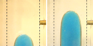
Figure 1. Schematic of a long drop in a circular pipe. The descending fluid (red) moves near the walls with an annular cross-section, the ascending fluid moves near the pipe axis. Here,  $z_d$ and
  $z_a$ are the coordinates of the descending and ascending fronts,
  $\mathcal {L}=z_a-z_d$ is the length of the drop,
  $U_d$ and
  $U_a$ are the front speeds of the two fluids.
Dimensionless relevant parameters are the density ratio  $\mathcal {R}\equiv \rho _a/\rho _d<1$, the Archimedes number
  ${Ar}=\rho _d{\rm \Delta} \rho g R^3/\mu _d^2$, equal to the ratio between buoyancy and viscous forces, the Reynolds number
  ${Re}=(\rho _dR\sqrt {g R {\rm \Delta} \rho /\rho _d})/\mu _d$, the viscosity contrast
 \begin{equation} \mathcal{M}=\frac{\mu_d}{\mu_0(U/R)^{n-1}}\equiv \frac{\mu_d}{\mu_0}\left(\frac{{\rm \Delta} \rho gR}{\mu_d}\right)^{1-n},\end{equation}
i.e. the ratio between the scales of the viscous Newtonian and power-law stresses, and the modified Bingham number for HB fluids
 \begin{equation} {Bm}=\frac{\tau_y}{\mu_0(U/R)^{n}},\end{equation}
the ratio between the yield stress and the scale of the shear component of the tangential stress. Large values of  $\mathcal {M}$ indicate a dominant viscosity in the descending Newtonian fluid, while large values of
  $Bm$ indicate a dominant contribution of the yield stress to the dynamics of the ascending HB fluid.
The mass balance and momentum equations in a cylindrical geometry for the two fluids can be derived in dimensionless form as reported in Appendix A. In particular, if  $\mathcal {M}\gg \varepsilon$, (A11)–(A14) reduce at
  $O (1)$ to
 \begin{align} \left.\begin{array}{@{}ll@{}} \displaystyle \dfrac{1}{\tilde{r}}\dfrac{\partial {}}{\partial {\tilde{r}}}\left(\tilde{r} \dfrac{\partial {\tilde{u}_d}}{\partial {\tilde{r}}}\right) = \dfrac{\partial {\tilde{p}_d}}{\partial {\tilde{z}}} +\dfrac{1}{1-\mathcal{R}}, & \tilde{r}\in[\tilde{\delta},1],\\ \begin{aligned} &\displaystyle\dfrac{1}{\mathcal{M}}\dfrac{1}{\tilde{r}}\dfrac{\partial {}}{\partial {\tilde{r}}} \left(\tilde{r}\left|\dfrac{\partial {\tilde{u}_a}}{\partial {\tilde{r}}}\right|^{n-1} \dfrac{\partial {\tilde{u}_a}}{\partial {\tilde{r}}}\right)\\ &\quad +\,{sgn}\left(\dfrac{\partial {\tilde{u}_a}}{\partial {\tilde{r}}}\right) \dfrac{{Bm}}{\mathcal{M}}\dfrac{1}{\tilde{r}} = \dfrac{\partial {\tilde{p}_a}}{\partial {\tilde{z}}} + \dfrac{\mathcal{R}}{1-\mathcal{R}},\end{aligned} & \textrm{if}\ |{\tau_{rz}}| > \tau_y,\ \tilde{r}\in[0,\tilde{\delta}],\\ \tilde{u}_a=\textrm{const.}, & \textrm{if}\ |{\tau_{rz}}|\le \tau_y,\ \tilde{r}\in[0,\tilde{\delta}],\\ \displaystyle \dfrac{\partial {\tilde{p}_d}}{\partial {\tilde{r}}}=\dfrac{\partial {\tilde{p}_a}}{\partial {\tilde{r}}}=0, \end{array}\right\} \end{align}
for the descending and the ascending fluid, respectively. The symbol  $\widetilde {\cdots }$ indicates a dimensionless variable and
  $\delta$ is the radius of the internal current.
Neglecting the interface tension, the pressure assumes a unique value in the horizontal cross-section for the descending and ascending fluids, 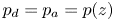 $p_d=p_a=p(z)$, and (2.8) can be written as
 \begin{equation} \left.\begin{array}{@{}ll@{}} \displaystyle \dfrac{1}{{r}}\dfrac{\textrm{d}}{\textrm{d}r} \left({r}\dfrac{\textrm{d}{u}_d} {\textrm{d}{r}}\right) =\underbrace{\dfrac{\textrm{d}p}{\textrm{d}z} +\dfrac{1}{1-\mathcal{R}}}_{\mathcal{P}}, & {r}\in[{\delta},1],\\ \begin{aligned}&\displaystyle\dfrac{1}{\mathcal{M}}\dfrac{1}{r}\dfrac{\textrm{d}}{\textrm{d}{r}} \left({r}\left|\dfrac{\textrm{d}{u}_a}{\textrm{d}{r}}\right|^{n-1} \dfrac{\textrm{d}{u}_a}{\textrm{d}{r}}\right)\\ &\quad +\,{sgn}\left(\dfrac{\textrm{d}{u}_a}{\textrm{d}{r}}\right) \dfrac{{Bm}}{\mathcal{M}}\dfrac{1}{r} = \underbrace{\dfrac{\textrm{d} p}{\textrm{d}z} +\dfrac{\mathcal{R}}{1-\mathcal{R}}}_{\mathcal{P}-1},\end{aligned} & \textrm{if}\ |{\tau_{rz}}| > \tau_y,\ {r}\in[0,{\delta}],\\ u_a=\textrm{const.}, & \textrm{if}\ |{\tau_{rz}}| \le \tau_y,\ {r}\in [0,{\delta}], \end{array}\right\} \end{equation}
where the tilde has been dropped for simplicity. The boundary conditions are
 \begin{equation} \left.\begin{array}{c@{}} u_d(1)=0,\\ u_a(0)\ \textrm{is finite},\\ u_d(\delta)=u_a(\delta),\\ \displaystyle\left.\dfrac{\textrm{d}u_d}{\textrm{d} r}\right|_{r=\delta}= \dfrac{1}{\mathcal{M}}\left|\dfrac{\textrm{d}u_a}{\textrm{d} r}\right|^{n-1}_{r=\delta} \left.\dfrac{\textrm{d}u_a}{\textrm{d} r}\right|_{r=\delta}+ \dfrac{{Bm}}{\mathcal{M}}{sgn}\left(\left.\dfrac{\textrm{d}u_a}{\textrm{d} r}\right|_{r=\delta}\right), \end{array}\right\} \end{equation}
representing (i) the no-slip condition at the wall, (ii) the finiteness of velocity at the axis and the continuity of (iii) velocity and (iv) shear stress  $\tau _{rz}$ at the interface between the two fluids.
Solving the differential problem yields the following velocity profile:
 \begin{align} \left.\begin{array}{ll@{}} u_d(r)=\dfrac{\mathcal{P}}{4}(r^2-1)-\dfrac{\delta ^2}{2}\ln{r}, & {r}\in[{\delta},1],\\ \begin{aligned} u_a(r) & =\dfrac{n}{n+1}\dfrac{[ \mathcal{M} (1-\mathcal{P})\delta-2 Bm ]^{{(n+1)}/{n}}-[\mathcal{M} (1-\mathcal{P}) r-2 Bm ]^{{(n+1)}/{n}}}{ \mathcal{M} (1-\mathcal{P})2^{1/n}}\\ & \quad +\dfrac{\mathcal{P}}{4}(\delta^2-1)-\dfrac{\delta^2}{2}\ln \delta, \end{aligned} & {r}\in[r_y,{\delta}],\\ u_{a({plug})}\equiv u_a(r_y), & {r}\in[0,r_y], \end{array}\right\} \end{align}
where  $\mathcal {P}=\textrm {d}p/\textrm {d}z+1/(1-\mathcal {R})$ is the driving force of the ascending fluid and
  $r_y=2{Bm}/[\mathcal {M}(1-\mathcal {P})]$ is the radius of the axial plug. Imposing a zero net flux at the generic cross-section of the pipe by setting
 \begin{equation} \int_0^\delta 2{\rm \pi} r u_a\,\textrm{d}r+\int_\delta^1 2{\rm \pi} r u_d\,\textrm{d}r=0, \end{equation}
we obtain an equation involving  $\mathcal {M}, Bm, \mathcal {P}, \delta$ and
  $n$, to be solved numerically in order to evaluate
  $\mathcal {P}$.
For the case of a OdW fluid (a HB fluid with null yield stress,  ${Bm}=0$) the ascending and descending velocities reduce to
 \begin{equation} \left. \begin{array}{ll} \displaystyle u_d(r)=\dfrac{\mathcal{P}}{4}(r^2-1)-\dfrac{\delta ^2}{2}\ln{r}, & {r}\in[{\delta},1],\\ \begin{aligned} \displaystyle u_a(r) & =\dfrac{n}{n+1}\left[\dfrac{\mathcal{M} (1-\mathcal{P})}{2}\right]^{{1}/{n}}(\delta^{{(n+1)}/{n}} -r^{{(n+1)}/{n}}) \\ & \quad +\displaystyle\dfrac{\mathcal{P}}{4}(\delta^2-1)- \dfrac{\delta^2}{2}\ln \delta, \end{aligned} & {r}\in[0,{\delta}], \end{array}\right\} \end{equation}
and the zero net flux condition in the generic cross-section, (2.12), becomes
 \begin{equation} \frac{(1-\delta ^4) \mathcal{P}}{8}- \dfrac{n \delta ^{(3n+1)/n}}{(3 n+1) }\left[ \dfrac{\mathcal{M} (1-\mathcal{P})}{2}\right]^{{1}/{n}}- \frac{ \delta ^2 (1-\delta ^2)}{4}=0.\end{equation}
Equation (2.14) admits an analytical solution for  $n=1, 1/2, 1/3, 1/4$ (and for
  $n=2, 3, 4$, a shear-thickening fluid). For
  $n=1$ it results in
 \begin{equation} \mathcal{P}=\delta ^2 \frac{(2 \delta ^2-\delta ^2 \mathcal{M} -2)}{\delta ^4-\delta ^4 \mathcal{M}-1}, \end{equation}
coincident with the solution derived by Picchi et al. (Reference Picchi, Suckale and Battiato2020). For  $n=1/2$ the closed-form solution is
 \begin{equation} \mathcal{P}=1+\dfrac{{5} (1-\delta ^4)}{4 \delta ^5 \mathcal{M}^2}-\dfrac{\sqrt{5}(1-\delta ^2)}{4 \delta ^5 \mathcal{M}^2}{ \sqrt{5 \delta ^4+10 \delta ^2+8 \delta ^5 \mathcal{M}^2+5}}. \end{equation}
The analytical solutions for  $n=1/3, 1/4$ are cumbersome and are not shown; a numerical solution to (2.14) can be derived for any value of the fluid behaviour index.
Figure 2(a) shows the overall driving term  $\mathcal {P}$ as a function of the long drop radius
  $\delta$ and figure 2(b) does the same for the pressure gradient; different values of the viscosity ratio
  $\mathcal {M}$, density ratio
  $\mathcal {R}$ and flow behaviour index
  $n$ are considered. On the one hand, the driving term increases with the drop radius, more rapidly for lower
  $\delta$ values and larger viscosity ratios
  $\mathcal {M}$, until a quasi-linear increase is reached for unit
  $\mathcal {M}$; more shear-thinning fluids determine a more rapid increase of
  $\mathcal {P}$ for larger viscosity ratios, while the influence of rheology is modest for lower viscosity ratios. On the other hand, the pressure gradient increases with the drop radius and also, significantly so, with the density ratio
  $\mathcal {R}$, while it remains largely unaffected by the fluid rheology. Figure 3(a) shows the velocity profiles computed for a Newtonian and a shear-thinning OdW fluid, for different values of
  $\mathcal {M}$ and for
  $\delta =0.6$. Figure 3(b) does the same for the case of an ascending HB fluid, with the presence of a modest plug as a consequence of the non-zero value of
  ${Bm}$ selected; the velocity profile is almost unaffected by the presence of the plug. A backflow of the inner current is observed in both cases as a consequence of the drag of the descending outer current. An increasing viscosity contrast
  $\mathcal {M}$ between the internal and the external fluid determines an increasing backflow in the ascending fluid; shear-thinning fluids show a flattened velocity distribution near the axis, more so for low values of
  $\mathcal {M}$.

Figure 2. An OdW ascending fluid ( $Bm = 0$) and Newtonian descending fluid. (a) Dimensionless
  $\mathcal {P}$ as a function of the long drop radius
  $\delta$ and of the viscosity ratio
  $\mathcal {M}$ for a fluid behaviour index of the ascending fluid
  $n=1,1/2,1/3$; (b) dimensionless pressure gradient as a function of
  $\delta$ and of the density ratio
  $\mathcal {R}$ for
  $\mathcal {M}=10$. The inset shows the domain
  $\delta -\mathcal {M}$ where the
  $\mathcal {P}$ for Newtonian fluid exceeds
  $\mathcal {P}$ for a shear-thinning fluid with
  $n=1/2$ or
  $1/3$: the two curves cannot be distinguished.

Figure 3. Velocity profiles for a generic configuration with  $\delta =0.6$ for different values of the viscosity ratio
  $\mathcal {M}$, and for flow behaviour indexes
  $n=1,0.7$, (a) for OdW fluids (
 ${Bm}=0$) and (b) for HB fluids with
  ${Bm}=0.05$. The thicker part of the curves near the axis indicates the plug.
Figure 4 shows the radius of the plug for different properties of the HB fluids constituting the internal ascending current. The dashed grey area represents the fluid domain subject to shear for a fixed  $Bm$ value: the domain becomes larger for small values of
  $Bm$. The plug radius decreases for increasing
  $Bm$ and for more shear-thinning fluids.

Figure 4. Radius of the plug  $r_y$ as a function of the radius
  $\delta$ of the inner ascending current for different values of its properties
  $n$ and
  $Bm$ and for
  $\mathcal {M}=10$. The grey area represents the shearing zone for a HB fluid with
  $Bm=1$.
The shear stress at the interface is shown in figure 5 as a function of the interface position  $\delta$ for different values of
  $Bm$ and
  $n$ of the ascending inner fluid and a fixed viscosity ratio. The (negative) shear stress decreases with increasing
  $\delta$, reaches a minimum and then increases to zero for
  $\delta =1$. Conversely, for a given
  $\delta$ the magnitude of the tangential stress increases with
  $Bm$ and is greater for shear-thinning than for Newtonian fluids.

Figure 5. Tangential stress at  $r=\delta$, the interface between the inner and the outer current, as a function of the fluid behaviour index
  $n$ and of the Bingham number
  $Bm$ of the inner ascending fluid, for
  $\mathcal {M}=10$.
Figures 6(a) and 6(b) show the velocity and the tangential stress profiles for an ascending non-Newtonian fluid with zero (OdW) and non-zero (HB) yield stress, respectively. A backflow occurs in both cases, with the non-Newtonian fluid dragged down by the Newtonian one at their interface, while a plug is evident for the HB fluid. The velocity profiles associated with the HB fluid are flatter due to the presence of the plug. The tangential stress shows a linear behaviour, attaining the minimum value at the drop radius, the maximum value at the outer wall and a null value where the downward Newtonian velocity is larger in absolute value.

Figure 6. Velocity profiles (blue hatched) and tangential stress (green hatched) radial distributions for a Newtonian descending fluid and (a) an OdW ascending shear-thinning fluid ( ${Bm}=0$) and (b) a HB ascending fluid (
 ${Bm}=0.2$). The parameter values are
  $n=0.5, \mathcal {M}=10, \delta =0.6$.
The average ascending and descending speed of the long drop is obtained by averaging the velocity profiles (2.11) along the cross-section
 \begin{equation} U_a=\dfrac{1}{{\rm \pi}\delta^2}\int_0^\delta 2{\rm \pi} ru_a(r)\,\textrm{d}r, \quad U_d=\dfrac{1}{{\rm \pi}(1-\delta^2)}\int_\delta^12{\rm \pi} r u_d(r) \,\textrm{d}r. \end{equation}
 Since the zero net flux condition, (2.12), can be written as  $U_aA_a+U_dA_d=0$, this gives
 \begin{equation} U_a={-}\dfrac{A_d}{A_a}U_d=\dfrac{\delta^2-1}{\delta^2}U_d. \end{equation}
 Figure 7 shows the speed of the ascending and descending fronts as a function of the long drop radius  $\delta$ and of the viscosity contrast
  $\mathcal {M}$ for an ascending fluid that is Newtonian (
 $n=1$) and shear-thinning OdW fluid (
 ${Bm}=0$) with
  $n=1/2, 1/3$. It is seen that the speed of the ascending fluid depends on the long drop radius in a non-monotonic fashion, first increasing from zero, reaching a maximum and then decreasing towards zero as
  $\delta$ goes from zero to unity. The ascent speed strongly increases for a large viscosity contrast
  $\mathcal {M}$ until
  $\delta <0.8$, while it is modestly affected by the fluid rheology. The downward speed of the descending Newtonian fluid shows a similar behaviour, except the influence of the rheology of the ascending fluid is relatively more impactful. Further, the
  $n$-index modulates the speed, and it can happen that a current with
  $n<1$ shows a higher ascent speed than one with
  $n=1$. To exemplify this case, figure 8 shows the
  $\delta -\mathcal {M}$ shaded domain where an OdW ascending fluid with
  $n=1/2$ or
  $1/3$ generates a long drop faster than a HB ascending fluid with
  $n=1$ and
  $Bm = 0.0, 0.1, 1.0$. The domain is almost rectangular with
  $\delta$ ranging from
  $0.05$ to
  $0.55$ for
  $\mathcal {M}>80$, while its width narrows for
  $\mathcal {M}<80$, until at
  $\mathcal {M}\approx 10.4$ for both
  $n=1/2$ and
  $1/3$, the required condition is satisfied only for a single value,
  $\delta =0.32$. Increasing
  $Bm$ results in a shrinking of the domain.

Figure 7. Long drop average speed for an OdW ascending fluid ( ${Bm}=0$). (a) Ascent speed and (b) descent speed as a function of the long drop radius
  $\delta$ and the viscosity ratio
  $\mathcal {M}$ for
  $n=1,1/2,1/3$.

Figure 8. Ranges  $\delta$–
 $\mathcal {M}$ where the ascent speed for an OdW fluid with
  $n=1/2$ and
  $n=1/3$ is larger than the ascent speed for a HB fluid with
  $n=1$ and
  ${Bm}=0, 0.1, 1$.
The limit condition  $\mathcal {M}\rightarrow \infty$ is equivalent to a descending Newtonian fluid having a viscosity much larger than the viscosity (for a Newtonian ascending fluid) or the apparent viscosity (for a HB ascending fluid) of the inner current. The asymptotic speeds are
 \begin{equation} \left. \begin{array}{l@{}} U_d(\delta,\mathcal{M}\rightarrow\infty,{Bm},n)={-} \dfrac{\delta^4(3-4\ln\delta)+1-4\delta^2}{8(1-\delta^2)},\\ U_a(\delta,\mathcal{M}\rightarrow\infty,{Bm},n)= \dfrac{\delta^4(3-4\ln\delta)+1-4\delta^2}{8\delta^2}, \end{array}\right\} \end{equation}
and do not depend on  ${Bm}$ or the fluid behaviour index
  $n$. This result was expected, since in (2.9), the limit
  $\mathcal {M}\to \infty$, with finite
  $Bm$, leads to the condition
  $\mathcal {P}=1$ with the homogeneous boundary condition
  $\textrm {d}u_d/\textrm {d}r=0$ at
  $r=\delta$, which allows integration of the velocity profile of the Newtonian descending current without involving any rheological parameter of the ascending fluid. When
  $\mathcal {M}\to \infty$ and
  $Bm$ is of the same order as
  $\mathcal {M}$, the boundary conditions for the descending fluid reduces to
  $\textrm {d}u_d/\textrm {d}r=- Bm /\mathcal {M}$ at
  $r=\delta$, and the asymptotic speeds are
 \begin{align} \left. \begin{array}{l@{}} U_d(\delta,\mathcal{M}\rightarrow\infty,{Bm}=O(\mathcal{M}),n) ={-}\dfrac{\delta^4(3-4\ln\delta)+1-4\delta^2}{8(1-\delta^2)}+ \dfrac{Bm}{\mathcal{M}}\dfrac{1-\delta^2}{8\delta},\\ U_a(\delta,\mathcal{M}\rightarrow\infty,{Bm}=O(\mathcal{M}),n) =\dfrac{\delta^4(3-4\ln\delta)+1-4\delta^2}{8\delta^2}- \dfrac{Bm}{\mathcal{M}}\dfrac{(1-\delta^2)^2}{8\delta^3}, \end{array}\right\} \end{align}
with the descending current slowed by the tangential stress at the interface of the ascending internal plug. Equations (2.20) are valid only for the  $\delta$ values that make the average speed for the descending and ascending current negative and positive, respectively.
The other limit of interest  $\mathcal {M}\rightarrow 0$ corresponds to a rigid plug, and the speeds are
 \begin{align} \left. \begin{array}{l@{}} U_d(\delta,\mathcal{M}\rightarrow 0,{Bm}=0,n)={-} \dfrac{\delta^4(\delta^2-1-\ln\delta-\delta^2\ln\delta)}{2(1-\delta^4)},\\ U_a(\delta,\mathcal{M}\rightarrow 0,{Bm}=0,n)= \dfrac{\delta^2(\delta^2-1-\ln\delta-\delta^2\ln\delta)}{2(\delta^2+1)}, \end{array}\right\} \end{align}
again independent on the fluid behaviour index  $n$. Note that, for
  $\mathcal {M} \to 0$, the limiting radius of the plug tends to infinity unless
  $Bm = 0$ since
  $r_y=2 Bm /(\mathcal {M}(1-\mathcal {P}))$ with
  $\mathcal {P}< 1$, so the latter limit condition is only valid for an OdW fluid with
  $Bm=0$.
For  $\mathcal {M}=O(1)$ and
  $Bm$ sufficiently large, the ascending current is all plug, with
  $\mathcal {P}\to 2\delta ^2/(1+\delta ^2)$. The condition
  $r_y=\delta$ is reached for
  ${Bm}=\mathcal {M}\delta (1-\delta ^2)/(2+2\delta ^2)$, with a maximum value
  ${Bm}\approx 0.15\mathcal {M}$, so for
  $Bm$ not particularly large. The asymptotic speeds are again those in (2.21).
A more in-depth analysis of the asymptotic ascending speed for  $\mathcal {M} \to 0$ and
  $\mathcal {M} \to \infty$, and of the corresponding flow rate, is reported in § 5.
3. The Ellis model for the inner ascending current
In the previous section, the HB model adopted for the ascending fluid reduces to the OdW model for  $Bm=0$. Now the OdW model typically shows an inconsistency: the apparent viscosity tends to infinity for shear rates tending to zero (see e.g. Myers Reference Myers2005). In order to eliminate this inconsistency and to adapt the rheological model to the effective experimental behaviour of shear-thinning fluids, we adopt the three-parameter Ellis model, which has been extensively and successfully applied to describe the flow in complex geometries (Al-Behadili et al. Reference Al-Behadili, Sellier, Hewett, Nokes and Moyers-Gonzalez2019; Ali et al. Reference Ali, Hussain, Ullah and Bég2019; Celli, Barletta & Brandão Reference Celli, Barletta and Brandão2021; Ciriello et al. Reference Ciriello, Lenci, Longo and Di Federico2021; Picchi et al. Reference Picchi, Ullmann, Brauner and Poesio2021). The Ellis model relates the apparent viscosity to the stress tensor as
 \begin{equation} \eta=\dfrac{\eta_0}{1+\left(\dfrac{{{{\boldsymbol{\tau: \tau}}}}}{2\tau_0^2}\right)^{(\alpha-1)/2}}, \end{equation}
where  $\tau _0$ is the shear stress corresponding to an apparent viscosity
  $\eta _0/2$ and
  $\alpha \ge 1$ for a shear-thinning fluid is an indicial parameter. The apparent viscosity tends to 0 for
  $\tau _0\to 0$ and
  $\alpha >1$ and tends to
  $\eta _0/2$ for
  $\alpha \to 1$. For intense shear stress
  $\tau \gg \tau _0$ the apparent viscosity reduces to
 \begin{equation} \eta=\eta_0\left(\dfrac{\tau}{\tau_0}\right)^{1-\alpha}\quad \alpha\ne 1, \end{equation}
and the fluid behaves as an OdW power law with  $\alpha =1/n$ and a consistency factor
  $\mu _0=\eta _0^n\tau _0^{1-n}$. For
  $\alpha =1$ the fluid is Newtonian with
  $\eta =\eta _0/2$.
With the same approximations adopted for an ascending HB fluid, the balance of linear momentum in the vertical direction reads
 \begin{equation} \dfrac{1}{\mathcal{M'}}\dfrac{\partial \tilde{u}_a}{\partial \tilde{r}}=\left(\underbrace{\dfrac{\partial {\tilde{p}_a}}{\partial {\tilde{z}}} + \dfrac{\mathcal{R}}{1-\mathcal{R}}}_{\mathcal{P}-1}\right) \left[1+\beta\left|\underbrace{\dfrac{\partial {\tilde{p}_a}}{\partial {\tilde{z}}} +\dfrac{\mathcal{R}}{1-\mathcal{R}}}_{\mathcal{P}-1}\right|^{\alpha-1} \left(\dfrac{\tilde{r}}{2}\right)^{\alpha-1}\right] \dfrac{\tilde{r}}{2},\quad \tilde{r}\in[0,\tilde{\delta}], \end{equation}
where a second viscosity ratio
 \begin{equation} \mathcal{M'}=\dfrac{\mu_d}{\eta_0},\end{equation}
was introduced, and the parameter
 \begin{equation} \beta=\left(\dfrac{{\rm \Delta} \rho\,g R}{\tau_0}\right)^{\alpha-1},\end{equation}
measures the relative importance of buoyancy and the typical shear stress of an Ellis fluid. The boundary conditions are
 \begin{equation} \left. \begin{array}{c@{}} u_d(1)=0,\\ u_a(0)\ \textrm{is finite},\\ u_d(\delta)=u_a(\delta),\\ \left.\dfrac{\textrm{d}u_a}{\textrm{d} r}\right|_{r=\delta} =\mathcal{M}'\left[1+\beta\left|\left.\dfrac{\textrm{d}u_d}{\textrm{d} r}\right|_{r=\delta}\right|^{\alpha-1}\right] \left.\dfrac{\textrm{d}u_d}{\textrm{d} r}\right|_{r=\delta}, \end{array}\right\} \end{equation}
with the same meaning as (2.10) and where the tilde has been dropped.
Solving the differential problem, we calculate the following velocity profiles:
 \begin{equation} \left. \begin{array}{ll@{}} u_d(r)=\dfrac{\mathcal{P}}{4}(r^2-1)-\dfrac{\delta ^2}{2}\ln{r} , & {r}\in[{\delta},1],\\ \begin{aligned} u_a(r) & =\mathcal{M}'(1-\mathcal{P})\dfrac{\delta^2-r^2}{4}+\mathcal{M}' \beta(1-\mathcal{P})^\alpha\dfrac{\delta^{\alpha+1}-r^{\alpha+1}}{2^\alpha (\alpha+1)} \\ & \quad+\dfrac{\mathcal{P}}{4}(\delta^2-1)- \dfrac{\delta^2}{2}\ln \delta,\end{aligned} & {r}\in[0,{\delta}],\\ \end{array}\right\} \end{equation}
where we have assumed  $\mathcal {P}<1$ for physical consistency. For
  $\tau _{rz}\gg \tau _0$ (3.7) simplify as follows:
 \begin{equation} \left. \begin{array}{ll@{}} u_d(r)=\dfrac{\mathcal{P}}{4}(r^2-1)-\dfrac{\delta ^2}{2}\ln{r} , & {r}\in[{\delta},1],\\ \begin{aligned} u_a(r) & \approx\mathcal{M}'\beta(1-\mathcal{P})^\alpha \dfrac{\delta^{\alpha+1}-r^{\alpha+1}}{2^\alpha(\alpha+1)} \\ & \quad+\dfrac{\mathcal{P}}{4}(\delta^2-1)- \dfrac{\delta^2}{2}\ln \delta, \end{aligned} & {r}\in[0,{\delta}], \end{array}\right\} \end{equation}
which upon substituting  $\alpha =1/n$ and
  $\mu _0=\eta _0^n\tau _0^{1-n}$ collapse to (2.13) valid for an OdW fluid.
Figure 9 shows the velocity profiles computed for an ascending Ellis fluid, for different values of  $\mathcal {M}',\beta,\alpha$ and for
  $\delta =0.6$. The profiles are qualitatively similar to those for an OdW fluid, with a backflow of the inner current due to the drag of the outer current; the backflow is accentuated as the buoyancy dominates over the typical shear stress of an Ellis fluid (larger
  $\beta$). More shear-thinning fluids (larger
  $\alpha$) exhibit flatter velocity profiles and hence less backflow. An increasing viscosity contrast
  $\mathcal {M}'$ reduces the differences between velocity profiles for different values of
  $\beta$ and
  $\alpha$.

Figure 9. Ellis ascending fluid and Newtonian descending fluid. Velocity profiles for a generic configuration with  $\delta =0.6$, different values of the ratio
  $\beta, \alpha =2,3$ and (a)
  $\mathcal {M}'=1$ and (b)
  $\mathcal {M}'=10$.
The average speeds of the descending outer current and of the ascending inner current are
 \begin{equation} \left. \begin{array}{c@{}} U_d=\dfrac{1}{8(1-\delta^2)}[2\delta^2(1-\delta^2+2\delta^2\ln\delta)- (1-\delta^2)^2\mathcal{P}],\\ U_a=\dfrac{ \mathcal{M}' \beta\delta ^{\alpha +1} (1- \mathcal{P})^{\alpha }}{2^{\alpha }(\alpha +3)}+\dfrac{1}{8} \mathcal{M}'\delta ^2 (1-\mathcal{P})-\dfrac{1}{4} [2 \delta ^2 \ln\delta+ \mathcal{P}(1-\delta^2)], \end{array}\right\} \end{equation}
and the corresponding flow rates are  $Q_d={\rm \pi} (1-\delta ^2)U_d, Q_a={\rm \pi} \delta ^2U_a$.
Figure 10 shows the average speed as a function of the long drop radius  $\delta$, of the ratio of scale stresses
  $\beta$, of the viscosity ratio
  $\mathcal {M}'$ for Ellis shear-thinning fluids with
  $\alpha =2, 3$ and
  $\beta =10,100,1000,10\,000$. As for OdW and HB fluids, the ascent speed peaks at an intermediate value of the long drop radius; further, it is strongly impacted by the
  $\beta$ value, and significantly decreases with increasing shear-thinning behaviour, especially in the low range of
  $\delta$. A similar behaviour is shared by the Newtonian descent speed, except the absolute values of the speed are lower.

Figure 10. Long drop speeds for an Ellis ascending fluid and a Newtonian descending fluid. (a) Ascent speed and (b) descent speed as a function of the long drop radius  $\delta$ and the ratio
  $\beta$ for
  $\alpha =2,3, \mathcal {M}'=10$.
By imposing  $Q_a+Q_d=0$, an equation in
  $\mathcal {P},\mathcal {M}',\beta,\alpha,\delta$ is obtained, which may be used to calculate the driving term
  $\mathcal {P}$ for given values of the other parameters. The equation admits analytical solutions for
  $\alpha =1,2,3,4$, and requires a numerical solution for other values of
  $\alpha$.
The asymptotic velocities for  $\mathcal {M}'\to \infty$ and for
  $\mathcal {M}'\to 0$ collapse to (2.19) and to (2.21), respectively, and are independent of
  $\beta$.
A more in-depth analysis of the asymptotic ascending speed for  $\mathcal {M}' \to 0$ and
  $\mathcal {M}' \to \infty$, and of the corresponding flow rate, is reported in § 5.
4. The energy balance for a Newtonian descending fluid and a HB or Ellis ascending fluid
The present section formulates the energy balance for the non-Newtonian ascending Taylor drop; the balance is valid after enough time has elapsed from its formation, allowing the drop to elongate so that the validity of the lubrication approximation previously employed is ensured. The ascending drop gains energy in potential form, loses energy due to viscous dissipation and stores some energy as kinetic energy of the two counter-current fluids. Neglecting the work performed by the forces at the interfaces, the balance is between kinetic energy  $\mathcal {E}_k$, potential energy
  $\mathcal {E}_p$ and viscous dissipation
  $\varPhi$ according to (Picchi et al. Reference Picchi, Suckale and Battiato2020)
 \begin{equation} \dfrac{\textrm{d}\mathcal{E}_k}{\textrm{d}t}+ \dfrac{\textrm{d}\mathcal{E}_p}{\textrm{d}t}+\varPhi=0,\end{equation}
written in dimensional form. The corresponding scales are  $\mathcal {E}_k \sim \rho _d U^2 \mathcal {L}R^2, \mathcal {E}_p\sim (\rho _d-\rho _a) g\mathcal {L}^2R^2$ and
  $\varPhi \sim \mu _dU^2\mathcal {L}$, hence (4.1) can be written in dimensionless variables as
 \begin{equation} \dfrac{1}{{Ri}(1-\mathcal{R})}\dfrac{\textrm{d} \tilde{\mathcal{E}}_k}{\textrm{d}\tilde{t}}+\dfrac{1}{1-\mathcal{R}} \dfrac{\textrm{d}\tilde{\mathcal{E}}_p}{\textrm{d}\tilde{t}} +\tilde{\varPhi}=0,\quad {Ri}=1/[({1-\mathcal{R}})\varepsilon {Ar}], \end{equation}
where  ${Ri}$ is the Richardson number expressing the ratio between potential and kinetic energy. For the special case
  ${Ri}\to \infty$ considered hereinafter the kinetic energy variation is negligible and (4.2) reduces to
 \begin{equation} \dfrac{\textrm{d}\tilde{\mathcal{E}}_p}{\textrm{d}\tilde{t}}={-}(1-\mathcal{R})\tilde{\varPhi}.\end{equation}
The potential energy in (4.1) is computed by integration over the drop region and is equal to
 \begin{align} \mathcal{E}_p&=\rho_dg{\rm \pi}\left[(R^2-\delta^2)\int_{z_d}^{z_a}z\,\textrm{d} z+R^2\int_{z_a}^{L}z\,\textrm{d} z\right]\nonumber\\ &\quad +\rho_ag{\rm \pi}\left[\delta^2\int_{z_d}^{z_a}z\,\textrm{d} z+R^2\int^{z_d}_{{-}L}z\,\textrm{d} z\right]. \end{align}
In dimensionless form the potential energy results in
 \begin{equation} \tilde{\mathcal{E}}_p=\tfrac{1}{2}{\rm \pi}[(1-\tilde{\delta}^2) \tilde{U}_d^2-\tilde{\delta}^2\tilde{U}_a^2] \tilde{t}^{\,2}+\textrm{const.}, \end{equation}
or equivalently
 \begin{equation} \mathcal{E}_p=\dfrac{2\delta^2-1}{2{\rm \pi}\delta^2(1-\delta^2)} Q_a^2t^2+\textrm{const.}, \end{equation}
where  $Q_a$ is the flow rate of the ascending current, also defined as the transport number
  $Te$ (see Huppert & Hallworth Reference Huppert and Hallworth2007), and the tilde symbol is omitted for simplicity.
The dissipation rate is computed as
 \begin{equation} \varPhi=\int_{\mathcal{V}_d}({{\boldsymbol{\tau:}\boldsymbol{\mathsf{D}}}})_d\, \textrm{d}\mathcal{V}+\int_{\mathcal{V}_a}({{\boldsymbol{\tau:}\boldsymbol{\mathsf{D}}}})_a \,\textrm{d}\mathcal{V}, \end{equation}
where  $\mathcal {V}_{a,d}$ refers to the volume of ascending lighter/descending denser fluid.
In a cylindrical geometry and under a HB rheology for the internal current one has
 \begin{equation} \varPhi\equiv\varPhi_d+\varPhi_a=2{\rm \pi}\mathcal{L}(t)\left\{\mu_d \int_{\delta}^R \left(\dfrac{\textrm{d}u_d}{\textrm{d} r}\right)^2 \,\textrm{d}r +\int_{0}^\delta \left[\mu_0\left|\dfrac{\textrm{d} u_a}{\textrm{d} r}\right|^{n+1}+\tau_y\left|\dfrac{\textrm{d} u_a}{\textrm{d} r}\right|\right]\,\textrm{d}r\right\}, \end{equation}
or in dimensionless form
 \begin{equation} \tilde{\varPhi}\equiv\tilde{\varPhi}_d+\tilde{\varPhi}_a= 2{\rm \pi}\tilde{\mathcal{L}}(\tilde{t})\left\{\int_{\tilde{\delta}}^1 \left(\dfrac{\textrm{d}\tilde{u}_d}{\textrm{d} \tilde{r}} \right)^2\textrm{d}\tilde{r} +\dfrac{1}{\mathcal{M}} \int_{0}^{\tilde{\delta}} \left[\left|\dfrac{\textrm{d} \tilde{u}_a}{\textrm{d} \tilde{r}}\right|^{n+1}+{Bm} \left|\dfrac{\textrm{d}\tilde{u}_a}{\textrm{d} \tilde{r}} \right|\right]\,\textrm{d}\tilde{r}\right\}.\end{equation}
Upon integration using (2.11), (4.9) transforms into
 \begin{equation} \left. \begin{array}{c} \varPhi_d = 2{\rm \pi}(U_a-U_d)\left\{ \dfrac{\rm \pi}{8}\mathcal{P} [(1-\delta^4)\mathcal{P}-4\delta^2(1-\delta^2)]- \dfrac{\rm \pi}{2}\delta^4\ln\delta\right\}t, \\ \begin{aligned} \varPhi_a & = 2{\rm \pi}(U_a-U_d)\left\{\dfrac{{\rm \pi} n[\delta \mathcal{M}(1- \mathcal{P})-2 Bm ]^{(2n+1)/n} [2n Bm +\delta \mathcal{M} (2 n+1)(1-\mathcal{P})]}{ 2^{1/n}\mathcal{M}^3 (6 n^2+5 n+1) (1-\mathcal{P})^2}\right.\\ & \quad+\left.\dfrac{ {\rm \pi} Bm [ Bm +\delta \mathcal{M}(1-\mathcal{P})] [2 Bm -\delta \mathcal{M}(1-\mathcal{P})]^2}{3 \mathcal{M}^3 (1-\mathcal{P})^2}\right\}t, \end{aligned} \end{array}\right\} \end{equation}
where the symbol  $\widetilde {\cdots }$ is omitted for simplicity, and where
  $\mathcal {L}(t)=(U_a-U_d)t$ is the time varying length of the drop. This suggests an alternative formulation of (4.9) as
 \begin{equation} \varPhi=Q_a(U_a-U_d)t\equiv \dfrac{Q_a^2}{{\rm \pi}\delta^2(1-\delta^2)}t, \end{equation}
clarifying that, in dimensionless form, the dissipation rate per unit length is equal to the flow rate. Figure 11 depicts the dissipation rate per unit length  $\varPhi /\mathcal {L}$ for two different viscosity ratios and several combinations of ascending fluids. The dissipation rate is zero at
  $\delta =0,1$ and peaks at an intermediate value of
  $\delta$ in all cases. A higher total dissipation rate is attained for a larger viscosity ratio, while shear-thinning effects decrease or increase the total dissipation rate with respect to the Newtonian case
  $n=1$ depending on the value of the viscosity ratio. The appearance of a non-zero yield stress induces a lower total dissipation rate for many combinations of viscosity ratio and fluid behaviour index, while for other combinations the total dissipation rate is practically unchanged. There exists a complex interplay between shear rate and shear stress, so it cannot be immediately established which of the two terms is more affected by the presence of yield stress (non-zero
  $Bm$) and by the value of the viscosity ratio.

Figure 11. Dissipation rate per unit length  $\varPhi /\mathcal {L}$ as a function of
  $\delta$ for
  $\mathcal {M}=1,10^3, n=0.5,1.0$ and
  ${Bm}=0.0,0.1, 1.0$. The continuous curves refer to an OdW ascending fluid (
 $Bm = 0.0$), the dashed curves to
  $Bm = 0.1$ and the dot-dashed curves to
  $Bm = 1.0$ The red curves refer to the ascending HB or OdW current, the blue curves to the descending Newtonian current, the black curves are the total dissipation. For
  $\mathcal {M}=1$ only curves for
  $Bm = 0.1$ can be drawn, since for
  $Bm = 1.0$ it is always
  $\delta < r_y$.
Looking now at the individual contributions of the ascending and descending currents to the total dissipation rate, it is seen that the contribution of the ascending current depends on the viscosity ratio, fluid behaviour index and modified Bingham number, but tends to be smaller than that of the descending Newtonian current in most cases.
The maximum dissipation rate is attained for intermediate values of  $\delta$ in all cases. Figure 12 shows the maximum dissipation rate and the corresponding radius of the ascending internal current,
  $\delta _{{max}}$, vs
  $\mathcal {M}$. The maximum dissipation rate increases with the viscosity contrast, while the opposite is true for the corresponding radius. Both results moderately depend on the fluid behaviour index, with values in a range limited by the condition
  $\delta >r_y$. A modest dependence on the modified Bingham number is evident only for the maximum dissipation rate and not for the corresponding radius.

Figure 12. Maximum dissipation rate (coincident with maximum flow rate) per unit length  $\varPhi /\mathcal {L}$ and corresponding radius of the internal ascending current as a function of
  $\mathcal {M}$. The continuous curves refer to an OdW ascending fluid (
 $Bm = 0.0$), the dashed and dot-dashed curves refer to a HB ascending fluid with
  $Bm = 0.1, 1.0$, respectively.
We have now the expressions of the terms involved in the energy balance, (4.3), and since  $\mathcal {E}_p=f(\delta (t),n,\mathcal {M},{Bm},t)$, (4.3) can be written as
 \begin{equation} \dfrac{\partial \mathcal{E}_p}{\partial \delta}\dfrac{\textrm{d} \delta}{\textrm{d}t}+\dfrac{\partial \mathcal{E}_p}{\partial t}={-}(1-\mathcal{R})\varPhi, \end{equation}
or
 \begin{align} \dfrac{\textrm{d}\delta}{\textrm{d}t}=\dfrac{-(1-\mathcal{R})\varPhi- \dfrac{\partial \mathcal{E}_p}{\partial t}}{\dfrac{\partial \mathcal{E}_p}{\partial \delta}}\equiv{-}\dfrac{\delta(1-\delta^2)(\mathcal{R}-2\delta^2)}{-(1- 2\delta^2+2\delta^4)+\delta(1-3\delta^2+2\delta^4)\dfrac{\partial \ln Q_a}{\partial \delta}}\dfrac{1}{t},\end{align}
which describes the time evolution of the radius of the ascending current, impacted by rheology via the flow rate  $Q_a$. Figure 13 shows the evolution of the current by integrating (4.13) with different initial conditions for a given OdW fluid. For
  $\mathcal {M}=1$, initial conditions within the yellow band evolve into the asymptotic value
  $\delta _{3\infty }=\sqrt {2\mathcal {R}}/2$; slightly different results are obtained for finite values of
  $\mathcal {M}$, including
  $\mathcal {M}\to 0$; the two physically meaningless asymptotes
  $\delta _{1\infty }=0$ and
  $\delta _{2\infty }=1$ are reached for initial conditions out of the yellow band. For other
  $\mathcal {M}$ values, the width of the band varies. For
  $\mathcal {M}\to \infty$ the asymptotic value
  $\delta _{1\infty }=0$ is missing, and the domain of attraction of
  $\delta _{3\infty }$ is larger. The results for a HB ascending fluid (not shown) are very similar, except for the case
  $\mathcal {M}\to \infty$, which implies again the existence of the asymptotic solution
  $\delta _{1\infty }$. Note that, for a HB ascending fluid, the model requires that
  $\delta >r_y$.

Figure 13. Time evolution of the radius of the internal ascending current for  $n=0.5, \mathcal {R}=0.8, {Bm} = 0.0$ and (a)
  $\mathcal {M}=1$, (b)
  $\mathcal {M}\to \infty$.
Figure 14 depicts the time derivative of the radius of the ascending current, the right-hand side of (4.13), at a given time for  $\delta \in [0,1]$ and different values of
  $\mathcal {M}$, for a shear-thinning OdW or HB fluid. For finite values of
  $\mathcal {M}$ there are three stable nodes for
  $\delta _{1\infty }=0, \delta _{2\infty }=1$ and
  $\delta _{3\infty }=\sqrt {2\mathcal {R}}/2$, albeit the first two are physical meaningless. It is noteworthy that similar results were obtained by Picchi et al. (Reference Picchi, Suckale and Battiato2020) for Newtonian ascending fluids. The domain of attraction of the stable node
  $\delta _{3\infty }$ depends mainly on
  $\mathcal {M}$, see figure 15 where the domain of attraction is shown for different values of the fluid behaviour index
  $n$ and for an OdW or HB fluid. The shear-thinning behaviour favours moderately larger bandwidths, whereas the effect of the yield stress is generally modest.

Figure 14. Evolution of the radius of the internal ascending current at  $t=0.1$ for
  $n=0.5, \mathcal {R}=0.8, {Bm} = 0$, and (a)
  $\mathcal {M}=0$, (b)
  $\mathcal {M}=1$, (c)
  $\mathcal {M}\to \infty$. The grey curves refer to a HB fluid with
  ${Bm}=0.1$, and can be drawn only in the domain
  $\delta >r_y$. The latter condition is never satisfied for
  $\mathcal {M}=0$ (a), is always satisfied for
  $\mathcal {M}\to \infty$ (b) and is satisfied in a limited range of
  $\delta$ for
  $\mathcal {M}=1$ and
  ${Bm}=0.1$ (c). The red curves refer to a HB fluid with
  ${Bm}=1$, and can be drawn only in the domain
  $\delta >r_y$, which is empty for
  $\mathcal {M}=0, 1$ and is non-empty only for large
  $\mathcal {M}$.

Figure 15. Domain of attraction of the stable node  $\delta _{3\infty }=\sqrt {2\mathcal {R}}/2$ for
  $n=1,1/2,1/3, \mathcal {R}=0.8, {Bm} = 0$ (OdW fluid). The grey curves, more evident in the enlargement below, refer to a HB fluid with
  ${Bm} = 0.1$ (thick grey) and to
  ${Bm} = 1.0$ (thin grey), the blue dashed and dot-dashed curves represent the condition
  $\delta >r_y$ for
  ${Bm} = 0.1, 1.0$, respectively. The vertical arrows indicate the direction of evolution over time of the radius of the ascending current towards the stable node
  $\delta _{3\infty }=\sqrt {2\mathcal {R}}/2$.
If the ascending fluid is modelled according to the Ellis model, the dimensionless dissipation rate is computed as
 \begin{align} \varPhi\equiv\varPhi_d+\varPhi_a=\mathcal{L}(t)\left[\int_{\delta}^1 2{\rm \pi}\left(\dfrac{\textrm{d}u_d}{\textrm{d} r}\right)^2r\, \textrm{d}r+\int_{0}^\delta 2{\rm \pi}\mathcal{M}'(\tau_{rz}^2+ \beta|\tau_{rz}|^{\alpha+1})r\,\textrm{d}r\right], \end{align}
resulting in
 \begin{equation} \left. \begin{array}{c@{}} \varPhi_d = 2{\rm \pi}(U_a-U_d)\left\{ \dfrac{\rm \pi}{8}\mathcal{P} [(1-\delta^4)\mathcal{P}-4\delta^2(1-\delta^2)]- \dfrac{\rm \pi}{2}\delta^4\ln\delta\right\}t, \\ \varPhi_a= 2{\rm \pi}(U_a-U_d) \left[\dfrac{8 \beta \delta ^{3+ \alpha} }{\alpha +3}| 1-\mathcal{P}|^{\alpha +1}+2^{\alpha } \delta^4 (1-\mathcal{P})^2\right]\dfrac{{\rm \pi}\mathcal{M}'}{2^{\alpha +3}}t. \end{array}\right\} \end{equation}
 The dimensionless dissipation rate is again expressed as a function of the flow rate of the ascending current, see (4.11). The time evolution of the radius of the internal current is identical to (4.13), only the expression of  $Q_a$ changes as a consequence of the different rheological model. When compared, the results are similar to those obtained for the subcase of power-law fluid (not shown). It is important to point out that the asymptotic value
  $\delta _{3\infty }$ does not depend on the rheological behaviour of the ascending fluid, but only on
  $\mathcal {R}$.
5. The asymptotic ascending speed and flow rate
Adopting the HB model or the Ellis model for the inner ascending current, it is seen that its ascent speed has two plateaus for  $\mathcal {M}\,(\mathcal {M}')\to 0$ and for
  $\mathcal {M}\,(\mathcal {M}')\to \infty$, where it becomes only a function of its radius. Figures 16 and 17 show the curves corresponding to zero and non-zero yield stress for different values of the fluid behaviour index and two different ratios of buoyancy to Ellis shear stress
  $\beta$ for different values of the indicial parameter
  $\alpha$, respectively. For both rheologies, the asymptotic value is reached more quickly for less shear-thinning behaviour, without yield stress (
 ${Bm}=0)$ for the HB fluid and larger
  $\beta$ for the Ellis fluid. The insets show the values of
  $\mathcal {M},\mathcal {M}'$ above which 95 % of the asymptotic ascent speed is reached, as a function of
  $n,{Bm}$ or
  $\alpha,\beta$. The asymptotic values of the viscosity ratio are an increasing function of
  ${Bm}$ and a decreasing function of
  $\beta$. For
  $\mathcal {M}>150$ or
  $\mathcal {M}'>50$, one can assume the asymptote is always reached irrespective of the other parameters (except
  $\mathcal {R}$ that is included in
  $\delta _{3\infty }$); by interpolating the numerical values of the asymptotic velocity computed for several combinations
  $\mathcal {R}-\mathcal {M}$ in the range
  $0.5<\mathcal {R}<1$ and
  $\mathcal {M}>150$ (or
  $\mathcal {M}'>50$), the ascent speed and the corresponding flow rate can be approximated as
 \begin{equation} \left. \begin{array}{@{}l} U_a\approx 1.34\exp({-}4\mathcal{R})\\ Q_a\equiv Te \approx2.1\mathcal{R}\exp({-}4\mathcal{R}) \end{array}\quad \textrm{for}\ \mathcal{M}>150(\mathcal{M}'>50) \ \textrm{and}\ 0.5<\mathcal{R}<1,\right\}\end{equation}
where a negative exponential function of the density ratio  $\mathcal {R}$ was adopted for interpolation. Equation (5.1) becomes in dimensional variables
 \begin{align} \left. \begin{array}{@{}l} {U}_a\approx 1.34\exp({-}4\mathcal{R})\dfrac{{\rm \Delta} \rho\,gR^2}{\mu_d}\\ {Q}_a\approx 2.1\mathcal{R}\exp({-}4\mathcal{R}) \dfrac{{\rm \Delta} \rho\,gR^4}{\mu_d}\end{array} \quad \textrm{for}\ \mathcal{M}>150\ \textrm{or} \mathcal{M}'>50\ \textrm{and}\ 0.5<\mathcal{R}<1. \right\}\end{align}
The transport number  $Te$ in (5.1) is consistent with the transport number computed by adopting (4.7) in Picchi et al. (Reference Picchi, Suckale and Battiato2020), also reproducing the results by Wallis (Reference Wallis1969) and Brauner & Ullmann (Reference Brauner and Ullmann2004) for Taylor bubbles in the viscosity-controlled regime; it is generally smaller than
  $Te =0.125\ \textrm {for}\ \mathcal {M}\gg 1$ in Huppert & Hallworth (Reference Huppert and Hallworth2007), where it was computed with reference to the condition of maximum flow rate.

Figure 16. The HB model for the ascending fluid, ascent speed  $U_a$ as a function of
  $\mathcal {M}$ for fluid behaviour index
  $n=0.2, 0.4, 0.6, 0.8, 1.0$. Bold curves show the ascent speed corresponding to the asymptotic core radius
  $\delta _{3\infty }=\sqrt {2}/2$ and
  ${Bm}=0$; dashed and dot-dashed curves refer to
  ${Bm}=0.10, 1.0$, respectively. The inset shows the values of
  $\mathcal {M}$ as a function of
  $n$ above which 95 % of the asymptotic ascent speed is reached.

Figure 17. As in figure 16 but with the Ellis model describing the internal ascending fluid: ascent speed  $U_a$ as a function of
  $\mathcal {M}'$ for an indicial parameter
  $\alpha =1,1.5,2,2.5,3$. Bold curves refer to a ratio of buoyancy to Ellis shear stress
  $\beta =100$, dashed curves to
  $\beta =10$.
6. The experiments
6.1. Feasibility of dynamic similarity
Whenever we set up or analyse laboratory experiments, we wonder about the actual correspondence between the results obtained and what would happen in the field. In this regard, there is a large body of literature that allows us to identify the scale ratios necessary to transform the values measured in the laboratory to actual measures, and allows the identification of critical issues due to the impossibility, for example, of finding real fluids with predetermined values of viscosity, specific gravity and fluid behaviour index (all intensive quantities). The relevant similarity rules for the present process are detailed in Appendix B.
For instance, in order to calculate scaling as referred to in real volcanoes conduits, we assume that the radius of the conduit is 1–10 m and  ${\rm \Delta} \rho _{p}=70\ \textrm {kg}\ \textrm {m}^{-3}$, with
  $\mu _{d,p}\sim 2500\ \textrm {Pa s}$ and
  $\mu _{0,p}\sim 1500\ \textrm {Pa s}$ (the subscript stands for prototype and model, respectively). If
  $n=1$ and we adopt a mixture of glycerol (98.4 % wgt) and water (1.6 % wgt) as descending fluid, with
  $\mu _{d,m}=1\ \textrm {Pa s}$, this results in
  $r_{\mu _d}=1/2500\equiv 4\,{\cdot}\, 10^{-4}$ and we also must have
  $r_{\mu _0}=r_{\mu _d}=4\,{\cdot}\, 10^{-4}$, hence the ascending fluid in the model must have a viscosity
  $\mu _{0,m}=0.6\ \textrm {Pa s}$. Such a fluid can be a mineral oil ISO 220 (SAE 50) at
  $20\,^\circ \textrm {C}$ with density
  $\rho _{a,m}=875\ \textrm {kg m}^{-3}$. The mixture of water and glycerol has a density
  $\rho _{d,m}=1257\ \textrm {kg m}^{-3}$ and hence
  ${\rm \Delta} \rho _m=382\ \textrm {kg m}^{-3}$, with
  $r_{{\rm \Delta} \rho }=382/70=5.46$. The length ratio must be
  $\lambda =r_{\mu _0}/r_{{\rm \Delta} \rho }=7.3\,{\cdot}\, 10^{-5}$ and, if we wish to reproduce a volcanic conduit of radius
  $R_p=10\ \textrm {m}$, we need a pipe of radius
  $R_m=\lambda R_p=0.072\ \textrm {cm}$, which does not make sense.
Unexpectedly, if the ascending fluid is shear thinning, full similarity is more likely. In fact, if we consider an ascending magma with rheometric values  $\mu _{0,p}=1500\ \textrm {Pa s}^n, \tau _{y,p}=20\ \textrm {Pa}$ and
  $n=0.8$ (all other density values and also rheometric values for the ascending and descending fluid are identical to the previously analysed case), we can again set up a model with glycerol plus water as descending fluid and with a shear-thinning mixture of water and Carbopol with the same fluid behaviour index as the ascending magma, and with
  $\mu _{0,m}=1 \textrm {Pa s}^n$ and
  $\rho _{a,m}=1000\ \textrm {kg}\ \textrm {m}^{-3}$. The imposed scales are
  $r_{\mu _d}=4\,{\cdot}\, 10^{-4}$ and
  $r_{\mu _0}=6.67\,{\cdot}\, 10^{-4}$, resulting in
  $r_{\tau _y}=5.14\,{\cdot}\, 10^{-3}$ which forces
  $\tau _{y,m}=0.10\ \textrm {Pa}$, a value which can be achieved by modifying the content of Carbopol (this can be tricky but not impossible). The length ratio is
  $\lambda =1.4\,{\cdot}\, 10^{-3}$, which forces the selection of a pipe with radius
  $R_m=1.4\ \textrm {cm}$ if
  $R_p=10\ \textrm {m}$. The viscosity contrast is
  $\mathcal {M}=2$ and the modified Bingham number
  ${Bm}=0.0059$. The Reynolds numbers are
  ${{Re}}_m=3$ and
  ${{Re}}_p=17$, and the Archimedes numbers are
  ${Ar}_m=8.7$ and
  ${Ar}_p=27.5$.
It is necessary to verify that the differences in the Archimedes number and Reynolds number are not significant for the regime of the currents. Note that  $\mathcal {R}_m=0.80$ and
  $\mathcal {R}_p=0.97$ and this leads to a different value of the asymptotic radius of the ascending internal current,
  $\delta _{3\infty }=\sqrt {2\mathcal {R}}/2$, in the model and in the prototype: this must be taken into account in the calculation of the ascent speed and of all the variables depending on
  $\mathcal {R}$. This is equivalent to introducing a scaling effect, which can be eliminated by the additional condition
  $r_{\mathcal {R}}=1\to r_{\rho _d}=r_{\rho _a}$. Unfortunately, the latter condition is hardly feasible.
Note that the presence/absence of a yield stress does not change the most important scales, although it does affect the dimensional values of the quantities involved. Similar results are obtained with an Ellis model for the ascending fluid.
In conclusion, for the present process it makes sense to consider laboratory experiments (small scale) as representative of real (large-scale) phenomena, although great care must be taken in selecting the fluids and in controlling the range of all parameters involved.
6.2. Experimental set-up and protocol
To validate the model and verify the assumptions and limitations, we conducted a series of tests in the Hydraulic Laboratory of the University of Parma. The experimental apparatus consists of a polymethyl methacrylate (PMMA) pipe with an internal diameter of  $14.1 \pm 0.2\ \textrm {mm}$ (calculated using a volumetric method) and a length of 150 cm, see figure 18(a). The pipe is closed at both ends and, in the middle, has a slide gate that allows the two 75 cm portions of the pipe to be separated or connected. In a cross-section 5 cm from the gate, a flat-walled cell of PMMA was fitted around the pipe, to be filled with glycerol, which has a refractive index 1.474 at
  $20\,^{\circ }\textrm {C}$ almost identical to that of PMMA; the refractive index of aqueous glycerol solutions increases linearly with increase in glycerol concentration and can be expressed as (Takamura, Fischer & Morrow Reference Takamura, Fischer and Morrow2012)
  $n_r=1.333w_w+1.474w_{gl}$, where
  $w_w$ and
  $w_{gl}$ are the weight fraction of water and glycerol in the mixture. Since the tests were carried out using glycerol as a descending fluid, always adhering to the walls of the pipe in the experimental configuration adopted, the experimental apparatus allows correction of the refraction with a negligible residual distortion. Some tests were conducted with honey as a descending fluid, which has an index of refraction almost identical to glycerol. To check the refractive index correction, a needle with marks engraved every half a millimetre was inserted diametrically into the pipe, see figure 18(b): the marks look equispaced even in the presence of the circular walls of the pipe.

Figure 18. Experimental set-up. (a) Vertical pipe with the USB microscope camera and the video camera for large-scale image analysis; (b) a photo of the pipe, as seen from the USB camera microscope, containing glycerol and inserted in the box filled with glycerol, in order to correct the image distortion. The needle with a series of equispaced marks shows the efficiency of the distortion correction. See also the enlargement.
The verticality of the pipe was controlled with an electronic spirit level accurate to one tenth of a sexagesimal degree; the temperature of the fluids, in thermal equilibrium with the environment, was measured with a thermometer accurate to a tenth of a degree Celsius.
The fluid of the outer current, which is heavier and more viscous than the inner current, is glycerol as anticipated; the fluid of the inner current is water (Newtonian), water and Carboxymethyl cellulose and Xanthan Gum (both shear thinning), water and Carbopol (a polyacrylic acid) neutralized with NaOH (shear thinning with yield stress, non-thixotropic). Rheometric measurements were carried out with an Anton Paar TwinDrive MCR 702 parallel plate rheometer and with a Haake Rotovisco RT10 with Searle coaxial cylinder measuring system, in shear rate control; density measurements were performed with a pycnometer and an Anton Paar DMA 5000 M densimeter.
Images were taken in the refraction corrected section with a microscopy webcam with  $640\times 480$ pixels at 25 frames per second (f.p.s.), with a field of view approximately
  $30\times 25\ \textrm {mm}^2$ and with a resolution
  $\approx 0.05\ \textrm {mm}\ \textrm {pixel}^{-1}$. The inner current was coloured with aniline dye to facilitate image analysis. The diameter of the inner current was estimated using proprietary software in Matlab that involves manual identification of contours and conversion from pixels to metric coordinates. The operation is repeated in ten cross-sections for ten frames, chosen in the absence of evident perturbations. The interface between inner and outer currents is not sharp, and a film separating the two fluids is evident in the shots; measurements were taken considering (i) the interface between film and inner current, and (ii) the interface between film and outer current.
The average ascent speed of the internal lighter current was measured by image analysis taken from an iPhone at 30 f.p.s., allowing estimation at different times of the position of the upwelling front with respect to an external rule with spacing of 1 mm.
The experiments were conducted by first filling the bottom half of the tube with the lighter fluid, closing the gate and then filling the top half of the tube with the heavier fluid. When the gate is opened, the upward current, the innermost one for all the tests carried out, starts to advance.
Figure 19 shows three snapshots of the elongated drop of water in glycerol.

Figure 19. Experiment 2 (see table 1) with inner ascending and outer descending Newtonian fluids. Here,  $\mathcal {R}=0.796, {Ar}=1.11, \mathcal {M}=10^3, {Bm}=0$. Three snapshots at different stages of the current evolution are shown.
Table 1. Parameters of the experiments with a HB model for the ascending fluid. Here,  $\rho _{a,d}$ is the density of the ascending/descending fluid,
  $\mathcal {R}=\rho _a/\rho _d$,
  $Ar$ is the Archimedes number,
  $T$ is the temperature of the fluids during the test,
  $\mu _d$ is the viscosity of the descending fluid,
  $n,\mu _0,\tau _y$ are the fluid behaviour index, the consistency index and the yield stress of the ascending fluid,
  $\mathcal {M}$ and
  $Bm$ are the two dimensionless groups defined in (2.6) and (2.7),
  ${Re}=\rho _dR\sqrt {{\rm \Delta} \rho g R}/\mu _d$ is the Reynolds number and
  $\delta _{exp}$ and
  $U_{a-exp}$ are the experimental values of the core radius and of the ascent speed, respectively. The last column indicates the composition of the inner ascending fluid: W stands for water, Cb stands for Carbopol, A stands for air, XG stands for Xanthan Gum and CM stands for Carboxymethyl cellulose. The experiments with a number followed by a star have also been interpreted with an Ellis model for the inner ascending fluid, see table 2. The descending fluid is glycerol except for experiments 6 and 11, where honey was used. The symbol
  $\clubsuit$ indicates that a video is available as supplementary material.

For some tests, a velocity profiler (UVP) DOP 5000 by Signal Processing SA, Switzerland, was used, with an 8 MHz carrier frequency probe inclined at  $75^\circ$ to the vertical. The fluid was seeded with
  $\textrm {TiO}_2$ particles, showing a high sonic impedance, so that the probe could measure their velocity at different distances (gates) along the axis of the ultrasonic cone on the basis of the Doppler shift of the echoes. Doppler shift and gate position depends on the speed of sound, which varies as a function of the temperature and of the density of the fluid. A correction to the gate position and velocity was made in order to compensate for the different velocities of the Ultrasounds in the inner and outer currents (see Petrolo & Longo Reference Petrolo and Longo2020). The space resolution was 0.3 mm, the data rate was
  $\approx 5$ profiles per second, so that the overall accuracy in fluid velocity measurement is
  $\le 4\,\%$. Figure 20 shows two velocity profiles for tests with a Newtonian and a shear-thinning ascending fluid, respectively, and a third test with a stream of water with known flow rate in order to compare measurements with the theoretical parabolic velocity profile. The overall accuracy is fairly good, although the finite size of the volume of measurement of the UVP smooths the velocity. An improved agreement between experiments and theory is obtained by considering the space average of the theoretical velocity over the thickness of the volume of measurements (dashed curves). In a first attempt, we used the UVP data to estimate the zero-crossing distance of the velocity profile, related to the radius of the internal current. However, the limited spatial resolution of the instrument did not guarantee adequate accuracy, hence we decided to measure the radius optically with the webcam microscope.

Figure 20. Velocity profiles measured with ultrasonic profiler, average values over approximately 20 s. (a) Ascending Newtonian fluid,  $n=1, \mathcal {R}=0.80, \mathcal {M}=640, {Ar}=1.88$; (b) ascending shear-thinning fluid,
  $n=0.55, \mathcal {R}=0.83, \mathcal {M}=5.7, {Ar}=2.63$. (c) Water stream in laminar viscous regime. The blue bold curves are the theoretical values, the red dashed curves are the theoretical values averaged in a volume equal to the volume of measurement of the gates of the velocity profiler, symbols are the experimental values, error bars refer to one standard deviation and are representative of the variability of the sample of the velocity profiles. The interface (
 $r=\delta$) is located at the intersection between the two branches of ascending and descending fluid velocity (the velocity shows a cusp), based on theoretical profiles (blue continuous curves).
6.3. The uncertainty in variables and parameters
The density of the fluids was measured with an accuracy of  $1\ \textrm {kg}\ \textrm {m}^{-3}$, resulting in
  ${\rm \Delta} \rho /\rho \le 0.1\,\%$ and
  ${\rm \Delta} ({\rm \Delta} \rho )/{\rm \Delta} \rho \le 0.2\,\%$.
The rheological parameters were estimated with a relative uncertainty equal to  ${\rm \Delta} n/n\le 3\,\%$ for the fluid behaviour index, to
  ${\rm \Delta} \mu _0/\mu _0\le 7\,\%$ for the consistency index, to
  ${\rm \Delta} \tau _y/\tau _y\le 8\,\%$ for the yield stress and to
  ${\rm \Delta} \mu _d/\mu _d\le 2\,\%$ for the viscosity of the Newtonian ascending fluid. The uncertainty was
  ${\rm \Delta} \alpha /\alpha \le 4\,\%$ for the indicial parameter,
  ${\rm \Delta} \eta _0/\eta _0\le 5\,\%$ for the asymptotic viscosity and
  ${\rm \Delta} \tau _0/\tau _0\le 8\,\%$ for the half-viscosity shear stress in the Ellis model. The radius of the pipe was known with a relative uncertainty
  ${\rm \Delta} R/R<2\,\%$. The resulting uncertainties for the parameters are
  ${\rm \Delta} \mathcal {R}/\mathcal {R}\le 0.2\,\%, {\rm \Delta} {Ar}/{Ar}\le 7\,\%, {\rm \Delta} {Re}/{Re}\le 4\,\%, {\rm \Delta} \mathcal {M}/\mathcal {M}\le 7\,\%, $
  ${\rm \Delta} {Bm}/{Bm}\le 10\,\%, {\rm \Delta} \mathcal {M}'/\mathcal {M}'\le 5\,\%$ and
  ${\rm \Delta} \beta /\beta \le 12\,\%$.
The accuracy in measuring the front position of the ascending long drop is limited by refraction and parallax error, and can be assumed to be  $\approx 1\ \textrm {mm}$ while the time error is half the time interval between two frames,
  $\approx 1/60\ \textrm {s}$; the uncertainty in the speed value is mainly associated with the variability of the motion of the drop and can be assumed to be
  ${\rm \Delta} U_a/U_a\le 2\,\%$.
The radius of the internal current was detected with a relative accuracy  ${\rm \Delta} \delta /\delta \le 5\,\%$ and the velocity measurements with UVP had an overall uncertainty
  ${\rm \Delta} v/v\le 4\,\%$ (see Longo et al. Reference Longo, Liang, Chiapponi and Jiménez2012).
6.4. The results of the experiments
A series of 12 experiments were carried out, 5 with Newtonian (2 with air), 3 with shear-thinning and 4 with yield shear-thinning fluids constituting the inner ascending current. The outer descending fluid was always Newtonian, glycerol or honey. The experiments were not repeated and a single realization for each set of fluids properties is documented and discussed. The main parameters of the experiments are listed in table 1, where the OdW model is used for the shear-thinning ascending fluid without yield stress (experiments 1–8). Table 2 lists the parameters for experiments 1–8 with the inner ascending fluid modelled with the Ellis rheology. Measurements with both ascending and descending Newtonian fluid currents are already available in the literature, see Stevenson & Blake (Reference Stevenson and Blake1998) and Goldsmith & Mason (Reference Goldsmith and Mason1962); this choice was initially adopted in the present apparatus in order to verify its correct functioning, as well as to extend the database.
Table 2. Parameters of the experiments with an Ellis model for the ascending fluid. For caption, see table 1. Here,  $\alpha, \eta _0$ and
  $\tau _0$ are the three parameters of the Ellis model,
  $\mathcal {M}'$ and
  $\beta$ are two dimensionless groups defined in (3.4) and (3.5). These experiments have also been interpreted with an OdW model for the inner ascending fluid.

A clear rationale for the appropriateness of the Ellis model instead of the OdW model is evident in figure 21(a), which shows the experimental rheometric measurements for the shear-thinning fluid adopted in experiment 6, see table 2, with data interpolated with the Ellis and the OdW models. The Ellis model better interprets the low shear-rate data, and this affect the velocity profile mainly near the axis, where the shear rate is at a minimum. At high shear rate, the two models are almost coincident.

Figure 21. Rheometric measurements (a) for the shear-thinning fluid in experiment 6, see tables 1 and 2. The Ellis model (bold curves) and the OdW model (dashed curves) are used to interpolate the experimental data  $\tau -\dot {\gamma }$ (crosses), and
  $\eta -\dot {\gamma }$ (open squares). (b) For the HB fluid in experiment 12. Data have been decimated for clearer visualization. The grey symbols refer to experimental points not included in the interpolation process due to their limited accuracy.
Figure 21(b) shows the rheometric data for the HB fluid in experiment 12, where the continuous curve has been obtained by interpolating the experimental points. The flow curves for the HB fluids adopted in experiments 9–11 are shown in Appendix C. Note that the determination of rheometric parameters for HB fluids can be based on different criteria, see Di Federico et al. (Reference Di Federico, Longo, King, Chiapponi, Petrolo and Ciriello2017) where some of the most frequently adopted techniques are compared in the appendix. In the present study, we have adopted the simplest procedure, which involves a relatively high uncertainty. A more detailed analysis would also have required checking for the existence of slip phenomena, which lead to an underestimation of the measured parameters. We leave this analysis to further developments of both the adopted model and the rheometric measurements. To some extent, the high uncertainty in parameter estimation also includes some deliberately neglected phenomena.
The experiments cover a wide range of viscosity contrast  $\mathcal {M}=O(1)-O(10^6)$ always with a stable ascending current, while the density ratio
  $\mathcal {R}\approx 0.8$, except for two tests where the density ratio is much smaller. The Reynolds number is
  ${Re}=O(0.1)$, the Archimedes number is
  ${Ar}=O(1)$, the modified Bingham number for HB fluids, when non-zero, is
  ${Bm}=O(0.1)$ and the ratio between buoyancy and the typical shear stress of an Ellis fluid is
  $\beta =O(1)- O(10^4)$. Note that experiments with even higher
  $Bm$ values showed clear instabilities, with a rising current fragmented into numerous discontinuous plugs. The maximum and minimum values of the Richardson number
  ${Ri}$ in the experiments are
  ${Ri}_{{max}}\approx 840/\epsilon$ and
  ${Ri}_{{min}}\cong 4.14/\epsilon$, and in general if
  ${Ri}$ is requested to be larger than a lower threshold
  ${Ri}_0$ (say,
  ${Ri}_0=100$) this is equivalent to requiring that the drop ascent develops for a time larger than a given time, i.e.
  $t>t_0=[(1-\mathcal {R})R\,{Ar}\,{Ri}_0]/(U_a-U_d)$. In these experiments one has
  $t_{0{min}}=0.3\ \textrm {s}$ and
  $t_{0{max}}=24\ \textrm {s}$, corresponding to a value of
  $\mathcal {L} < 17\ \textrm {cm}$; only in experiment 4 does the value of
  $\mathcal {L}$ exceed the length of the tube, with the long drop characterized by
  ${Ri}<{Ri}_0$.
Figure 22 compares the ascent speed for the lock-exchange configuration of the present experiments with our theoretical results for the HB model. The curves refer to the theoretical asymptotic radius  $\delta _{3\infty }$ and to the maximum flow rate. The agreement between the experimental data and the theoretical model is generally good, with most of the values thickening around the curves for
  $\delta _{3\infty }$, except for the experiments with a yield-stress ascending fluid. The approximations are better at low
  $\mathcal {M}$, and also adequately reproduce the curve knee for
  $\mathcal {M}<10$. Figure 23 compares the experimental ascent speed with theory based on the Ellis model, doing so only for experiments without yield stress. Again, the experimental agreement is fairly good and better than the case of the same experiments with a fluid described by the OdW model, especially for low values of
  $\mathcal {M}'$.

Figure 22. Ascent speed  $U_a$ as a function of
  $\mathcal {M}$ for the experiments listed in table 1. Curves refer to the ascent speed corresponding to the asymptotic core radius
  $\delta _{3\infty }$, symbols are the experiments, with empty circles representing the value if the internal ascending fluid is air; dashed thick curves refer to a HB fluid with large Bingham number (not in the experiments). The descending external fluid is Newtonian. Error bars (almost the same size as the symbols) indicate two standard deviations.

Figure 23. Ascent speed  $U_a$ as a function of
  $\mathcal {M}'$ for the experiments listed in table 2. Curves refer to the ascent speed corresponding to the asymptotic core radius
  $\delta _{3\infty }$, symbols are the experiments, with empty circles representing the value if the internal ascending fluid is air. The descending external fluid is Newtonian. Error bars (almost the same size as the symbols) indicate two standard deviations.
Figure 24 compares the experimental radius of the ascending internal current with the theoretical value  $\delta _{3\infty }$ for the dissipative and non-dissipative cases: also for this quantity, the agreement is good, with a maximum deviation
  $\le 10\,\%$.

Figure 24. Drop radius in the stable node state  $\delta _{3\infty }$ as a function of
  $\mathcal {M}$. The horizontal curves refer to the non-dissipative regime with
  $\mathcal {R}=1$ and to the dissipative regime with
  $\mathcal {R}=0.8$, symbols refer to the experiments, with empty circles for the experiments with air as internal ascending fluid. Error bars indicate two standard deviations.
In some experiments a bubble was present from the beginning on the wavefront of the ascending current, and was sometimes able to distort the geometry of the front to an appreciable extent (see, for example, the video for experiment 12 in the supplementary material available at https://doi.org/10.1017/jfm.2022.676). However, the bubble had no effect on the speed (different from the case where the bubble was injected in a subsequent phase because, in this second configuration, the bubble was able to perturb the current, see the analysis of bistability in § 7).
These data confirm, even for non-Newtonian fluids such as those used in the present experiments, that the stationarity condition and the corresponding radius of the rising inner current do not coincide with the maximum value of the flow rate; instead, they approximate the value  $\delta _{3\infty }$. The discrepancies between theory and experiments can be attributed both to measurement uncertainties and to effects unaccounted for by the theoretical model, first and foremost the miscibility of the two currents, which tends to modify the velocity profiles and all related variables. It should be noted that the progressive growth of a coaxial boundary layer of fluid, having characteristics intermediate between the inner and outer fluids, involves first of all a reduction of the buoyancy; it then entails a more or less significant variation of the rheological parameters. Further, the boundary layer is presumably non-homogeneous in the direction of motion, with a minimum thickness near the front of the inner current and a progressive growth towards the tail.
7. Observed bistability
It is noteworthy that core-annular flow in vertical tubes is inherently bistable, as documented by direct numerical simulations (see Suckale et al. Reference Suckale, Qin, Picchi, Keller and Battiato2018): there exist two distinct values of the radius of the internal current that are both stable (at least to perturbations of infinitesimal amplitude). The bistability leads to two distinct regimes, one with thin-core current and the other with thick-core current, straddling the maximum of the flow rate curve.
In some experiments, transitions from one flow regime to another were observed, triggered by disturbances such as small air bubbles leading up to the inner current. Figure 25 shows the experimental front position for two Newtonian experiments in similar conditions. In both cases, the initial thick current suddenly reduces its radius with a corresponding increase in speed. Figure 25(b) also shows a return to the initial thick condition after a segment in the thin configuration. In both cases, the thick radius corresponds to  $\delta _{3\infty }=0.632$ and the thin radius is still in the thick branch of the transport parameter curve, see figure 26 depicting the transport parameter and the dissipation function for the two fluids. The bistability observed in these experiments appears to be different from that documented, for example, by Suckale et al. (Reference Suckale, Qin, Picchi, Keller and Battiato2018), since the transition occurs between two configurations, both of which have a core radius greater than the radius at which the maximum flux corresponds. It appears evident that, in addition to the effects of the boundary conditions invoked by Suckale et al. (Reference Suckale, Qin, Picchi, Keller and Battiato2018), also the presence of perturbations of finite amplitude of various nature can favour the transition between two apparently stable regimes. In particular, a metastability is evident in the experiment illustrated in panel (
 ${b}$) of figures 25 and 26, in which the disappearance of the air bubble at the top leads to a return to the starting configuration. This means that the predictability of the flow regime is even more impaired: not only is the principle of maximum dissipation invalid, which would lead to a current of maximum flow, but also bistability does not seem to be preferentially associated with the boundary conditions. Further direct or numerical experiments, accompanied perhaps by a more refined theoretical approach, are needed to discriminate between the different contributions to the onset of bistability.

Figure 25. Front position for two experiments with Newtonian ascending and descending fluids, where bistability occurs. Blue dots are the experimental results, the solid curves are the linear interpolation.

Figure 26. Transport parameter  $Te$ and dissipation functions for two Newtonian experiments where bistability occurs, see figure 25, (a) with transition from A to B, and (b) with transition from A to B and vice versa. The bold curve is the transport parameter (coincident with the flow rate and with the total dissipation), the dashed and dot-dashed curves show the dissipation in the descending and ascending fluid, respectively. The arrows indicate the direction of the transition.
8. Conclusion
We have studied theoretically and experimentally the behaviour of gravity currents in cylindrical circular pipes aligned vertically, performing experiments in the lock-exchange configuration at relatively low Reynolds number. The peculiarity of the model and experiments, compared with what is offered in the literature, is that the ascending current is a non-Newtonian shear-thinning fluid, and can exhibit a yield stress; the descending current is Newtonian. Two rheological models were used: (i) the HB model (OdW if the yield stress is zero), and (ii) the Ellis model (only for fluids without yield stress). The dynamics of the currents, the flow rates and the level of dissipation depend on the radius of the ascending internal current. When present, the role of the yield stress is relatively minor for a Bingham number of order 0.1, while it becomes significant for Bingham numbers of order 1.
The radius of equilibrium was determined on the basis of the energy balance, obtaining an asymptotic value essentially from the transformation of potential into kinetic energy and subsequent dissipation. The accumulated kinetic energy is negligible with respect to the other two terms, provided that the Richardson number is sufficiently high ( ${Ri=9\,{\cdot}\, 10^2{-}1.8\,{\cdot}\,10^5}$ in our experiments). This results in an asymptotic radius
  $\delta _{3\infty }$ that depends only on the density ratio
  $\mathcal {R}$, without being influenced by the rheology of the ascending fluid. In fact, the evolution equation of the radius of the ascending internal current admits 3 stable nodes (2 of which have no physical meaning) and includes the derivative of the logarithm of the flow rate (also called the transport number), without involving for the values at the stable nodes the dimensionless groups that parameterize the fluid rheology.
If the contrast between the viscosities of the descending and ascending fluids is very high, the asymptotic solution is independent of most parameters, including those characterizing the fluid rheology, and the transport parameter tends, for a radius of the ascending current equal to  $\delta _{3\infty }$, to
  $Te =0.038$ while neglecting dissipation. The proposed models have been experimentally verified by first calibrating the system, with a Newtonian fluid, and then employing shear-thinning fluids with and without yield stress. The comparison of theory with measurement of the front velocity and radius of the ascending current gave good results within the limits of experimental accuracy. A more detailed comparison was carried out on the velocity profiles, measured with an ultrasonic profilometer, again with fairly good results.
The cause of the deviations between experiments and model lies, for the present set of experiments, in the fact that the fluids are not immiscible: this leads to a radial change of buoyancy and of rheological parameters, see the analysis in Suckale et al. (Reference Suckale, Qin, Picchi, Keller and Battiato2018) where it is stated that a small amount of miscibility can alter the velocity profile and blunt the shear rate at the interface. In this respect, experiments have shown that the miscibility between the two fluids is not as relevant if the degree of miscibility is not as high, as related to stability (see e.g. Scoffoni, Lajeunesse & Homsy Reference Scoffoni, Lajeunesse and Homsy2001), and linear stability analysis has shown that miscibility can stabilize the flow (see e.g. Meiburg et al. Reference Meiburg, Vanaparthy, Payr and Wilhelm2004). Note that solubility and miscibility (two thermodynamic properties), are strongly correlated to interfacial tension (see Ayirala & Dandina Reference Ayirala and Dandina2006), and their correct scaling in physical models is a daunting task. Another important aspect is the adequacy of the present model in describing processes such as the convective motion of magma in volcanic conduits. Apart from the geometry of volcanic conduits, which are much less regular than the geometry of our experimental pipe, we expect major deviations essentially due to the non-homogeneity of the process at full scale: magma during ascent is subject to degassing, which involves changes in density and especially in rheological behaviour, since gas bubbles normally induce shear-thinning behaviour. In addition, degassing leads to an increase in the percentage of crystallization, which in turn leads to a substantial increase in viscosity.
Dynamic similarity conditions indicate that full similarity is, in fact, quite difficult, since often insurmountable limitations arise when fixing fluid physical parameters, especially rheological ones; approximate similarity must be accepted, and scale effects analysed. These limitations are overcome if the viscosity contrast ( $\mathcal {M}$ or
  $\mathcal {M}'$) is sufficiently large: in this case, the only similarity conditions are that the parameter
  $\mathcal {R}$ must assume the same value in the model and in the prototype.
The model can be improved by modelling mixing at the interface between the two fluids, resulting in changes in buoyancy and apparent viscosity. A further extension is to consider (i) degassing with an increase in the volume of gas bubbles; (ii) thermal exchange. In both cases, we expect a change in rheological parameters and buoyancy. In addition, because the system is characterized by metastability, linear followed by nonlinear stability analysis is of interest to explore what appear to be multiple solutions.
Some preliminary experiments have shown that a high  $Bm$ value facilitates the development of instability, with the HB fluid core fragmenting and advancing in discontinuous blocks rather than as a uniform current. This is a topic of particular interest that will require future investigation, both theoretical and experimental, by conducting a linear and nonlinear stability analysis in order to estimate the critical values of the parameters that determine the amplification of the perturbations. From an experimental point of view, the verification of the stability boundary conditions will require greater accuracy in the construction and dimensional characteristics of the pipe, not to mention a greater length to allow instabilities, if present, to appear and develop.
Supplementary material
Supplementary material is available at https://doi.org/10.1017/jfm.2022.676. Three videos show the elongated drop flow for experiment 2 (Newtonian descending/Newtonian ascending), experiment 6 (Newtonian/shear thinning) and experiment 12 (Newtonian/shear thinning plus yield stress).
Acknowledgements
The Department of Engineering and Architecture, with its Rheometrica lab, is in the list of the Anton Paar reference research centres for the testing and development of experimental apparatus in the field of rheology. S.L. also acknowledges the free loan of use of DOP 5000 by Signal Processing SA.
Funding
S.L. gratefully acknowledges the financial support from Anton Paar for co-funding Anton Paar DMA 5000 density meter and TwinDrive MCR 702 rheometer. The cost of the equipment used for this experimental investigation was partly supported by the University of Parma through the Scientific Instrumentation Upgrade Programme 2018.
Declaration of interests
The authors report no conflict of interest.
Appendix A. The equations for the ascending and descending fluid
The strain-rate tensor  $\boldsymbol{\mathsf{D}}$ in cylindrical coordinates is given by
 \begin{equation} \boldsymbol{\mathsf{D}} =\dfrac{1}{2}\begin{pmatrix} 2\dfrac{\partial {u}}{\partial {z}} & \dfrac{\partial {u}}{\partial {r}}+\dfrac{\partial {v}}{\partial {z}} & \dfrac{1}{r}\dfrac{\partial {u}}{\partial {\theta}}+\dfrac{\partial {w}}{\partial {z}} \\ \dfrac{\partial {v}}{\partial {z}}+\dfrac{\partial {u}}{\partial {r}} & 2\dfrac{\partial {v}}{\partial {r}} & \dfrac{1}{r}\dfrac{\partial {v}}{\partial {\theta}}+ r\dfrac{\partial {}}{\partial {r}}\left(\dfrac{w}{r}\right)\\ \dfrac{\partial {w}}{\partial {z}}+\dfrac{1}{r}\dfrac{\partial {u}}{\partial {\theta}} & r\dfrac{\partial {}}{\partial {r}}\left(\dfrac{w}{r}\right)+\dfrac{1}{r}\dfrac{\partial {v}}{\partial {\theta}} & 2\left(\dfrac{1}{r}\dfrac{\partial {w}}{\partial {\theta}}+\dfrac{v}{r}\right)\end{pmatrix}_{zr\theta}, \end{equation}
where  $(u,v,w)\equiv \boldsymbol {v}$ is the velocity vector with components in the vertical, radial and azimuthal directions, respectively.
In cylindrical coordinates, the continuity equation (2.3) is
 \begin{equation} \dfrac{\partial {u}}{\partial {z}}+\dfrac{\partial {v}}{\partial {r}}+\dfrac{v}{r}+\dfrac{1}{r}\dfrac{\partial {w}}{\partial {\theta}}=0, \end{equation}
and the linear momentum balance, (2.4), has components
 \begin{equation} \left. \begin{array}{c@{}} \begin{aligned} & \rho \left (\dfrac{\partial {u}}{\partial {t}}+ u \dfrac{\partial {u}}{\partial {z}} + v \dfrac{\partial {u}}{\partial {r}} + \dfrac{w}{r} \dfrac{\partial {u}}{\partial {\theta}} \right )\\ & \quad ={-}\dfrac{\partial {p}}{\partial {z}} + \dfrac{\partial {\tau_{zz}}}{\partial {z}}+ \dfrac{1}{r} \dfrac{\partial {}}{\partial {r}} (r \tau_{zr} ) + \dfrac{1}{r} \dfrac{\partial {\tau_{z \theta }}}{\partial {\theta}} + \rho b_z, \end{aligned}\\ \begin{aligned} & \rho \left (\dfrac{\partial {v}}{\partial {t}}+ u \dfrac{\partial {v}}{\partial {z}} + v \dfrac{\partial {v}}{\partial {r}} + \dfrac{w}{r}\dfrac{\partial {v}}{\partial {\theta}} - \dfrac{w^2}{r} \right) \\ & \quad ={-}\dfrac{\partial {p}}{\partial {r}} + \dfrac{\partial {\tau_{zr}}}{\partial {z}}+ \dfrac{1}{r} \dfrac{\partial {}}{\partial {r}} (r \tau_{rr} ) + \dfrac{1}{r} \dfrac{\partial {\tau_{\theta r}}}{\partial {\theta}} - \dfrac{\tau_{\theta\theta}}{r} + \rho b_r, \end{aligned}\\ \begin{aligned} & \rho \left (\dfrac{\partial {w}}{\partial {t}}+ u \dfrac{\partial {w}}{\partial {z}} + v \dfrac{\partial {w}}{\partial {r}} + \dfrac{w}{r}\dfrac{\partial {w}}{\partial {\theta}} + \dfrac{v w }{r} \right ) \\ & \quad ={-}\dfrac{1}{r}\dfrac{\partial {p}}{\partial {\theta}} + \dfrac{\partial {\tau_{z \theta}}}{\partial {z}}+ \dfrac{1}{r^2} \dfrac{\partial {}}{\partial {r}} (r^2 \tau_{r\theta} ) + \dfrac{1}{r} \dfrac{\partial {\tau_{\theta\theta}}}{\partial {\theta}} + \rho b_\theta. \end{aligned} \end{array}\right\} \end{equation}
 Assuming that the azimuthal velocity  $w$ is zero and that the flow field is independent of
  $\theta$, the strain-rate tensor simplifies as
 \begin{equation} \boldsymbol{\mathsf{D}} =\dfrac{1}{2}\begin{pmatrix} \displaystyle 2\dfrac{\partial {u}}{\partial {z}} & \dfrac{\partial {u}}{\partial {r}}+\dfrac{\partial {v}}{\partial {z}} & 0 \\ \displaystyle \dfrac{\partial {v}}{\partial {z}}+\dfrac{\partial {u}}{\partial {r}} & 2\dfrac{\partial {v}}{\partial {r}} & 0 \\ 0 & 0 & 2\dfrac{v}{r} \end{pmatrix}_{z r\theta}, \end{equation}
with a measure of shear equal to
 \begin{equation} |\dot{\boldsymbol{\gamma}}|=\sqrt{2\left(\dfrac{\partial {u}}{\partial {z}}\right)^2 +2\left(\dfrac{\partial {v}}{\partial {r}}\right)^2+2\left(\dfrac{v}{r}\right)^2 +\left(\dfrac{\partial {u}}{\partial {r}}+\dfrac{\partial {v}}{\partial {z}}\right)^2}. \end{equation}
Equations (A2) and (A3) simplify as
 \begin{equation} \dfrac{\partial {u}}{\partial {z}}+\dfrac{\partial {v}}{\partial {r}}+\dfrac{v}{r}=0, \end{equation}
and
 \begin{equation} \left.\begin{array}{c@{}} \begin{aligned} & \rho \left (\dfrac{\partial {u}}{\partial {t}} + u \dfrac{\partial {u}}{\partial {z}}+ v \dfrac{\partial {u}}{\partial {r}} \right )\\ & \quad={-}\dfrac{\partial {p}}{\partial {z}} + \dfrac{\partial {\tau_{zz}}}{\partial {z}} + \dfrac{1}{r} \dfrac{\partial {}}{\partial {r}} (r \tau_{rz} ) + \rho b_z, \end{aligned}\\ \begin{aligned} & \rho \left (\dfrac{\partial {v}}{\partial {t}} + u \dfrac{\partial {v}}{\partial {z}}+ v \dfrac{\partial {v}}{\partial {r}} \right)\\ & \quad ={-}\dfrac{\partial {p}}{\partial {r}}+ \dfrac{\partial {\tau_{zr}}}{\partial {z}} + \dfrac{1}{r} \dfrac{\partial {}}{\partial {r}} (r \tau_{rr} ) - \dfrac{\tau_{\theta\theta}}{r} + \rho b_r. \end{aligned} \end{array}\right\}\end{equation}
Equations (A7) need to be specialized for the two fluids. For the descending Newtonian fluid they read
 \begin{equation} \left.\begin{array}{c@{}} \begin{aligned} & \rho_d \left (\dfrac{\partial {u_d}}{\partial {t}} + u_d \dfrac{\partial {u_d}}{\partial {z}}+ v_d \dfrac{\partial {u_d}}{\partial {r}}\right )\\ & \quad ={-}\dfrac{\partial {p_d}}{\partial {z}} + \mu_d\dfrac{\partial^2 u_d}{\partial z^2}+ \dfrac{\mu_d}{r} \dfrac{\partial {}}{\partial {r}} \left(r \dfrac{\partial {u_d}}{\partial {r}} \right) - \rho_d g, \end{aligned}\\ \begin{aligned} & \rho_d \left (\dfrac{\partial {v_d}}{\partial {t}} + u_d \dfrac{\partial {v_d}}{\partial {z}}+ v_d \dfrac{\partial {v_d}}{\partial {r}} \right)\\ & \quad ={-}\dfrac{\partial {p_d}}{\partial {r}} + \mu_d\dfrac{\partial^2 v_d}{\partial z^2}+ \dfrac{\mu_d}{r} \dfrac{\partial {}}{\partial {r}} \left(r \dfrac{\partial {v_d}}{\partial {r}} \right) -\mu_d\dfrac{v_d}{r^2}. \end{aligned} \end{array}\right\} \end{equation}
For the ascending HB fluid the measure of the shear is
 \begin{equation} |\dot{\boldsymbol{\gamma}}|=\sqrt{2\left(\dfrac{\partial {{u}_a}}{\partial {{z}}}\right)^2+ 2\left[\left(\dfrac{\partial {{v}_a}}{\partial {{r}}}\right)^2+\left(\dfrac{{v}_a}{{r}}\right)^2 +\dfrac{\partial {{v}_a}}{\partial {{z}}}\dfrac{\partial {{u}_a}}{\partial {{r}}}\right]+ \left(\dfrac{\partial {{u}_a}}{\partial {{r}}}\right)^2+\left(\dfrac{\partial {{v}_a}}{\partial {{z}}}\right)^2}, \end{equation}
and if  $|\boldsymbol {{\tau }}|>\tau _y$, (A.7) for the vertical and radial components become
 \begin{equation} \left.\begin{array}{c@{}} \begin{aligned} & \rho_a \left (\dfrac{\partial {{u}_a}}{\partial {{t}}} + {u}_a \dfrac{\partial {{u}_a}}{\partial {{z}}} + {v}_a \dfrac{\partial {{u}_a}}{\partial {{r}}}\right )={-}\dfrac{\partial {{p}_a}}{\partial {{z}}} -\rho_a g\\ & \quad + 2\mu_0 \dfrac{\partial {}}{\partial {{z}}}\left(\left|\dot{\boldsymbol{\gamma}} \right|^{n-1}\dfrac{\partial {{u}_a}}{\partial {{z}}}\right)+2\tau_y\dfrac{\partial {}}{\partial {z}} \left(\dfrac{1}{|\dot{\boldsymbol{\gamma}}|}\dfrac{\partial {u_a}}{\partial {z}}\right)\\ & \quad + \dfrac{\mu_0}{{r}}\dfrac{\partial {}}{\partial {{r}}}\left({r}\left| \dot{\boldsymbol{\gamma}}\right|^{n-1}\dfrac{\partial {{u}_a}}{\partial {{r}}}\right) + \dfrac{\tau_y}{{r}}\dfrac{\partial {}}{\partial {{r}}}\left(\dfrac{r}{|\dot{\boldsymbol{\gamma}}|} \dfrac{\partial {{u}_a}}{\partial {{r}}}\right) \\ & \quad + \dfrac{\mu_0}{r}\dfrac{\partial {}}{\partial {{r}}}\left({r}\left|\dot{\boldsymbol{\gamma}} \right|^{n-1}\dfrac{\partial {{v}_a}}{\partial {{z}}} \right) + \dfrac{\tau_y}{r}\dfrac{\partial {}}{\partial {{r}}} \left(\dfrac{r}{|\dot{\boldsymbol{\gamma}}|}\dfrac{\partial {{v}_a}}{\partial {{z}}} \right) , \end{aligned}\\ \begin{aligned} & \rho_a \left (\dfrac{\partial {{v}_{a}}}{\partial {{t}}} + {u}_{a} \dfrac{\partial {{v}_{a}}}{\partial {{z}}} + {v}_{a} \dfrac{\partial {{v}_{a}}}{\partial {{r}}}\right)={-}\dfrac{\partial {{p}_a}}{\partial {{r}}} \\ & \quad +\mu_0\dfrac{\partial {}}{\partial {{z}}}\left(|\dot{\boldsymbol{\gamma}}|^{n-1} \dfrac{\partial {{u}_a}}{\partial {{r}}} \right) +\tau_y\dfrac{\partial {}}{\partial {{z}}}\left( \dfrac{1}{|\dot{\boldsymbol{\gamma}}|}\dfrac{\partial {{u}_a}}{\partial {{r}}} \right) \\ & \quad + \mu_0\dfrac{\partial {}}{\partial {{z}}}\left(|\dot{\boldsymbol{\gamma}} |^{n-1}\dfrac{\partial {{v}_a}}{\partial {{z}}}\right) + \tau_y\dfrac{\partial {}}{\partial {{z}}} \left(\dfrac{1}{|\dot{\boldsymbol{\gamma}}|}\dfrac{\partial {{v}_a}}{\partial {{z}}}\right)\\ & \quad + \dfrac{2\mu_0}{{r}} \, \dfrac{\partial {}}{\partial {{r}}} \left({r} |\dot{\boldsymbol{\gamma}}|^{n-1} \dfrac{\partial {{v}_a}}{\partial {{r}}} \right)+ \dfrac{2\tau_y }{{r}} \dfrac{\partial {}}{\partial {{r}}} \left(\dfrac{r}{|\dot{ \boldsymbol{\gamma}}|} \dfrac{\partial {{v}_a}}{\partial {{r}}} \right)\\ & \quad - 2\mu_0|\dot{\boldsymbol{\gamma}}|^{n-1}\dfrac{{v}_a}{{r}^2}- 2\dfrac{\tau_y}{|\dot{\boldsymbol{\gamma}}|}\dfrac{{v}_a}{{r}^2}. \end{aligned} \end{array}\right\} \end{equation}
Turning now to dimensionless form, the equations for the descending Newtonian fluid read
 \begin{equation} \left.\begin{array}{c@{}} \begin{aligned} & \varepsilon {Ar} \left (\dfrac{\partial {\tilde{u}_d}}{\partial {\tilde{t}}} + \tilde{u}_d \dfrac{\partial {\tilde{u}_d}}{\partial {\tilde{z}}} + \tilde{v}_d \dfrac{\partial {\tilde{u}_d}}{\partial {\tilde{r}}}\right )\\ & \quad={-}\dfrac{\partial {\tilde{p}_d}}{\partial {\tilde{z}}} + \varepsilon^2 \dfrac{\partial^2\tilde{u}_d}{\partial \tilde{z}^2}+ \dfrac{1}{\tilde{r}}\dfrac{\partial {}}{\partial {\tilde{r}}}\left(\tilde{r} \dfrac{\partial {\tilde{u}_d}}{\partial {\tilde{r}}}\right)-\dfrac{1}{1-\mathcal{R}} , \end{aligned}\\ \begin{aligned} & \varepsilon^3 {Ar} \left (\dfrac{\partial {\tilde{v}_{d}}}{\partial {\tilde{t}}} + \tilde{u}_{d} \dfrac{\partial {\tilde{v}_{d}}}{\partial {\tilde{z}}} + \tilde{v}_{d} \dfrac{\partial {\tilde{v}_{d}}}{\partial {\tilde{r}}}\right)\\ & \quad ={-}\dfrac{\partial {\tilde{p}_d}}{\partial {\tilde{r}}} + \varepsilon^4 \dfrac{\partial^2 \tilde{v}_d}{\partial \tilde{z}^2}+ \varepsilon^2\dfrac{1}{\tilde{r}} \dfrac{\partial {}}{\partial {\tilde{r}}} \left(\tilde{r} \dfrac{\partial {\tilde{v}_d}}{\partial {\tilde{r}}} \right) -\varepsilon^2\dfrac{\tilde{v}_d}{\tilde{r}^2}, \end{aligned} \end{array}\right\} \end{equation}
where  $\mathcal {R}\equiv \rho _a/\rho _d<1$ is the density ratio,
  ${Ar}=\rho _d{\rm \Delta} \rho \, g R^3/\mu _d^2$ is the Archimedes number and
  $\varepsilon =R/\mathcal {L}$ the aforementioned pipe aspect ratio.
Recalling that  $\varepsilon \ll 1$, at
  $O(1)$, (A11) reduce to
 \begin{equation} \left.\begin{array}{c@{}} \dfrac{1}{\tilde{r}}\dfrac{\partial {}}{\partial {\tilde{r}}}\left(\tilde{r} \dfrac{\partial {\tilde{u}_d}}{\partial {\tilde{r}}}\right) = \dfrac{\partial {\tilde{p}_d}}{\partial {\tilde{z}}} +\dfrac{1}{1-\mathcal{R}},\quad \tilde{r}\in[\tilde{\delta},1],\\ \dfrac{\partial {\tilde{p}_d}}{\partial {\tilde{r}}}=0. \end{array}\right\} \end{equation}
For the ascending HB fluid, we first need to scale the measure of the shear, which results in
 \begin{equation} \widetilde{\left|\dot{\boldsymbol{\gamma}}\right|}= \sqrt{2\varepsilon^2 \left[\left(\dfrac{\partial {\tilde{u}_a}}{\partial {\tilde{z}}} \right)^2+\left(\dfrac{\partial {\tilde{v}_a}}{\partial {\tilde{r}}}\right)^2+ \left(\dfrac{\tilde{v}_a}{\tilde{r}}\right)^2+ \dfrac{\partial {\tilde{v}_a}}{\partial {\tilde{z}}}\dfrac{\partial {\tilde{u}_a}}{\partial {\tilde{r}}}\right]+ \varepsilon^4\left(\dfrac{\partial {\tilde{v}_a}}{\partial {\tilde{z}}}\right)^2+ \left(\dfrac{\partial {\tilde{u}_a}}{\partial {\tilde{r}}}\right)^2}.\end{equation}
The dimensionless form of the equations for the ascending fluid for  $|\boldsymbol {{\tau }}|>\tau _y$ is then
 \begin{equation} \left.\begin{array}{c@{}} \begin{aligned} & \varepsilon\mathcal{R} {Ar} \left(\dfrac{\partial {\tilde{u}_a}}{\partial {\tilde{t}}} + \tilde{u}_a \dfrac{\partial {\tilde{u}_a}}{\partial {\tilde{z}}} + \tilde{v}_a \dfrac{\partial {\tilde{u}_a}}{\partial {\tilde{r}}} \right )={-}\dfrac{\partial {\tilde{p}_a}}{\partial {\tilde{z}}} - \dfrac{\mathcal{R}}{1-\mathcal{R}} \\ & \quad + 2\varepsilon^2\dfrac{1}{\mathcal{M}} \dfrac{\partial {}}{\partial {\tilde{z}}} \left(|\tilde{\dot{\boldsymbol{\gamma}}}|^{n-1} \dfrac{\partial {\tilde{u}_a}}{\partial {\tilde{z}}}\right) + 2\varepsilon^2\dfrac{{Bm}}{\mathcal{M}}\dfrac{\partial {}}{\partial {\tilde{z}}} \left(\dfrac{1}{|\tilde{\dot{\boldsymbol{\gamma}}}|} \dfrac{\partial {\tilde{u}_a}}{\partial {\tilde{z}}}\right)\\ & \quad +\dfrac{1}{\mathcal{M}}\dfrac{1}{\tilde{r}}\dfrac{\partial {}}{\partial {\tilde{r}}} \left(\tilde{r}|\tilde{\dot{\boldsymbol{\gamma}}}|^{n-1} \dfrac{\partial {\tilde{u}_a}}{\partial {\tilde{r}}}\right) +\dfrac{{Bm}}{\mathcal{M}} \dfrac{1}{\tilde{r}}\dfrac{\partial {}}{\partial {\tilde{r}}}\left(\dfrac{\tilde{r}}{ |\tilde{\dot{\boldsymbol{\gamma}}}|} \dfrac{\partial {\tilde{u}_a}}{\partial {\tilde{r}}}\right) \\ & \quad + \varepsilon^2 \dfrac{1}{\mathcal{M}}\dfrac{\partial {}}{\partial {\tilde{r}}} \left(\tilde{r}|\tilde{\dot{\boldsymbol{\gamma}}}|^{n-1} \dfrac{\partial {\tilde{v}_a}}{\partial {\tilde{z}}} \right)+ \varepsilon^2 \dfrac{{Bm}}{\mathcal{M}}\dfrac{\partial {}}{\partial {\tilde{r}}}\left( \dfrac{\tilde{r}}{|\tilde{\dot{\boldsymbol{\gamma}}}|} \dfrac{\partial {\tilde{v}_a}}{\partial {\tilde{z}}} \right), \end{aligned}\\ \begin{aligned} & \varepsilon^3\mathcal{R} {Ar} \left (\dfrac{\partial {\tilde{v}_{a}}}{\partial {\tilde{t}}} + \tilde{u}_{a} \dfrac{\partial {\tilde{v}_{a}}}{\partial {\tilde{z}}} + \tilde{v}_{a} \dfrac{\partial {\tilde{v}_{a}}}{\partial {\tilde{r}}}\right) ={-}\dfrac{\partial {\tilde{p}_a}}{\partial {\tilde{r}}} \\ & \quad +\varepsilon^2\dfrac{1}{\mathcal{M}}\dfrac{\partial {}}{\partial {\tilde{z}}} \left(|\tilde{\dot{\boldsymbol{\gamma}}}|^{n-1} \dfrac{\partial {\tilde{u}_a}}{\partial {\tilde{r}}} \right) +\varepsilon^2 \dfrac{{Bm}}{\mathcal{M}}\dfrac{\partial {}}{\partial {\tilde{z}}}\left(\dfrac{1}{| \tilde{\dot{\boldsymbol{\gamma}}}|} \dfrac{\partial {\tilde{u}_a}}{\partial {\tilde{r}}} \right)\\ & \quad +\varepsilon^4\dfrac{1}{\mathcal{M}}\dfrac{\partial {}}{\partial {\tilde{z}}} \left(|\tilde{\dot{\boldsymbol{\gamma}}}|^{n-1} \dfrac{\partial {\tilde{v}_a}}{\partial {\tilde{z}}}\right)+ \varepsilon^4 \dfrac{{Bm}}{\mathcal{M}}\dfrac{\partial {}}{\partial {\tilde{z}}}\left(\dfrac{1}{| \tilde{\dot{\boldsymbol{\gamma}}}|} \dfrac{\partial {\tilde{v}_a}}{\partial {\tilde{z}}}\right)\\ & \quad + 2\varepsilon^2\dfrac{1}{\mathcal{M}} \dfrac{1}{\tilde{r}} \dfrac{\partial {}}{\partial {\tilde{r}}} \left(\tilde{r}| \tilde{\dot{\boldsymbol{\gamma}}}|^{n-1} \dfrac{\partial {\tilde{v}_a}}{\partial {\tilde{r}}} \right) + 2\varepsilon^2 \dfrac{{Bm}}{\mathcal{M}} \dfrac{1}{\tilde{r}} \dfrac{\partial {}}{\partial {\tilde{r}}} \left(\dfrac{\tilde{r}}{| \tilde{\dot{\boldsymbol{\gamma}}}|} \dfrac{\partial {\tilde{v}_a}}{\partial {\tilde{r}}} \right)\\ & \quad - 2\varepsilon^2\dfrac{1}{\mathcal{M}} | \tilde{\dot{\boldsymbol{\gamma}}}|^{n-1} \dfrac{\tilde{v}_a}{\tilde{r}^2}- 2\varepsilon^2 \dfrac{{Bm}}{\mathcal{M}} \dfrac{1}{| \tilde{\dot{\boldsymbol{\gamma}}}|} \dfrac{\tilde{v}_a}{\tilde{r}^2}, \end{aligned} \end{array}\right\} \end{equation}
where
 \begin{equation} \mathcal{M}=\dfrac{\mu_d}{\mu_0(U/R)^{n-1}}\equiv \dfrac{\mu_d}{\mu_0}\left(\dfrac{{\rm \Delta} \rho gR}{\mu_d}\right)^{1-n} \end{equation}
is the ratio between the scales of the viscous Newtonian and power-law stresses, and
 \begin{equation} {Bm}=\dfrac{\tau_y}{\mu_0(U/R)^{n}} \end{equation}
is a modified Bingham number for HB fluids.
Recalling again that  $\varepsilon \ll 1$, at
  $O(1)$ (A13) reduces to
 \begin{equation} |\tilde{\dot{\boldsymbol{\gamma}}}|= \left|\dfrac{\partial {\tilde{u}_a}}{\partial {\tilde{r}}}\right|, \end{equation}
with an apparent viscosity of the ascending fluid equal to
 \begin{equation} \eta = \mu_0|\dot{\boldsymbol{\gamma}}|^{n-1}+ \dfrac{\tau_y}{|\dot{\boldsymbol{\gamma}}|} =\mu_0 \left(\dfrac{U}{R}\right)^{n-1}\left|\dfrac{\partial {\tilde{u}_a}}{\partial {\tilde{r}}} \right|^{n-1}+\dfrac{\tau_y}{\dfrac{U}{R}\left| \dfrac{\partial {\tilde{u}_a}}{\partial {\tilde{r}}}\right|}, \end{equation}
and (A14) reduce to
 \begin{equation} \left.\begin{array}{ll@{}} \begin{aligned} & \dfrac{1}{\mathcal{M}}\dfrac{1}{\tilde{r}}\dfrac{\partial {}}{\partial {\tilde{r}}} \left(\tilde{r} \left|\dfrac{\partial {\tilde{u}_a}}{\partial {\tilde{r}}}\right|^{n-1} \dfrac{\partial {\tilde{u}_a}}{\partial {\tilde{r}}}\right)\\ & \quad+{sgn}\left(\dfrac{\partial {\tilde{u}_a}}{\partial {\tilde{r}}}\right) \dfrac{{Bm}}{\mathcal{M}}\dfrac{1}{\tilde{r}} = \dfrac{\partial {\tilde{p}_a}}{\partial {\tilde{z}}} + \dfrac{\mathcal{R}}{1-\mathcal{R}}, \end{aligned} & \textrm{if}\ |{\tau_{rz}}|>\tau_y, \ \tilde{r}\in[0,\tilde{\delta}],\\ \tilde{u}_a=\textrm{const.}, & \textrm{if}\ |{\tau_{rz}}|\le\tau_y, \ \tilde{r} \in [0,\tilde{\delta}],\\ \dfrac{\partial {\tilde{p}_a}}{\partial {\tilde{r}}}=0. & \end{array}\right\}\end{equation}
Appendix B. Scaling rules for dynamic similarity
The similarity relations for the physical process we are analysing can be inferred by imposing the equality of the dimensionless groups sufficient to define the problem, in the model and in the prototype (see Longo Reference Longo2022), that is, for a HB ascending fluid
 \begin{equation} r_{\mathcal{M}}=1, \quad r_{{Bm}}=1 \to \mathcal{M}_m= \mathcal{M}_p,\quad {Bm}_m={Bm}_p, \end{equation}
where the subscripts stand for ‘model’ (the process in the laboratory) and ‘prototype’ (the real process) and where  $r_{(\cdots )}$ is the ratio between the values of the variable in the model and in the prototype.
The equality of the two dimensionless parameters results in
 \begin{equation} \left. \begin{array}{c@{}} r_{{\rm \Delta} \rho}^{1-n}\lambda^{1-n}=r_{\mu_0}r_{\mu_d}^{{-}n},\\ r_{\tau_y}=r_{\mu_0}r_{\mu_d}^{{-}n}r_{{\rm \Delta} \rho}^{n}\lambda^{n}, \end{array}\right\}\end{equation}
where traditionally  $\lambda$ is the ratio of lengths. Equations (B2) implicitly assume that
  $r_g=r_n=1$, since the experiments are conducted under the same gravitational acceleration acting in reality; the equality of the fluid behaviour index of the ascending HB fluid is mandatory. There are five unknowns and two equations, hence three degrees of freedom are left: we fix, for instance,
  $r_{\mu _0}$,
  $r_{\mu _d}$,
  $r_{{\rm \Delta} \rho }$ and can estimate
 \begin{equation} \left. \begin{array}{@{}l} r_{\tau_y}=\left(\dfrac{r_{\mu_0}}{r_{\mu_d}^{n}}\right)^{1/(1-n)},\\ \lambda =\dfrac{1}{r_{{\rm \Delta} \rho} }\left(\dfrac{r_{\mu_0}}{r_{\mu_d}^{n}} \right)^{1/(1-n)}, \end{array} \quad \textrm{if}\ n\ne 1,\right\}\end{equation}
and
 \begin{equation} \left. \begin{array}{@{}l} r_{\tau_y}=r_{\mu_0}=r_{\mu_d},\\ \lambda =\dfrac{r_{\mu_0}}{r_{{\rm \Delta} \rho}}, \end{array}\quad \textrm{if}\ n= 1.\right\}\end{equation}
 It would be more advantageous to select  $r_{\mu _0}, r_{\mu _d}, r_{\tau _y}$, since it is very difficult and usually impossible to synthesize fluids with predefined rheological characteristics, but unfortunately the system in (B3) would not admit solutions. The other variables are scaled according to their definition; for the velocity this results in
 \begin{equation} U\sim\dfrac{{\rm \Delta} \rho gR^2}{\mu_d}\to \left\{ \begin{array}{@{}ll} r_U=\dfrac{r_{\mu_0}^{2/(1-n)}}{r_{{\rm \Delta} \rho}r_{\mu_d}^{(n+1)/(1-n)}}, & \textrm{if } n\ne 1,\\ r_U=\dfrac{r_{\mu_0}}{r_{{\rm \Delta} \rho}}=\lambda, & \textrm{if } n= 1.\\ \end{array}\right. \end{equation}
The time scaling is
 \begin{equation} t\sim\dfrac{\mathcal{L}}{U}\to\left\{ \begin{array}{@{}ll} r_t=k\left(\dfrac{r_{\mu_d}}{r_{\mu_0}}\right)^{1/(1-n)}, & \textrm{if}\ n\ne 1,\\ r_t=k, & \textrm{if}\ n= 1,\\ \end{array}\right. \end{equation}
where  $k=\lambda _z/\lambda$ is the distortion ratio and
  $\lambda _z$ is the vertical length scale. We emphasize that time scaling refers to the vertical scale
  $\mathcal {L}$ (the process is stationary in the radial direction), which in the theoretical model is always assumed to be much larger than the horizontal (radial) scale. In this sense, in the model we are free to choose a vertical geometric scale different from the horizontal one.
The flow rate scaling is
 \begin{equation} Q\sim\dfrac{{\rm \Delta} \rho gR^2}{\mu_d}\delta^2\to \left\{ \begin{array}{@{}ll} r_{Q}=\dfrac{r_{\mu_0}^{4/(1-n)}}{r_{{\rm \Delta} \rho}^3r_{\mu_d}^{(3n +1)/(1-n)}}, & \textrm{if } n\ne 1,\\ r_{Q}=\dfrac{r_{\mu_0}^3}{r_{{\rm \Delta} \rho}^3}, & \textrm{if } n= 1. \end{array}\right. \end{equation}
The Archimedes number scales as
 \begin{equation} \left.\begin{array}{ll@{}} r_{{Ar}}=\dfrac{r_{\rho_d}}{r_{{\rm \Delta} \rho}^2} \left(\dfrac{r_{\mu_0}^3}{r_{\mu_d}^{n+2}}\right)^{1/(1-n)}, & \textrm{if }n\ne 1,\\ r_{{Ar}}=\dfrac{r_{\mu_0}r_{\rho_d}}{r_{{\rm \Delta} \rho}^2}, & \textrm{if } n= 1,\\ \end{array}\right\} \end{equation}
and the Reynolds number scales as
 \begin{equation} r_{{Re}}=\dfrac{r_{\rho_d}^{1/2}r_{{\rm \Delta} \rho}^{1/2} \lambda^{3/2}}{r_{\mu_d}}. \end{equation}
It is important to verify that the Reynolds number is small enough in the model and in the prototype to guarantee a viscosity-controlled regime of the currents.
If the ascending fluid is modelled as an Ellis fluid, the similarity condition requires that  $r_{\mathcal {M}'}=1, r_{\beta }=1$ and
  $r_\alpha =1$, equivalent to
 \begin{equation} \left. \begin{array}{l@{}} \lambda=\dfrac{r_{\tau_0}}{r_{{\rm \Delta} \rho}},\\ r_{\mu_d}=r_{\eta_0}, \end{array}\right\} \end{equation}
with three degrees of freedom; for instance, we can fix  $r_{\tau _0}, r_{{\rm \Delta} \rho }, r_{\mu _d}$ and calculate
  $\lambda$ and
  $r_{\eta _0}$. The velocity scaling is
 \begin{equation} r_U=\dfrac{r_{\tau_0}^2}{r_{{\rm \Delta} \rho}r_{\mu_d}}, \end{equation}
the time scaling is
 \begin{equation} r_t=k\dfrac{r_{\mu_d}}{r_{\tau_0}} \end{equation}
and the flow rate scaling is
 \begin{equation} r_Q=\dfrac{r_{\tau_0}^4}{r_{{\rm \Delta} \rho}^3r_{\mu_d}}. \end{equation}
From the Ellis model definition, applying the principle of dimensional homogeneity yields  $r_{\tau }=r_{\tau _0}$ and
  $r_t=kr_{\mu _d}/r_{\tau _0}$.
The Archimedes number scales as
 \begin{equation} r_{{Ar}}=\dfrac{r_{\rho_d}}{r_{\mu_d}^2} \dfrac{r_{\tau_0}^3}{r_{{\rm \Delta} \rho}^2}, \end{equation}
and the Reynolds number as
 \begin{equation} r_{{Re}}=\dfrac{r_{\rho_d}^{1/2}r_{\tau_0}^{3/2}}{r_{\mu_d}r_{{\rm \Delta} \rho}}. \end{equation}
For  $\mathcal {M}>150 (\mathcal {M}'>50)$ the dimensionless groups
  $\mathcal {M} (\textrm {or}\, \mathcal {M}')$ and
  ${Bm} (\textrm {or}\ \beta )$ are irrelevant since the asymptotic ascent speed is reached, hence similarity requires only that
  $r_{\mathcal {R}}=1\to r_{\rho _d}=r_{\rho _a}$, with
  $r_{U_a}=r_{{\rm \Delta} \rho }\lambda ^2/r_{\mu _d}$; the scales can be selected at will, providing that the Reynolds number is small enough both in the model and in the prototype.
Appendix C. Flow curves for the HB fluids used in the experiments
The following figure 27 depicts the flow curves for the HB fluids in experiments 9–11.

Figure 27. Flow curves for the HB fluids, (a) for experiment 9, with  ${\tau _y=0.15\ \textrm {Pa}}, {n=0.50}, {\mu _0=0.92\ \textrm {Pa s}^n}$; (b) for experiment 10, with
  $\tau _y=0.16\ \textrm {Pa}, n=0.56, \mu _0=1.06\ \textrm {Pa s}^n$; (c) for experiment 11, with
  ${\tau _y=0.05\ \textrm {Pa}}, {n=0.67}, {\mu _0=0.50\ \textrm {Pa s}^n}$. The grey bullets are experimental points not included in the interpolation process due to their limited accuracy. The experimental data have been decimated for a clearer visualization.


 Open access