


1. Introduction
Compressibility and wall cooling are known to be key factors influencing the boundary-layer characteristics on hypersonic vehicles (Smits & Dussauge Reference Smits and Dussauge2006). Accurate modelling of turbulent boundary layers (TBLs) under high-Mach-number cold-wall conditions is thus critically important to the prediction of the surface heat flux, and hence, to the design of the thermal protection systems for hypersonic vehicles. So far, engineering predictions of turbulent heat flux for hypersonic vehicle simulations have been based mostly on Reynolds-averaged Navier–Stokes (RANS) models. Standard one- or two-equation RANS models such as the Spalart–Allmaras (SA) model and the Menter's shear stress transport (SST) model have been developed largely on the basis of studies that are limited to subsonic or moderately supersonic Mach numbers and adiabatic walls (Bertin & Cummings Reference Bertin and Cummings2006). Therefore, it is not surprising that multiple researchers (Rumsey Reference Rumsey2010; Gnoffo, Berry & Van Norman Reference Gnoffo, Berry and Van Norman2013) have found that even for the simplest hypersonic configurations involving zero pressure gradient (ZPG) boundary layers, the predictions of surface heat flux based on these standard one- or two-equation RANS models are significantly less accurate than the predictions obtained with simpler, algebraic turbulence models with some form of compressibility corrections. Better physics-based compressible turbulence modelling is clearly needed for flows in the hypersonic cold-wall regime, starting with ZPG boundary layers. A thorough characterization of turbulence scaling laws and other relevant turbulence quantities in the context of turbulence modelling is critical to accurate physics-based modelling for this class of flows.
There exist rather limited measurements at hypersonic speeds that are detailed and accurate enough for developing and testing turbulence models. Historically, experimental investigations of hypersonic turbulence have been conducted with hot-wire anemometry (see, for example, the review by Roy & Blottner Reference Roy and Blottner2006), and the historic hot-wire measurements of turbulence statistics may suffer from poor frequency response and/or spatial resolution, as well as from the uncertainties associated with the mixed-mode sensitivity of the hot wires (Williams et al. Reference Williams, Sahoo, Baumgartner and Smits2018). Particle image velocimetry (PIV) has been used recently to provide direct measurements of spatially varying velocity fields of high-speed turbulent boundary layers (Tichenor, Humble & Bowersox Reference Tichenor, Humble and Bowersox2013; Peltier, Humble & Bowersox Reference Peltier, Humble and Bowersox2016; Williams et al. Reference Williams, Sahoo, Baumgartner and Smits2018). Although the available PIV measurements have yielded valuable insights into the behaviour, distribution and scaling of the mean velocity and the Reynolds stress turbulence field, none of the existing experiments thus far have been able to provide sufficiently well resolved global measurements of both the velocity and thermodynamic fields (including in the immediate vicinity of the wall) to facilitate a systematic investigation of the turbulence scaling laws and to evaluate other relevant turbulence quantities in the context of turbulence modelling, and none of the existing experiments include a systematic study into the effects of wall cooling on boundary-layer turbulence at Mach  $5$ or above.
Complementary to experiments, direct numerical simulations (DNS) can provide detailed, global distributions of turbulent fluctuations to understand the effect of compressibility on the flow statistics, scaling and structures, as well as to inform turbulence model development. Most of the previous DNS at high Mach number have simulated a turbulent boundary layer over either a hypothetically adiabatic wall or a moderately cold wall with wall-to-recovery temperature ratio larger than  $0.53$ (see, for e.g. Duan, Beekman & Martin Reference Duan, Beekman and Martin2011; Lagha et al. Reference Lagha, Kim, Eldredge and Zhong2011; Priebe & Martin Reference Priebe and Martin2011). As a result, the existing literature in regard to DNS studies targeting the effect of wall cooling on hypersonic boundary-layer turbulence is rather limited. Early DNS of hypersonic boundary layers over a cold wall (Martín Reference Martín2004; Duan, Beekman & Martin Reference Duan, Beekman and Martin2010) were performed with the temporal approach, and these temporal simulations may suffer from the assumptions required to relate the temporal growth with the spatial boundary-layer growth, as well as from the numerically imposed streamwise periodicity of the fluctuation field. Recently, Zhang, Duan & Choudhari (Reference Zhang, Duan and Choudhari2018) developed a DNS database for spatially evolving ZPG TBLs over a broad range of nominal free-stream Mach number (
 $2.5 < M_\infty < 14$) and for a wall-to-recovery temperature ratio between
  $0.18$ and
  $1.0$. They reported detailed mean and turbulence profiles and also provided an assessment of the performance of several well-known compressibility transformations, ranging from the classical Morkovin's scaling to the strong Reynolds analogy (SRA) and other generalizations. However, the turbulence statistics reported by almost all of the previous studies of turbulent boundary layers at high Mach numbers were limited to boundary-layer profiles at a single streamwise location of the computational domain. Hence the critical information on the spatial evolution of turbulence statistics for this class of flows is largely unclear.
One of primary objectives of the current paper is to characterize the streamwise development of the turbulence statistics in the high-Mach-number cold-wall regime for spatial DNS performed with a turbulent inflow boundary condition. Such a study will also provide a reliable quantitative database regarding the establishment of turbulence statistics on a commonly accepted fully developed equilibrium state of a turbulent boundary layer. Previous experimental and DNS studies have found that the achievement of a fully developed equilibrium state of a turbulent boundary layer requires a long inflow adjustment region (Erm & Joubert Reference Erm and Joubert1991; Schlatter et al. Reference Schlatter, Örl’u, Li, Brethouwer, Fransson, Johansson, Alfredsson and Henningson2009; Simens et al. Reference Simens, Jiménez, Hoyas and Mizuno2009; Sillero, Jiménez & Moser Reference Sillero, Jiménez and Moser2013; Wenzel et al. Reference Wenzel, Selent, Kloker and Rist2018), which makes highly reliable numerical simulations an extremely challenging task. For instance, Schlatter et al. (Reference Schlatter, Örl’u, Li, Brethouwer, Fransson, Johansson, Alfredsson and Henningson2009) studied incompressible turbulent boundary layers through simulation as well as experimental measurements, and concluded that a well-established boundary layer is attained only beyond  $Re_\theta \approx 2000$, while an earlier experimental study by Erm & Joubert (Reference Erm and Joubert1991) had found the threshold Reynolds number to be
  $Re_\theta \approx 3000$. The DNS computations of incompressible turbulent boundary layers by Simens et al. (Reference Simens, Jiménez, Hoyas and Mizuno2009) further showed that at least one turnover length of the largest eddies (
 $L_{to}=U_\infty \delta /u_\tau$) has to be discarded before the effect of an artificial inflow is forgotten. The DNS study of incompressible turbulent boundary layers by Sillero et al. (Reference Sillero, Jiménez and Moser2013) also showed that the eddy turnover length
  $L_{to}$ is a better criterion than the Reynolds number for the recovery of the largest flow scales following an artificial inflow. The parameters that are linked to the large-scale structures, such as the shape factor or the strength of the wake associated with a velocity profile, were found to recover only beyond a streamwise distance of 4–5 eddy turnover lengths, i.e. approximately
  $250 \delta _i$, where
  $\delta _i$ denotes the boundary-layer thickness at the inflow boundary. As far as the compressible boundary layers are concerned, Wenzel et al. (Reference Wenzel, Selent, Kloker and Rist2018) showed that the inflow induction length, which is a measure of the inflow recovery length based on the location where the relation
  $C_f=2({\rm d}\theta /{{\rm d} x})$ is first satisfied, increases from
  $28\delta _i$ at
  $M_\infty =0.3$ to
  $85\delta _i$ at
  $M_\infty =2.5$. Similar information on the length of the inflow recovery region is lacking in the hypersonic cold-wall regime, on either the experimental or the numerical side. The current study fills in that gap by performing the DNS of a hypersonic cold-wall boundary layer developing spatially over an extended region along the streamwise direction (
 ${>}300\delta _i$) so as to characterize the effect of inflow recovery and to obtain highly reliable DNS datasets with minimal effects due to the artificial inflow.
A second goal of the current paper is to extend the range of Reynolds numbers from those typical of the previous DNS studies for hypersonic boundary-layer flows to a moderately high Reynolds number. Specifically, the turbulence statistics reported by almost all of the aforementioned studies of hypersonic TBLs are limited to a narrow range of Reynolds numbers up to  $Re_\tau = 650$. The limited range of Reynolds numbers has prevented a characterization of Reynolds number effects on the boundary-layer statistics for this important class of flows. Consequently, there is as yet no universal scaling with respect to Reynolds number in the high-Mach-number cold-wall regime. Given that the boundary-layer turbulence would be better established at a higher Reynolds number and less likely to suffer from low-Reynolds-number effects, it would also be beneficial to reevaluate the compressibility transformations at a high Reynolds number and to assess whether or not the existing compressibility transformations would perform better at higher Reynolds numbers. A recent study of compressible channel flows for bulk Mach numbers between 0.8 and 1.5 and bulk Reynolds numbers in the range 3000–34 000 by Yao & Hussain (Reference Yao and Hussain2020) has found that the differences between incompressible and compressible flows (e.g. the increase in the streamwise Reynolds stress peak with increasing Mach number) become less prominent as the Reynolds number increases. It remains to be seen whether or not a similar dependence on the Reynolds number also exists for external turbulent boundary layers over a wider range of Mach number and wall temperature ratios.
There is increased interest in understanding the dynamics of boundary-layer flows at both large and small scales to gain additional insight into the mean flow statistics. This is highlighted by the many recent articles devoted to high-Reynolds-number wall-bounded flows, largely in the low-speed regime (see, for e.g. Kim & Adrian Reference Kim and Adrian1999; Del Alamo & Jiménez Reference Del Alamo and Jiménez2003; Marusic Reference Marusic2009; Marusic et al. Reference Marusic, Monty, Hultmark and Smits2013). For boundary layers, in particular, Marusic and his coworkers (Hutchins & Marusic Reference Hutchins and Marusic2007a,Reference Hutchins and Marusicb) identified superstructures (i.e. alternating low- and high-speed streamwise structures of length greater than  $20\delta$) in the logarithmic region of an incompressible turbulent boundary layer, and these logarithmic structures have a modulating effect on the generation of small-scale near-wall motions. Superstructures have also been identified in supersonic adiabatic turbulent boundary layers using data from either PIV (Ganapathisubramani, Clemens & Dolling Reference Ganapathisubramani, Clemens and Dolling2006; Bross, Scharnowski & Kähler Reference Bross, Scharnowski and Kähler2021) or DNS (Ringuette, Wu & Martin Reference Ringuette, Wu and Martin2008). Bernardini & Pirozzoli (Reference Bernardini and Pirozzoli2011a) further showed the occurrence of an inner–outer interaction and the importance of amplitude modulation imposed on the smaller-scale motions by the large-scale ones in DNS of a Mach 2 turbulent boundary layer. Given that the previous DNS of hypersonic turbulent boundary layers lacked a long streamwise extent of the domain that is necessary for capturing the elongated streamwise structures in a boundary layer, the flow phenomena that occur for incompressible high-Reynolds-number flows, such as the existence of large-scale motions in the logarithmic region or the superstructures and their modulation of the near-wall coherent structures, have not been observed in the hypersonic regime. The current contribution will analyse the near-wall structures as well as the large-scale motions in the various DNS cases to clarify the variation in the size of the typical eddies and the significance of the inner–outer interaction as a function of the Mach number, wall temperature and Reynolds number conditions. The long streamwise domain of the DNS cases enables the elongated superstructures and their surface footprint in a hypersonic turbulent boundary layer to be shown for the first time, without having to resort to Taylor's hypothesis of ‘frozen’ convection to reconstruct the velocity map over a large enough streamwise distance. Such analysis of the turbulence structures should provide further insights into the observed dependence of the turbulence statistics on the relevant flow parameters.
The paper is structured as follows. The free-stream conditions, numerical methods, simulation set-up and flow parameters are outlined in § 2. In § 3, we use the DNS data to investigate the streamwise evolution of the relevant properties of the turbulent boundary layer. Section 4 presents local boundary-layer profiles at multiple selected streamwise locations to explore Reynolds number effects on the turbulence statistics, followed by the discussion of turbulent structures in § 5. Conclusions from this work are given in § 6. Additional information pertaining to the effects of the inflow treatment and grid resolution, along with comparisons with the available experimental measurements, are described in Appendix A.
2. Simulation details
2.1. Flow conditions
Table 1 outlines the free-stream and wall temperature conditions for all the DNS cases. The first three cases refer to new DNS that use long streamwise domains to achieve a high Reynolds number  $Re_\tau \approx 1200$ to allow an exploration of the streamwise evolution and Reynolds number effects under different wall temperature conditions. Specifically, case M2p5HighRe was run at Mach 2.5 adiabatic wall with the same flow condition as Duan, Choudhari & Wu (Reference Duan, Choudhari and Wu2014) but with a longer streamwise domain length of
  $313.6\delta _i$ and a higher Reynolds number up to
  $Re_\tau = 1199$. Case M5Tw091 is a numerical replication of the high-speed wind tunnel experiment (Mach
  $4.9$) performed at the National Aerothermochemistry Laboratory (NAL) at Texas A&M University, with a quasiadiabatic wall of
  $T_w/T_r=0.91$ and a Reynolds number up to
  $Re_\tau = 1244$. Case M11Tw020 simulates flow conditions that are representative of the experimental data for a Mach 11.1 turbulent boundary layer on a cold-wall flat plate with
  $T_w/T_r = 0.2$ and Reynolds number up to
  $Re_\tau = 1193$ that was tested at the Calspan-University of Buffalo Research Center (CUBRC) (Gnoffo, Berry & Van Norman Reference Gnoffo, Berry and Van Norman2011; Gnoffo et al. Reference Gnoffo, Berry and Van Norman2013). The CUBRC configuration has previously been used for verification and validation of RANS models and is denoted as CUBRC Run 7. The remaining cases from table 1 were included in the DNS database of Zhang et al. (Reference Zhang, Duan and Choudhari2018); these cases cover ZPG TBLs over a wide range of free-stream Mach numbers (
 $2.5< M_\infty <14$) and wall-to-recovery temperature ratios (
 $0.18 < T_w/T_r < 1.0$), but have relatively small Reynolds numbers up to
  $Re_\tau = 686$. Given that the DNS cases presented herein cover a wide range of Mach number, Reynolds number and wall cooling rate, they allow for a comprehensive study of the dependence of high-speed turbulence on these parameters.
Table 1. Free-stream and wall temperature conditions for various DNS cases:  $T_r$ is the recovery temperature
  $T_r=T_\infty [1+r(\gamma -1)M^2_\infty /2]$ with
  $r=0.89$;
  $Re_u=\rho _\infty U_\infty /\mu _\infty$ is the unit Reynolds number;
  $Re_\theta =\rho _\infty U_\infty \theta /\mu _\infty$;
  $Re_\tau =\rho _w u_\tau \delta /\mu _w$;
  $Re^*_\tau =\rho _\delta \sqrt {\tau _w/\rho _\delta } \delta /\mu _\delta$;
  $Re_{\delta 2}=\rho _\infty U_\infty \theta /\mu _w$. The subscripts
  $\infty,w,\delta$ denote value in the free stream, at the wall, and at the boundary-layer edge (
 $z=\delta$). In each case, the specified range of Reynolds number corresponds to the ‘useful’ portion of the computational domain (i.e. from downstream of the inflow adjustment zone up to the end of the computational domain).

2.2. Governing equations and numerical methods
The DNS code solves the conservative variables formulation of the full three-dimensional compressible Navier–Stokes equation. The working fluid is assumed to be a perfect gas, and the usual constitutive relations for a Newtonian fluid are used. The temperature dependence of viscosity coefficient  $\mu$ is computed from Sutherland's law, and the thermal conductivity coefficient from
  $\kappa =\mu c_p/Pr$, with
  $c_p$ the heat capacity at constant pressure and
  $Pr=0.71$ the molecular Prandtl number. A seventh-order weighted essentially non-oscillatory (WENO) scheme is used for the spatial discretization of inviscid fluxes for all DNS cases except for case M2p5pHighRe. To reduce the numerical dissipation, the current scheme is optimized by means of limiters (Taylor, Wu & Martín Reference Taylor, Wu and Martín2007; Wu & Martin Reference Wu and Martin2007), compared to the original WENO scheme introduced by Jiang & Shu (Reference Jiang and Shu1996). The viscous fluxes are discretized using a fourth-order central difference scheme, and the time marching is a third-order low-storage Runge–Kutta scheme (Williamson Reference Williamson1980). Fundamentals of the numerical method are described in Martín (Reference Martín2007). The DNS code has been validated by a number of supersonic and hypersonic turbulent boundary layers (Wu & Martin Reference Wu and Martin2007; Duan et al. Reference Duan, Beekman and Martin2010, Reference Duan, Beekman and Martin2011; Duan & Martin Reference Duan and Martin2011; Duan et al. Reference Duan, Choudhari and Wu2014; Duan, Choudhari & Zhang Reference Duan, Choudhari and Zhang2016; Zhang, Duan & Choudhari Reference Zhang, Duan and Choudhari2017; Zhang et al. Reference Zhang, Duan and Choudhari2018). For the high-Reynolds-number case M2p5pHighRe, which has free-stream Mach number
  $M_\infty = 2.5$, the inviscid fluxes of the governing equations are computed via an eighth-order split convective finite difference (SCFD) scheme, proposed by Pirozzoli (Reference Pirozzoli2011). This scheme runs about twice as fast as the conventional WENO method, and previous numerical experiments have established the accuracy and robustness of the SCFD scheme for supersonic boundary-layer edge Mach numbers up to Mach 4 (Pirozzoli Reference Pirozzoli2010).
2.3. Computational domain and simulation set-up
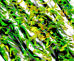
Figure 1 shows the computational domain for case M11Tw020. The simulation covers a long domain, which extends for  $L_x=315.8\delta _i$,
  $L_y=14.7\delta _i$,
  $L_z=52.7\delta _i$ in the streamwise (
 $x$), spanwise (
 $y$) and wall-normal (
 $z$) directions, where
  $\delta _i$ is the inflow boundary-layer thickness. The computations are carried out in three stages involving overlapping streamwise domains. The inflow boundary condition for Box 1 DNS is prescribed by means of a modified recycling–rescaling method (Duan et al. Reference Duan, Choudhari and Wu2014), and the recycling plane is placed at
  $52.7\delta _i$ downstream of the inflow station (i.e.
  $(x_{rec}-x_i)/\delta _i=52.7$). Time series data for primitive flow variables are saved in Boxes 1 and 2 on four spanwise wall-normal planes surrounding
  $(x-x_i)/\delta _i=78.9$ and
  $150.0$, respectively, with respect to the inflow plane of Box 1 at sampling rate
  $dt^+_{sample}=6.18\times 10^{-2}$ for a length
  $T_f u_{\tau,i}/\delta _i = 22.2$, and these time series data are provided as the inflow boundary conditions for the downstream boxes. The data are required on four planes to satisfy the boundary condition requirement of the selected WENO scheme. At run time for the Box 2 or Box 3 DNS, the saved inflow data are spline-interpolated in time to the instants dictated by the time stepping in the downstream DNS box. Numerical experiments have shown that such a procedure results in minimal disturbances to the reported turbulence statistics and coherent structures, and a similar procedure has been used widely by many other researchers for prescribing continuous inflow for DNS (Morgan et al. Reference Morgan, Duraisamy, Nguyen and Lele2013; Sillero et al. Reference Sillero, Jiménez and Moser2013).

Figure 1. Computational domain and simulation set-up for case M11Tw020.  $x = 0$ m corresponds to the leading edge of experimental flat-plate geometry of CUBRC Run 7 (Gnoffo et al. Reference Gnoffo, Berry and Van Norman2013), and the DNS domain starts downstream of the leading edge at
  $x = 0.2$ m so that it covers only the portion of the flat plate with a fully turbulent boundary layer in the experiment. The instantaneous flow is shown by the isosurface of the magnitude of the density gradient,
  $|\boldsymbol {\nabla } \rho |\delta _i/\rho _\infty \approx 0.98$ and coloured by the streamwise velocity component (with levels from 0 to
  $U_\infty$, blue to red), and the inflow boundary-layer thickness of Box 1 DNS is
  $\delta _i = 3.8$ mm.
For case M11Tw020, uniform grid spacings are used in the streamwise and spanwise directions, where the grid spacing is  $\Delta x^+=7.1$ and
  $\Delta y^+=6.6$, respectively. The grid resolutions are normalized by the viscous length
  $z_\tau$ at
  $(x-x_i)/\delta _i = 305$, which is the farthest downstream location where boundary-layer profiles are sampled for statistical analysis as listed in table 4. The grids in the wall-normal direction are clustered in the boundary layer with
  $\Delta z^+_{min}=0.43$ at the first grid point away from the wall, and the wall-normal spacing near the boundary-layer edge is kept uniform with
  $\Delta z^+_{max}=4.2$.
Details of the grid dimensions, domain size and resolutions for case M11Tw020 are listed in table 2. At the upper and outflow boundaries, unsteady non-reflecting boundary conditions based on Thompson (Reference Thompson1987) are used. The flow in the spanwise direction is assumed to be statistically homogeneous, hence periodic boundary conditions are applied in  $y$. At the wall, no-slip conditions are imposed for the three velocity components, and the wall temperature is set equal to the experimental value,
  $T_w=300$ K. The density is determined by solving the continuity equation. Additional details on the set-up of case M11Tw020 are given in Huang et al. (Reference Huang, Nicholson, Duan, Choudhari and Bowersox2020). Note that in table 2, we have defined the boundary-layer thickness
  $\delta$ as the wall-normal height where the local value of the streamwise velocity is
  $99\,\%$ of the free-stream value (
 $\bar {u}=0.99U_\infty$), consistent with that used in Zhang et al. (Reference Zhang, Duan and Choudhari2018), while the parameters reported in Huang et al. (Reference Huang, Nicholson, Duan, Choudhari and Bowersox2020) were defined based on
  $99.5\,\%$ of the free-stream value (
 $H_t=0.995H_{t,\infty }$) to facilitate comparisons with the RANS results by Gnoffo et al. (Reference Gnoffo, Berry and Van Norman2013) under the same nominal conditions as case M11Tw020.
Table 2. Summary of parameters for DNS database:  $L_x$,
  $L_y$ and
  $L_z$ are the domain size in streamwise, spanwise and wall-normal directions, respectively;
  $N_x$,
  $N_y$ and
  $N_z$ are the grid dimensions;
  $\Delta x^+$ and
  $\Delta y^+$ are the uniform grid spacings in the streamwise and spanwise directions;
  $\Delta z^+$ denotes the wall-normal spacing at the first grid away from the wall and that near the boundary-layer edge;
  $\Delta t^+$ denotes the time-step size, and
  $T_f$ is total time considered for collecting flow statistics;
  $L_{to}=U_\infty \delta _i/u_{\tau,i}$ is one turnover length of the largest eddy at inflow, where
  $\delta _i$ is the inflow boundary-layer thickness and
  $u_{\tau,i}$ the inflow friction velocity. All grid spacings are normalized by the viscous scale at the farthest downstream station selected for statistical analysis as listed in table 4.

The computational set-ups for cases M2p5HighRe and M5Tw091 parallel the set-up for the case M11Tw020 simulations, and the computational parameters for these cases are summarized in table 2. In particular, streamwise computational domains with  $L_x=313.6\delta _i$ and
  $L_x=183.6\delta _i$ are used for cases M2p5HighRe and M5Tw091, respectively, to achieve Reynolds number
  $Re_\tau \approx 1200$ in both cases. Previous DNS of spatially-developing turbulent boundary layers in the incompressible and supersonic Mach number regimes have shown that the use of very long streamwise domains is required for boundary-layer turbulence to recover from the initial transient due to inflow turbulence generation techniques and achieve a fully developed equilibrium state, which makes a highly reliable spatial simulation extremely demanding (Erm & Joubert Reference Erm and Joubert1991; Schlatter et al. Reference Schlatter, Örl’u, Li, Brethouwer, Fransson, Johansson, Alfredsson and Henningson2009; Simens et al. Reference Simens, Jiménez, Hoyas and Mizuno2009; Sillero et al. Reference Sillero, Jiménez and Moser2013; Wenzel et al. Reference Wenzel, Selent, Kloker and Rist2018). In the current study, the recovery length is characterized in terms of when the von Kármán integral equation
  $C_f = 2({\rm d}\theta /{{\rm d} x})$ is sufficiently well satisfied or by comparing results from different methods for inflow turbulence generation. Such a characterization is detailed in § 3.1. We also note that by isothermally setting the wall temperature to a prescribed constant temperature
  $T_w$ as shown in table 1, any fluctuations in the wall temperature have been suppressed, while the temperature fluctuations may not be zero over the surface of a realistic hypersonic vehicle. The previous study by Wenzel et al. (Reference Wenzel, Selent, Kloker and Rist2018) reported that allowing or suppressing wall temperature fluctuations causes no difference in turbulence statistics outside the the viscous sublayer for a Mach
  $2$ adiabatic turbulent boundary layer. However, further study may be necessary to clarify the influence of the temperature boundary condition for a hypersonic cold-wall turbulent boundary layer.
Additional information about the validation of DNS cases, including an assessment of the domain size and grid resolution as well as comparisons with available measurements from wind tunnel experiments, is given in Appendix A.
2.4. A note on averaging
In the following sections, we present the turbulence statistics that are computed by averaging first in the spanwise direction and then in the temporal direction over  $N_f$ flow-field snapshots spanning time interval
  $T_f u_\tau /\delta$. For the streamwise evolution of the peak of the Reynolds stresses discussed in § 3.2 and the skewness and flatness profiles discussed in § 4.4, the statistics are further averaged over a streamwise window (
 $[x_a-0.5\delta,x_a+0.5\delta ]$) to enhance statistical convergence, where
  $x_a$ is a reference streamwise location selected for statistical analysis (table 4). A similar technique has been used by the DNS study of Pirozzoli & Bernardini (Reference Pirozzoli and Bernardini2011). Statistical convergence is verified by calculating averages over significantly different numbers of snapshots and by making sure that the differences in flow statistics computed from different averaging intervals are negligible (
 ${<}1.3\,\%$). Throughout the paper, standard (Reynolds) averages are denoted by an overbar,
  $\bar {f}$, while density-weighted (Favre) averages are denoted by a tilde,
  $\tilde {f}=\bar {\rho f}/\bar {f}$; fluctuations around standard and Favre averages are denoted by single and double primes, as with
  $f'=f-\bar {f}$ and
  $f''=f-\tilde {f}$, respectively.
3. Spatial evolution of flow statistics
In this section, we use the DNS data to examine the spatial evolution of the various properties of the turbulent boundary layer. Together with the current DNS cases listed in table 2, the datasets for an incompressible turbulent boundary layer by Schlatter & Örlü (Reference Schlatter and Örlü2010), as well as the supersonic boundary-layer data by Pirozzoli & Bernardini (Reference Pirozzoli and Bernardini2011) and Wenzel et al. (Reference Wenzel, Selent, Kloker and Rist2018), are included as necessary to better illustrate the effects of the Mach number and wall cooling.
3.1. Characterization of inflow recovery length
In this subsection, we quantify the inflow recovery length for each DNS case, in order to allow one to infer the ‘useful’ part of the overall streamwise domain and the associated range of the Reynolds number.
In this work, the inflow recovery length is defined as  $\Delta x_{ind}=x_{ind}-x_i$, i.e. the distance from the inflow plane
  $x_i$ to the downstream location
  $x_{ind}$ where the von Kármán integral equation
  $C_f=2({\rm d}\theta /{{\rm d} x})$ is first satisfied to a specified level of accuracy. The same method was used by Wenzel et al. (Reference Wenzel, Selent, Kloker and Rist2018) in their DNS study of turbulent boundary layers with Mach numbers varying from
  $0.3$ to
  $2.5$. Consistent with Wenzel et al., we refer to the inflow recovery length based on the von Kármán integral equation as the inflow induction length. Table 3 lists the values of the inferred induction length
  $\Delta x_{ind}$ in various non-dimensional forms, and the Reynolds number range over which the boundary layer changes from the inflow profile to its equilibrium behaviour at
  $x_{ind}$. The scalings for the induction length
  $\Delta x_{ind}$ include normalization by the inflow boundary-layer thickness
  $\delta _i$, the eddy turnover length
  $L_{to}$, and the effective turnover length
  $\tilde {x}$ (Sillero et al. Reference Sillero, Jiménez and Moser2013), respectively. The eddy turnover length, defined as
  $L_{to}=U_\infty \delta _i/u_{\tau,i}$, is the advection distance of the eddies during a time interval
  $\delta _i/u_{\tau,i}$ (Simens et al. Reference Simens, Jiménez, Hoyas and Mizuno2009), where
  $u_{\tau,i}$ is the friction velocity at
  $x_i$. The effective dimensionless turnover length, first proposed by Sillero et al. (Reference Sillero, Jiménez and Moser2013) in their study of incompressible boundary layers, has the form
 \begin{equation} \tilde{x}=\int_{x_i}^{ x_{ind}}\frac{{\rm d} x}{U_\infty\delta/u_\tau}. \end{equation}
Table 3. Induction length  $\Delta x_{ind}$ in various non-dimensional forms and the corresponding variation in Reynolds numbers from the inflow plane to the end of induction length. The induction length
  $\Delta x_{ind}$ is measured as the value of
  $(x-x_i)$ where the von Kármán integral equation
  $C_f=2({\rm d}\theta /{{\rm d} x})$ is first satisfied to a specified level of accuracy of
  $5\,\%$. ‘RS’ and ‘DF’ refer to DNS cases with rescaling and digital-filtering inflow turbulence generation methods, respectively.

The induction length  $\Delta x_{ind}$ normalized by
  $\delta _i$ increases with the Mach number, with the ratio
  $\Delta x_{ind}/\delta _i$ increasing from
  $20$ at Mach
  $2.5$ to
  $80$ at Mach
  $14$. This finding is consistent with the observations by Wenzel et al. (Reference Wenzel, Selent, Kloker and Rist2018) based on data at lower Mach numbers. The induction length normalized by the eddy turnover length also increases with the Mach number and has range
  $1\lesssim \Delta x_{ind}/L_{to}\lesssim 3$. The effective dimensionless turnover length
  $\tilde {x}$ appears to better collapse the DNS data at different Mach numbers and has range
  $1\lesssim \tilde {x} \lesssim 2$.
Besides the above characterization of the induction length on the basis of  $C_f=2({\rm d}\theta /{{\rm d} x})$, the inflow recovery length is also quantified by cross-comparing data from different turbulence inflow methods. Specifically, the results based on the rescaling (RS) inflow turbulence generation are compared with those based on the digital-filtering (DF) inflow technique (Dhamankar et al. Reference Dhamankar, Martha, Situ, Aikens, Blaisdell, Lyrintzis and Li2014; Huang & Duan Reference Huang and Duan2016) for cases M2p5HighRe and M11Tw020. For this purpose, the Box 1 and Box 2 simulations of both cases were repeated with the DF inflow technique while keeping the other simulation parameters the same. Simulating the same flow with an identical set-up except for the inflow boundary condition allows a robust and reliable evaluation of the inflow recovery length.
Table 3 shows that the induction lengths for the DNS solutions based on the DF method are longer than the corresponding DNS with the RS method, and the increase in  $\Delta x_{ind}$ is equal to approximately
  $20\delta _i$ for case M2p5HighRe and
  $15\delta _i$ for case M11Tw020. The longer induction length for the DF method is also consistent with previous studies (Morgan et al. Reference Morgan, Larsson, Kawai and Lele2011; Wenzel Reference Wenzel2019). Figure 2 further compares the profiles of the van Driest (VD) transformed mean velocity and the streamwise Reynolds stress for cases M2p5HighRe and M11Tw020 at two selected streamwise locations. The upstream and downstream locations for each case approximately correspond to the end of the induction length based on the DF method and the first location selected for statistical analysis with Reynolds number
  $Re_\tau = 774$ as listed in table 4, respectively. In the near-wall region, the comparison between RS and DF methods is almost perfect for both the velocity and the streamwise Reynolds stress. There exists a small yet visible discrepancy within the wake region of the profiles between the RS and DF data at the end of the induction length
  $\Delta x_{ind}$ (
 $6.2\,\%$ for
  $u^+_{VD}$, and
  $1.8\,\%$ for
  $\overline {\rho u''u''}/\tau _w$). However, that difference has diminished downstream at
  $Re_\tau = 774$ (
 $1.5\,\%$ for
  $u^+_{VD}$, and
  $1.0\,\%$ for
  $\overline {\rho u''u''}/\tau _w$), yielding a very good comparison between the boundary-layer profiles at this second (and farther downstream) location.

Figure 2. Comparison in profiles of (a,c) the van Driest transformed velocity, and (b,d) the streamwise Reynolds stress between DNS with rescaling (RS) and digital-filtering (DF) inflow methods at the end of the induction length based on the DF method (i.e.  $x-x_i=(\varDelta _{ind})_{DF}$) and a downstream location at
  $Re_\tau = 774$. (a,b)
  $x-x_i=(\varDelta _{ind})_{DF}$; (c,d)
  $Re_\tau = 774$.
Table 4. Boundary-layer properties at the DNS station  $x_a$ selected for analysis.
  $x_i$ denotes the streamwise coordinate at the inflow plane. The boundary-layer thickness
  $\delta$ is defined as the wall-normal distance from the wall to the location where
  $\bar {u}=0.99U_{\infty }$;
  $H_{12}= \delta ^*/\theta$ is the shape factor;
  $u_\tau =\sqrt {\tau _w/\rho _w}$ is the friction velocity;
  $z_\tau =\nu _w/u_\tau$ is the viscous length;
  $B_q=q_w/(\rho _w c_p u_\tau T_w)$ is the non-dimensional surface heat flux;
  $M_\tau = u_\tau / \sqrt {\gamma R T_w}$ is the friction Mach number. Reynolds numbers are defined in table 1.

In summary, the selected DNS domains are long enough to accommodate the region that is lost to the inflow induction as well as the adjustment length. As a result, a fully developed equilibrium turbulent boundary layer that is nearly independent of the inflow effects is established in the downstream portion of the selected DNS domains for both the supersonic (Mach  $2.5$ and
  $4.9$) and hypersonic (Mach
  $11$) cases. Given the smaller recovery length for the RS method in comparison to that of the DF method, only the RS results past the inflow recovery length will be used in § 3.2 to study the spatial evolution of wall and turbulence properties and to derive Reynolds number scaling for equilibrium boundary layers in the high-speed regime.
3.2. Spatial evolution of mean and turbulence properties
The van Driest II transformation (Van Driest Reference Van Driest1956) and the Spalding & Chi transformation (Spalding & Chi Reference Spalding and Chi1964) are two of the most commonly used models to estimate the skin friction associated with a compressible boundary layer in terms of an equivalent, incompressible boundary layer. For both van Driest II and Spalding & Chi theories, the transformation can be represented by
 \begin{gather} C_{f,i}=F_c\,C_f, \end{gather}
 \begin{gather}Re_{\theta,i}=F_\theta\,Re_\theta, \end{gather}
where  $C_{f,i}$ and
  $Re_{\theta,i}$ are the equivalent (i.e. transformed) ‘incompressible’ skin friction coefficient and momentum thickness Reynolds number, respectively, and
  $F_c$ and
  $F_\theta$ are transformation factors that depend on flow parameters such as the Mach number, free-stream static and wall temperatures, and recovery factor. The transformation factor
  $F_c$ is the same in both van Driest II and Spalding & Chi theories, and can be written as (Rumsey Reference Rumsey2010)
 \begin{equation} F_c = \frac{T_r/T_\infty-1}{\left(\sin^{{-}1}A+\sin^{{-}1}B\right)^2}, \end{equation}
where  $A$ and
  $B$ are given as
 \begin{equation} \left.\begin{gathered} A = \frac{2a^2-b}{\left(b^2+4a^2\right)^{1/2}},\quad B = \frac{b}{\left(b^2+4a^2\right)^{1/2}}\\ a=\left(r\,\frac{\gamma-1}{2}\,M^2_\infty\,\frac{T_\infty}{T_w}\right)^{1/2},\quad b = \frac{T_r}{T_w}-1. \end{gathered}\right\} \end{equation}
However, the other transformation factor,  $F_{\theta }$, is different between the two theories and is given as
 \begin{equation} (F_{\theta})_{VD}=\mu_\infty/\mu_w, \quad (F_{\theta})_{SC}=(T_\infty/T_w)^{{-}0.702}(T_r/T_w)^{{-}0.772}, \end{equation}
where the subscripts ‘VD’ and ‘SC’ refer to the transformation factors from the van Driest II and Spalding & Chi theories, respectively. After (3.2) and (3.3) are applied to compressible data to obtain the equivalent incompressible values of  $C_{f,i}$ and
  $Re_{\theta,i}$, these transformed values can be compared to the friction correlations developed for incompressible flows. Three commonly used incompressible friction correlations are the Kármán–Schoenherr relation (Roy & Blottner Reference Roy and Blottner2006), the power-law correlation by Smits, Matheson & Joubert (Reference Smits, Matheson and Joubert1983), and the modified Coles–Fernholz relation (Nagib, Chauhan & Monkewitz Reference Nagib, Chauhan and Monkewitz2007):
 \begin{gather} \rm{K\unicode{x00E1}rm\unicode{x00E1}n-Schoenherr:} \quad (C_{f,i})_{KS} =\left(\log_{10}(2Re_{\theta i})[17.075\log_{10}(2Re_{\theta i})+14.832]\right)^{{-}1} , \end{gather}
 \begin{gather}\text{Smits}\, {et al}.\text{:}\quad (C_{f,i})_{SM}=0.024\,Re_{\theta i}^{{-}1/4} , \end{gather}
 \begin{gather}\text{Coles-Fernholz:}\quad (C_{f,i})_{CF} =2[2.604\log{Re_{\theta i}}+4.127]^{{-}2}. \end{gather}
 Although multiple previous studies compared the performance of these two theories for hypersonic cold-wall turbulent boundary layers, they had drawn different conclusions as to which theory to recommend. Specifically, Hopkins & Inouye (Reference Hopkins and Inouye1971) compared the van Driest II and Spalding & Chi transformation theories on skin friction measurements at  $M_\infty = 2.8-7.4$ and
  $T_w/T_r = 0.14-1.0$, and they concluded that the van Driest II theory performed better. Holden (Reference Holden1972) performed skin friction measurement in a shock tunnel with
  $M_\infty = 7-13$ and
  $0.14\leqslant h_w/h_{aw} \leqslant 0.3$; he concluded that the theory of Spalding & Chi was in best agreement with the experimental measurements in the Mach number range 7–10, while the van Driest II transformation was a better predictor of the skin friction levels at Mach numbers between 10 and 13. The review by Bradshaw (Reference Bradshaw1977) endorsed Hopkins & Inouye's choice of the van Driest II theory but also commented that the theory failed to predict the skin friction on a very cold wall (
 $T_w/T_r\leqslant 0.1-0.2$). In a more recent study, Goyne, Stalker & Paull (Reference Goyne, Stalker and Paull2003) found that the Spalding & Chi method was the most suitable theory for high-enthalpy hypersonic boundary-layer flows in an equilibrium turbulent state, based on their skin friction measurements in a free-piston shock tunnel with air-flow Mach number
  $4.4\leqslant M_\infty \leqslant 6.7$ and wall-to-stagnation enthalpy ratio
  $0.02\leqslant h_w/h_{aw} \leqslant 0.1$. Here, the DNS data will be used to extend the comparison between the two transformation theories to a broader range of Mach number and wall-to-recovery temperature ratio and, also, to provide an independent assessment related to an optimal choice for the incompressible correlation.
Figure 3 compares the performance of van Driest II and Spalding & Chi transformations for the current DNS cases. The skin friction values based on both the van Driest II and Spalding & Chi transformations are in good agreement with the incompressible correlations for the Mach 2.5, adiabatic wall case (M2p5HighRe). The performance of the van Driest II transformation remains good for the hypersonic cases corresponding to a moderately cold wall ( $0.3 \lesssim T_w/T_r < 1.0$). However, for the hypersonic cases M11Tw020 and M14Tw018 that correspond to a highly cooled wall (
 $T_w/T_r \lesssim 0.3$), neither of the two theories can provide a good prediction. The van Driest II transformation tends to overpredict
  $C_f$ by up to 10–20 % and the Spalding & Chi theory underpredicts
  $C_f$ by 20–40 %. Such a trend is consistent with the findings of Hopkins & Inouye (Reference Hopkins and Inouye1971). It is also interesting to note that the discrepancy between the Spalding & Chi transformed skin friction values for the hypersonic cold-wall case M11Tw020 and the incompressible correlations decreases gradually at increasing Reynolds numbers. This improvement in the model accuracy at high Reynolds numbers is consistent with the measurements of Goyne et al. (Reference Goyne, Stalker and Paull2003), who found that the Spalding & Chi method best predicted the skin friction coefficient in cold-wall, high-Mach-number and high-enthalpy flows, provided that the boundary layer has a sufficient fetch downstream of the transition region to allow the boundary-layer turbulence to relax from the transitional to the fully turbulent state. Among the various combinations of compressible transformations and incompressible correlations for the skin friction, the combination of van Driest II transformation with the power-law relation of Smits et al. (Reference Smits, Matheson and Joubert1983) correlates best with the DNS data, at least for the Reynolds number range covered by the current DNS. Such a combination predicts the skin friction within
  ${\pm }5\,\%$ for the supersonic adiabatic-wall case, and within
  $-15\%$ to
  $-6\,\%$ for the hypersonic cold-wall cases (figure 3c).

Figure 3. Transformed skin friction coefficient ( $C_{f,i}=F_c C_f$) versus Reynolds numbers (
 $Re_{\theta,i}=F_\theta \,Re_{\theta }$) based on (a) the van Driest II theory and (b) the Spalding & Chi theory, wherein the black solid line, the dashed line and the dash-dotted line denote the incompressible correlations of Kármán–Schoenherr (Roy & Blottner Reference Roy and Blottner2006), Smits et al. (Reference Smits, Matheson and Joubert1983) and Coles–Fernholz (Nagib et al. Reference Nagib, Chauhan and Monkewitz2007), respectively. The relative difference between the DNS and the theoretical prediction based on a combination of van Driest II transformation with the power-law relation of Smits et al. (Reference Smits, Matheson and Joubert1983) (i.e.
  $C_{f,the}=(C_{f,i})_{SM}/(F_{c})_{VD}$) is shown in (c).
With a known skin friction coefficient, the Reynolds analogy factor  $R_{af}=2C_h/C_f$ is often used to predict the surface heat flux (Roy & Blottner Reference Roy and Blottner2006). Here,
  $C_h=q_w/(\rho _\infty U_\infty c_p(T_r-T_w))$ is the Stanton number, and
  $C_f=2\tau _w/(\rho _\infty U_\infty ^2)$ is the skin friction coefficient. Figure 4(a) shows the distribution of
  $R_{af}$ as a function of the friction Reynolds number
  $Re_\tau$. Over the Reynolds number range covered by the current DNS, the Reynolds analogy factor
  $R_{af}$ is nearly constant for all hypersonic cold-wall cases, with its value bracketed within the narrow range
  $1.1< R_{af}<1.2$, consistent with the usual approximation
  $R_{af}=Pr^{-2/3} \approx 1.256$. For case M11Tw020, in particular, the Reynolds analogy factor
  $R_{af}$ is approximately
  $1.19$ for
  $Re_\tau \lesssim 400$, and gradually decreases to
  $1.16$ as the Reynolds number is increased to
  $Re_\tau \approx 1172$. The latter value (
 $R_{af} = 1.16$) was also recommended by Chi & Spalding (Reference Chi and Spalding1966) and Hopkins & Inouye (Reference Hopkins and Inouye1971). Figures 4(b) and 4(c) further compare
  $R_{af}=2C_h/C_f$ against the experimental measurements of Goyne et al. (Reference Goyne, Stalker and Paull2003) and Holden (Reference Holden1972). The values of the Reynolds analogy factor based on the DNS fall within the scatter of the experimental measurements at similar unit Reynolds numbers
  $Re_u$ and enthalpy ratios
  $h_w/h_0$. However, the variation in
  $R_{af}$ across the various DNS cases is significantly smaller than that in the experiments.

Figure 4. The Reynolds analogy factor  $R_{af}=2C_h/C_f$ as a function of (a) friction Reynolds number
  $Re_\tau$, (b) unit Reynolds number
  $Re_u=\rho _\infty U_\infty /\mu _\infty$, and (c) wall-to-total enthalpy ratio
  $h_w/h_0$. Solid triangle symbol denotes experimental measurement by Goyne et al. (Reference Goyne, Stalker and Paull2003), and circle symbol by Holden (Reference Holden1972). The horizontal solid, dashed and dotted lines denote constant values of unity,
  $1.16$ and
  $Pr^{-2/3}$, with
  $Pr= 0.71$, respectively.
Figure 5(a) plots the shape factor  $H_{12}= \delta ^*/\theta$ as a function of the friction Reynolds number
  $Re_\tau$. The shape factor
  $H_{12}$ is observed to be insensitive to the Reynolds number, but it varies significantly with Mach number and wall temperature conditions, ranging from
  $H_{12} \approx 4$ for case M2p5 to
  $H_{12} \approx 54$ for case M14Tw018. Figure 5(b) shows
  $H_{12}$ as a function of the free-stream Mach number
  $M_\infty$, and its comparison with the empirical relations of Hopkins et al. (Reference Hopkins, Keener, Polek and Dwyer1972), Shahab et al. (Reference Shahab, Lehnasch, Gatski and Comte2011), and Wood (Reference Wood1964). The three empirical relations are given as follows:
 \begin{gather} \text{Hopkins }\textit{et al.:}\quad H_{12,the}=\frac{4(1+0.344M_\infty^2)}{3\left(2-\dfrac{T_w}{T_r}\right)^{1.35}}, \end{gather}
 \begin{gather}\text{Shahab} \,{et al}.\text{:}\quad H_{12,the}=1.4+0.4M_\infty^2-1.222\,\frac{T_r}{T_\infty}\left(1-\frac{T_w}{T_r}\right), \end{gather}
 \begin{gather}\text{Wood:}\quad H_{12,the}=1.222+0.4M_\infty^2-1.222\,\frac{T_r}{T_\infty}\left(1-\frac{T_w}{T_r}\right). \end{gather}
Consistent with the above theories, the DNS-predicted  $H_{12}$ increases dramatically with Mach number, while wall cooling significantly decreases
  $H_{12}$ with respect to the reference adiabatic value at each Mach number. Among the three empirical shape-factor relations, the relation by Hopkins et al. (Reference Hopkins, Keener, Polek and Dwyer1972) provides the best correlation with the DNS data, with a relative error of approximately
  $2\,\%$ for the supersonic adiabatic case, and up to
  $8\,\%$ for the hypersonic cold-wall cases (figure 5c).

Figure 5. Shape factor  $H_{12}= \delta ^*/\theta$ as a function of (a) friction Reynolds number
  $Re_\tau$, and (b,c) free-stream Mach number
  $M_\infty$. In (b), lines denote the reference adiabatic shape factor value predicted by (3.8) with
  $T_w/T_r = 1.0$. Dash-dotted line, Hopkins et al. (Reference Hopkins, Keener, Polek and Dwyer1972); dashed line, Shahab et al. (Reference Shahab, Lehnasch, Gatski and Comte2011); solid line, Wood (Reference Wood1964).
In addition to mean wall and integral parameters, the streamwise development of the fluctuation statistics are investigated by using the DNS data, including the near-wall peak values of the Reynolds stresses and the fluctuating wall quantities. Figure 6 shows the magnitude of the near-wall peak of the streamwise Reynolds stress in the semilocal scaling ( $(u''_{rms})^*=(\overline {\rho u''u''}/\tau _w)^{1/2}$) as functions of
  $Re_\tau$ and
  $Re_\tau ^*$. Reference data including the Mach
  $2$ data of Pirozzoli & Bernardini (Reference Pirozzoli and Bernardini2011) and the incompressible data of Sillero et al. (Reference Sillero, Jiménez and Moser2013) and Lee & Moser (Reference Lee and Moser2015) are also plotted for comparison. At Mach
  $2.5$, the peak magnitude
  $(u''_{rms})^*_{pk}$ compares well with reference data and shows a weak increase with both Reynolds numbers, and the dependence of
  $(u''_{rms})^*_{pk}$ with the Reynolds number follows the logarithmic fits (Pirozzoli & Bernardini Reference Pirozzoli and Bernardini2013; Lee & Moser Reference Lee and Moser2015)
 \begin{equation} (u'')^*_{pk}=\sqrt{3.352+0.725\log Re_\tau}, \quad (u'')^*_{pk}=\sqrt{3.66+0.642\log Re_\tau^*}. \end{equation}
However,  $(u''_{rms})^*_{pk}$ for the hypersonic cold-wall cases remains nearly constant throughout the Reynolds number range covered by the DNS data. The semilocal scaling largely accounts for the influence of wall temperature on the near-wall peak magnitude, as seen by the collapse of
  $(u''_{rms})^*_{pk}$ between the cases M6Tw025 and M6Tw076. However, the peak value of the scaled streamwise Reynolds stress indicates a weak increase with the free-stream Mach number. At
  $Re_\tau = 1138$, for instance,
  $(u''_{rms})^*_{pk}$ increases from
  $2.9$ for case M2p5HighRe to
  $3.5$ for case M11Tw020. The increase in
  $(u''_{rms})^*_{pk}$ with the Mach number is consistent with the previous studies of turbulent channel and boundary-layer flows (Modesti & Pirozzoli Reference Modesti and Pirozzoli2016; Zhang et al. Reference Zhang, Duan and Choudhari2018; Yao & Hussain Reference Yao and Hussain2020).

Figure 6. Peak magnitude of the normalized streamwise Reynolds stress  $(u'')^*=(\overline {\rho u''u''}/\tau _w)^{1/2}$ as a function of (a)
  $Re_\tau$, and (b)
  $Re_\tau ^*$. Solid symbols: circles, Pirozzoli & Bernardini (Reference Pirozzoli and Bernardini2011) at
  $M_\infty =2$; triangle, Sillero et al. (Reference Sillero, Jiménez and Moser2013) at
  $M_\infty \approx 0$; diamond, Lee & Moser (Reference Lee and Moser2015) at
  $M_\infty \approx 0$. Black solid line denotes
  $(u'')^*_{pk}=\sqrt {3.352+0.725\log Re_\tau }$ (Pirozzoli & Bernardini Reference Pirozzoli and Bernardini2013) in (a), and
  $(u'')^*_{pk}=\sqrt {3.66+0.642\log Re_\tau ^*}$ (Lee & Moser Reference Lee and Moser2015) in (b).
Figure 7 further shows the magnitude of the near-wall peak of the Reynolds shear stress in the semilocal scaling ( $(u''w'')^*=-\overline {\rho u''w''}/\tau _w$) as functions of
  $Re_\tau$ and
  $Re_\tau ^*$. Similar to the streamwise Reynolds stress
  $(u''_{rms})^*$, the magnitude of
  $(u''w'')^*$ shows a weak increase with Reynolds number and follows the scaling relation
 \begin{equation} (u''w'')^*_{pk}=1-8.5\,Re_\tau^{*-2/3} \end{equation}
for  $Re_\tau ^*\lessapprox 2000$, and the relation
 \begin{equation} (u''w'')^*_{pk}=1-3.0\,Re_\tau^{*-1/2} \end{equation}
for higher  $Re_\tau ^*$ (Yao & Hussain Reference Yao and Hussain2020).

Figure 7. Peak magnitude of the normalized Reynolds shear stress  $(u''w'')^*=-\overline {\rho u''w''}/\tau _w$ as a function of (a)
  $Re_\tau$, and (b)
  $Re_\tau ^*$. In (b), the solid line denotes
  $(u''w'')^*_{pk}=1-8.5\,Re_\tau ^{*-2/3}$, and the dashed line denotes
  $(u''w'')^*_{pk}=1-3.0\,Re_\tau ^{*-1/2}$.
Figure 8 shows the distribution of the normalized intensity of wall pressure fluctuations as a function of the Reynolds number. The intensity of wall pressure fluctuations normalized by the mean wall pressure (figure 8a) decreases with Reynolds number and increases with Mach number and the wall temperature ratio. For instance,  $p'_{w,rms}/\bar {p}_w$ increases from approximately
  $4\,\%$ at Mach
  $2.5$ to
  $25\,\%$ at nominally Mach
  $11$. The intensity of wall pressure fluctuations becomes less sensitive to the flow parameters when normalized by the local wall shear stress
  $\tau _w$ (figure 8b), consistent with multiple previous findings (Pirozzoli & Bernardini Reference Pirozzoli and Bernardini2011; Duan et al. Reference Duan, Choudhari and Wu2014, Reference Duan, Choudhari and Zhang2016; Zhang et al. Reference Zhang, Duan and Choudhari2017). For adiabatic or nearly adiabatic cases (
 $T_w/T_r= 0.7-1.0$),
  $p'_{w,rms}/\tau _w$ shows a weak logarithmic increase with the friction Reynolds number as (Pirozzoli & Bernardini Reference Pirozzoli and Bernardini2011)
 \begin{equation} p'_{w,rms}/\tau_w=\sqrt{6.5+1.86\log_{10}(\max(Re_\tau/333,1))}, \end{equation}
and the DNS values of the normalized pressure fluctuations fall within the narrow range 2.6–2.8. This range is also in agreement with the adiabatic results of Pirozzoli & Bernardini (Reference Pirozzoli and Bernardini2011) at  $M_\infty = 2 - 4$. For cold-wall cases (
 $T_w/T_r < 0.5$), however,
  $p'_{w,rms}/\tau _w$ is almost a constant in the Reynolds number range covered by the current DNS. For cases M6Tw025 and M8Tw048, we found that
  $p'_{w,rms}/\tau _w \approx 3.6$ , whereas and
  $p'_{w,rms}/\tau _w \approx 4.5$ at Mach 11 and 14. Figure 8(c) further shows the wall pressure fluctuation normalized in mixed scaling,
  $p'_{w,rms}/(\rho _w u_\tau U_\infty )$, which has been found to yield the best collapse of the wall pressure fluctuations in incompressible boundary layers over a wide range of Reynolds numbers (Schlatter et al. Reference Schlatter, Örl’u, Li, Brethouwer, Fransson, Johansson, Alfredsson and Henningson2009, Reference Schlatter, Li, Brethouwer, Johansson and Henningson2010; Tsuji et al. Reference Tsuji, Fransson, Alfredsson and Johansson2007). For the supersonic and hypersonic cases simulated in the present work, the value of
  $p'_{w,rms}/(\rho _w u_\tau U_\infty )$ varies between
  $0.12$ and
  $0.17$, and this range is narrower than the corresponding variations in
  $p'_{w,rms}/\overline {p}_w$ and
  $p'_{w,rms}/\tau _w$. The compressible values of
  $p'_{w,rms}/(\rho _w u_\tau U_\infty )$ are larger than the typical incompressible value of
  $0.112$, as reported by Schlatter et al. (Reference Schlatter, Örl’u, Li, Brethouwer, Fransson, Johansson, Alfredsson and Henningson2009, Reference Schlatter, Li, Brethouwer, Johansson and Henningson2010).

Figure 8. Intensity of wall pressure fluctuation as a function of Reynolds number, normalized by (a) wall mean pressure  $p'_{w,rms}/p_w$, (b) wall shear stress
  $p'_{w,rms}/\tau _w$, and (c) mixed scale
  $p'_{w,rms}/(\rho _w u_\tau U_\infty )$. In (b), the black solid line denotes
  $p'_{w,rms}/\tau _w=\sqrt {6.5+1.86\log _{10}(\max (Re_\tau /333,1))}$ (Pirozzoli & Bernardini Reference Pirozzoli and Bernardini2011), and the triangular and diamond solid symbols represent supersonic adiabatic and incompressible DNS data by Bernardini & Pirozzoli (Reference Bernardini and Pirozzoli2011b) and Schlatter et al. (Reference Schlatter, Örl’u, Li, Brethouwer, Fransson, Johansson, Alfredsson and Henningson2009), respectively. The dashed horizontal line in (c) corresponds to a typical incompressible value of
  $0.112$ as reported by Schlatter et al. (Reference Schlatter, Örl’u, Li, Brethouwer, Fransson, Johansson, Alfredsson and Henningson2009, Reference Schlatter, Li, Brethouwer, Johansson and Henningson2010).
Figure 9 displays the root-mean-square (r.m.s.) fluctuations in wall shear stress and surface heat flux as functions of the friction Reynolds number  $Re_\tau$. In both cases, the fluctuation amplitudes account for an even larger fraction of the respective mean values, in comparison with the wall pressure fluctuation
  $p'_{w,rms}/p_w$ as shown in figure 8(a). At Mach
  $2.5$,
  $\tau '_{w,rms}/\tau _w$ is approximately
  $0.4$ at low Reynolds numbers (
 $Re_\tau \lesssim 400$);
  $\tau '_{w,rms}/\tau _w$ for adiabatic or nearly adiabatic cases (
 $T_w/T_r= 0.7-1.0$) increases slowly with the Reynolds number and matches the incompressible fit of Schlatter & Örlü (Reference Schlatter and Örlü2010),
 \begin{equation} \tau'_{w,rms}/\tau_w=0.298+0.018\log{Re_\tau}. \end{equation}
For hypersonic cold-wall cases,  $\tau '_{w,rms}/\tau _w$ and
  $q'_{w,rms}/q_w$ show a small decrease with increasing Reynolds number, with
  $\tau _{w,rms}/\tau _w \simeq 0.45 - 0.5$ and
  $q_{w,rms}/q_w \simeq 0.5 - 0.7$ among various Mach number and wall temperature conditions and the Reynolds number range covered by the current DNS.

Figure 9. (a) The r.m.s. wall shear stress fluctuation  $\tau '_{w,rms}/\tau _w$, and (b) the r.m.s. wall heat flux fluctuation
  $q'_{w,rms}/\bar {q}_w$ as a function of the friction Reynolds number
  $Re_\tau$. In (a), the solid black symbols represent the incompressible DNS data of Schlatter & Örlü (Reference Schlatter and Örlü2010), and the black solid line denotes the incompressible fit of
  $\tau '_{w,rms}/\tau _w=0.298+0.018\log {Re_\tau }$ (Schlatter & Örlü Reference Schlatter and Örlü2010).
4. Local turbulence statistics
In this section, boundary-layer profiles are extracted at selected streamwise locations from various DNS cases, and the local turbulence statistics at each location are presented. The results are used to assess various compressibility scaling relations at higher Reynolds numbers as well as to study Reynolds number effects on turbulence statistics in the high-Mach-number cold-wall regime. Table 4 lists the values of the mean boundary-layer parameters at the locations selected for the statistical analysis. For each DNS case, boundary-layer profiles at two selected streamwise locations, both of which are downstream of the initial adjustment zone, are used to gauge the effects of the streamwise evolution (or, alternatively, the effects of the local Reynolds number) on the boundary-layer statistics.
4.1. Mean velocity profile
The van Driest transformation (Van Driest Reference Van Driest1951) is commonly used to transform the mean velocity profile in a compressible boundary layer to an equivalent profile from an incompressible boundary layer by accounting for the mean property variations across the thickness of the boundary layer:
 \begin{equation} u^+_{VD} = \int_0^{\bar{u}^+}(\bar{\rho}/\bar{\rho}_w)^{1/2}\,{\rm d}\bar{u}^+. \end{equation}
Although the classic van Driest transformation is able to collapse the compressible velocity profile to the incompressible law of wall for supersonic boundary layers with an adiabatic wall, its performance was found to deteriorate under hypersonic cold-wall conditions (Duan et al. Reference Duan, Beekman and Martin2010; Zhang et al. Reference Zhang, Duan and Choudhari2018). Recently, Trettel & Larsson (Reference Trettel and Larsson2016) proposed a new transformation based on the log-law and stress-balance conditions
 \begin{gather} u^+_{TL} = \int_0^{u^+}\left(\frac{\bar{\rho}}{\rho_w} \right)^{1/2}\left[1+ \frac{1}{2}\,\frac{1}{\bar{\rho}}\,\frac{{\rm d}\bar{\rho}}{{\rm d}z}\,z-\frac{1}{\bar{\mu}}\, \frac{{\rm d}\bar{\mu}}{{\rm d}z}\,z \right]{\rm d}u^+ , \end{gather}
 \begin{gather}z^* = \frac{\bar{\rho}(\tau_w/\bar{\rho})^{1/2}z}{\bar{\mu}}. \end{gather}
While the Trettel & Larsson transformation was quite successful in collapsing the viscous sublayer and buffer layer of a velocity profile from a non-adiabatic turbulent boundary layer to an equivalent incompressible profile, there is still substantial disagreement in the log-law region of the velocity profile (Wu et al. Reference Wu, Bi, Hussain and She2017; Zhang et al. Reference Zhang, Duan and Choudhari2018). To improve the overall collapse of the mean velocity profile for the boundary-layer cases, Volpiani et al. (Reference Volpiani, Iyer, Pirozzoli and Larsson2020) proposed a data-driven approach that uses data fitting to determine the non-dimensionalizations for wall disturbance and velocity
 \begin{gather} u^+_{V} = \int_0^{u^+} \frac{(\bar{\rho}/\bar{\rho}_w)^{1/2}}{(\bar{\mu}/\bar{\mu}_w)^{1/2}}\,{\rm d}u^+ , \end{gather}
 \begin{gather}z^+_{V} = \int_0^{z^+} \frac{(\bar{\rho}/\bar{\rho}_w)^{1/2}}{(\bar{\mu}/\bar{\mu}_w)^{3/2}}\,{\rm d}z^+. \end{gather}
They showed that the data-driven transformation led to an improved overall collapse of the mean velocity profile for hypersonic cold-wall boundary layers when compared to that of Trettel & Larsson (Reference Trettel and Larsson2016). Griffin, Fu & Moin (Reference Griffin, Fu and Moin2021) further proposed a velocity transformation for compressible wall-bounded turbulent flows by accounting for distinct effects of compressibility on the viscous stress and turbulent shear stress. Their method is referred to as the total-stress-based transformation and has the form
 \begin{equation} u^+_{TS} = \int_0^{u^+} \frac{S_{eq}^+}{1+S_{eq}^+{-}S_{TL}^+}\,{\rm d}z^*, \end{equation}
where  $S_{eq}^+=(\bar {\mu }_w/\bar {\mu })(\partial u^+/\partial z^*)$ and
  $S_{TL}^+=(\bar {\mu }/\bar {\mu }_w)(\partial u^+/\partial z^+)$. By scaling the viscous stress with the semilocal non-dimensionalization in the viscous sublayer and treating the Reynolds shear stress to maintain the approximate equilibrium of turbulence production and dissipation in the log-law region, the total-stress-based transformation was found to successfully collapse the velocity profile for a wide range of flows, including heated, cooled and adiabatic boundary layers, and fully developed channel and pipe flows.
All the previous studies on mean velocity transformations for hypersonic turbulent boundary layers were limited to low Reynolds numbers ( $Re_\tau \lesssim 600$), therefore their performance at higher Reynolds numbers is largely unknown. Here, we will provide a more systematic study of velocity transformations by using the latest DNS database, in an attempt to shed further light on the effect of Reynolds number on the efficacy of these compressibility transformations.
Figure 10(a) plots the van Driest transformed mean streamwise velocity profiles at two different Reynolds numbers for each DNS case. At each of these Mach numbers, the van Driest transformed velocity profile includes an approximately logarithmic region, wherein  $u_{VD}^+ = (1/k) \log (z^+) + C_{VD}$, and the extent of this logarithmic region increases with the Reynolds number. Compared to the quasiadiabatic cases at Mach
  $2.5$ and
  $4.9$, the transformed velocity for the hypersonic cold-wall case shows an apparent decrease in the mean slope within the linear and viscous sublayer and an increase in the log-layer intercept
  $C_{VD}$. Such a trend is consistent with the previous studies of hypersonic turbulent boundary layers at lower Reynolds numbers (Duan et al. Reference Duan, Beekman and Martin2011; Zhang et al. Reference Zhang, Duan and Choudhari2018). Under the Trettel and Larsson transformation, the velocity profiles
  $u_{TL}^+$ at different Mach numbers and wall cooling rates collapse in the viscous sublayer and buffer layer (figure 10b). However, an apparent difference is still seen in the log-layer intercept
  $C_{TL}$ between the two different flow conditions. Although not shown in the figure, a scatter of
  $u_{TL}^+$ similar to that of the van Driest transformed velocity
  $u^+_{VD}$ remains even at a common semilocal Reynolds number
  $Re^*_\tau = \rho_\delta \sqrt{\tau_w/\rho_\delta} \delta/\mu_\delta$. We also noted that the significant scatter among the log-law intercept
  $C_{TL}$ values for the different Mach number and wall temperature cases was not observed for compressible channel flows, where the Trettel and Larsson transformation was found to yield a nearly perfect collapse among the isothermally cold-wall velocity profiles (Trettel & Larsson Reference Trettel and Larsson2016; Yao & Hussain Reference Yao and Hussain2020). The difference in the behaviour of the log-law intercept between boundary layers and channel flows may suggest a stronger influence of the cooling parameter on the balance between turbulent and viscous shear stresses in the case of external boundary layers.

Figure 10. Effect of applying, to the mean velocity profile, (a) the van Driest (VD) transformation ( $U_{VD}^+$), (b) the Trettel and Larsson (TL) transformation (
 $U_{TL}^+$), (c) the data-driven-based transformation of Volpiani et al. (Reference Volpiani, Iyer, Pirozzoli and Larsson2020) (
 $U_V^+$), and (d) the total-stress-based transformation of Griffin et al. (Reference Griffin, Fu and Moin2021) (
 $U_{TS}^+$).
An assessment of the data-driven-based transformation of Volpiani et al. (Reference Volpiani, Iyer, Pirozzoli and Larsson2020) is shown in figure 10(c) for various DNS cases. The transformed mean velocity profiles at different Mach numbers and wall cooling rates successfully collapse to the incompressible law of the wall both in the viscous sublayer and in the log-layer regions, consistent with the findings of Volpiani et al. (Reference Volpiani, Iyer, Pirozzoli and Larsson2020) at lower Reynolds numbers. Such a good performance is not unexpected as the data-driven method of Volpiani et al. (Reference Volpiani, Iyer, Pirozzoli and Larsson2020) was developed using non-adiabatic boundary-layer cases in their training database. Figure 10(d) further shows the total-stress-based transformed mean velocity profiles for current DNS data. A similarly good agreement is achieved among various DNS data. Given that the total-stress-based transformation of Griffin et al. (Reference Griffin, Fu and Moin2021) was developed by scaling separately the viscous stress with the semilocal non-dimensionalization and the Reynolds shear stress with the assumption of turbulence quasi-equilibrium (i.e. approximate equilibrium of turbulence production and dissipation), the good collapse of the total-stress-based transformed velocity profiles suggests that a physics-based mapping between the compressible and incompressible mean velocity profiles of wall-bounded turbulent flows must account for distinct effects of compressibility on the viscous stress and turbulent shear stress.
To quantify further the extent of the region with a logarithmic velocity variation, a log-law diagnostic function similar to that of Pirozzoli & Bernardini (Reference Pirozzoli and Bernardini2013) is introduced:
 \begin{equation} I_c = \hat{Z}({\rm d} u_c^+{/}{\rm d} \hat{Z}), \end{equation}
where  $u_c^+$ and
  $\hat {Z}$ are the transformed mean velocity and non-dimensional wall disturbance, respectively, for various compressibility transformations. Based on the above definition, a constant value of the diagnostic function
  $I_c$ would imply a perfectly logarithmic behaviour. Figure 11 shows that the diagnostic function for the van Driest transformed velocity,
  $I_{VD}$, is nearly constant over the range
  $z^+ \approx 40 - 100$ for the two supersonic cases M2p5HighRe and M5Tw091 at
  $Re_\tau = 1172$ (i.e.
  $Re_\tau ^* = 2626$ for M2p5HighRe, and
  $Re_\tau ^*=9178$ for M5Tw091). On the other hand, the hypersonic cold-wall case M11Tw020 does not display a significantly wide region of constant diagnostic function
  $I_{VD}$ for Reynolds numbers up to
  $Re_\tau = 1172$ (
 $Re_\tau ^* = 6213$). The lack of constancy in the diagnostic function for case M11Tw020 may suggest the absence of a wall-normal region with a strictly logarithmic behaviour for the hypersonic cold-wall case. The strong wall cooling in this case tends to reduce the scale separation between the large and small turbulence scales, preventing the velocity profile from forming a visible log-law region, even at Reynolds numbers as high as
  $Re_\tau = 1172$ (
 $Re_\tau ^* = 6213$). The diagnostic function for the other three transformations shows existence and absence of constancy similar to that of the van Driest transformation for the supersonic and hypersonic cases, respectively. A comparison in
  $I_c$ at
  $\hat {Z}\lesssim 100$ among the various diagnostic functions further suggests that the total-stress based transformation provides the best collapse of the DNS data across the inner layer of the boundary layer (including the viscous sublayer, buffer layer and logarithmic layer).

Figure 11. The diagnostic function  $I_c = \hat {Z}({\rm d} u_c^+/{\rm d} \hat {Z})$ of transformed velocities for cases M2p5HighRe, M5Tw091 and M11Tw020, with (a)
  $u_c^+ = u_{VD}^+$ and
  $\hat {Z} = z^+$ for van Driest (VD) transformation, (b)
  $u_c^+ = u_{TL}^+$ and
  $\hat {Z} = z^*$ for Trettel and Larsson (TL) transformation, (c)
  $u_c^+=u_{V}^+$ and
  $\hat {Z} = z_V^+$ for the data-driven-based transformation of Volpiani et al. (Reference Volpiani, Iyer, Pirozzoli and Larsson2020) (V), and (d)
  $u_c^+=u_{TS}^+$ and
  $\hat {Z} = z^*$ for the total-stress-based (TS) transformation of Griffin et al. (Reference Griffin, Fu and Moin2021). The solid red square symbol in (a) indicates DNS data (
 $Re_\tau \approx 1113$) by Pirozzoli & Bernardini (Reference Pirozzoli and Bernardini2013), and the solid black circle symbol from DNS data (
 $Re_\tau \approx 5200$) by Lee & Moser (Reference Lee and Moser2015). The black dashed line represents the general shape of the composite profile by Monkewitz, Chauhan & Nagib (Reference Monkewitz, Chauhan and Nagib2007).
The turbulent velocity profile may also be represented by a power law of the form (Johnson & Bushnell Reference Johnson and Bushnell1970)
 \begin{equation} \frac{\bar{u}}{U_\infty}=\left(\frac{z}{\delta_\infty}\right)^{1/N}, \end{equation}
where  $\delta _\infty$ is the thickness where the streamwise velocity first reaches the free-stream velocity
  $U_\infty$. A quantitative verification of the power-law behaviour can be obtained by plotting the power-law diagnostic function defined as
 \begin{equation} N=\left(\frac{z}{\bar{u}}\,\frac{\partial \bar{u}}{\partial z}\right)^{{-}1}, \end{equation}
whose constancy would imply a perfect power-law behaviour. Figure 12(a) plots the power-law diagnostic function as a function of the wall-normal distance for cases M2p5HighRe, M5Tw091 and M11Tw020. The diagnostic function for the mean streamwise velocity  $\bar {u}$ nearly plateaus in the region
  $0.2 \lesssim z/\delta \lesssim 0.6$, and the power-law exponent
  $N$ varies between
  $5$ and
  $8$ among the different DNS cases. A similar diagnostic function for the van Driest transformed streamwise velocity can be defined to gauge the power-law behaviour of
  $\bar {u}_{VD}$. Figure 12(b) shows that the van Driest transformed streamwise velocity
  $\bar {u}_{VD}$ follows a power-law behaviour over a larger wall-normal extent
  $0.2 \lesssim z/\delta \lesssim 0.9$, and a power-law exponent
  $N=5$ provides a good fit to the different Mach number, wall cooling and Reynolds number conditions covered by the DNS. The good fit of the power-law relation over
  $0.2 \lesssim z/\delta \lesssim 0.9$ suggests that the power-law approximations work reasonably well as a description for the outer-layer velocity distribution and may be used as engineering approximations for calculating the boundary-layer integral parameters. However, they fail to approximate the velocity profile in the near-wall region of
  $z/\delta \lesssim 0.2$ wherein the stress-balance condition is satisfied and the log law would provide a better fit to the data.

Figure 12. The power-law diagnostic function for (a) the streamwise velocity, and (b) the van Driest transformed streamwise velocity. The horizontal dashed line denotes  $N=5$, and the horizontal dash-dotted line denotes
  $N=8$.
4.2. Reynolds stresses
Figures 13 and 14 show the normal and shear components of the Reynolds stress tensor, respectively, for cases M2p5HighRe, M5Tw091 and M11Tw020. The incompressible data of Sillero et al. (Reference Sillero, Jiménez and Moser2013) and the Mach  $2$ data of Pirozzoli & Bernardini (Reference Pirozzoli and Bernardini2011) are also included to allow comparison. The Reynolds stresses with Morkovin's scaling,
  $\overline {\rho u''_i u''_j}/\tau _w$, for case M2p5HighRe compare well with those based on the incompressible and Mach
  $2$ data at a similar value of the friction Reynolds number
  $Re_\tau$. Morkovin's scaling appears to yield a good collapse of the Reynolds stresses between the two nearly adiabatic cases (M2p5HighRe and M5Tw091), except that there is a noticeable increase in the peak value of the streamwise normal stress
  $\overline {\rho u''u''}/\tau _w$ as the free-stream Mach number increases from
  $2.5$ to
  $4.9$. Such an increase in
  $\overline {\rho u''u''}/\tau _w$ with the free-stream Mach number is also observed in previous studiesc (Modesti & Pirozzoli Reference Modesti and Pirozzoli2016; Zhang et al. Reference Zhang, Duan and Choudhari2018). However, for the hypersonic cold-wall case M11Tw20, the streamwise normal stress
  $\overline {\rho u''u''}/\tau _w$ shows a significantly larger peak magnitude than the corresponding range in the lower Mach number cases. The combined influence of a high Mach number and appreciable wall cooling also causes a reduction in the peak magnitude of the spanwise and wall-normal components of the normal Reynolds stresses (
 $\overline {\rho v'' v''}/\tau _w$ and
  $\overline {\rho w'' w''}/\tau _w$) in case M11Tw020. Compared with the conventional inner scaling based on
  $z^+$, the semilocal scaling
  $z^*$ of Huang, Coleman & Bradshaw (Reference Huang, Coleman and Bradshaw1995) better collapses the near-wall peak location of the Reynolds stresses among the DNS data at all Mach numbers.

Figure 13. Reynolds normal stresses  $\overline {\rho u''_i u''_i}/\tau _w$ at different Reynolds numbers for cases M2p5HighRe, M5Tw091 and M11Tw020 in (a–c) inner scaling
  $z^+$ and (d–f) semilocal scaling
  $z^*$. Solid symbols represent the DNS data of Pirozzoli & Bernardini (Reference Pirozzoli and Bernardini2011) (
 $Re_\tau =1116$,
  $M=2.0$) and Sillero et al. (Reference Sillero, Jiménez and Moser2013) (
 $Re_\tau =1307$,
  $M\approx 0$). In (a,d), black dashed lines denote
  $\overline {\rho u''u''}/\tau _w=2.39-1.03\log (z/\delta )$ (Pirozzoli & Bernardini Reference Pirozzoli and Bernardini2011). In (b,e), the lines represent
  $\overline {\rho v''v''}/\tau _w=B_2-0.27\log (z/\delta )$ with
  $B_2=1.3$ (dashed line) and
  $B_2=1.5$ (dash-dotted line) (Baidya et al. Reference Baidya, Philip, Hutchins, Monty and Marusic2021). (a,d) Streamwise component; (b,e) spanwise component; (c,f) wall-normal component.

Figure 14. Reynolds shear stress  $\overline {\rho u'' w''}/\tau _w$ at different Reynolds numbers for cases M2p5HighRe, M5Tw091 and M11Tw020 in (a) inner scaling
  $z^+$, and (b) semilocal scaling
  $z^*$. Solid symbols represent the DNS data of Pirozzoli & Bernardini (Reference Pirozzoli and Bernardini2011) (
 $Re_\tau =1116$,
  $M=2.0$) and Sillero et al. (Reference Sillero, Jiménez and Moser2013) (
 $Re_\tau =1307$,
  $M\approx 0$).
With respect to the influence of the Reynolds number, figure 13 shows that the peak magnitude of the Reynolds stresses shows a slight increase with increasing Reynolds number for cases M2p5HighRe, M5Tw091 and M11Tw20. Such an increase in near-wall peak magnitude may be attributed to the increased influence of the inactive outer modes on the near-wall dynamics (Pirozzoli & Bernardini Reference Pirozzoli and Bernardini2011, Reference Pirozzoli and Bernardini2013; Yao & Hussain Reference Yao and Hussain2020). Consistent with the prediction of the attached eddy hypothesis (Perry & Li Reference Perry and Li1990; Marusic & Monty Reference Marusic and Monty2019), the streamwise and spanwise Reynolds stresses in the quasiadiabatic cases at Mach  $2.5$ and
  $4.9$ exhibit a logarithmic variation at the highest Reynolds number,
  $Re_\tau = 1172$:
 \begin{equation} \frac{\overline{\rho u''_iu''_i}}{\tau_w}=B_i-A_i\log{(z/\delta)}. \end{equation}
The subscripts  $i=1$ and
  $2$ denote the streamwise and spanwise directions, respectively. In the streamwise direction, the constants are determined to be
  $B_1=2.39$,
  $A_1=1.03$, the same as those reported in Pirozzoli & Bernardini (Reference Pirozzoli and Bernardini2011). The spanwise Reynolds stress shows a common logarithmic slope
  $A_2=0.27$ (Baidya et al. Reference Baidya, Philip, Hutchins, Monty and Marusic2021), and the intercept constant
  $B_2$ varies from
  $1.5$ (M2p5HighRe) to
  $1.3$ (M5Tw020). A similar logarithmic behaviour has not yet been identified for
  $Re_\tau \leqslant 1172$ in the hypersonic cold-wall case M11Tw20. Again, consistent with the attached eddy hypothesis, the wall-normal component of the Reynolds stresses
  $\overline {\rho w'' w''}/\tau _w$ exhibits a plateau in the near-wall region at
  $Re_\tau = 1172$ for both the supersonic and hypersonic cases, with the wall-normal extent of the plateau region being smaller in the hypersonic case M11Tw020. Figure 14 further shows that the Reynolds shear stress for case M11Tw020 also exhibits a near-wall plateau within
  $15 \lesssim z^*\lesssim 1000$, and that the extent of the plateau region increases with increasing Reynolds number. Such a trend is similar to the incompressible and supersonic data included in the figure.
4.3. Thermodynamic variables
In this section, an assessment of velocity–temperature relations at higher Reynolds numbers is provided to complement those discussed in Zhang et al. (Reference Zhang, Duan and Choudhari2018).
4.3.1. Mean temperature profile
The mean temperature distribution across the boundary layer is important in determining the mean velocity profile, and the empirical relation between the skin friction and heat transfer (Fernholz & Finley Reference Fernholz and Finley1980). A critical summary of the temperature–velocity relationship is given in Roy & Blottner (Reference Roy and Blottner2006), where the basic relation can be written as
 \begin{equation} \bar{T} = \bar{T}_w-\alpha \bar{u}-\beta \bar{u}^2, \end{equation}
where the parameters  $\alpha$ and
  $\beta$ are defined via different scaling relations. Table 5 lists the values of
  $\alpha$ and
  $\beta$ for several commonly used temperature–velocity relations, including the classic Crocco–Busemann relation (Busemann Reference Busemann1931; Crocco Reference Crocco1932), the Walz relation (Walz Reference Walz1962), the Huang relation (Huang, Bradshaw & Coakley Reference Huang, Bradshaw and Coakley1993), the modified relation by Duan & Martin (Reference Duan and Martin2011), and the generalized Reynolds analogy by Zhang et al. (Reference Zhang, Bi, Hussain and She2014). As seen from table 5, these different temperature–velocity relations differ only in the expression for the
  $\beta$ parameter.
Table 5. Mean temperature–velocity relation models,  $\bar {T} = \bar {T}_w-\alpha \bar {u}-\beta \bar {u}^2$. The subscript
  $\delta$ represents the local value at
  $z=\delta$;
  $r=0.89$ is the recovery factor;
  $Pr_t=0.9$ is the turbulent Prandtl number;
  $r_g$ is a general recovery factor, which is defined as
  $r_g=r[a+(1-a)(T_w-T_\delta )/(T_r-T_\delta )]$ with
  $a=0.8259$ for the model by Duan & Martin (Reference Duan and Martin2011), and
  $r_g=2C_p(T_w-T_{\delta })/u_{\delta }^2-2\,Pr\, q_w/(u_{\delta }\tau _w)$ for the model by Zhang et al. (Reference Zhang, Bi, Hussain and She2014).

Figure 15 compares the different model relations with the DNS data for cases M2p5HighRe and M11Tw020 at  $Re_\tau =1172$. While all of the temperature–velocity relations match well with the DNS data for the supersonic adiabatic-wall case, they show large discrepancies with each other for the hypersonic cold-wall case. Among all of these relations, the empirical relations of Duan & Martin (Reference Duan and Martin2011) and the generalized Reynolds analogy by Zhang et al. (Reference Zhang, Bi, Hussain and She2014) show the best fit with the DNS data, although the Duan & Martin relation is significantly simpler. A similar trend is seen for the other DNS cases, as reported in Zhang et al. (Reference Zhang, Duan and Choudhari2018) at lower Reynolds numbers.

Figure 15. Comparison of the temperature–velocity relationship for (a) M2p5HighRe and (b) M11Tw020 at  $Re_\tau =1172$. The subscript
  $\delta$ represents the value at the boundary-layer edge
  $\delta$.
4.3.2. Thermodynamic fluctuations
The turbulent heat flux term plays an important role in RANS modelling of high-speed turbulent boundary layers (Wilcox Reference Wilcox2006; Bowersox Reference Bowersox2009; Bowersox & North Reference Bowersox and North2010). Figure 16 shows the wall-normal profiles of the turbulent heat flux components at the selected streamwise stations. The semilocal scaling  $z^*$ of Huang et al. (Reference Huang, Coleman and Bradshaw1995) collapses successfully the location of the near-wall peak in the wall-normal profiles of the streamwise and wall-normal components of the turbulent heat flux. However, there is a significant increase in the peak amplitude of each quantity with the Mach number, and an apparent reduction of the peak value as the Reynolds number increases. For all Mach number and Reynolds number conditions, the streamwise component of the turbulent heat flux
  $\overline {\rho u'' T''}$ has much larger peak values than those of the wall-normal component
  $\overline {\rho w'' T''}$.

Figure 16. Streamwise and wall-normal components of the turbulent heat flux for cases M2p5HighRe, M5Tw091 and M11Tw020.
The relationship between velocity and temperature is of great importance due to the strong coupling between thermal heating and boundary-layer development (Pirozzoli & Bernardini Reference Pirozzoli and Bernardini2011). The strong Reynolds analogy (SRA) deduces the following correlations by neglecting the total temperature fluctuations (Morkovin Reference Morkovin1962):
 \begin{gather} R_{u''T''} =\frac{\widetilde{u''T''}}{ \sqrt{\widetilde{T''^2}}\sqrt{\widetilde{u''^2}} }={-}1, \end{gather}
 \begin{gather}Pr_t =\frac{[-\overline{\rho u''w''}](\partial\tilde{T}/\partial{z})}{[-\overline{\rho w'' T''}](\partial\tilde{u}/\partial{z})} =1, \end{gather}
 \begin{gather}\frac{\sqrt{\widetilde{T''^2}}/\tilde{T}}{(\gamma-1)M^2 \sqrt{\widetilde{u''^2}}/\tilde{u}}=1, \end{gather}
where  $M^2=\tilde {u}^2/(\gamma R \tilde {T})$.
Figure 17(a) shows the temperature–velocity correlation coefficient  $-R_{u''T''}$ for cases M2p5HighRe, M5Tw091 and M11Tw020. Unlike the SRA relation of (4.10) that predicts perfect anticorrelation between velocity and temperature fluctuations,
  $u''$ and
  $T''$ are not perfectly anticorrelated anywhere in the boundary layer, and the correlation
  $R_{u''T''}$ even becomes positive in the immediate vicinity of the wall. As expected, the regions of positive and negative correlations between
  $u''$ and
  $T''$ coincide with regions of positive and negative streamwise turbulent heat flux
  $\overline {\rho u''T''}$ (figure 16a). Although
  $-R_{u''T''}$ exhibits significant variation with flow parameters very close to the wall, it becomes insensitive to Reynolds number, Mach number and wall cooling conditions in the outer layer of the boundary layer. At
  $z/\delta \gtrsim 0.2$,
  $-R_{u''T''}$ asymptotes to
  $-R_{u''T''}\approx 0.55$.

Figure 17. (a) Temperature–velocity correlation coefficient  $-R_{u''T''}$ and (b) turbulent Prandtl number
  $Pr_t$ as functions of wall-normal distance for cases M2p5HighRe, M5Tw091 and M11Tw020, with different Reynolds numbers. Solid square symbols denote reference data by Pirozzoli & Bernardini (Reference Pirozzoli and Bernardini2011) with
  $M_\infty =2$ at
  $Re_\tau =1116$, and the solid line in (b) is
  $Pr_t=1-(1/4)(z/\delta )$ by Subbareddy & Candler (Reference Subbareddy and Candler2011).
Figure 17(b) shows the turbulent Prandtl number  $Pr_t$ as a function of wall-normal distance for various DNS cases. The turbulent Prandtl number of case M2p5HighRe compares well with that of Pirozzoli & Bernardini (Reference Pirozzoli and Bernardini2011) at a similar Reynolds number. Close to the wall,
  $Pr_t$ shows a large overshoot at the location where the wall-normal component of the turbulent heat flux
  $\overline {\rho w''T''}$ has a sign change (figure 16b). Farther away from the wall,
  $Pr_t$ is of order one and is insensitive to the Mach number, wall cooling and Reynolds number conditions. The linear relation
  $Pr_t=1-(1/4)(z/\delta )$ proposed by Subbareddy & Candler (Reference Subbareddy and Candler2011) provides a reasonable fit to all the DNS data in the outer region of the boundary layer.
Figure 18(a) compares the SRA relation of (4.12) among various DNS cases. Similar to the previous findings of Duan et al. (Reference Duan, Beekman and Martin2010) and Shadloo, Hadjadj & Hussain (Reference Shadloo, Hadjadj and Hussain2015), this original SRA relation fails to collapse DNS data under different Mach number and wall temperature conditions. Figure 18(b) plots the modified version of SRA by Huang et al. (Reference Huang, Coleman and Bradshaw1995) (HSRA):
 \begin{equation} \frac{\sqrt{\widetilde{T''^2}}/\tilde{T}}{(\gamma-1)M^2 \sqrt{\widetilde{u''^2}}/\tilde{u}}\left(1-\frac{\partial \bar{T}_0}{\partial \bar{T}}\right)Pr_t=1. \end{equation}
The HSRA relation collapses all the DNS data at different free-stream Mach number, wall cooling rate and Reynolds number conditions with a common value close to unity in the outer layer of the boundary layer. Given the mean boundary-layer profile and a constant turbulent Prandtl number  $Pr_t \approx 1$, such a relation provides an effective way of estimating the r.m.s temperature fluctuations,
  $T'_{rms}$, in the outer part of the boundary layer based on the r.m.s. velocity fluctuations
  $u'_{rms}$.

Figure 18. (a) The SRA relation of (4.12), and (b) the Huang version of SRA (HSRA) for cases M2p5HighRe, M5Tw091 and M11Tw020 with different Reynolds numbers.
4.4. Higher-order statistics
The skewness of the fluctuations in a flow quantity  $\phi$ is given by
  $S(\phi )=\overline {\phi '^3}/(\overline {\phi '^2})^{3/2}$, and the flatness is computed as
  $F(\phi )=\overline {\phi '^4}/(\overline {\phi '^2})^{2}$. The skewness and flatness profiles of the streamwise velocity fluctuation
  $u'$ are shown using semilocal scaling in figures 19(a) and 19(b), respectively. The streamwise velocity fluctuation in cases M2p5HighRe and M5Tw091 is positively skewed in the immediate vicinity of the wall, and the skewness becomes negative for
  $z^* \gtrsim 15$. Within
  $30 \lesssim z^* \lesssim 1000$, the skewness
  $S(u)$ is almost zero and the flatness
  $F(u)$ is approximately
  $3$, indicating a nearly Gaussian behaviour. Such near-wall behaviour of the skewness and flatness of
  $u'$ at Mach
  $2.5$ and
  $4.9$ is similar to that observed in the incompressible channel flow data by Moser, Kim & Mansour (Reference Moser, Kim and Mansour1999) at a similar Reynolds number. The finding that the supersonic cases M2p5HighRe and M5Tw091 compare well with the incompressible data supports the belief that without intense wall cooling, the turbulence dynamics is essentially incompressible up to Mach
  $4.9$. Under the hypersonic cold-wall condition of case M11Tw020, the magnitude of both skewness
  $S(u)$ and flatness
  $F(u)$ are reduced in the viscous sublayer (
 $z^*\lesssim 10$), indicating weaker and less intermittent
  $u'$ motion in this region. In the log layer (
 $30 \lesssim z^* \lesssim 1000$), however, the hypersonic turbulent boundary layer includes
  $u'$ disturbances of stronger negative skewness and larger flatness, suggesting more significant deviation from the nearly Gaussian behaviour as in the incompressible and supersonic cases. The larger deviation of
  $S(u)$ and
  $F(u)$ from Gaussian values in the log-layer region is also evident for other hypersonic cold-wall turbulent boundary layers not shown here (cases M6Tw025 and M14Tw018). It is remarkable that the skewness
  $S(u)$ and flatness
  $F(u)$ have similar values in the buffer layer (
 $z^*\approx 15$) for all of the DNS cases, although the local Mach number
  $\bar {M}$ has more than doubled (
 $\bar {M} = 0.8$ and
  $2.0$ for cases M2p5HighRe and M11Tw020, respectively) when the free-stream Mach number is increased from
  $M_\infty = 2.5$ to
  $10.9$. The similar values of skewness
  $S(u)$ and flatness
  $F(u)$ for the various DNS cases may imply that the low-/high-speed streaks within this region of the boundary layer are similar in semilocal coordinates among all Mach number conditions.
  $S(u)$ and
  $F(u)$ may be seen to have an apparent Reynolds number dependence in both the viscous sublayer and the log layer, while neither of them is particularly sensitive to the Reynolds number within the buffer layer region.

Figure 19. Skewness and flatness of the streamwise velocity fluctuation as a function of wall-normal distance in (a,b) semilocal scaling, and (c,d) outer scaling, for cases M2p5HighRe, M5Tw091 and M11Tw020 at different Reynolds numbers. The solid symbols denote the incompressible channel DNS data of Moser et al. (Reference Moser, Kim and Mansour1999) at  $Re_\tau =590$ (square) and supersonic turbulent boundary layer of Pirozzoli & Bernardini (Reference Pirozzoli and Bernardini2011) at
  $Re_\tau =1116$ (left triangle). The horizontal line denotes Gaussian skewness and flatness values (i.e.
  $S(u)$ = 0 and
  $F(u) = 3$).
The distributions of  $S(u)$ and
  $F(u)$ in the outer scaling
  $z/\delta$ for cases M2p5HighRe, M5Tw091 and M11Tw020 are plotted in figures 19(c) and 19(d), wherein the DNS data for an incompressible channel (Moser et al. Reference Moser, Kim and Mansour1999) and a Mach 2 adiabatic turbulent boundary layer (Pirozzoli & Bernardini Reference Pirozzoli and Bernardini2011) are also included for comparison. As expected, the distributions of both skewness and flatness at Mach
  $2.5$ and
  $4.9$ compare well with those in the Mach 2 turbulent boundary layer from Pirozzoli & Bernardini (Reference Pirozzoli and Bernardini2011). Although a similarly good comparison of cases M2p5HighRe and M5Tw091 to the incompressible channel flow by Moser et al. (Reference Moser, Kim and Mansour1999) is also achieved within most of the boundary layer, differences in
  $S(u)$ and
  $F(u)$ between the channel flow and the boundary-layer flow can be seen very clearly for
  $z/\delta \gtrsim 0.8$. The streamwise velocity fluctuation for the boundary-layer flows shows a rapid drop in skewness and a rapid rise in flatness when approaching the free stream from within the boundary layer, while such rapid changes in
  $S(u)$ and
  $F(u)$ are missing for the channel flow. The rapid changes in
  $S(u)$ and
  $F(u)$ for boundary-layer flows indicate the onset of intermittency that measures the wall-ward extent of incursions of the external, irrotational flow into the boundary layer. The drop in
  $S(u)$ and the rise in
  $F(u)$ near the boundary-layer edge are delayed to a higher wall-normal position for case M11Tw020 in comparison to the positions in cases M2p5HighRe and M5Tw091. A similar delay in the onset of intermittency near the boundary-layer edge can be extended to other hypersonic cold-wall cases.
5. Turbulent structures
In this section, near-wall structures and large-scale motions in various DNS cases are analysed to provide further insights into the observed dependence of turbulence statistics on flow parameters. In particular, the flow phenomena that occur for incompressible high Reynolds number flows, such as the existence of superstructures and their modulation of near-wall coherent structures, are investigated in the hypersonic Mach number, cold-wall regime for the first time.
Figure 20 shows the top view of the instantaneous vortical structures in the near-wall region ( $z^*\leqslant 100$), visualized by the
  $\lambda _2$ criterion (Jeong & Hussain Reference Jeong and Hussain1995). The streamwise–spanwise (
 $x$–
$x$– $y$) coordinates are normalized either by the inner scale (left column) or by the semilocal scale (right column). The streamwise velocity fluctuations
  $|\sqrt {\rho }u''/\sqrt {\tau _w}|\leqslant 2$ at
  $z^*\approx 15$ are also included to visualize the near-wall streaks. These fluctuations are normalized by using the local density
  $\rho$ rather than the averaged density
  $\bar {\rho }$ in order to better accentuate the modulation of the streak magnitude, similar to Patel et al. (Reference Patel, Peeters, Boersma and Pecnik2015). In terms of the inner coordinates, the vortical structures become thicker and more coherent for the cold-wall case M11Tw020 (figure 20e) in comparison with those in the quasiadiabatic cases (figures 20a and 20c). The near-wall streaks in inner coordinates also show a larger spanwise spacing of
  $\lambda _y^+\approx 200$ for the cold-wall case than the typical adiabatic and incompressible value of
  $\lambda _y^+\approx 100$. This trend is consistent with the previous studies of cold-wall, wall-bounded flows (Coleman, Kim & Moser Reference Coleman, Kim and Moser1995; Duan et al. Reference Duan, Beekman and Martin2010). When the semilocal scaling is employed, the behaviour of the near-wall vortical and streaky structures appears to become more similar across all three Mach numbers. Specifically, the vortical structures for case M11Tw020 show a size similar to those of the quasiadiabatic cases, and the spanwise spacings of the near-wall streaks are similar at
  $\lambda _y^*\approx 100$ for all three cases.

Figure 20. Top view of near-wall vortical structures coloured with the streamwise velocity  $0\leqslant u/U_\infty \leqslant 1$ from blue to red for (a,b) M2p5HighRe, (c,d) M5Tw091, and (e,f) M11Tw020. In each case,
  $x_{ref}$ is selected as
  $x_a$ with
  $Re_\tau \approx 1172$ in table 4. Vortical structures are visualized by the isosurface of
  $\lambda _2=-{0.1}(\lambda _{2,rms})_{max}$ within
  $z^*\leqslant 100$, where
  $\lambda _{2,rms}$ is the r.m.s. value of
  $\lambda _2$ for each case. Near-wall streaks are also shown by underlying contours of streamwise velocity fluctuations
  $-2\leqslant \sqrt {\rho }u''/\sqrt {\tau _w}\leqslant 2$ (from dark to light shades) at
  $z^*\approx 15$.
To characterize more quantitatively the characteristic length scales of the near-wall streaks, figure 21 plots the premultiplied streamwise and spanwise spectra of  $\sqrt {\rho }u''/\sqrt {\tau _w}$ for the various DNS cases at
  $z^*\approx 15$. The spectra of several incompressible turbulent boundary layers (Hutchins & Marusic Reference Hutchins and Marusic2007b; Monty et al. Reference Monty, Hutchins, Ng, Marusic and Chong2009; Eitel-Amor et al. Reference Eitel-Amor, Örlü and Schlatter2014) are also included for comparison with the compressible cases. Here, the wavelength
  $\lambda _x=2{\rm \pi} /k_x$ or
  $\lambda _y=2{\rm \pi} /k_y$, rather than the corresponding wavenumber
  $k_x$ or
  $k_y$, is shown on the horizontal axis to highlight the length scales of the turbulence structures. The spectrum is computed for the streamwise velocity fluctuation
  $u''$ weighted by the square root of the local density
  $\sqrt {\rho }$ so that the area under the spectral curve
  $E_{\rho uu}$ represents the intensity of the streamwise Reynolds stress
  $\overline {\rho u''u''}$. Given the quasiperiodic nature of the boundary layer in the streamwise direction, the
  $k_x$ spectrum is calculated by first detrending the instantaneous signal with the local mean value at each
  $x$ location and then conducting the fast Fourier transform of the derived fluctuations along the
  $x$ direction. For each Mach number, the streamwise and spanwise spectra at
  $z^*\approx 15$ clearly show a peak that corresponds to the cycle of near-wall streak generation, and the peak locations in the
  $\lambda _x$ and
  $\lambda _y$ spectra provide a measure of the characteristic length and characteristic spacing of the near-wall streaks, respectively. Consistent with the flow visualization (figure 20), the streamwise length and spanwise spacing of the near-wall streaks in the classical wall units (
 $\lambda _x^+$,
  $\lambda _y^+$) are more than doubled under the hypersonic cold-wall condition when compared to those of the quasiadiabatic and incompressible cases. However, the semilocal scaling reduces the disparity between the peak locations in both spectra, yielding peak length scales
  $\lambda _x^*\approx 1000$ and
  $\lambda _y^* \approx 120$ at all three Mach numbers. Similar values of streak length and spacing have also been reported for incompressible boundary layers (Hutchins & Marusic Reference Hutchins and Marusic2007b; Monty et al. Reference Monty, Hutchins, Ng, Marusic and Chong2009) and moderately supersonic channel and boundary-layer flows (Pirozzoli & Bernardini Reference Pirozzoli and Bernardini2013; Yao & Hussain Reference Yao and Hussain2020). There is an apparent increase in the peak value of the near-wall streamwise and spanwise spectra with the free-stream Mach number, which is consistent with the increase in the near-wall peak values of the streamwise Reynolds stress (figures 13a and 13d). The premultiplied spanwise spectra for the quasiadiabatic cases at Mach
  $2.5$ and
  $4.9$ appear to exhibit a local plateau near
  $\lambda _y^*\approx 1000$ that is similar to the incompressible data, being indicative of a
  $k_y^{-1}$ scaling associated with the attached eddy hypothesis (Perry & Li Reference Perry and Li1990; Pirozzoli & Bernardini Reference Pirozzoli and Bernardini2013; Marusic & Monty Reference Marusic and Monty2019). A similar
  $k_y^{-1}$ scaling is not observed in the hypersonic cold-wall case M11Tw020, at least up to
  $Re_\tau = 1172$, which is consistent with the apparent lack of logarithmic variation in the
  $\overline {\rho u''u''}$ profiles for this case as shown in figures 13(a) and 13(d). The strong wall cooling for case M11Tw020 tends to reduce the scale separation between the large and small turbulence scales, diminishing an overlap region wherein the attached eddy model is valid, even at Reynolds numbers as high as
  $Re_\tau = 1172$ (
 $Re^*_\tau = 6213$).

Figure 21. Premultiplied streamwise and spanwise spectra  $kE_{\rho uu}/\tau _w$ at
  $z^*\approx 15$. The wavelength
  $\lambda = 2{\rm \pi} /k$ is normalized in (a,c) inner scale and (b,d) semilocal scale. The solid symbols denote incompressible boundary-layer data by Monty et al. (Reference Monty, Hutchins, Ng, Marusic and Chong2009) at
  $Re_\tau \approx 3020$ (black circle), Hutchins & Marusic (Reference Hutchins and Marusic2007b) at
  $Re_\tau \approx 1000$ (red left triangular), and Eitel-Amor, Örlü & Schlatter (Reference Eitel-Amor, Örlü and Schlatter2014) at
  $Re_\tau \approx 2479$ (black gradient). The black horizontal lines in (c,d) are indicative of
  $k_y^{-1}$ behaviour.
The influence of flow parameters on the scale separation between the small-scale (inner) peak and the larger-scale (outer) peak is further demonstrated in figure 22, which plots the contours of the premultiplied spanwise spectra  $k_y E_{\rho uu}/\tau _w$ of the streamwise velocity
  $\sqrt {\rho }u''/\sqrt {\tau _w}$. Although the small-scale peak corresponding to the near-wall streaks is centred at a common wall-normal distance of
  $z_{pk}^* \approx 15$ for all cases, as shown in figure 21(d), this peak occurs at a larger value in terms of outer units (i.e.
  $z_{pk}/\delta$) for case M11Tw020, which also has an increased inner peak wavelength
  $(\lambda _y)_{pk}/\delta$ in comparison with the two quasiadiabatic cases. While the two quasiadiabatic cases show a distinct second peak that scales in outer units at
  $z_{pk}/\delta \approx 0.22$, a similar outer peak is not apparent for the cold-wall case M11Tw020, even at friction Reynolds numbers as high as
  $Re_\tau = 1172$. The strong wall cooling in case M11Tw020 has significantly increased the size of the near-wall small-scale turbulence eddies in relation to the boundary-layer thickness
  $\delta$, leading to a reduction in the scale separation between the large and small turbulence scales, and an apparent merger of the two peaks for this case.

Figure 22. Contours of premultiplied spanwise spectra  $k_y E_{\rho uu}/\tau _w$ at (a–c)
  $Re_\tau =774$, and (d–f)
  $Re_\tau =1172$. Wall-normal coordinates and spanwise wavelength are normalized in outer scale, and both axes are plotted in log scale. Premultiplied streamwise spectra are normalized by the maximum value of each case, and contour levels are chosen as
  $0.2(0.1)0.8$, from grey to dark. The dash-dotted horizontal lines indicate wall-normal position of inner peak: (a,b)
  $z/\delta \approx 0.02$, (c)
  $z/\delta \approx 0.03$, (d,e)
  $z/\delta \approx 0.01$, and (f)
  $z/\delta \approx 0.02$. The dash-dotted vertical lines indicate inner peak wavelength: (a,b)
  $\lambda _y/\delta \approx 0.14$, (c)
  $\lambda _y/\delta \approx 0.28$, (d,e)
  $\lambda _y/\delta \approx 0.09$, and (f)
  $\lambda _y/\delta \approx 0.18$. The dashed horizontal lines in (a,b,d,e) indicate wall-normal position of outer peak:
  $z/\delta \approx 0.22$. And the dashed vertical lines in (a,b,d,e) indicate outer peak wavelength:
  $\lambda _y/\delta \approx 0.8$.
To visualize the large-scale coherent structures in the logarithmic region of the current DNS datasets, figure 23 plots contours of the instantaneous velocity fluctuations  $\sqrt {\rho }u''/\sqrt {\tau _w}$ at
  $z^*\approx 200$. For all the DNS cases, there exist alternating long streamwise structures of uniform low- and high-speed fluid with length at least
  $10\delta$, suggesting the presence of superstructures similar to those identified in the studies of Hutchins & Marusic (Reference Hutchins and Marusic2007a) and Ringuette et al. (Reference Ringuette, Wu and Martin2008). The premultiplied streamwise and spanwise spectra of
  $\sqrt {\rho }u''/\sqrt {\tau _w}$ at
  $z^*\approx 200$ (figure 24) confirm that these structures have characteristic lengths that scale on the outer units with typical length scales
  $\lambda _x/\delta = 2 - 10$ and
  $\lambda _y/\delta \approx 1$ in the streamwise and spanwise directions, respectively. However, we note that the significant spanwise meandering of the superstructures along their length may severely shorten the streamwise length scale inferred from the premultiplied energy spectra (Hutchins & Marusic Reference Hutchins and Marusic2007a).

Figure 23. Streamwise velocity fluctuation field ( $z^*\approx 200$) normalized by the density-weighted friction velocity for each DNS case. Flood contour levels are shown for
  $-2.0\leqslant \sqrt {\rho }u''/\sqrt {\tau _w}\leqslant 2.0$, from dark to light shades. A streamwise range of
  $25\delta$ centred at the most downstream portion of the computation domain is selected for each case, where
  $\delta$ is the local boundary-layer thickness at the reference location
  $x_{ref}$. (a) M2p5HighRe, (b) M5Tw091, (c) M11Tw020.

Figure 24. Premultiplied streamwise and spanwise spectra  $kE_{\rho uu}/\tau _w$ at
  $z^*\approx 200$. The solid symbols in (a) denote incompressible boundary-layer data by Monty et al. (Reference Monty, Hutchins, Ng, Marusic and Chong2009) at
  $Re_\tau \approx 3020$ (black circle), and by Hutchins & Marusic (Reference Hutchins and Marusic2007b) at
  $Re_\tau \approx 1000$ (red left triangular).
To show whether large-scale structures in the logarithmic region of a high-speed turbulent boundary have a similar modulating effect on the generation of small-scale near-wall motions as those in an incompressible turbulent boundary layer, figure 25 plots the premultiplied spanwise spectrum  $k_yE_{\tau \tau }/\tau '^2_{w,rms}$ for the wall shear stress
  $\tau _w$ at different Mach number conditions. Also included is the premultiplied spanwise spectrum
  $k_y E_{\rho uu}/\overline {\rho u''u''}$ for the streamwise velocity at
  $z^* \approx 200$. As expected, the spanwise spectrum for the wall shear stress
  $k_yE_{\tau \tau }/\tau '^2_{w,rms}$ displays a distinct inner peak that corresponds to the near-wall streaks, located at
  $\lambda ^+ \approx 100$ for the two quasiadiabatic cases and
  $\lambda ^+ \approx 200$ for the hypersonic cold-wall case. At
  $Re_\tau = 1172$ (figure 25b), a secondary and outer peak develops in the wall shear stress spectrum for the two quasiadiabatic cases, and this outer peak has length scale
  $\lambda _y/\delta \approx 1$. Given that such an outer spectral peak in the wall shear stress almost coincides with the peak of the velocity spectrum in the logarithmic region, it can be attributed to the footprint of the large-scale motions in the outer regions (Hutchins & Marusic Reference Hutchins and Marusic2007b). However, a similar outer spectral peak for the wall shear stress
  $k_yE_{\tau \tau }/\tau '^2_{w,rms}$ is not visible for the cold-wall case M11Tw020, even at the larger Reynolds number
  $Re_\tau = 1172$ (
 $Re^*_\tau = 6213$). The lack of an outer peak in the wall shear stress spectrum
  $k_yE_{\tau \tau }$ for the cold-wall case may suggest weakened inner–outer interaction as a result of the reduced scale separation between the large and small turbulence scales.

Figure 25. Premultiplied spanwise spectra for the wall shear stress  $k_yE_{\tau \tau }/\tau '^2_{w,rms}$ and the streamwise velocity
  $k_y E_{\rho uu}/\overline {\rho u''u''}$ at
  $z^*\approx 200$. The vertical dash-dotted lines denote the peak locations of
  $k_y E_{\rho uu}/\overline {\rho u''u''}$ for each case. (a)
  $Re_\tau \approx 774$, (b)
  $Re_\tau \approx 1172$.
Figure 26 further shows the premultiplied streamwise and spanwise spectra of the instantaneous velocity fluctuations  $\sqrt {\rho }u''/\sqrt {\tau _w}$ at
  $z/\delta \approx 0.5$. The spectra of all the DNS cases almost collapse onto each other and collectively manifest peaks at
  $\lambda _x/\delta \approx 3$ and
  $\lambda _y/\delta \approx 1$ in the case of the streamwise and spanwise spectra, respectively. Such similarity among the spectra in all three DNS cases suggests that the large-scale motions in the outer region of the boundary layer are relatively insensitive to the Mach number and wall cooling conditions. Similar sizes of the large-scale motions on the order of
  $\lambda _x/\delta \approx 3$ and
  $\lambda _y/\delta \approx 1$ are also suggested by the instantaneous visualizations of the streamwise velocity fluctuations
  $\sqrt {\rho }u''/\sqrt {\tau _w}$ at all three Mach numbers (figure 27). The flow visualizations in the streamwise wall-normal (
 $x$–
$x$– $z$) plane also suggest that the onset of intermittency occurs successively closer to the boundary-layer edge as the Mach number increases. A similar delay in the onset of intermittency until the very edge of the boundary layer in the hypersonic cold-wall case M11Tw020 is also suggested by the flatness of the velocity fluctuations as shown in figure 19(d).

Figure 26. Premultiplied streamwise and spanwise spectra  $kE_{\rho uu}/\tau _w$ at
  $z/\delta =0.5$.

Figure 27. Instantaneous streamwise velocity fluctuations ( $\sqrt {\rho }u''/\sqrt {\tau _w}$) field in (left) the streamwise wall-normal (
 $x$–
$x$– $z$) plane and (right) the spanwise wall-normal (
 $y$–
$y$– $z$) plane. Contours levels are shown for
  $-4.0\leqslant \sqrt {\rho }u''/\sqrt {\tau _w}\leqslant 4.0$, from dark to light shades. The red vertical dashed line denotes the streamwise location at which the
  $y$–
$y$– $z$ plane is plotted on the right. (a) M2p5HighRe,
  $Re_\tau \approx 1172$; (b) M5Tw091,
  $Re_\tau \approx 1172$; (c) M11Tw020,
  $Re_\tau \approx 1172$.
6. Conclusions
In this paper, we have described the DNS of flat-plate zero-pressure-gradient turbulent boundary layers developing spatially across long streamwise domains (exceeding  $300\delta _i$ in length, where
  $\delta _i$ is the inflow boundary-layer thickness) under a supersonic adiabatic-wall condition with Mach
  $2.5$, a nearly adiabatic-wall condition with Mach
  $4.9$, and a hypersonic highly cooled wall condition with Mach
  $10.9$. For each condition, the settlement of turbulence statistics on a fully developed equilibrium state of a turbulent boundary layer has been carefully monitored, either based on the satisfaction of the von Kármán integral equation
  $C_f=2({\rm d}\theta /{{\rm d} x})$ or by comparing runs with different techniques for inflow turbulence generation. The DNS datasets are also validated against multiple experimental data, including those of a Mach 4.9 turbulent boundary layer on a flat plate that was tested in the National Aerothermochemistry Laboratory (NAL) at Texas A&M University, and a Mach 11.1 turbulent boundary layer on a flat plate that was tested at the Calspan-University of Buffalo Research Center (CUBRC). The current DNS datasets, with a friction Reynolds number of up to
  $Re_\tau \approx 1200$, have extended the range of Reynolds numbers from those typical of the previous DNS studies for hypersonic turbulent boundary-layer flows (e.g. the DNS database of Zhang et al. (Reference Zhang, Duan and Choudhari2018) with
  $Re_\tau$ up to
  $686$). These datasets have been used to investigate the streamwise evolution of multiple mean and turbulence variables, to gauge the performance of important compressibility transformations at higher Reynolds number, and to understand the turbulence structures in the high-Mach-number cold-wall regime. The main observations and conclusions may be summarized as follows.
(i) The inflow recovery length for hypersonic cold-wall boundary layers has been studied and evaluated quantitatively for the first time. The inflow recovery length based on the von Kármán integral equation  $C_f=2({\rm d}\theta /{{\rm d} x})$ is found to be in the range of 1–3 eddy turnover lengths, and increases with the free-stream Mach number. Cross-comparison between the rescaling and digital-filtering inflow methods shows that a significantly longer distance is required for the outer layer discrepancy to disappear than the differences in near-wall quantities.
(ii) In regard to the streamwise evolution of mean and turbulence quantities, the data show that the combination of van Driest II transformation with the power-law friction relation of Smits et al. (Reference Smits, Matheson and Joubert1983) predicts  $C_f$ within
  $5\,\%$ for the supersonic adiabatic-wall cases, and within
  $15\,\%$ for the hypersonic cold-wall cases. Over the Reynolds number range covered by the current DNS, the Reynolds analogy factor
  $R_{af}=2C_h/C_f$ is nearly a constant, with
  $1.1< R_{af}<1.2$, which is consistent with the usual approximation
  $R_{af}=Pr^{-2/3} \approx 1.256$. The shape factor relation (3.8a) by Hopkins et al. (Reference Hopkins, Keener, Polek and Dwyer1972) correlates well with the DNS data, with a relative error of approximately
  $2\,\%$ for the supersonic adiabatic case, and up to
  $8\,\%$ for the hypersonic cold-wall cases. The peak magnitude of the streamwise Reynolds stress in Morkovin's scaling increases with the Mach number, while the peak magnitude of the Reynolds shear stress is insensitive to the flow parameters and falls within the range
  $(u''w'')_{pk}^*=0.85-0.9$ for the cases studied herein. The fluctuating wall pressure, wall shear stress and surface heat flux have large fluctuation amplitudes relative to the respective mean values, and their relative magnitudes reveal a dependence on both the Mach number and the wall temperature. Therefore, under hypersonic cold-wall conditions, these quantities fail to follow the empirical relations based on the data for incompressible and moderately supersonic boundary layers.
(iii) The simulation results also confirm that many of the scaling relations for high-Mach-number turbulent boundary layers with and without surface heat transfer, whose validity was assessed previously with low-Reynolds-number DNS data, can still be applicable at higher Reynolds numbers up to at least  $Re_\tau \approx 1200$. Specifically, a good collapse of the hypersonic data in the viscous sublayer and buffer layer regions is achieved with the Trettel and Larsson transformation. While the Trettel and Larsson transformation is unable to yield a satisfactory collapse in the log-layer intercept among the DNS cases, the more recent data-driven transformation of Volpiani et al. (Reference Volpiani, Iyer, Pirozzoli and Larsson2020) and the total-stress-based transformation of Griffin et al. (Reference Griffin, Fu and Moin2021) lead to a much improved collapse of the DNS datasets in the logarithmic region. The mean temperature is related quadratically to the mean velocity according to simple empirical relations of Duan & Martin (Reference Duan and Martin2011) and Zhang et al. (Reference Zhang, Bi, Hussain and She2014). Huang's version of the strong Reynolds analogy collapses all of the DNS data at different combinations of Mach number, wall temperature and Reynolds number conditions, with a common value of close to unity in the outer layer of the boundary layer. The turbulent Prandtl number
  $Pr_t$ is nearly constant across most of the boundary-layer thickness, and is insensitive to the flow parameters. The semilocal scaling
  $z^*$ collapses successfully the location of the near-wall peak of the various components of the Reynolds stresses. However, the combined influence of high Mach number and wall cooling causes an increase in the peak magnitude of the streamwise Reynolds stress in comparison to low-Mach-number boundary-layer flows and a deviation in streamwise and spanwise Reynolds stresses from a logarithmic variation according to the attached eddy hypothesis.
(iv) The evaluation of the skewness ( $S$) and flatness (
 $F$) of the velocity fluctuations shows that, in comparison with the incompressible and supersonic TBLs, the
  $u'$ motion becomes weaker and less intermittent in the hypersonic cold-wall case, with reduced magnitudes of both
  $S(u)$ and
  $F(u)$ in the viscous sublayer and shows a larger deviation from the Gaussian behaviour in the log region.
  $S(u)$ and
  $F(u)$ have similar values in the buffer layer (
 $z^* \approx 15$) for all of the DNS cases, implying a similarity in the low-/high-speed streaks within this region, regardless of the Mach number and wall cooling. The skewness and flatness of the
  $u'$ motions display an apparent Mach number dependence near the boundary-layer edge, where the onset of intermittency occurs increasingly closer to the boundary-layer edge as the Mach number increases. A similar Mach number dependence is found for the skewness and flatness of the
  $T'$ motions.
(v) Flow visualizations and energy spectra show that the streamwise length and spanwise spacing of the near-wall streaks in the classical wall units (i.e.  $\lambda _x^+$,
  $\lambda _y^+$) are more than doubled under the hypersonic cold-wall condition when compared to the corresponding values for the quasiadiabatic and incompressible cases. However, when scaled on the semilocal units, these streaks at all three Mach numbers have the characteristic lengths
  $\lambda ^*_x \approx 1000$ and
  $\lambda ^*_y \approx 120$, which are similar to those of incompressible flows. The flow phenomena that occur for incompressible high-Reynolds-number flows, such as the existence of superstructures and their modulation of near-wall coherent structures, are also observed for high-speed flows. However, the strong wall cooling in the hypersonic cold-wall case significantly increases the size of the near-wall small-scale turbulence eddies (relative to the boundary-layer thickness
  $\delta$), leading to a reduction in the scale separation between the large and small turbulence scales. Additionally, the Mach 11 cold-wall case indicates a lack of an outer peak in the spanwise spectra of the streamwise velocity in the logarithmic region, and an apparent weakening of the inner–outer interaction. Such variation in turbulence structures sheds light on the changes in the turbulence statistics from quasiadiabatic flows at incompressible and supersonic Mach numbers to the hypersonic cold-wall condition. Although previous work on hypersonic turbulent boundary layers at Mach 5 with different wall temperatures by Duan et al. (Reference Duan, Beekman and Martin2010) had strongly suggested that it is the strong wall cooling, rather than the free-stream Mach number, that is primarily responsible for the observed trends in streak spacing and small-scale near-wall eddies, additional computations are necessary to determine the dominant contributor to the present trends in the flow structures.
Funding
Financial support for this work is being provided by the Office of Naval Research (under grant N00014-20-1-2194, managed by Dr E. Marineau) and the National Science Foundation (under grant CBET 2001127, managed by Dr R. Joslin). Author M.C. was supported by the NASA Hypersonic Technology Project. Computational resources were provided by the DoD High Performance Computing Modernization Program and the Ohio Supercomputer Center. Additionally, an award of computer time was provided by the Innovative and Novel Computational Impact on Theory and Experiment (INCITE) program. This research used resources of the Argonne Leadership Computing Facility, which is a DOE Office of Science User Facility supported under Contract DE-AC02-06CH11357. The authors would like to acknowledge Dr C. Wenzel at the University of Stuttgart for providing his DNS data for comparison. The views and conclusions contained herein are those of the authors and should not be interpreted as necessarily representing the official policies or endorsements, either expressed or implied, of the funding agencies or the US Government.
Declaration of interests
The authors report no conflict of interest.
Appendix A
In this Appendix, additional information is given about the validation of DNS cases. Specifically, we address the accuracy of the DNS by assessing the adequacy of domain size and grid resolution (§ A.1) as well as via comparisons with available measurements from wind tunnel experiments (§ A.2).
A.1. Domain/grid sensitivity assessment
The dependence of numerical results on the spanwise grid resolution for case M11Tw020 is investigated first. The streamwise and wall-normal resolutions for case M11Tw020 are comparable if not higher than those reported in the literature for computing similar flows. However, the spanwise resolution  $\Delta y^+ = 6.6$ is slightly larger than the values reported in the literature. For example, the previous DNS by Zhang et al. (Reference Zhang, Duan and Choudhari2018) used spanwise resolution
  $\Delta y^+ \approx 5.0$. To check the adequacy of the spanwise resolution for case M11Tw020, the baseline run for Box 2 is refined in the spanwise direction to
  $\Delta y^+ \approx 5.0$, while all other factors, including the flow conditions, the numerical method and the computational set-up, are kept the same. As a result, the grid sensitivity can be quantified by comparing the differences between the baseline run and the refined run (referred to as Case Box 2-Refined in table 2). Figure 28 shows a comparison of the wall heat flux, the van Driest transformed mean velocity, and the Reynolds stresses between the baseline and refined-grid cases. All of the quantities collapse to within approximately
  $1.0\,\%$, indicating an acceptable convergence of both the wall quantities and the boundary-layer profiles with respect to grid refinement in the spanwise direction. Figure 29 displays the spanwise wavenumber spectrum for the streamwise velocity
  $E_{uu}$ for case M11Tw020. The magnitude of the spanwise wavenumber spectrum falls off by several decades and does not show any pileup in disturbance energy at the higher wavenumbers. The Kolmogorov
  $-5/3$ spectrum and the
  $-7$ spectrum for the viscous decay are recovered in the
  $E_{uu}$ spectrum at
  $z/\delta \approx 0.5$, where the turbulence eddies are expected to be in an equilibrium state that is free from the influences of the wall and the large-scale motions in the outer layer. The multiple decades of spectral rolloff, and the recovery of the Kolmogorov and viscous spectra at the intermediate and small scales, provide additional support that the numerical method is able to resolve the wide range of flow scales up to the dissipation scales. A similar approach has been used by multiple researchers for illustrating the spatial convergence of a turbulent flow (Kim, Moin & Moser Reference Kim, Moin and Moser1987; Pirozzoli & Bernardini Reference Pirozzoli and Bernardini2011; Poggie, Bisek & Gosse Reference Poggie, Bisek and Gosse2015).

Figure 28. Comparison of (a) the Stanton number  $C_h$, (b) the van Driest transformed mean velocity, and (c) density-weighted normalized Reynolds stresses, for case M11Tw020 with varying spanwise resolutions. The mean velocity and Reynolds stresses are taken at
  $Re_\tau = 774$.

Figure 29. One-dimensional energy spectra of case M11Tw020 as a function of the spanwise wavenumber,  $k_y$: (a) for two different Reynolds numbers at
  $z/\delta \approx 0.5$; and (b) at multiple heights for
  $Re_\tau =1172$. Here,
  $\eta =\bar {\rho }^{-1/2}(\mu ^3/\phi )^{1/4}$ and
  $\upsilon =\bar {\rho }^{-1/2}(\mu \phi )^{1/4}$ are the Kolmogorov length and velocity scales, respectively, where
  $\phi =\overline {\tau '_{ik}(\partial u'_i/\partial x_k)}$ is the viscous dissipation rate per unit volume (Zhang et al. Reference Zhang, Duan and Choudhari2018).
The adequacy of the spanwise domain size is evaluated by monitoring the decay in cross-correlation of the streamwise velocity  $C_{uu}$ as a function of the spanwise separation
  $r_y$ at the downstream location with
  $Re_\tau \approx 1172$. Figure 30 shows that the correlation near the wall, as well as in the outer region of the boundary layer, has become very small at large spanwise separations. Although not shown, a similar decay in the cross-correlation at large spanwise separations is also seen for the other two velocity components and the thermodynamic quantities, indicating that the adequacy of the spanwise domain size to contain the largest turbulence structures in the boundary layer.

Figure 30. The correlation coefficient of streamwise velocity fluctuations  $C_{uu}$ as a function of spanwise separation
  $r_y$ at (a)
  $z^*\approx 4$, (b)
  $z^*\approx 200$, and (c)
  $z/\delta \approx 0.5$. The streamwise location is selected at the most downstream location of
  $Re_\tau \approx 1172$ for each case. Horizontal dashed lines represent zero.
A.2. Comparison with experiments
The validity of the current DNS is further established by comparing the DNS results with experiments and other well-established simulations.
Figure 31 shows the comparison between case M5Tw091 and the particle image velocimetry (PIV) data of Tichenor et al. (Reference Tichenor, Humble and Bowersox2013), including the mean streamwise velocity  $u^+=\bar {u}/u_\tau$, the mean streamwise defect velocity
  $(\bar {u}-U_\infty )/u_\tau$, the mean strain rate
  $S_{xz}=(\partial \bar {u}/\partial z+\partial \bar {w}/\partial x)/2$, and the Reynolds stresses
  $(\overline {\rho u''_i u''_j}/\tau _w)^{1/2}$. The experimental data correspond to those measured at Location 1 along the ZPG model from Tichenor et al. (Reference Tichenor, Humble and Bowersox2013), and the DNS profile is selected at
  $(x-x_i)/\delta _i\approx 81$ to match the experiment Reynolds number
  $Re_{\delta 2,inc}\approx 9000$, where
  $Re_{\delta 2,inc}=\rho _\infty U_\infty \theta _{inc}/\mu _w$, and
  $\theta _{inc}$ is the incompressible momentum thickness. The comparison in figure 31 reveals very good agreement between the DNS and the experimental data for all quantities plotted herein. Although the wall-normal component of velocity fluctuations and the Reynolds shear stress from the wind tunnel measurement have lower magnitudes than the current DNS data, such reductions are typical of the PIV studies of supersonic flows as discussed previously by multiple researchers (Burns et al. Reference Burns, Koo, Raman and Clemens2015; Brooks et al. Reference Brooks, Gupta, Smith and Marineau2018; Williams et al. Reference Williams, Sahoo, Baumgartner and Smits2018; Zhang et al. Reference Zhang, Duan and Choudhari2018). Additional comparisons against Tichenor's experiment, including the data at weak and strong pressure gradients, can be found in Nicholson et al. (Reference Nicholson, Huang, Duan, Choudhari and Bowersox2021).

Figure 31. Comparison of DNS (case M5Tw091) results of (a) the mean streamwise velocity  $u^+=\bar {u}/u_\tau$, (b) the mean streamwise defect velocity
  $(\bar {u}-U_\infty )/u_\tau$, (c) the mean strain rate
  $S_{xz}=(\partial \bar {u}/\partial z+\partial \bar {w}/\partial x)/2$, and (d) the Reynolds stresses
  $(\overline {\rho u''_i u''_j}/\tau _w)^{1/2}$ with the ZPG data at Mach
  $4.9$ and
  $Re_{\delta 2,inc}\approx 9000$ measured with PIV by Tichenor et al. (Reference Tichenor, Humble and Bowersox2013).
Figure 32 further compares the results for the wall shear stress and wall heat flux among case M11Tw020, the wind tunnel measurements of CUBRC and the RANS results by Gnoffo et al. (Reference Gnoffo, Berry and Van Norman2013). The DNS results for the wall shear stress  $\tau _w$ and the wall heat flux
  $q_w$ agree well with the corresponding predictions based on the RANS calculations with the Baldwin–Lomax algebraic turbulence model. The above agreement extends throughout the DNS region following the initial transient, i.e. for approximately
  $x > 0.35$ m. In general, the difference in
  $\tau _w$ and
  $q_w$ distributions between the DNS and the Baldwin–Lomax RANS calculations, respectively, decreases progressively as
  $x$ becomes larger. Thus at the
  $x = 1.35$ m location that is just upstream of the outflow boundary of the DNS domain, the discrepancy between the DNS and RANS predictions for
  $\tau _w$ and
  $q_w$ values is about
  $1.9\,\%$ and
  $1.7\,\%$, respectively. The good match between DNS and Baldwin–Lomax predictions of skin friction is consistent with the RANS study by Rumsey (Reference Rumsey2010), who reported that simple algebraic models such as Baldwin–Lomax perform better in hypersonic boundary-layer applications than two-equation models.

Figure 32. Comparison of the DNS results of (a) wall shear stress  $\tau _w$, and (b) wall heat transfer
  $q_w$, for case M11Tw020 with the experimental measurements of CUBRC Run 7 and RANS results of the Baldwin–Lomax turbulence model (Gnoffo et al. Reference Gnoffo, Berry and Van Norman2013). The
  $12\,\%$ error bars represent the experimental uncertainties caused by surface sensors.
The  $\tau _w$ measurements from the CUBRC experiment are limited to a relatively short streamwise region within
  $0.75\ {\rm m} < x < 1.1\ {\rm m}$, and exhibit considerable oscillations as a function of the
  $x$ coordinate. The wall heat flux (
 $q_w$) values measured at CUBRC also display significant scatter along the streamwise direction and seem to indicate a considerably faster decrease with increasing
  $x$ in relation to either of the computational predictions. Based on private communications with the CUBRC group (Dr Timothy P. Wadhams, 8 April 2020), the uncertainty due to the heat flux sensor alone is approximately
  $12\,\%$, and it would not be possible to quantity all the other sources of experimental uncertainty. Given the relatively large uncertainties in the experimental measurements as indicated by the vertical error bars in figure 32, the comparison between DNS and the post-transition region from the experiment is deemed quite satisfactory.
Additional comparisons between the DNS results and both experiments and other high-quality simulations have been presented in the main sections.


 Open access