


1. Introduction
Wall-flow filters are used for exhaust treatment of the combustion engines employed in cars, heavy-duty vehicles and off-road applications. Despite recent endeavours towards electric drive systems, combustion engines will still represent a significant share in the years to come (Wang et al. Reference Wang, Kamp, Wang, Toops, Su, Wang, Gong and Wong2020). The particulate matter (PM) emitted by those engines poses potential health risks (Mazzarella et al. Reference Mazzarella, Ferraraccio, Prati, Annunziata, Bianco, Mezzogiorno, Liguori, Angelillo and Cazzola2007; Lohse, Wittig & Hacker Reference Lohse, Wittig and Hacker2019), so current emission laws place strict limitations on them. As those now include both PM and particle number (PN) limits, compliance cannot be achieved without the use of wall-flow filters.
Inside such a filter, the gas flow is separated into oppositely arranged inlet and outlet channels and forced through the porous wall separating them. The introduced PM mostly consist of combustible soot and small amounts of inorganic non-combustible ash. During operation, the filter's PM loading increases and a continuous layer forms on the surfaces of the walls. With increasing layer thickness, the pressure drop increases significantly (Aravelli & Heibel Reference Aravelli and Heibel2007; Ishizawa et al. Reference Ishizawa, Yamane, Satoh, Sekiguchi, Arai, Yoshimoto and Inoue2009; Sappok et al. Reference Sappok, Govani, Kamp, Wang and Wong2013), degrading engine performance and fuel efficiency. A regeneration phase applied continuously or periodically is used to remove this layer by oxidizing its reactive components. The non-combustible ash, however, remains in the channel and accumulates over long-term operation. Here, it forms larger ash agglomerates, which in turn affects the deposition layer composition.
Owing to those inhomogeneities, a periodic regeneration strategy can lead to a breakup of the continuous layer into individual particle structures of soot ash agglomerates (Sappok et al. Reference Sappok, Govani, Kamp, Wang and Wong2013). This potentially enables the resulting structures to detach from the filter surface and be transported by the gaseous flow. Such rearrangement events lead to specific deposition patterns of particle structures in the filter channels. The nature and topology of those patterns affect the local flow field, the pressure drop contribution, the loading capacity and the separation efficiency of the filter.
Several works can be found that attribute different causes and influence factors to individual patterns. Those include the distinction between a periodic and a continuous regeneration strategy (Ishizawa et al. Reference Ishizawa, Yamane, Satoh, Sekiguchi, Arai, Yoshimoto and Inoue2009), the formulation of required mechanisms (Dittler Reference Dittler2012, Reference Dittler2014) and the layer's soot to ash ratio (Wang & Kamp Reference Wang and Kamp2016). However, as those positions partially contradict each other, a universal and consistent formulation does not exist. In order to derive clear predictions on the formation of specific deposition patterns, the behaviour of individual particulate structures needs to be examined. The investigation of their detachment, acceleration and deceleration, is therefore the subject of the present work.
For that, both an experimental and a numerical approach are considered. The first is used for the examination of the pressure drop characteristics in a previously developed model filter channel and for two exemplary detachment scenarios of agglomerates at constant flow velocity. The numerical approach, however, represents the focus of the present work by employing the lattice Boltzmann method (LBM) as a computational fluid dynamics (CFD) approach for surface-resolved particle structures submersed in a gaseous fluid flow.
Many scientific works covering different aspects of the filtration process in wall-flow filters have been published over the past decades. A selection of works focusing on distinct fields relevant for the present studies can be found in a previous publication (Hafen, Dittler & Krause Reference Hafen, Dittler and Krause2022). That review addresses relevant findings on deposition pattern formation and general numerical approaches to wall-flow filter modelling, and covers LBM-related research regarding flow through porous media as well as surface-resolved particle simulations. It additionally refers to a comprehensive summary of experimental works focusing on filter ash by Wang et al. (Reference Wang, Kamp, Wang, Toops, Su, Wang, Gong and Wong2020) and a detailed review of wall-flow simulation approaches by Yang et al. (Reference Yang, Deng, Gao and He2016). In a recent study, Trunk et al. (Reference Trunk, Weckerle, Hafen, Thäter, Nirschl and Krause2021) present an improved version of the homogenized lattice Boltzmann method (HLBM), which is used as the surface-resolved particle approach in the previous work (Hafen et al. Reference Hafen, Dittler and Krause2022). Here, the three-dimensional (3-D) case of a sedimenting sphere at different Reynolds numbers, the pinch effect discovered by Segré & Silberberg (Reference Segré and Silberberg1961, Reference Segré and Silberberg1962) and the process of swarm sedimentation were examined and compared with literature data. The work additionally includes a comparison of the different momentum exchange and force methods.
The literature review reveals that no work could be found that investigates the transient behaviour of individual particulate structures inside a wall-flow filter channel. Regarding the numerical approach, no work is known that both provides a consistent calculation of the fluid field in such a filter, while simultaneously considering the transient behaviour of surface-resolved particle structures.
This work therefore investigates detachment, acceleration and deceleration of particle structures during filter regeneration with 3-D surface-resolved simulations using an LBM. This includes a detailed examination of the temporal evolution of the hydrodynamic forces acting on a particle's surface and the particle's position and velocity for different particle densities and detachment positions. The aim of this work is the determination of relevant key quantities, such as impact velocity and stopping distance, as well as their interpretation with respect to predictions regarding the nature of the resulting deposition patterns.
The remainder of this work is organized as follows. First, the modelling approach and the numerical methods are introduced in § 2, followed by a description of the simulation case set-ups in § 3. An investigation of the particle-free flow field is then performed in § 4. Then, § 5 presents the results of examining the detachment and transport behaviour of individual particle structures and a qualitative comparison with experimentally determined results. All the findings are eventually summarized and concluded in § 6.
2. Modelling approach and numerical methods
In the following, the theoretical foundation for the simulation approach used in this work is presented. It briefly covers relevant aspects of the LBM, the modelling of flow through the porous walls and surface-resolved particle simulations. Furthermore, the particle mobility and stopping distance are introduced.
2.1. Lattice Boltzmann method
The envisaged investigations in this work require the retrieval of the fluid velocity  $\boldsymbol {u}(\boldsymbol {x},t)$ and the fluid pressure
  $p(\boldsymbol {x},t)$ at a 3-D position
  $\boldsymbol {x}$ at time
  $t$. The evolution of both quantities can be described by the incompressible Navier–Stokes equations, which in turn can be recovered using the LBM. The Boltzmann equation provides a mesoscopic description of the dynamics of a gas, which directly result from molecular collisions on a microscopic scale. While it considers a distribution function
  $f$ rather than individual molecules, it can be shown to lead to solutions of the equations of fluid dynamics on a macroscopic scale (Krüger et al. Reference Krüger, Kusumaatmaja, Kuzmin, Shardt, Silva and Viggen2016).
In order to use this relation in a numerical approach, the fluid domain is discretized by a uniformly spaced voxel mesh with spacing  $\delta x$. Within each node of the resulting lattice at position
  $\boldsymbol {x}$ and time
  $t$, the velocity space is discretized as well. This leads to a set of discrete-velocity distribution functions
  $f_i$ associated with corresponding discrete velocities
  $\boldsymbol {c}_i$. The size of those sets can be chosen according to the physics under study and the employed modelling approaches. A D3Q19 set of
  $q=19$ discrete velocities representing a common choice for 3-D simulations is used in this work.
Assuming the absence of additional forces, the lattice Boltzmann equation (LBE) then yields the discrete-velocity distribution function  $f_i$ after a discrete time step
  $\delta t$ at a neighbouring node. The mesoscopic contribution of molecular collisions on the microscale is modelled by a collision operator,
  $\varOmega _{i}$, for which many variants can be found in the literature (Bhatnagar, Gross & Krook Reference Bhatnagar, Gross and Krook1954; Ginzburg Reference Ginzburg2005; Simonis et al. Reference Simonis, Haussmann, Kronberg, Dörfler and Krause2021). By providing some characteristic quantities inherent to the physics under study, all lattice-related quantities can be described in dimensionless lattice units (Krüger et al. Reference Krüger, Kusumaatmaja, Kuzmin, Shardt, Silva and Viggen2016). When additionally adopting the commonly used choice of
  $\delta x = \delta t = 1$, the LBE reads
 \begin{equation} f_i(\boldsymbol{x} + \boldsymbol{c}_i, t + 1) = f_i(\boldsymbol{x},t) + \varOmega_{i}(\boldsymbol{x},t). \end{equation}
Analogously to previous work (Hafen et al. Reference Hafen, Dittler and Krause2022), a Bhatnagar–Gross–Krook (BGK) collision operator (Bhatnagar et al. Reference Bhatnagar, Gross and Krook1954) with a lattice relaxation time of  $\tau =0.51$, i.e.
 \begin{equation} \varOmega_{i}(\boldsymbol{x},t) ={-}\frac{1}{\tau}(\,f_i(\boldsymbol{x},t) - f_i^{(eq)}(\boldsymbol{x},t)), \end{equation}
is used in this work. It represents the relaxation of the discrete-velocity distribution function  $f_i$ towards its equilibrium value
  $f_i^{(eq)}$ at a single fluid node:
 \begin{equation} f_i^{(eq)}(\boldsymbol{u},\rho) = w_i\rho\left[1 + \left(\frac{\boldsymbol{c}_i\boldsymbol{\cdot}\boldsymbol{u}}{c_s^2} + \frac{(\boldsymbol{c}_i\boldsymbol{\cdot} \boldsymbol{u})^2}{2 c_s^4} + \frac{\boldsymbol{u}^2}{2 c_s^2}\right)\right]. \end{equation}
As the weights  $w_i$ for each discrete lattice velocity
  $\boldsymbol {c}_i$ and the lattice speed of sound
  $c_s$ are inherent to the chosen velocity set (Krüger et al. Reference Krüger, Kusumaatmaja, Kuzmin, Shardt, Silva and Viggen2016), it depends only on the local macroscopic fluid quantities, i.e. fluid density
  $\rho$ and kinematic fluid velocity
  $\boldsymbol {u}$. Those can, in turn, be retrieved via the zeroth- and first-order moments of the discrete distribution function:
 \begin{equation} \rho = \sum_{i=0}^{q-1} f_i \quad\text{and}\quad \rho \boldsymbol{u} = \sum_{i=0}^{q-1} \boldsymbol{c}_i\,f_i. \end{equation}
For a D3Q19 set, the lattice speed of sound is  $c_s = 1/\sqrt {3}$ (Krüger et al. Reference Krüger, Kusumaatmaja, Kuzmin, Shardt, Silva and Viggen2016). By means of Chapman–Enskog analysis (Chapman et al. Reference Chapman, Cowling, Burnett and Cercignani1990), the macroscopic kinematic viscosity can be shown to depend on the relaxation time as
 \begin{equation} \nu = c_s^2 ( \tau - \tfrac{1}{2} ). \end{equation}
Eventually, the lattice speed of sound  $c_s$ can be used to relate the density
  $\rho$ and pressure
  $p$ at lattice scale via the isothermal equation of state:
 \begin{equation} p=c_s^2\rho. \end{equation}
In summary, (2.4a,b), (2.5) and (2.6) provide the link between relevant macroscopic fluid quantities and the mesoscopic LBM approach, which can then be used as an alternative to conventional fluid methods, such as, for example, the finite-volume method.
As only the left-hand side of the LBE in (2.1) includes neighbouring information, the algorithm can be split into a purely local collision and a subsequent streaming step. While the former accounts for all collision-related calculations, the latter solely propagates the respective distribution functions to the neighbouring nodes. The open-source software OpenLB (Krause et al. Reference Krause2020) makes use of this LBM inherent property by providing an efficient parallelization strategy and is therefore used throughout the present work.
2.2. Porous media modelling
A fluid's loss of momentum resulting from passing through a porous medium can be accounted for by means of an effective velocity (Spaid & Phelan Reference Spaid and Phelan1997). As both relaxation time  $\tau$, kinematic fluid viscosity
  $\nu$ and the medium's permeability
  $K$ remain constant throughout a simulation, they can be expressed in the form of a confined permeability
  $d\in [0,1]$ (Hafen et al. Reference Hafen, Dittler and Krause2022). The permeability's influence on this simple velocity scaling can then be described by the effective velocity
 \begin{equation} \boldsymbol{u}^{eff}(\boldsymbol{x},t)=d\boldsymbol{u}(\boldsymbol{x},t) \quad\text{with}\ d=1-\tau\frac{\nu}{K}. \end{equation}
While the non-negativity of all the respective quantities guarantees an upper limit of  $d=1$, a minimum permeability
  $K_{min}$ has to be introduced in order to avoid
  $d<0$ and a subsequent reversal of the flow direction:
 $$\begin{gather} \lim_{K \to \infty} d(K) = 1, \end{gather}$$
 $$\begin{gather}d(K_{min}) = 0 \quad\text{with}\ K_{min}=\tau\nu. \end{gather}$$
2.3. Surface-resolved particle simulations
In this work, a particle's influence on the fluid flow is modelled with the HLBM (Krause et al. Reference Krause, Klemens, Henn, Trunk and Nirschl2017; Trunk et al. Reference Trunk, Marquardt, Thäter, Nirschl and Krause2018, Reference Trunk, Weckerle, Hafen, Thäter, Nirschl and Krause2021), which represents a specific form of the partially saturated method (PSM) (Noble & Torczynski Reference Noble and Torczynski1998). The latter is generally characterized by employing a local weighting factor  $B(\boldsymbol {x},t)\in [0,1]$ as a cell saturation differentiating between solely liquid (
 $B=1$), solely solid (
 $B=0$) and mixed (
 $0< B<1$) contributions at every node with position
  $\boldsymbol {x}$. A smooth transition layer of width
  $\epsilon$ is used symmetrically at the boundary of a single particle with index
  $k$, which can be described by its centre of mass
  $X_{k}(t)$ and a given point
  $\boldsymbol {x}$ on an outward-facing normal of the surface:
 \begin{equation} B(\boldsymbol{x},t)=\cos^2\left(\frac{\rm \pi}{2\epsilon}(\Vert X_{k}(t)-\boldsymbol{x}\Vert_2)\right). \end{equation}
 A detailed description of the particle's shape representation providing the respective normal can be found in Trunk et al. (Reference Trunk, Weckerle, Hafen, Thäter, Nirschl and Krause2021). While in conventional PSM the factor is used to determine a weighted average of fluid and solid collision operators, in HLBM it is directly linked to the confined permeability  $d$ in (2.7). This leads to a weighted average of the fluid velocity
  $\boldsymbol {u}$ and the velocity
  $\boldsymbol {u}^S$ at the solid particle node:
 \begin{equation} \boldsymbol{u}^{eff}(\boldsymbol{x},t)= B(\boldsymbol{x},t)\boldsymbol{u}(\boldsymbol{x},t) + (1-B(\boldsymbol{x},t))\boldsymbol{u}^S(\boldsymbol{x},t). \end{equation}
The opposing force contribution of the fluid on a particle is retrieved by a momentum exchange approach for discrete particle boundary nodes at  $\boldsymbol {x}_b$ originally proposed by Wen et al. (Reference Wen, Zhang, Tu, Wang and Fang2014) but extended for smooth interfaces by Trunk et al. (Reference Trunk, Marquardt, Thäter, Nirschl and Krause2018). The resulting force
  $\boldsymbol {F}_k$ and torque
  $\boldsymbol {T}_k$ acting on a particle's centre of mass
  $\boldsymbol {X}_k$ can then be retrieved by simply summing those contributions over all boundary nodes
  $\boldsymbol {x}_b$ via
 \begin{equation} \boldsymbol{F}_k(t) = \sum_{\boldsymbol{x}_b}\boldsymbol{F}_{k}(\boldsymbol{x}_b,t) \quad\text{and}\quad \boldsymbol{T}_k(t) = \sum_{\boldsymbol{x}_b}(\boldsymbol{x}_b-\boldsymbol{X}_k(t)) \boldsymbol{F}_{k}(\boldsymbol{x}_b,t). \end{equation}
The calculation of the resulting force-induced particle movement is done by employing simple discrete element method (DEM) formulations as described in Trunk et al. (Reference Trunk, Marquardt, Thäter, Nirschl and Krause2018).
2.4. Particle mobility and stopping distance
The DEM provides the position and the velocity of individual particles at every discrete time step. For multiple similar movement patterns, however, some key parameters may be sufficient to describe relevant transport characteristics. The particle mobility  $\mu _p$ and the particle relaxation time
  $\tau _{p}$ represent such parameters that are common in an engineering context (Hinds Reference Hinds1999). The former is a measure of the relative ease of following a steady motion, whereas the latter describes the time required for a particle's movement to adapt to new flow conditions. It can be expressed as the product of a particle's mobility
  $\mu _p$ and its mass
  $m_p$:
 \begin{equation} \tau_{p}=m_{p}\mu_p. \end{equation}
 The maximum distance that a particle with initial velocity  $u_{p,init}$ can travel in still air after the sudden absence of external forces can be described by the stopping distance:
 \begin{equation} \Delta l_{s}=u_{p,init}\tau_{p}. \end{equation}
Comparing this parameter to any chosen length  $\Delta l$, it determines whether that length will be surpassed under the described conditions. With the relative particle velocity
  $u_{rel}$, the mobility is commonly defined through the reciprocal of the drag force
  $F_D$ of a reference sphere with diameter
  $d_p$ in creeping flow (Hinds Reference Hinds1999):
 \begin{equation} \mu_p = \frac{u_{rel}}{F_D} = \frac{1}{3{\rm \pi}\nu\rho d_p}. \end{equation}
 In the present work, the stopping distance  $\Delta l_{s}$ is used to determine whether the moving particle structures will reach the channel end, once having reached their peak velocity, and assuming
  $u_{p,init}=u_{p,x,max}$. This can then be compared against the remaining distance to the wall at maximum velocity,
  $\Delta l_{w,max}$. The fluid velocity in the main flow direction decreases continuously over the channel length, so, contrary to the assumption of still air, the flow field exhibits additional pneumatic conveying. However, as this can only increase the stopping distance, the assumption of still air holds as a borderline criterion.
3. Numerical set-ups
In the present work, two simulation set-ups, both representing a single wall-flow filter channel, are used. The first one (four-channel set-up) is supposed to resemble a realistic channel in a real-world filter application. This set-up is also used for all particle-related studies in this work. The second one (two-channel set-up) is constructed in order to align as closely as possible with a model filter channel from an experimental set-up. This includes all simplifications necessary to resemble the construction limitations inherent to the experimental measurement procedure.
While both set-ups feature an inlet channel with a square cross-section, they differ in the embedding into the surrounding channels, the respective boundary conditions and their scale. Independent of the set-up, Dirichlet boundary conditions are applied at the channel inlets in the form of a prescribed velocity and channel outlets with a constant pressure. The channel end caps on both sides are accounted for by imposing a no-slip condition. As a BGK-LBM is used to solve the fluid flow equations, no-slip walls are accounted for by a simple bounce-back condition (Ladd Reference Ladd1994) and regularized local boundary conditions (Latt et al. Reference Latt, Chopard, Malaspinas, Deville and Michler2008) at the inlet and outlet. The Spaid–Phelan (SP) model (Spaid & Phelan Reference Spaid and Phelan1997) is used to model the flow inside the porous walls. For both set-ups, the fluid flow is assumed to feature ambient conditions as those are present at the experimental set-up as well.
3.1. Four-channel set-up
The four-channel set-up (figure 1) features a central inflow channel accompanied by four additional quarter-sized inlet channels and four half-sized outflow channels, resulting in a total volume of four full channels. All channels are spatially separated by a porous structure. In order to serve as a representation of a real wall-flow filter comprising hundreds of individual channels, periodic boundary conditions are applied at the four outermost sides surrounding the complete model. In real-world applications, a wall-flow filter is preceded by a relatively large void space inside the filter canning. A non-developed uniform flow profile is therefore assumed at the inflow. The geometric quantities are laid out in table 1.

Figure 1. The four-channel set-up of one central inflow (red) channel with fractions of surrounding inflow (red) and outflow (blue) channels separated by porous walls. Grey, no-slip walls. The sketch is scaled for improved visual clarity.
Table 1. Comparison of channel width  $l_y$, channel length
  $l_x$, wall thickness
  $l_w$, length of the channel offset
  $l_o$ caused by the inlet/outlet zone and the minimal channel width resolution of
  $N_{min}$ for both set-ups.

In addition to the examination of the flow profile along the main flow direction  $x$, this set-up is used for the investigation of the transient behaviour of particle structures. For that, a representative particle structure is placed on one of the four filter walls at different locations according to figure 2. The structure is represented by a cubical disc with an edge ratio of
  $2\times 2\times 1$ and a base size of
  ${170}\ {\mathrm {\mu }}{\rm m}$ associated with its
  $z$ dimension. Owing to its square cross-section, its size will be referred to in the form of a two-dimensional (2-D) quantity in the remainder of this work. The base size results from choosing
  $10\,\%$ of the channel width plus half the grid spacing at minimal resolution to the walls on each of both sides. As the size of those detaching structures is observed to range between
  ${100}\ {\mathrm {\mu }}{\rm m}$ and
  ${800}\ {\mathrm {\mu }}{\rm m}$ in the experiments, a particle structure of
  ${340}\ {\mathrm {\mu }}{\rm m}\times 170\ {\mathrm {\mu }}{\rm m}$ fits these findings and is therefore used in this work.

Figure 2. Locations of representative particle structures placed flush on one filter wall at different positions. The dimensions of the filter wall are scaled for improved visual clarity.
3.2. Two-channel set-up
The two-channel set-up directly reflects the characteristics and restrictions of the model filter channel in figure 3 used for the experimental studies. The latter consists of a bolted stack of four separate functional layers made of stainless-steel plates. In that way, it provides quick and flexible assembly (for example, for gravimetric analysis) yet introducing some limitations on the sealing design. The inlet and outlet channels are each integrated into one of the plates, while the filter medium separating those channels is clamped in between. This construction results in short inlet and outlet sections, in which the fluid cannot already pass through the porous wall. In order to enable the observation of particle structure behaviour, a quartz-glass plate is embedded into the topmost layer serving as the upper confinement of the inlet channel. This allows the channel to be observed over its entire length of 120 mm with a high-speed camera operating at  $500$ frames per second. Heating cords can additionally be installed in two of the layers, providing the option of initiating a thermal regeneration of the channel. The specific experimental procedure relevant in the context of this work is described in § 5.4. A more detailed description of the experimental set-up and relevant parameters can be found in Thieringer et al. (Reference Thieringer, Hafen, Meyer, Krause and Dittler2022).

Figure 3. (a) Sketch and (b) 3-D model of the stacked layer design used in the experimental set-up. The sketch is scaled for improved visual clarity. Arrows indicate inflow (red) and outflow (blue) directions.
The requirement for optical access from at least one direction in the experiment impedes attempts towards a consistent simulation set-up regarding the channel embedding. Instead, a single inflow channel and a single outflow channel separated by a porous wall between them are considered here (figure 4). Owing to the short inlet and outlet sections and a preceding pipe supplying the gaseous flow, a Poiseuille-shaped velocity profile (Krüger et al. Reference Krüger, Kusumaatmaja, Kuzmin, Shardt, Silva and Viggen2016) is assumed at the inflow. Here, the inflow velocity  $\bar {u}_{in}$ refers to its average. Boundary conditions for the simulation set-up were chosen equivalent to those for the four-channel set-up while confining the outermost walls with a no-slip condition rather than periodic boundaries.

Figure 4. The two-channel set-up of one inflow (red) channel and one outflow (blue) channel separated by a porous wall. Both contain an inlet/outlet section of 5 mm. Grey, no-slip walls. The sketch is scaled for improved visual clarity.
3.3. Discretization
The spatial resolution of the models is defined by the number of cells per channel width  $N$ assumed for its discretization. Owing to the LBM's equidistant grid character, however, only specific resolutions can be considered for each set-up in order to guarantee a constant ratio of channel width to wall thickness for the discretized model. Those resolutions can be derived as multiples of the minimum resolution
  $N_{min}$ in table 1.
Because, in 3-D LBM simulations, the resolution severely impacts the overall computational demand, a resolution close to its respective minimum represents a favourable choice. However, by adopting the SP porosity model (Spaid & Phelan Reference Spaid and Phelan1997), a restriction is placed on lowering the resolution by means of the minimum resolvable permeability  $K_{min}$ from (2.9). Another restriction on the resolution's lower limit stems from the maximum lattice velocity
  $u_{max}$ inherent to a diffusively scaled LBM (Krüger et al. Reference Krüger, Kusumaatmaja, Kuzmin, Shardt, Silva and Viggen2016), which depends on the inflow velocity
  $\bar {u}_{in}$ under consideration. In order to estimate the computational demand a priori, the dependence of the resolution on the minimal resolvable permeability and the resulting total number of cells (NOC) are evaluated and shown in figure 5 for the respective set-ups. It is evident that the intention to resolve smaller permeabilities quickly leads to the necessity to increase the resolution significantly. With the same resolution, the four-channel set-up allows for smaller permeabilities than the two-channel set-up, while the resulting NOC is much greater. This value can be used to evaluate the feasibility of the simulation, as it could be observed that the computational demand becomes too large when approaching
  ${\rm NOC} = 10^{9}$ with the available resources.

Figure 5. Dependence of (a) minimum resolvable permeability  $K_{min}$ in
  ${\rm m}^2$ and (b) total number of cells (NOC) on resolution
  $N$ for both set-ups.
3.4. Simulation run execution
In each simulation run, the fluid velocity at the inflow is initially ramped up by a discretization-specific start-up time in order to avoid numerical instabilities from initial large gradients. After having reached the actual specified inflow velocity, both the pressure and the velocity convergence of the whole fluid field are evaluated in reoccurring steps to ensure no left-over effects of the artificial start-up process. Analogously to Hafen et al. (Reference Hafen, Dittler and Krause2022), the convergence of a generic flow quantity  $\chi$ is determined by evaluating whether the standard deviation
  $\sigma$ of the quantity becomes smaller than a predefined residuum
  $r$ multiplied by the average
  $\bar \chi$ over the last
  $T$ time steps:
 \begin{equation} \sigma(\chi)=\sqrt{\frac{1}{T+1}\sum_{t=1}^{T}(\chi_t-\bar\chi)^2}< r\bar\chi. \end{equation}
 In this context, the kinetic energy and the lattice density averaged by the total cell number  $M$, i.e.
 \begin{equation} \chi_t(\boldsymbol{u}) =\frac{1}{M}\sum_{m=1}^M\left(\frac{1}{2}||\boldsymbol{u}||^2\right)_m \quad\text{and}\quad \chi_t(\rho)=\frac{1}{M}\sum_{m=1}^M\rho_m, \end{equation}
are considered right after being calculated via the moments according to (2.4a,b). Simulation runs including particle movement are conducted by first simulating the fluid field around a static particle structure placed at the respective position. When convergence is reached at  $t={0}\ {\rm s}$, the particle is released from its static state and movement is considered.
4. Investigation of the particle-free fluid flow field
Prior to considering the actual movement of particulate structures, the particle-free flow is examined in detail. First, the two-channel set-up is used to retrieve a physically sensible substrate permeability by performing aligned experimental and numerical pressure drop studies. Afterwards, the influence of permeability and channel length on the pressure and velocity distribution in the inflow channel of the four-channel set-up are analysed. All simulations are run until reaching a convergence criterion for both average kinetic energy and average lattice density. The respective residuals of  $r_{\bar {u}}=10^{-7}$ and
  $r_{\rho }=10^{-6}$ are derived from a single simulation run, which was selected as a representative one.
4.1. Retrieval of substrate permeability via two-channel set-up
While the substrate's permeability represents a given material property in the experimental set-up, it has to be provided as an input parameter in the simulation runs. Assuming the same overall pressure–flux relation due to the aligned boundary conditions in the two approaches, a comparison between them enables the retrieval of the substrate permeability. In order to ensure a physically sensible value, the pressure drop between inlet and outlet is measured in the experimental set-up for different flow rates. All measurements are then repeated three times to provide a representative experimental data basis.
The simulation set-up is used analogously to determine the respective pressure drop for different flow rates while varying the substrate's permeability. Initially, values commonly reported in the literature (Kamp et al. Reference Kamp, Zhang, Bagi, Wong, Monahan, Sappok and Wang2017) are used. In order to ensure numerical stability for inflow velocities up to  $\bar {u}_{in}={14.0}\ {\rm m}\ {\rm s}^{-1}$, a relatively high resolution of
  $N=90$ corresponding to a total
  $\mathrm {NOC} = 7.6\times 10^{7}$ is chosen. The resulting flow for an inflow velocity of
  $\bar {u}_{in}={1.0}\ {\rm m}\ {\rm s}^{-1}$, assuming a permeability of
  $K=4.3\times 10^{-12}\ {\rm m}^{2}$, is shown in figure 6. By comparing the resulting pressure drop between experiment and simulation, the prescribed permeability is adapted until a satisfactory accordance is achieved, taking the standard deviation of the experimental results into account. The pressure drop for each flow rate and the standard deviation for the experimental measurements are displayed in figure 7 for both approaches. It can be observed that a permeability of
  $K=4.3\times 10^{-12}\ {\rm m}^2$ agrees well with the experimentally determined relation between inflow velocity and pressure drop. When using the SP model (Spaid & Phelan Reference Spaid and Phelan1997), this value is therefore assumed to ensure a correct material property representation of the substrates commonly used in wall-flow filters.

Figure 6. Particle-free flow inside the two-channel set-up with an inflow velocity of  $\bar {u}_{in}=1.0\ {\rm m}\ {\rm s}^{-1}$, a permeability of
  $K=4.3\times 10^{-12}\ {\rm m}^{2}$ and a resolution of
  $N=90$. Dark grey structures represent the filter substrate. Streamlines exhibit the local flow direction. The colour scale indicates the local velocity magnitude.

Figure 7. Dependence of pressure drop  $\Delta p$ on the inflow velocity
  $\bar {u}_{in}$ in the two-channel set-up for simulations with different permeabilities
  $K$ and experiment. The shaded area indicates the standard deviation of the experimental results.
4.2. Four-channel set-up
As the following investigations of particle movements are conducted in the four-channel set-up, the analysis of the resulting flow field is performed in more detail in order to examine the conditions to which the particulate structures are exposed. Albeit assuming the previously determined value of  $K=4.3\times 10^{-12}\ {\rm m}^2$ for most studies, multiple simulations are performed with different substrate permeabilities in order to investigate its influence. The resulting flow field for an inflow velocity of
  $\bar {u}_{in}=1.0\ {\rm m}\ {\rm s}^{-1}$ and a permeability of
  $K=4.3\times 10^{-12}\ {\rm m}^{2}$ is shown in figure 8. Here, a resolution of
  $N=96$ is chosen initially to provide a good agreement with the two-channel set-up. In order to reduce the computational demand, however, a resolution of
  $N=48$ is used for the following studies, as it still provides a sufficient minimal permeability of
  $K_{min}=1.89\times 10^{-12}\ {\rm m}^{2}$ according to figure 5.

Figure 8. Particle-free flow inside the four-channel set-up with an inflow velocity of  $\bar {u}_{in}=1.0\ {\rm m}\ {\rm s}^{-1}$, a permeability of
  $K=4.3\times 10^{-12}\ {\rm m}^{2}$ and a resolution of
  $N=96$. Dark grey structures represent filter substrate. The colour scale indicates the local velocity magnitude.
The acceleration or deceleration of a gas-borne particulate structure is characterized by the relative velocity between the structure and the surrounding gaseous flow. Therefore, the velocity in the main flow direction and its evolution along the channel length is the single most important dynamic influence factor in a non-reactive flow. Figure 9 shows the respective velocity and the pressure averaged at 50 discrete locations over the inflow channel's cross-section chosen independently of the lattice discretization. As the last position in the inflow channel ( $x={120}\ {\rm mm}$) and the first one in the outflow channel (
 $x={0}\ {\rm mm}$) are located inside the solid wall, no fluid information can be retrieved here.

Figure 9. Velocity profiles  $\bar {u}_x(x)$ and pressure profiles
  $\bar {p}(x)$ in the full-length inlet channel domain for an inflow velocity of
  $\bar {u}_{in}=1.0\ {\rm m}\ {\rm s}^{-1}$ and different substrate permeabilities.
It can be seen that the substrate permeability has a significant impact on the nature of the velocity distribution over the channel length. Inside the inlet channel, the velocity always covers the range of  $\bar {u}_{in}$ at the inlet to zero inside the back wall. Owing to the discrete sampling, however, the velocity at the last fluid-covered position differs from zero depending on the intensity of the flow being directed to the outlet in the outflow channel. This becomes apparent for very low permeabilities, where the flow can pass the inlet channel nearly uninterrupted before abruptly reaching the back wall. The velocity course approaches a linear descent when reducing the permeability. While the middle of the channel is nearly unaffected, such a reduction leads to increased velocities at the front of the channel, which in turn increases the likelihood of the detachment of particulate structures. The opposite generally applies to the back of the channel, while the deceleration of those structures also depends on their current momentum. The pressure evolution in the inlet channel is characterized by both a distinct profile and an absolute pressure drop due to the porous wall between the channels. For higher permeabilities, the latter reduces to zero and the profile exhibits a linear slope, as the porous walls mostly serve the purpose of a momentum sink rather than guiding the fluid flow. It can generally be observed, that the permeability has a great impact on both quantities. Therefore, the permeability of
  $K=4.3\times 10^{-12}\ {\rm m}^{2}$ derived by the two-channel set-up will be assumed for the following particle-related studies in order to ensure a realistic environment.
A resolution of  $N=48$ cells per channel diameter leads to models of nearly
  ${\rm NOC}=52\times 10^{6}$ computational cells for the four-channel set-up. Compared to the retrieval of a converged particle-free fluid field, however, the examination of particle-laden flows requires additional computations per time step, the simulation of longer physical time spans and more simulations runs in order to allow for the envisaged parameter variations. By reducing the channel length, a great reduction in computational demand can be achieved, while ensuring the same resolution and similar flow characteristics for a permeability of
  $K=4.3\times 10^{-12}\ {\rm m}^{2}$. With the introduction of a scaling factor
  $s_l$, a scaled length can be described by
 \begin{equation} l_{x,s}=s_{l}l_{x}. \end{equation}
 The velocity and pressure distributions for both the full channel length ( $s_l=1.0$) and a fifth of it (
 $s_l=0.2$) are shown in figure 10. The pressure profile shows significant differences, especially considering its absolute value, due to the reduction of the total filtration area. Resulting from the conservation of mass, the average wall penetrating velocity,
 \begin{equation} \bar{u}_w=\frac{l_y}{4 l_{x,s}}\bar{u}_{in}, \end{equation}
can be directly related to the inlet velocity  $\bar {u}_{in}$ and the channel's dimensions. A scaling factor of
  $s_l=0.2$ does, therefore, lead to a much higher pressure drop owing to the increased wall penetrating velocity. In contrast, the velocity profile of the scaled channel exhibits a similar profile to that of the full-length version while featuring an even more linear form. Thus, it is reasoned that a realistic particle behaviour can be retrieved within a scaled channel geometry with comparatively small substrate permeabilities without any loss of generality. A scaling factor of
  $s_l=0.2$ is therefore used for all particle-related studies described in the following.

Figure 10. Velocity profiles  $\bar {u}_x(x)$ and pressure profiles
  $\bar {p}(x)$ in the inlet channel domain with a permeability of
  $K=4.3\times 10^{-12}\ {\rm m}^{2}$ for different scaling factors
  $s_l$.
5. Investigation of particle movement
Rearrangement events during filter regeneration can cause a transition from a homogeneous deposition layer to an accumulation of particulate matter residing between the channel's middle (Wang & Kamp Reference Wang and Kamp2016) and its end (Dittler Reference Dittler2012, Reference Dittler2014). Their nature and occurrence are determined by three submechanisms. After exposing individual layer fractions to the flow by breaking up the continuous layer, those structures need to be re-entrained into the flow and transported by pneumatic conveying (Dittler Reference Dittler2012). While layer breakup is not the subject of the present work, both detachment of individual layer fractions and their transport are examined. First, the transient particle movement of a single representative simulation run is analysed and relevant key parameters are derived. Then, the detachment from the substrate's surface at different positions  $x_{p,0}$ is examined by means of the acting forces. Eventually, the transport of individual particulate structures is analysed for different starting positions
  $x_{p,0}$, substrate permeabilities
  $K$, inflow velocities
  $\bar {u}_{in}$ and particle densities
  $\rho _p$. In order to improve the reader's orientation in the individual studies, constant parameters not included in the respective parameter variations are listed below each plot.
5.1. Examination of transport characteristics
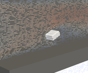
According to the description in § 3.4, the particle's movement is considered once pressure and velocity convergence have been determined. Figure 11 provides a visualization of the particle structure's transport starting from a position close to the inlet for five selected points in time, to be referred to hereafter as T1, T2, T3, T4 and T5. Initially, the particulate structure resides on the wall's surface enclosed tightly by the passing fluid. After release, it detaches and entrains into the flow while accelerating quickly. This entrainment is accompanied by a slow but steady upward motion towards the channel's upper wall. Owing to its irregular shape and the resulting varying flow conditions, it tumbles during its traversal through the channel. Right before hitting the back wall, it can be observed to decelerate while accelerating the nearby fluid in an otherwise nearly still surrounding fluid due to its momentum inherited from the previous acceleration.

Figure 11. Time series of detachment and transport of a particle structure inside the four-channel set-up. Inflow velocity of  $\bar {u}_{in}=1.0\ {\rm m}\ {\rm s}^{-1}$ and scaling factor of
  $s_l=0.2$.
The evolution of the particle velocity  $\boldsymbol {u}_p$ and the hydrodynamic force
  $\boldsymbol {F}$ are shown in figure 12 separated into their
  $x$ and
  $z$ components. The particulate structure's velocity increases immediately after release. The velocity in the
  $z$ direction exhibits an initial increase but drops to zero quickly after approaching the upper channel wall. The
  $x$ component, however, exhibits a distinct pattern of velocity increase, peak
  $u_{p,x,max}$ at
  $t_{max}$ and decrease before impacting the back wall at
  $t_{imp}$ with velocity
  $u_{p,imp}$. This behaviour is caused by the hydrodynamic forces acting on the structure's surface. It can be seen that the acceleration and deceleration phase can clearly be identified from the force in
  $x$ direction, which changes its sign by crossing the zero line at
  $t_{max}$. The force in the
  $z$ direction is much smaller and features a less distinct behaviour while fluctuating around zero. The initial values
  $F_{x,0}$ and
  $F_{z,0}$ characterize the structure's ability to detach from the filter surface. It can be observed that the initial force in the
  $x$ direction is much higher than that in the
  $z$ direction.

Figure 12. Transient behaviour of particle velocity  $\boldsymbol {u}_p$ and surface force
  $\boldsymbol {F}$ in
  $x$ and
  $z$ directions. Starting position of
  $x_{p,0}/l_{x,s}=0.05$, and particle density of
  $\rho _p=500\ {\rm kg}\ {\rm m}^{-2}$.
5.2. Detachment
The detachment of particulate structures inside a wall-flow filter channel is determined by the relation between the adhesive and the hydrodynamic forces acting on the particle's surfaces. A single detachment event can be caused by either increasing the hydrodynamic forces or reducing the adhesive ones. The former results from an increased flow rate or a greater exposure of the structure's surface. The latter can, on the one hand, be caused by a reduction of connecting soot matter due to its reaction during filter regeneration. On the other hand, it can be caused by a continuous exposure to hydrodynamic forces being on the verge of overcoming the respective adhesive contributions over a certain period of time. When considering multiple detachment events, another possibility is an increase of the surface force due to the direct momentum transfer of a colliding second structure.
Owing to those many mechanisms, the present work does not aim at assessing the occurrence of detachment events at this point. Rather, it provides insights into the borderline adhesive forces that need to be overcome for given flow conditions. In order to provide a close-up of the detachment process at T1 in the time series shown in figure 11, four successive time substeps T1a, T1b, T1c and T1d are selected and displayed in figure 13. Before release, the particulate structure rests flush on the filter wall at T1a. The passing flow circumvents the obstacle while slowing down right behind it. The detachment in T1b starts with a lift-off of the front surface and a subsequent tilting around its  $y$-axis. When fully erected in T1c, the structure exposes a large surface area opposing the main flow direction and reaches further into the core flow of higher velocities. This results in an increase in the hydrodynamic force, eventually causing the structure to separate from the surface in T1d and to resuspend into the gaseous flow.

Figure 13. Close-up of the detachment process of the particle structure from the porous filter wall. Inflow velocity of  $\bar {u}_{in}=1.0\ {\rm m}\ {\rm s}^{-1}$. Arrows (small and coloured in the background) indicate direction and magnitude of the local flow velocity.
In order to investigate the influence of the relative channel location, the transient behaviour resulting from a release at different starting positions  $x_{p,0}$ is examined. The course of the force's
  $x$ and
  $z$ components is shown in figure 14 for five exemplary positions. The development of the force
  $F_x$ directly reflects the observed behaviour described above. Right after release, the force increases due to the enlargement of the affected surface area reaching its maximum in T1c. The subsequent tumbling results in an oscillation, followed by a steep decrease due to a reduction of the relative particle velocity. For positions closer to the channel end, the absolute value decreases and the distinct pattern gradually evens out. Nonetheless, every position features a clear traversal from a positive to a negative force before hitting the back wall. The force in the
  $z$ direction is affected by the starting position similarly as the amplitude of the fluctuating behaviour gradually decreases.

Figure 14. Transient development of surface force  $\boldsymbol {F}$ in
  $x$ and
  $z$ directions for different starting positions
  $x_{p,0}$. Particle density of
  $\rho _p={500}\ {\rm kg}\ {\rm m}^{-3}$.
The detachment itself is mainly affected by the force at time  $t={0}\ {\rm s}$. The dependence of those initial values on the starting position is shown in figure 15. It becomes evident that the force in the
  $x$ direction exceeds that in the
  $z$ direction by at least a factor of four in every case, while both decrease towards the channel end. As described via (2.12a,b), those values stem from summing the force contributions at all boundary nodes and applying those to the particle's centre of mass. As the bottom surface is not accessible for the fluid, the individual contributions can act only on the particle's sides and its top surface. This uneven distribution results in a large torque around the
  $y$-axis, leading to the immediate tilt of the particle in T1b. It can therefore be reasoned that a detachment of particle structures with similar form will most likely be caused by a rotational movement due to the
  $x$-directed force contributions rather than the significantly smaller lift force in the
  $z$ direction.

Figure 15. Dependence of initial force value  $\boldsymbol {F}_0$ in
  $x$ and
  $z$ directions on the starting position
  $x_{p,0}$.
5.3. Transport
In order to evaluate a particle's behaviour while traversing along the channel, its current relative position in the channel  $x_p$ is mapped to the absolute channel position
  $x$ at the respective time
  $t$. Figure 16 shows the dependence of the particle's velocity in the
  $x$ direction on the current channel position for different starting positions
  $x_{p,0}$. The
  $x$ component of the position-dependent fluid velocity
  $\bar {u}_x$ for the particle free flow is added as well. Independent of the starting position, analogously to figure 12, the velocity can be seen to increase initially, but decrease towards the channel end. For starting positions approaching the channel's rear, however, both maximum velocity
  $u_{p,x,max}$ and impact velocity
  $u_{p,imp}$ become smaller. This behaviour can be directly attributed to the relative velocity between the position-dependent fluid velocity
  $\bar {u}_x$ and the particle velocity
  $u_{p,x}$, which can be derived directly from figure 16. Large differences in both velocities lead to large accelerations or decelerations, depending on their sign. Independent of the starting position, all particles are impacting the back wall with a velocity differing significantly from zero.

Figure 16. Particle velocity in the  $x$ direction
  $u_{p,x}$ for different starting positions
  $x_{p,0}$ at a density of
  $\rho _p=500\ {\rm kg}\ {\rm m}^{-3}$. The velocity profile
  $\bar {u}_x(x)$ of the particle-free case is shown as a reference.
In figure 10 a negligible dependence of the scaling factor  $s_l$ on the fluid velocity profile was shown for a permeability of
  $K=4.3\times 10^{-12}\ {\rm m}^{2}$. The respective relations for higher permeabilities and their impact on the dynamic behaviour of the particle structures are displayed in figure 17. The profiles of
  $\bar {u}_x$ for a scaling of
  $s_l=0.2$ share the same general behaviour as the full-length version displayed in figure 9; however, they show a smaller sensitivity to an increase of the substrate permeability. For higher permeabilities, the flow velocity decreases in the channel's front section and leads to smaller acceleration of a detached particle structure. Its impact velocity, however, additionally depends on the onset of deceleration, enabling particle structures to potentially approach the wall with a greater velocity despite its initially smaller acceleration (e.g. for
  $K=4.3\times 10^{-9}\ {\rm m}^{2}$). This shows that the permeability affects the structure's trajectories in a non-trivial manner and should therefore be chosen as close to a realistic value as possible. The following studies, therefore, exclusively consider a substrate permeability of
  $K=4.3\times 10^{-12}\ {\rm m}^{2}$.

Figure 17. Particle velocity in the  $x$ direction
  $u_{p,x}$ for different substrate permeabilities
  $K$ with starting position
  $x_{p,0}/l_{x,s}=0.05$. Respective velocity profiles
  $\bar {u}_x(x)$ of particle-free cases are shown as a reference.
The overall magnitude of the linearly decreasing axial flow velocity is determined by the inflow velocity  $\bar {u}_{in}$ which, in turn, directly dictates the profile of the axial particle velocity
  $u_{p,x}$. The extent of this influence is shown for two exemplary starting positions
  $x_{p,0}/l_{x,s}=0.05$ and
  $x_{p,0}/l_{x,s}=0.4$ in figure 18. Next to the expected differences in the trajectory's magnitude, a shift of the maximum velocity
  $u_{p,x,max}$ towards the channel's rear can be observed for greater inflow velocities. This exposes a longer acceleration time, leaving less remaining distance for the deceleration of the particle structure. This effect combined with the greater magnitude leads to increased impact velocities
  $u_{p,imp}$ at the channel end.

Figure 18. Particle velocity in the  $x$ direction
  $u_{p,x}$ for different inflow velocities
  $\bar {u}_{in}$ with exemplary starting positions
  $x_{p,0}/l_{x,s}=0.05$ and
  $x_{p,0}/l_{x,s}=0.4$.
The dependence on the particle density  $\rho$ is shown in figure 19 for the same starting positions. It can be observed that the particle structure density directly defines the intensity of acceleration and deceleration due to the relative velocity. While lower densities clearly lead to higher peak velocities, such a dependence does not hold for the impact velocity. A particle with a density of
  $\rho _p=100.0\ {\rm kg}\ {\rm m}^{-3}$ is able to quickly adapt to the surrounding fluid conditions. Despite its high peak velocity, it features a steep velocity decrease in the channel back, eventually resulting in a comparatively small impact velocity.

Figure 19. Particle velocity in the  $x$ direction
  $u_{p,x}$ for different densities with exemplary starting positions
  $x_{p,0}/l_{x,s}=0.05$ and
  $x_{p,0}/l_{x,s}=0.4$. The velocity profile
  $\bar {u}_x(x)$ of the particle-free case is shown as a reference.
In order to evaluate the impact of the particle density for different starting positions, the peak velocity  $u_{p,x,max}$ and the impact velocity
  $u_{p,imp}$ are retrieved for multiple simulations and displayed in figure 20. The same tendencies as discussed previously can be observed. The peak velocity decreases with both higher densities and advancing starting positions. The impact velocity generally decreases towards the channel end, but exhibits a less predictable behaviour for smaller densities. Studying the said parameter enables predictions for the packing density of accumulations at the channel end. It can, therefore, be assumed that particle structures detaching in the channel's front section are more likely to cause dense packings due to their elevated impact velocity.

Figure 20. Dependence of peak velocity  $u_{p,x,max}$ and impact velocity
  $u_{p,imp}$ on the starting position
  $x_{p,0}$ for different particle densities
  $\rho _p$.
Eventually the stopping distance  $\Delta l_{s}$, as introduced in § 2.4, is evaluated for different starting positions and particle densities. The distance to the back wall from the respective position of the maximum velocity
  $\Delta l_{w,max}$ is calculated as well. The resulting values are shown in figure 21. Owing to the constant mobility of
  $\mu _p=33.78\times 10^{6}\ {\rm s}\ {\rm kg}^{-1}$, the stopping distance exhibits the same characteristics as the peak velocity in figure 20. It can be observed that the stopping distance exceeds the remaining distance to the back wall significantly in every case. By means of this engineering-motivated parameter, it can be directly deduced that, within the range of the investigated parameters, a particle is very likely always to hit the back wall once detached. While the described studies were exclusively performed on a scaled channel geometry with length
  $l_{x,s}$, figure 21 reveals that the stopping distance even exceeds the unscaled total channel length
  $l_x$. This eventually proves the applicability of the scaling methodology, as it reduces computation times while being capable of leading to statements that are generalizable to the full-length set-up as well.

Figure 21. Dependence of stopping distance  $\Delta l_{s}$ and distance to wall in the
  $x$ direction at maximum velocity
  $\Delta l_{w,max}$ on the starting position
  $x_{p,0}$ for different particle densities
  $\rho _p$. The distance to the wall in the
  $x$ direction at starting position
  $\Delta l_{w,0}$ is shown as a reference. Guidelines at
  $l_x$ and
  $l_{x,s}$ indicate full and scaled channel lengths.
5.4. Comparison with experimental results
The plausibility of the presented results is assessed by comparing them to some exemplary ones retrieved from the experimental set-up (cf. § 3.2). Prior to the detachment experiments, a continuous particle layer is prepared from soot particles and glass spheres serving as ash replacement. The loaded channel is subsequently utilized to investigate the detachment and transport behaviour of individual agglomerates. While observing the entire model filter channel with a high-speed camera, a particle-free air flow with a defined inflow velocity at ambient conditions is routed through the filter. The inflow velocity is then slowly increased in small increments until individual agglomerates detach and are transported through the inlet channel. The discrete change in an agglomerate's position is extracted by determining its centre from the recording via image processing. Its size is determined by evaluating the longest chord of both length and width at the time of its detachment as a 2-D quantity. Owing to the single camera perspective, the thickness of such agglomerates cannot be specified.
Two experimental runs with different resulting particle dimensions ( ${500}\ {\mathrm {\mu }}{\rm m}\times 300\ {\mathrm {\mu }}{\rm m}$ and
  $800\ {\mathrm {\mu }}{\rm m}\times 400\ {\mathrm {\mu }}{\rm m}$) are considered within a comparison with simulation results. Both detachment events occurred at an inflow velocity of
  $\bar {u}_{in}={15.0}\ {\rm m}\ {\rm s}^{-1}$ close to the channel inlet. Owing to this high value, an inflow velocity of
  $\bar {u}_{in}={2.0} {\rm m}\ {\rm s}^{-1}$, representing the highest one considered in the present work, is used for the comparison. As a particle density of
  $\rho _p={100.0}\ {\rm kg}\ {\rm m}^{-3}$ leads to the most pronounced acceleration and deceleration behaviour (cf. figure 19) due to the smallest particle relaxation time according to (2.13), it is selected here.
The temporal velocity evolutions of all runs normalized by their respective peak velocities  $u_{p,x,max}$ are displayed in figure 22. In contrast to the inflow velocity considered in the simulation set-up, the inflow velocity causing detachment in the experimental runs of
  $\bar {u}_{in}={15.0}\ {\rm m}\ {\rm s}^{-1}$ is much higher. This difference can be directly attributed to the differing initial conditions, as the continuous layer surrounding the particle fractions increases adhesion and decreases the surface area accessible for the fluid flow. Additionally, the resulting agglomerate sizes are greater than the size of the particle structures of
  ${340}\ {\mathrm {\mu }}{\rm m}\times 170\ \mathrm {\mu }{\rm m}$ considered for the simulation set-up. Those differences, therefore, impede a comparison of the detachment behaviour. The particles’ transport characteristics can, however, be used within a qualitative comparison. Both experimental runs exhibit similar features to the simulation results presented above. After a steep increase in the fluid velocity, it reaches a maximum
  $u_{p,x,max}$, eventually decreases and hits the wall with a non-negligible velocity
  $u_{p,imp}$. The run closer to the inlet also exposes a higher peak velocity. Owing to the small number of data points at this moment, however, the discrete description of the velocity development is subject to high fluctuations.

Figure 22. Comparison of normalized particle velocity in the  $x$ direction
  $u_{p,x}/u_{p,x,max}$ between exemplary simulation and experimental results. Determination of
  $u_{p,x,max}$ of experimental runs was achieved by a polynomial fit to the data points.
6. Conclusion
This work investigates the detachment and transport behaviour of particle structures during filter regeneration with 3-D surface-resolved simulations using an LBM. First, the particle-free flow field inside a single wall-flow filter channel was analysed using two different simulation set-ups. The former allowed for a pressure drop comparison with experimental investigations and led to the determination of a physically sensible substrate permeability of  $K=4.3\times 10^{-12}\ {\rm m}^{2}$. With the second set-up, it could be shown that the permeability not only has an impact on the pressure drop, but also has a significant one on the velocity profiles, which can be differentiated by referring to the channel's front and its back section. The influence of the channel scaling on the form of the velocity profile could be shown to be negligible for a permeability of
  $K={4.3\times 10^{-12}}\ {\rm m}^2$. On this basis, the transient behaviour of single particle structures with a base size of
  ${170}\ {\mathrm {\mu }}{\rm m}$ and different densities was examined.
First, the general transport characteristics were determined, identifying several key parameters utilizable for a standardized comparison of different simulation and experiment runs. Those include the peak velocity, the impact velocity and the stopping distance. In order to assess the likelihood of a detachment from the channel surface, the hydrodynamic forces in tangential and normal flow directions were analysed. It could be shown that detachment is more likely caused by a rotational movement induced by tangentially oriented drag forces than by lift forces.
Lastly, the pneumatic transport of the particle structure through the channel was investigated for different starting positions, substrate permeabilities, inflow velocities and particle densities. It became evident that, within the range of considered parameters, the structures always hit the back wall with a non-negligible velocity. The substrate permeability could be shown to lead to non-trivial effects on the structure's trajectories, substantiating the necessity of the retrieval of a physically sensible permeability beforehand. Different densities of the particle structures could be observed to directly determine the ability to adapt to changing flow conditions. The stopping distance was shown to represent an accessible criterion for the structure's likelihood to impact on the back wall without the necessity of examining its exact trajectory. With it, it could be shown that, provided there is detachment from the channel surface, a particle structure is very likely always to hit the back wall. Experimental observations were then used to show qualitative accordance with the general movement characteristics.
The presented methodology and the respective results represent a step towards a universal and consistent formulation of the relation between relevant input quantities and the formation mechanisms of specific deposition patterns. This eventually enables predictions and modification recommendations regarding operating conditions that can be used to achieve optimizations in engine performance, fuel consumption and service life of wall-flow filters.
Acknowledgements
We would like to acknowledge the experimental project funded by the Deutsche Forschungsgemeinschaft (DFG, German Research Foundation), 438308378, on the ‘Experimental investigation of formation mechanisms and rearrangement phenomena of reactive–inert particle layers in cross-flow filters in gas cleaning applications’ for their support with the experimental results.
Funding
Funded by the Deutsche Forschungsgemeinschaft (DFG, German Research Foundation), 422374351.
Declaration of interests
The authors report no conflict of interest.
Author contributions
N.H.: Conceptualisation, methodology, software, validation, formal analysis, investigation, writing – original draft, project administration, visualisation, data curation. J.R.D.T.: Experimental investigation, writing – review and editing. J.M.: Experimental investigation, writing – review and editing. M.J.K.: Resources, software, supervision, funding acquisition, writing – review and editing. A.D.: Conceptualization, resources, supervision, funding acquisition, writing – review and editing.
Data availability statement
The implementation of all numerical models used in this work is available within the open-source software OpenLB.


 Open access