


1. Introduction
Glaciers are shrinking on the global scale at an accelerated rate in response to increasing air surface temperatures (Zemp and others, Reference Zemp2019). Widespread consequences are the contribution of glaciers to global sea-level rise (Jacob and others, Reference Jacob, Wahr, Pfeffer and Swenson2012; Zemp and others, Reference Zemp2019), the decline of glaciers as a source of water runoff used in the industry, households, agriculture and hydro-electrical power generation (Huss and Hock, Reference Huss and Hock2018; Quincey and others, Reference Quincey2018; Schaefli and others, Reference Schaefli, Manso, Fischer, Huss and Farinotti2019), and the increased threat for downstream natural disaster events (Kääb and others, Reference Kääb, Reynolds, Haeberli, Huber, Bugmann and Reasoner2005; Kääb, Reference Kääb, Singh, Singh and Haritashya2011; Wang and Zhou, Reference Wang and Zhou2017). In this paper, we focus on the Tien Shan mountain range in Central Asia. Consistent with the global trend, an accelerated retreat of glaciers in the Tien Shan has been observed during the last several decades (Solomina and others, Reference Solomina, Barry and Bodnya2004; Hagg and others, Reference Hagg, Mayer, Lambrecht, Kriegel and Azizov2013; Farinotti and others, Reference Farinotti2015; Petrakov and others, Reference Petrakov2016; Kraaijenbrink and others, Reference Kraaijenbrink, Bierkens, Lutz and Immerzeel2017; Shahgedanova and others, Reference Shahgedanova2020). In this region, glaciers are vital to the life of millions of people (Bolch, Reference Bolch2007; Immerzeel and others, Reference Immerzeel, van Beek and Bierkens2010; Sorg and others, Reference Sorg, Bolch, Stoffel, Solomina and Beniston2012; Pritchard, Reference Pritchard2019). During dry summers, when water sources such as snow melt have been depleted and precipitation is absent, glacial meltwater provides a crucial source of fresh water used for drinking and irrigation (Immerzeel and others, Reference Immerzeel, van Beek and Bierkens2010; Farinotti and others, Reference Farinotti2015; Kraaijenbrink and others, Reference Kraaijenbrink, Bierkens, Lutz and Immerzeel2017; Pritchard, Reference Pritchard2019). As such, the Tien Shan is considered as the water tower of the dry lowland areas of the surrounding countries (Luo and others, Reference Luo2018). Recent studies have demonstrated that at the end of this century, the water contribution of glaciers will be drastically reduced in this arid region (Immerzeel and Bierkens, Reference Immerzeel and Bierkens2012; Kraaijenbrink and others, Reference Kraaijenbrink, Bierkens, Lutz and Immerzeel2017; Luo and others, Reference Luo2018). Nevertheless, differences in the amount of glacier ice reduction and the sensitivity of individual glacier basins to climate change remain large.
To be able to make precise projections about future glacier volume and the evolution of glacier-fed runoff under global warming in the Tien Shan, accurate assessments of glacier ice thickness distributions are necessary. Because of the lack of direct measurements, multiple models have been developed and applied to derive the ice thickness distribution of a glacier from surface characteristics and the principles of ice flow dynamics (Huss and Farinotti, Reference Huss and Farinotti2012; Linsbauer and others, Reference Linsbauer, Paul and Haeberli2012; Frey and others, Reference Frey2014; Fürst and others, Reference Fürst2017; Ramsankaran and others, Reference Ramsankaran, Pandit and Azam2018; Maussion and others, Reference Maussion2019). These models have specifically been developed to be applied on regional (Fürst and others, Reference Fürst2018) to global scales (Farinotti and others, Reference Farinotti2019). Although these models consider available thickness observations, point measurements are not necessarily reproduced and large deviations are present, especially at the local scale. Moreover, differences between the individual reconstruction models are unsatisfying as a result of the scarcity of in situ measurements used for calibrating these models (Sorg and others, Reference Sorg, Bolch, Stoffel, Solomina and Beniston2012; Unger-Shayesteh and others, Reference Unger-Shayesteh2013; Kutuzov and others, Reference Kutuzov, Thompson, Lavrentiev and Tian2018; Farinotti and others, Reference Farinotti2019) and additional detailed ice thickness reconstructions based on measurements are needed. To date, the ice thickness of only a handful of glaciers in the Tien Shan is known from geophysical observations using a radio-echo sounding (RES) system, and most of them are located in the eastern areas of the Tien Shan (Hagg and others, Reference Hagg, Mayer, Lambrecht, Kriegel and Azizov2013; Zhen and others, Reference Zhen, Shiyin, Shiqiang and Honglang2013; Petrakov and others, Reference Petrakov, Kovalenko, Lavrentiev and Usubaliev2014; Wang and others, Reference Wang2014; Nosenko and others, Reference Nosenko, Lavrentiev, Glazovskii, Kazatkin and Kokarev2016; Pieczonka and others, Reference Pieczonka, Bolch, Kröhnert, Peters and Liu2018).
In the light of the existing limitations, we used RES to measure the ice thickness of Ashu-Tor, Bordu, Golubin and Kara-Batkak glaciers in the Kyrgyz Tien Shan, where few prior measurements of ice thickness exist. Here, we present all our in situ ice point thickness measurements (~1000 points). We extend these measurements to the entire glaciers using three different approaches based on the assumption of a constant yield stress (model 1) and on the principle of mass conservation (models 2 and 3). The three models are calibrated against the RES measurements. A cross-validation between modelled and measured ice thickness is performed for a subset of the data to assess the performance and to compose a weighted average optimal ice thickness distribution for every glacier. The latter can be used to (i) more accurately assess the glaciers total ice thickness distribution and associated ice volume, (ii) apply glacier evolution studies on a detailed scale and (iii) constrain ice thickness models developed to be applied in data-scarce regions. Furthermore, we compare the measurements and the composed ice thickness distribution with different ice thickness estimates and with the consensus estimate (Farinotti and others, Reference Farinotti2019), all constructed from models without the use of direct in situ field measurements. As part of our comparison, we explore how the use of these estimates could affect ice volume assessments and glacier evolution studies.
2. Location, fieldwork and ice thickness measurements
2.1 Study area
The four glaciers studied are located in the Kyrgyz part of the Tien Shan, which is a mountain range that stretches for over 3000 km from the east of Xinjiang, China, to the west of Tashkent in Uzbekistan (Fig. 1). The mountain range contains several reference glaciers with monitoring records dating back to the 1950s and 1960s (WGMS, 2019). At present, the glacier coverage is ~15 000 km2 with an estimated total ice volume of ~1000 km3 (Aizen and others, Reference Aizen, Kuzmichenok, Surazakov and Aizen2007; Farinotti and others, Reference Farinotti2015; Baojuan and others, Reference Baojuan, Weijun, Yetang and Zhongqin2017). The interaction between the atmospheric circulation associated with the Siberian high and the westerlies provides the mountain range with a more temperate climate in the western and northern part and a more continental climate in the central and eastern areas (Aizen and others, Reference Aizen, Aizen, Melack and Dozier1997).

Fig. 1. Map of the Tien Shan mountain range in Kyrgyzstan. The selected glaciers are located in two different regions (Western Tien Shan and Inner Tien Shan). The glacier outlines are taken from the Randolph Glacier Inventory (RGI) version 6.0 (RGI, 2020). Background: Hillshade from SRTM.
The four glaciers are all medium-sized valley glaciers and characterized by (long-term) glaciological monitoring programs maintained by different research institutes and in the framework of multiple projects. The first glacier is Golubin glacier, a medium-sized glacier, located in the Ala-Archa basin in the Kyrgyz Ala-Too range in the northwestern part of Kyrgyzstan. Surface mass-balance (SMB) measurements on this glacier were started by the Kyrgyz unit of the hydro-meteorological service of the USSR in 1958 and continued up to 1994 (Hagg and others, Reference Hagg, Braun, Uvarov and Makarevich2004). In 2010, SMB and length change measurements were reinitiated in the framework of the Capacity Building and Twinning for Climate Observing Systems (CATCOS) and Central Asian Water (CAWa) projects and they continue today (Kronenberg and others, Reference Kronenberg2016; Hoelzle and others, Reference Hoelzle2017; Barandun and others, Reference Barandun2018). The three other glaciers are located ~500 km to the east and are situated south of the large Issyk-Kul lake in the Inner Tien Shan. While Bordu glacier is located in the Ak-Shyirak massif, Ashu-Tor and Kara-Batkak glaciers are located in the Terskey Ala-Too. Nevertheless, Ashu-Tor glacier is positioned on the southern slopes, which is in the same plateau system as Bordu glacier (Arabel). This plateau is characterized by an annual precipitation of 300–400 mm primarily falling in summer (May–September). This implies that these glaciers receive most of the accumulation when ablation takes place (Khromova and others, Reference Khromova, Dyurgerov and Barry2003; Kronenberg and others, Reference Kronenberg2016). SMB measurements on Ashu-Tor and Bordu glaciers were initiated in 2014 and continue today. Kara-Batkak glacier is located on the northern slope of the Terskey Ala-Too range with a slightly higher total precipitation (Satylkanov, Reference Satylkanov2018). This glacier is significantly smaller than the three other glaciers. SMB measurements on this glacier started in 1947 and continued up to 1998. The measurements on this glacier were reinitiated in 2013 by the Tien Shan High Mountain Scientific Research Center as part of the CHARIS Project (Contribution to High Asian Runoff from Ice and Snow/Ice and snow contribution to the flow of High Asia) (Satylkanov, Reference Satylkanov2018).
2.2 Field campaigns and RES soundings
In August 2016, 2017 and 2019, field campaigns were accomplished to measure the ice thickness of the selected glaciers with a Narod RES system. This system has been applied in a very large number of studies to measure the ice thickness of mountain glaciers thanks to its ease of operation and its lightweight (Narod and Clarke, Reference Narod and Clarke1994; Fountain and others, Reference Fountain, Raymond and Nakao2000; Pattyn and others, Reference Pattyn2003; Zekollari and others, Reference Zekollari, Huybrechts, Fürst, Rybak and Eisen2013; Lambrecht and others, Reference Lambrecht, Mayer, Aizen, Floricioiu and Surazakov2014). The RES system works via a transmitter, which sends a radio wave that penetrates into the ice. A low frequency of 5 MHz was preferred to ensure a sufficiently large penetration depth of the radar signal and to limit the amount of attenuation due to disturbances in the glacier ice during summer (e.g. water inclusions). Such a low frequency ensures a clearer signal but results generally in a larger uncertainty of the measurements (lower vertical resolution, see Section 2.3). High frequencies on the other hand are often associated with a larger amount of signal attenuation and scattering but contain a higher vertical resolution. We anticipate that future field campaigns in Kyrgyzstan in winter or in spring can, in the absence of meltwater, use higher frequency RES systems (e.g. 10 or 20 MHz) with a lower error range in the measured ice thickness. Furthermore, unreachable areas in summer are likely more accessible during winter expeditions when the small crevasses are fully snow covered and a sledge radar system can be used. In addition, measurements can also be performed with airborne or heliborne systems (Gärtner-Roer and others, Reference Gärtner-Roer2014; Langhammer and others, Reference Langhammer, Grab, Bauder and Maurer2019).
The transmitted wave by the radar is reflected back from the glacier bed towards the surface and recorded by the receiver at a distance (d) from the transmitter. The time it takes for the wave (t) to get back to the surface is converted into the local ice thickness (H) using

with v ice being the velocity of the wave through ice (1.68 × 10⁸ m s−1) while the velocity of the signal in air (v air) is set at 3.00 × 10⁸ m s−1. GPS measurements of the exact locations of the transmitter and the receiver were made with a TRIMBLE GeoXH 3000, GeoXH 6000 and a GeoX7 and were differentially corrected afterwards (typical precision of 0.2 m) using correction stations (Kumtor or Bishkek). The ice thickness was measured along one or two central flowlines and along multiple transverse profiles covering at least the entire ablation area and, where accessible, parts of the accumulation area (green points in Fig. 2 and Table 1).

Fig. 2. Satellite image (Sentinel-2 true colour composite) of the different glaciers displaying the spatial distribution of the ice thickness points. The satellite images were acquired on 11/08/2019 for Ashu-Tor glacier, 27/07/2017 for Bordu glacier, 12/08/2019 for Golubin glacier and 27/07/2017 for Kara-Batkak glacier. The green points correspond to the GPR measurement locations. The red triangles correspond to the digitized additional points along the central flowlines in the unmeasured sections of the glaciers. The thin black lines are elevation contours from an adjusted DEM added for every 20 m. The thick black lines correspond to the 4000 m elevation contour.
Table 1. RES collection and main characteristics of the glaciers
The bed reflector was picked manually from the radargram by indicating the exact position of the reflected wave. Afterwards, the time interval between transmission and reception of the wave was determined and converted to the local ice thickness. In addition, a post-processing migration technique (Fig. 3) was implemented to filter out unrealistic measurements and replace them by more plausible solutions (Binder and others, Reference Binder2009; Andreassen and others, Reference Andreassen, Huss, Melvold, Elvehøy and Winsvold2015). In this way, the ice thickness was adjusted when the lowest point along an ellipse describing the possible reflection points was located inside the ellipse of the previous or next measurement along the profile. Evidently, it is impossible for the bedrock to be located at this depth because otherwise the neighbouring wave should have been reflected at the same point. These erroneous reflections are, for example, caused by large inconsistencies in the ice (rocks, water) and are removed to prevent an underestimation of the ice thickness (Lapazaran and others, Reference Lapazaran, Otero, Martín-Español and Navarro2016).

Fig. 3. Line intensity visualization of a transverse RES profile in the ablation area of Bordu glacier (left panel). Ellipses of four ice thickness measurements (right panel). The migration algorithm corrects the ice thickness from the first measurement since it lies inside the ellipse of the second measurement. The original ice thickness of the erroneous measurement is indicated by a red dot, the corrected thickness is indicated by a green dot, the original and correct ice thicknesses of the other measurements are indicated by a blue dot.
2.3 Error of ice thickness measurements
Concerning the estimation of the error associated with the thickness measurements, we follow the terminology in Lapazaran and others (Reference Lapazaran, Otero, Martín-Español and Navarro2016). Since the location of the RES was measured using a differential GPS, and the GPR was stationary with a positional accuracy of ~0.2 m in rather flat areas, we assume the horizontal error related to the exact positioning to be much lower than the error related to the ice thickness measurement itself (εHgpr). The latter depends primarily on the used radar wave velocity (RWV = c) and the timing of the reflected wave with τ – two-way travel time. This error can be written as:

with $\lpar {\rm \epsilon }_\tau \rpar$ being the timing error and (εc) being the error related to the RWV. We used a constant RWV for all calculations, which can be justified since we mainly performed measurements in the ablation areas that consist of clean ice and with an absence of firn and/or snow. The uncertainty introduced by this assumption is correlated with the ice thickness and the exact temperature of the ice. As the selected glaciers are likely polythermal glaciers, similarly to Sary-Tor glacier with warm ice at the base and cold ice on top of it (Petrakov and others, Reference Petrakov, Kovalenko, Lavrentiev and Usubaliev2014; Nosenko and others, Reference Nosenko, Lavrentiev, Glazovskii, Kazatkin and Kokarev2016), the error is expected to be of the order of 1–2% of the reconstructed ice thickness (Lapazaran and others, Reference Lapazaran, Otero, Martín-Español and Navarro2016; Lippl and others, Reference Lippl2019). The timing error $\lpar {\rm \epsilon }_\tau \rpar$
 , a measure of how precisely the reflection can be determined in a RES record, is typically expressed as a function of the used frequency of the radar signal and is generally assumed to be constant for all measurements along a profile (Fountain and others, Reference Fountain, Raymond and Nakao2000). This error (often called the vertical resolution) is typically one-quarter of the wave-length of the used radar wave (Brandt and others, Reference Brandt, Kohler and Lüthje2008; Mouginot and others, Reference Mouginot, Rignot, Gim, Kirchner and Le Meur2008; Fischer, Reference Fischer2009; Gärtner-Roer and others, Reference Gärtner-Roer2014; Lambrecht and others, Reference Lambrecht, Mayer, Aizen, Floricioiu and Surazakov2014), which in our case corresponds to ~8 m. The error associated with all the measurements appears thus to be almost completely determined by the error associated with the detection of the reflected wave and only limited by the assumption of constant RWV. We characterize the error of the measurements further in this research accordingly as 8 m ± 2% of the measured ice thickness.
2.4 Result of measured ice thicknesses
After carefully analysing the different RES records, 981 point measurements could be used (Table 2 and Fig. 4). The RES records where the onset of the reflected wave could not be clearly recognized visually, due to a high level of distortion on the radar wave, were removed to prevent an incorrect ice thickness determination. We measured the thickest ice on Ashu-Tor with values up to 201.34 ± 12.02 m. This corresponds to the thickest ice that has been measured in the study area so far (Engel and others, Reference Engel, Šobr and Yerokhin2012; Hagg and others, Reference Hagg, Mayer, Lambrecht, Kriegel and Azizov2013; Petrakov and others, Reference Petrakov, Kovalenko, Lavrentiev and Usubaliev2014, Reference Petrakov2016). The maximum ice thickness (Table 2) was measured along the central flowline of Ashu-Tor glacier, close to the ELA where the slope is gentle.

Fig. 4. Histogram of the RES ice thickness measurements performed on every glacier. The bin size is 10 m.
Table 2. Total number of measurements and maximum measured ice thickness of the different glaciers
The maximum measured ice thickness of the other glaciers appears to be significantly lower. The measurements revealed a maximum value of 147.90 ± 10.96 m for Bordu glacier in the Ak-Shyirak mountain massif. The latter maximum is similar to the reported values of Sary-Tor glacier and glacier No. 354 in the neighbouring valleys (Hagg and others, Reference Hagg, Mayer, Lambrecht, Kriegel and Azizov2013; Petrakov and others, Reference Petrakov, Kovalenko, Lavrentiev and Usubaliev2014) and to the modelled ice thickness of Bordu glacier using the GlabTop model (Petrakov and others, Reference Petrakov2016). Furthermore, the RES measurements of Golubin glacier have a maximum of 154.05 ± 11.08 m. This is in the same order as the maximum ice thickness measured on Adygene glacier (~140 m), located in the neighbouring valley (Lavrentiev and others, Reference Lavrentiev2014). However, the maximum ice thickness might be reached in the areas where no measurements were performed, in the gently sloping accumulation area. Lastly, the measurements on Kara-Batkak glacier indicated the thinnest ice with a maximum ice thickness of 113.9 ± 10.28 m. This rather thin ice is closely related to the steepness of Kara-Batkak glacier characterized by multiple ice falls at different elevations. This is in line with the plastic flow law that relates ice thickness directly to the surface slope (Zekollari and others, Reference Zekollari, Huybrechts, Fürst, Rybak and Eisen2013).
2.5 Glacier outlines and surface elevation
The outlines of the four glaciers available in the RGI6.0 dataset of 2002 are updated to match the date of the outlines with the glacier margin at the date of the field campaigns. During the field campaigns, the frontal areas of the glaciers (except for Kara-Batkak glacier) were mapped using a DJI Phantom 4 Pro and a DJI Mavic to find the exact location of the glacier front and to produce a digital elevation model (DEM) of the glacier forefield (Fig. 5).

Fig. 5. The glacier front and forefield were mapped with a UAV to produce a DEM and to obtain an extension of the modelled bedrock field. The surface represents the surface elevation in the year of the field campaigns (2017/2019).
Plastic orange squares (40 × 40 cm) and well-definable individual boulders were used as ground control points (GCP) to georeference the created Digital Surface Models (DSMs) by manually marking them in Pix4D. Following guidelines in the literature (Gindraux and others, Reference Gindraux, Boesch and Farinotti2017), we obtained a GCP density of at least 6 GCPs km−2 in the frontal areas. The glacier outlines are accordingly updated using optical satellite data from Sentinel-2 with a spatial resolution of 10 m for the main glacier area and using the drone imagery with a spatial resolution of 5 cm for the glacier front delineation. Concerning Kara-Batkak glacier, only satellite data are used. Especially for the debris-covered areas and the accumulation areas of the glaciers, specific attention is given to the adjustment of the outlines since the RGI6.0 outlines appeared to mismatch the glacier extent in these areas (dashed lines in Fig. 2). Here, the use of the RGI6.0 outlines would significantly underestimate the total glacier ice volume due to an underestimation of the total glacial area (Racoviteanu and others, Reference Racoviteanu, Paul, Raup, Khalsa and Armstrong2009; Paul and others, Reference Paul2013; Nagai and others, Reference Nagai, Fujita, Sakai, Nuimura and Tadono2016). The TerraSAR-X add-on for Digital Elevation Measurement mission (TanDEM-X) (2013) is selected to represent the base representation of the glacier's surfaces. More recent DEMs such as the High Mountain Asia (HMA) DEMs (Shean and others, Reference Shean2020) still contain artefacts spread over the glacier surfaces. Furthermore, the three models that are applied (Section 3) are mainly calibrated with locally averaged surface slope values that did not change significantly over the period of interest. The original TanDEM-X data are transformed into the projected coordinate system UTM44N (suitable between 78°E and 84°E) for Ashu-Tor, Bordu and Kara-Batkak glaciers and UTM43N (suitable between 72°E and 78°E) for Golubin glacier and interpolated to a regular grid of 25 × 25 m using triangulation-based cubic interpolation. To correctly calculate the bedrock elevation from the ice thickness field, the elevations over the glacier area are adjusted for ice melt to match the date of the field campaigns. To do this, we first obtain average annual dh/dt rates from the difference between the TanDEM-X DEM (2013) and the SRTM DEM (2000) over the entire glacier areas, see also Section 3.1.2. Then, we extrapolate the TanDEM-X DEM from 2013 to 2017 for Bordu and Kara-Batkak glaciers and to 2019 for Ashu-Tor and Bordu glaciers by subtracting the mean dh/dt rates for the number of years until the year of the field campaigns. In the frontal areas (except for Kara-Batkak glacier), the surface DEM for the year of the field campaigns is derived from the photogrammetrically created DSMs from the UAV images (Fig. 5).
3. Ice thickness modelling in unmeasured areas
The spatial distribution of the ice thickness measurements shows that a substantial part of the glaciers was inaccessible during the field campaigns, especially in the accumulation areas (Fig. 2). Large crevasses, snow bridges, steep surfaces and changeable weather conditions inhibited access in these areas. Therefore, interpolation of the measured point ice thickness is required to obtain a glacier-wide ice thickness field. Direct interpolation between the measurements can be applied in the ablation areas but results in unrealistic extrapolation effects in the accumulation areas where in situ data are missing. Hence, we apply three different ice thickness models (c.f. yield stress model, mass flux flowline model, mass flux 2D model) to reconstruct the ice thickness over the entire glaciers on a regular grid of 25 × 25 m. The different input data of the three models are listed in Table 3. More details about the model's setup are given in the following sections.
Table 3. Overview of the different input data required by the applied models

3.1 Ice thickness modelling
The first two models initially reconstruct the ice thickness at points along predefined glacier central flowlines (red points in Fig. 2). The ice thickness at these points is then interpolated between the flowlines and the margin to obtain a continuous gridded ice thickness field, using the ANUDEM algorithm developed by Hutchinson (Reference Hutchinson1989). This algorithm has been designed to create a continuous surface mimicking the parabolic shape of a glacier bed from point measurements and has been applied in many studies (Fischer, Reference Fischer2009; Linsbauer and others, Reference Linsbauer, Paul and Haeberli2012). In the interpolation process, all the transverse ice thickness measurements are taken into account to optimize the quality of the entire ice thickness distribution. The ice thickness at the marginal gridpoints is set to 5 m representing the ice thickness at ~12.5 m from the margin, as was done in Zekollari and others (Reference Zekollari, Huybrechts, Fürst, Rybak and Eisen2013). The uncertainty that is introduced by defining the location (and associated catchment area) of the flowlines and following interpolation using ANUDEM is absent for the mass flux 2D model, which immediately reconstructs the ice thickness over the entire catchment area (Fürst and others, Reference Fürst2017).
3.1.1 Yield stress model
The first model is based on the perfect-plasticity assumption and constant yield stress and builds on the models described in Linsbauer and others (Reference Linsbauer, Paul, Hoelzle, Frey and Haeberli2009, Reference Linsbauer, Paul and Haeberli2012); Li and others (Reference Li, Ng, Li, Qin and Cheng2012) and Zekollari and others (Reference Zekollari, Huybrechts, Fürst, Rybak and Eisen2013). In this model, the basal shear stress along the central flowlines is set equal to an average yield stress (τ y) which is calibrated with the measured ice thicknesses based on the following relations:


with α the local surface slope and ρ the average ice density (900 kg m−3). Following Li and others (Reference Li, Ng, Li, Qin and Cheng2012) and Pieczonka and others (Reference Pieczonka, Bolch, Kröhnert, Peters and Liu2018), a shape factor (f) is introduced to account for the drag by the valley walls. For simplicity, we assume a constant of 0.8, similar to the value used for the consensus estimate (Farinotti and others, Reference Farinotti2019) and in the parametrization scheme of Haeberli and Hoelzle (Reference Haeberli and Hoelzle1995). This shape factor accordingly does not influence the ice thickness calculations (because it is kept constant) but produces more realistic basal shear stresses for a mountain glacier. We applied an averaging filter to prevent local topographical irregularities to dominate and minimize the spatial variability of the derived yield stresses. As such, we replaced the slope at a particular gridcell by the average slope of a window of 250 × 250 m centred over the gridcell, following Binder and others (Reference Binder2009). Then, for all unmeasured point locations along the central flowlines situated within 200 m from a radar measurement, the yield stresses are determined by interpolating between the measured yield stress at the radar measurements and the calculated average yield stress $\lpar \bar{\tau }_{\rm y}\rpar$ . For all other locations, the mean is ascribed directly. Afterwards, the local ice thickness is inferred from Eqn (5).

Previous studies showed that Eqn (5) tends to overestimate the ice thickness in very flat regions (small slope). Therefore, we implemented a minimum slope of 5% (Farinotti and others, Reference Farinotti, Huss, Bauder, Funk and Truffer2009, Reference Farinotti2017; Carrivick and others, Reference Carrivick, Davies, James, Quincey and Glasser2016; Pieczonka and others, Reference Pieczonka, Bolch, Kröhnert, Peters and Liu2018). However, we do not observe slopes smaller than 5% at the reconstruction points. In addition, as a test, we also derive the average yield stress for the four glaciers using the empirical equation of Haeberli and Hoelzle (Reference Haeberli and Hoelzle1995), with h range being the difference between the maximum and the minimum elevation of the glacier (Eqn (6)).

This equation was determined on the examination of the bedrock of 62 formerly existing late-glacial ice bodies of ice in the European Alps and is often used in the literature to estimate the uniform yield stress of a particular glacier (e.g. GlabTop model) lacking in situ measurements (Linsbauer and others, Reference Linsbauer, Paul, Hoelzle, Frey and Haeberli2009, Reference Linsbauer, Paul and Haeberli2012; Li and others, Reference Li, Ng, Li, Qin and Cheng2012). Table 4 shows that the calculated yield stresses of the four glaciers are typically of the order of 100–130 kPa. The rather large values are suggesting a cold structure of the glaciers. Kara-Batkak glacier is characterized by the largest average yield stress, which is associated with its range and its steepness (see Table 1). The value of 90.75 kPa for Bordu glacier is somewhat lower than the average yield stress value of 100 kPa found for glacier No. 354 (Hagg and others, Reference Hagg, Mayer, Lambrecht, Kriegel and Azizov2013). This might be the result of the smaller amount of RES soundings in the central area on glacier No. 354. Table 4 also indicates that the std dev. of the calculated yield stresses $\lpar \sigma _{\tau _{\rm y}}\rpar$ is particularly large for Kara-Batkak and Bordu glacier (28% of its mean value). Due to this variation, the assumption of a constant yield stress along the glacier flowlines does not seem to be valid for these glaciers. This is likely to result in a higher uncertainty of the derived ice thickness for the yield stress model. Nevertheless, Haeberli and Hoelzle (Reference Haeberli and Hoelzle1995) found a similar spread of data points for shear stresses (30–45%) reflecting the general variability of flow dynamics. For the other glaciers, but especially for Ashu-Tor glacier, the derived yield stresses fall into a narrower range (smaller σ).
Table 4. Average yield stresses and the associated std dev. of the yield stresses of all measurements derived for the four glaciers (values in kPa)

The empirically derived yield stress for every glacier is based on the equation of Haeberli and Hoelzle (Reference Haeberli and Hoelzle1995).
Next to that, the empirically determined average yield stress is lower for three of the four glaciers, which implies that using this stress would lead to an underestimation of the ice thickness (Table 4). This is opposite to the study of Marshall and others (Reference Marshall2011) who found that this value tends to overestimate the shear stress for small glaciers. Only for Bordu glacier, the use of this empirically determined stress would substantially overestimate the ice thickness. The deviation between the observationally and the empirically determined yield stresses might suggest that a different empirical relation holds for regions where the glaciers are polythermal, as is the case for other glaciers in the Tien Shan (Osmonov and others, Reference Osmonov, Bolch, Xi, Kurban and Guo2013; Petrakov and others, Reference Petrakov, Kovalenko, Lavrentiev and Usubaliev2014; Nosenko and others, Reference Nosenko, Lavrentiev, Glazovskii, Kazatkin and Kokarev2016).
3.1.2 Mass flux flowline model
The second model is based on Farinotti and others (Reference Farinotti, Huss, Bauder, Funk and Truffer2009). This model has been used extensively to reconstruct the ice thickness of glaciers worldwide (Huss and Farinotti, Reference Huss and Farinotti2012; Farinotti and others, Reference Farinotti2019) and for regional applications in, for example, Norway (Andreassen and others, Reference Andreassen, Huss, Melvold, Elvehøy and Winsvold2015) and Austria (Helfricht and others, Reference Helfricht, Huss, Fischer and Otto2019). The principle is to combine knowledge of the SMB $\lpar \dot{b}\rpar \;$ and surface elevation change rates (dh/dt) to find the balancing flux divergence $\nabla .q$
 via the conservation of mass equation and infer subsequently the ice thickness from this flux divergence:

First, the linear glacier-specific mass-balance gradients are calculated separately for the ablation and accumulation area from point stake and snow pit measurements. Concerning Ashu-Tor, Bordu and Kara-Batkak glaciers, SMB measurements are acquired via the framework of the CHARIS project (see Section 2.2) while for Golubin glacier, the data are obtained from the CATCOS and CAWa projects. Because the SMB measurements on Ashu-Tor glacier were only performed in the ablation area up to now (and for a limited number of stakes), we prefer to take the average of the gradients of Kara-Batkak and Bordu glaciers to represent the gradients of Ashu-Tor glacier, which is located in between. The different gradients and the estimated ELA are shown in Table 5. A small ablation gradient is obtained for Kara-Batkak and Bordu glaciers, in between values found in the past for Sary-Tor glacier (Ushnurtsev, Reference Ushnurtsev1991), Davydov (Aizen and Zakharov, Reference Aizen and Zakharov1989) and Batysh-Sook glacier (Kenzhebaev and others, Reference Kenzhebaev2017) and the average gradient of glacier No. 354 glacier (Kronenberg and others, Reference Kronenberg2016).
Table 5. SMB gradients of the ablation and the accumulation area of the different glaciers (in m.w.e/1000 m) and the estimated altitude of the equilibrium line (m)

The rather small gradients are typical for glaciers located in areas with a continental climate characterized by limited annual precipitation. According to Dyurgerov and others (Reference Dyurgerov1994), a change towards larger SMB gradients might be caused by climate change in the area. The accumulation gradient of Bordu glacier appears to be very small, which corresponds to the low amount of precipitation in the Ak-Shyirak massif. For Kara-Batkak glacier, we derive an accumulation gradient of +2.05 m.w.e/1000 m up to 4150 m and −2.82 m.w.e/1000 m above this altitude. Such a negative gradient is often observed in the highest parts of glaciers as a result of a decreasing amount of precipitation, changing wind patterns or the steepness of the surface. Golubin glacier appears to have a steeper ablation gradient, close to 8 m.w.e/1000 m, which is associated with the higher annual precipitation in the western part of the Tien Shan (~700 mm a−1). We find an accumulation gradient of 2.06 m.w.e./1000 m for Golubin glacier up to 4150 m and −1.17 m.w.e./1000 m above 4150 m. Subsequently, the apparent mass balance (AMB ~$\tilde{b}$ in m.w.e) is calculated using the glacier-specific ablation/accumulation gradients and average surface elevation change rates (dh/dt) over the entire glaciers (Eqn (8)). The latter are computed by smoothing average dh/dt rates from the difference between the SRTM DEM (2000) and TanDEM-X (2013). TanDEM-X data and associated dh/dt rates with respect to SRTM are processed following the workflow in Braun and others (Reference Braun2019), Farías-Barahona and others (Reference Farías-Barahona2020) and Sommer and others (Reference Sommer, Malz, Seehaus, Zemp and Braun2020). As discussed in these studies, radar penetration of the C-band SRTM product is taken into account by imposing a maximum 5 m penetration depth for the highest part of the glaciers, increasing linearly starting from 0 m at the 10% percentile of the glacier's elevation range. For the TanDEM-X DEM, surface penetration is assumed to be negligible compared to the general measurement accuracy. As such, errors on the dh/dt product due to radar penetration can be expected to be very small.

In the approach of Farinotti and others (Reference Farinotti, Huss, Bauder, Funk and Truffer2009), debris cover is taken into account by decreasing the AMB with 50% for cells covered with debris. However, for the selected glaciers, the extent of debris cover is limited (see Fig. 2) and we decided to not incorporate the debris. In the following step, the ELA is varied gradually (changing the local SMB) while keeping the dh/dt fixed until the catchment (defined for every individual flowline) wide ice volume flux equals zero (Farinotti and others, Reference Farinotti, Huss, Bauder, Funk and Truffer2009). The ice volume flux through every point along the central flowlines is then directly calculated by cumulating all the AMB values of the glacier catchment area upstream of the considered point contributing to the flow through the concerning point. Then, the ice volume flux is normalized by dividing the cumulative flux by the glacier effective width (w c) to obtain the mean specific ice volume flux for the cross-section of the glacier $\lpar \bar{q}_1\rpar$ (Eqn (9)) with n being all the grid cells upstream of the considered point. The glacier effective width is manually derived for every point measurement along the central flowlines following Farinotti and others (Reference Farinotti, Huss, Bauder, Funk and Truffer2009).

Finally, the ice thickness is inferred from the calculated mean specific ice volume flux using Glen's flow law and the Shallow Ice Approximation (SIA) with α being the slope averaged over an area of 250 × 250 m (similar as for the yield stress model) with a flow parameter (A) of 2.4 × 10⁻¹⁵ kPa−3s−1 and n = 3 the exponent in Glen's flow law:

C is a correction factor, taking into account all uncertainties in the coefficients and is calibrated using the measured ice thicknesses. In contrast to Huss and Farinotti (Reference Huss and Farinotti2012), we do not introduce a specific factor applying for basal sliding since it is considered to be taken into account in the correction factor. We findvalues of C between 0.13 (Ashu-Tor glacier) and 0.30 (Golubin glacier), which is lower than the values found for four glaciers in Switzerland (Farinotti and others, Reference Farinotti, Huss, Bauder, Funk and Truffer2009). Similar to the yield stress model, we impose a minimum slope of 5° to prevent an overestimation of the ice thickness in very gentle areas. Finally, the modelled thicknesses are ascribed to the unknown points of the flowlines.
3.1.3 Mass flux 2D model
Similar to the second model, the third approach to reconstruct glacier ice thickness is also based on the principle of mass conservation. Model 3 is informed by the central and transverse profiles to calibrate its parameters. The approach and its performance have been assessed for different glacier types on Svalbard (Fürst and others, Reference Fürst2017). It further participated in the ITMIX project (Farinotti and others, Reference Farinotti2017), was applied on regional scales for the Svalbard archipelago (Fürst and others, Reference Fürst2018) and contributed to the consensus estimate for mapping the glacier thickness distribution worldwide (Farinotti and others, Reference Farinotti2019). Unlike the first two models, this model directly computes the ice thickness distribution over the entire domain and not along predefined central flowlines. First, the AMB is derived from the linear mass-balance gradients presented in Table 5 and the surface elevation change rates between Tan-DEM-x and SRTM data. As no velocity information was available, the approach then infers the ice flux direction and magnitude. The flux is set to zero at the lateral margins (both parallel and perpendicular). During an iterative procedure, the AMB is adjusted to minimise a cost function that favours positive and smooth solutions and that penalises differences to the input AMB. This reduces undesired characteristics in the flux field resulting from inconsistencies in the input fields and anticipates a smoothed flux field (Fürst and others, Reference Fürst2017). To account for longitudinal coupling, a local and thickness-dependent smoothing is applied to the vector fields of the surface slope and the ice flux. In the mass flux 2D model, the flow parameter (A) is computed based on the individual ice thickness measurements and extrapolated over the entire glacier domain. A mean value of A is prescribed along the glacier margins to avoid unreliable extrapolation effects. In the last step, the glacier wide flux values are locally translated into thickness values assuming the SIA, similar to Eqn (10). For further details, the reader is referred to Fürst and others (Reference Fürst2017).
3.2 Model performance
We quantify the performance of each model by comparing modelled and measured ice thicknesses. The models are calibrated with a randomly selected fraction of the total number of the ice thickness measurements. Subsequently, the modelled ice thicknesses are compared with the measured ice thicknesses for the withheld (not used for calibration) points. As metrics, the mean absolute error (MAE) and the standard error of the estimate (SEE) are used. The MAE is defined as the absolute difference between the modelled and the measured ice thickness while SEE takes into account the variance of the errors. Twenty performance experiments are performed for each model concerning five times 25, 50, 75 and 90% of the measured ice thicknesses randomly withheld.
Clearly, the MAE and the SEE gradually increase when the percentage of withheld measurements is increased for all glaciers and all models (Fig. 6). However, overall, the MAE and SEE remain below 20%, which is satisfactory for most purposes. This implies that the ice thickness models estimate the ice thickness at the location of the withheld measurements with an accuracy of ±20%. Concerning Kara-Batkak glacier, however, the MAE and SEE are larger, especially for the yield stress model. This is in line with the larger variability (σ of 34 kPa) of the stresses calculated based on the measurements (Table 3). This suggests that this model assuming a constant yield stress is less appropriate to apply on Kara-Batkak glacier. This might reflect a larger variability of the flow dynamics (e.g. amount of basal sliding, ice deformation factor) (Linsbauer and others, Reference Linsbauer, Paul and Haeberli2012). For Bordu glacier, the difference between the performance of the yield stress model mass flux flowline model is smaller. All these findings suggest that the performance of glacier ice thickness models depends strongly on the glacier type and its characteristics. After all, Ashu-Tor glacier consists of a single glacier tongue while the shape of Kara-Batkak glacier is more complex and the glacier surface is significantly steeper. For all glaciers and all runs, the mass flux 2D model scores the lowest MAE and SEE. This demonstrates the overall best performance of this model for our dataset. Moreover, this hints for a more accurate ice thickness modelling when the mass flux is calculated in 2D instead of along central flowlines followed by an interpolation of the ice thickness using the ANUDEM algorithm (as is the case for the mass flux flowline model).

Fig. 6. Barplots of the mean absolute error (left) and standard error of the estimate (right) for the different percentages of withheld measurements. The units are in percentage. Blue = yield stress model, red = mass flux flowline model and yellow = mass flux 2D model.
3.3 Assembling composite ice thickness distribution
Following Poisson's law of large numbers, an ensemble of different models is assumed to produce optimal results of ice thickness estimates since the average converges to the expected value. This was also observed by Farinotti and others (Reference Farinotti2017) in the ITMIX project. Based on the observations, up to five models were combined into a consensus estimate for the ice thickness of all glaciers on Earth (Farinotti and others, Reference Farinotti2019). Following this procedure, we combine the three ice thickness distributions calibrated with all the measurements, created with the three models described in Section 3.2, into a composite ice thickness distribution for the selected glaciers. Based on the results discussed above, the mass flux 2D model performs better in areas with measurements. However, the mass flux 2D model might not perform better than the other approaches in areas where no thickness measurements were acquired. Similar to the approach in Farinotti and others (Reference Farinotti2019), a weight (w i) is attributed to every model based on the mean absolute error (MAE) and the variance (SEE2) (Eqn (11)). The MAE and SEE corresponding to the version of the selection of 75% withheld points are used.

The final contribution (in percentage) of every model to the composite ice thickness field is shown in Table 6. Because of the significantly lower MAE and SEE of the mass flux 2D model, this model accounts for ~60% of the composite ice thickness fields. The two other models are fairly equally weighted, except for Ashu-Tor and Kara-Batkak glaciers for which the yield stress model contributes substantially less.
Table 6. Contribution of the different models for every glacier

Subsequently, the three ice thickness fields including all measurements are merged and the final ice thickness at every gridcell (H i) is obtained using Eqn (12) with h being the ice thickness at a particular gridcell and H the composite ice thickness at the gridcell.

3.4 Ice thickness modelling error estimate
At the location of the RES measurements, the error of the ice thickness distribution equals the error of the measurements themselves, which is 8 m ± 2% of the measured ice thickness (see Section 2.3). Regarding the areas with a high density of RES measurements (especially the ablation areas), the error of the ice thickness estimates depends on the measurement's accuracy and the interpolation procedure. Because the density of RES measurements in these areas is high (glacier tongues), the MAE of the 50% withheld points is taken to represent the error. Figure 6 reveals a MAE of ~10%. In the areas without any RES measurements, the estimated ice thickness is accompanied by larger errors. Here, the potential errors are more difficult to estimate since the approach to compare modelled versus measured ice thicknesses cannot be applied. Therefore, we rely directly on the error characterization of the applied models and the MAE derived from the cross-validation test for the 90% withheld points. The latter corresponds to the largest error estimates with only 10% of the measurements used and corresponds to a very low density of ice thickness measurements for calibration. Combining all these values for the different glaciers would result in an average error of 10–15% for Ashu-Tor glacier, 15–20% for Bordu and Golubin glaciers and 20–25% for Kara-Batkak glacier. However, the mismatch calculated from this comparison likely underestimates the maximum local error in modelled ice thicknesses. It was found by Fürst and others (Reference Fürst2017) that ice thicknesses are strongly spatially correlated implying that the MAE and SEE found in the cross-validation tests are probably too low to extend directly to the unmeasured areas. Therefore, it is suggested to take the mentioned upper bounds as the best indication for the error.
4. Ice thickness distribution of Ashu-Tor, Bordu, Golubin and Kara-Batkak glaciers
4.1 Composite ice thickness distribution and glacier volumes
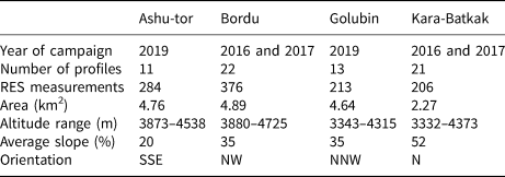
The final composite ice thickness distributions are displayed in Figure 7. Ashu-Tor glacier is clearly characterized by the thickest ice in the central part of the glacier, along the glacier centreline, with thicknesses of up to 200 m. The ELA is located in this rather flat area. Towards the glacier snout and towards the accumulation area, the ice thickness gradually declines. Furthermore, near the valley sides, the ice thickness decreases rapidly at similar rates on both valley sides (Fig. 7). The ice thickness of Ashu-Tor glacier is minimal at the highest parts of the accumulation area where the ice flux is limited, and the surface is steep (at the margin). Glacier volume (Table 7) is calculated to be 0.389 ± 0.078 km3 taking into account the potential errors discussed in Section 3.4. For Bordu glacier, central parts show characteristic thickness values of 60–120 m. This coincides with the large flat body of the glacier, which is in line with the plastic flow assumption relating ice thickness inversely to the surface slope (see Eqn (5)). Bordu glacier is characterized by generally steeper marginal zones in the accumulation areas (strong gradient in elevation contours), which results in minimum ice thickness in these parts. This matches closely to the modelled ice thickness distribution using the GlabTop model and surface elevations from SRTM and ASTER (Petrakov and others, Reference Petrakov2016).
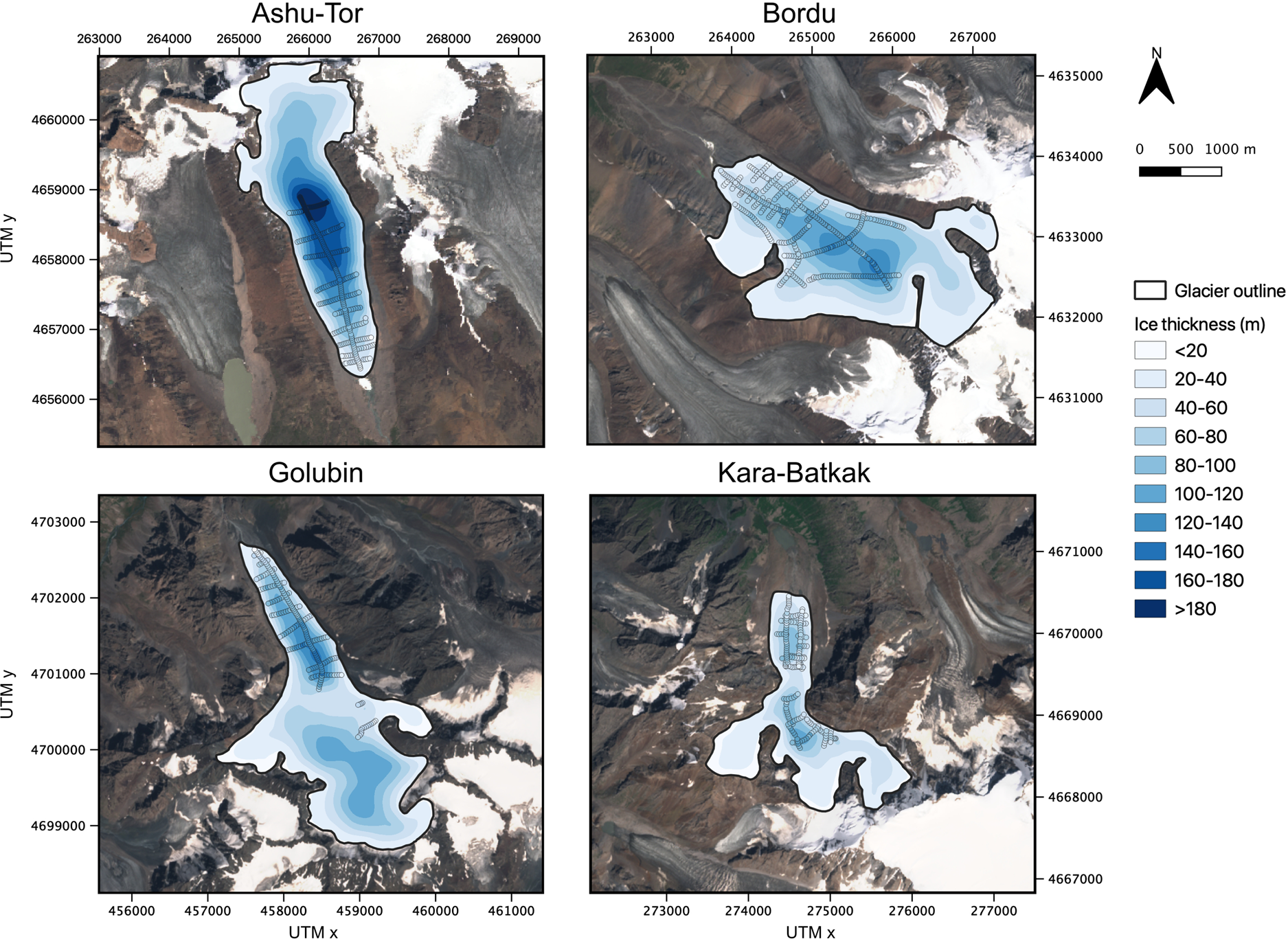
Fig. 7. Composite ice thickness of the four glaciers. The locations of the ice thickness measurements are indicated with a circle. The colour of the circles corresponds to the measured ice thickness.
Table 7. Ice volumes of the composite ice thickness distribution of the selected glaciers (km3)

Cumulating the ice thicknesses over the entire glacier results in an ice volume of 0.291 ± 0.058 km3 in 2017. This is about twice as much as Sary-Tor glacier, which is located in the valley next to Bordu and which area is only slightly smaller (Petrakov and others, Reference Petrakov, Kovalenko, Lavrentiev and Usubaliev2014). Golubin glacier on the other hand consists of two areas with thicker ice, separated by an icefall in the middle part of the glacier. At present, this icefall marks the boundary between the rather flat ablation area and the flat accumulation area. Two zones with an ice thickness of more than 120 m can be identified. One at the highest parts of the ablation area, just below the icefall. The other is located in the central part of the accumulation area where the gradient in elevation contours is weak. The pattern matches closely to the modelled ice thickness in Bolch (Reference Bolch2015). However, the maximum ice thicknesses reported in the latter study are substantially larger, which is likely caused by the use of only a constant yield stress approach. The total ice volume of Golubin glacier appears to be 0.290 ± 0.061 km3, which is similar to the volume of Bordu glacier. The larger error range of the ice volume of Golubin glacier is the result of the larger fraction of the unmeasured area of this glacier.
The calculated glacier ice volume of Golubin glacier is close to the ice volume value of 0.32 ± 0.09 km3 estimated in Bolch (Reference Bolch2015) using solely SRTM surface topography and a glacier outline corresponding to 2002 (RGI v6.0). The difference in volume can be explained by the ice volume loss between 2002 and 2019 and by the probable overestimation of the maximum ice thickness using the GlabTop model. Kara-Batkak glacier is clearly the smallest and thinnest glacier of the four with a more complex shape and different ice falls. Two areas with thicker ice (>100 m) are separated by a belt of thinner ice. Like for the other glaciers, the zones of maximum ice thickness are tied to the flat parts of the ice, both in the ablation as in the accumulation area. We obtain a total glacier ice volume of 0.096 ± 0.019 km3 for Kara-Batkak glacier (Table 7).
4.2 Bedrock topography and overdeepenings
The bedrock topography of each glacier is obtained by subtracting the composite ice thickness distribution from the adjusted glacier's surface elevation (see section 2.5). The bedrock topography is extended to the glacier forefield by combining it with a DEM of the frontal area derived from drone imagery (Fig. 5). For Kara-Batkak glacier, where no UAV measurements were performed, the bedrock topography is linearly interpolated between the glacier snout in 2017 and the area outside the glacier margin in 2002 (RGI v6.0). In contrast to many (valley) glaciers, no significant overdeepenings (depressions in the bedrock) can be observed (Figs 8, 9). In general, the bedrock is (gradually) inclined towards the upper area of the glaciers.

Fig. 8. Bedrock elevation and central flowline (blue line) of the different glaciers. The contours are added for every 20 m. The LIA extent has been estimated from Sentinel-2 true colour composite images and for Golubin estimated from Aizen and others (Reference Aizen, Kuzmichenok, Surazakov and Aizen2006).

Fig. 9. Central flowline profiles of the different glaciers.
Under the glacier snout, the bedrock slope is minimal, which might suggest a strong influence of glacier erosion and deposition as was also observed for glacier No. 354 (Hagg and others, Reference Hagg, Mayer, Lambrecht, Kriegel and Azizov2013) and Sary-Tor glacier (Petrakov and others, Reference Petrakov, Kovalenko, Lavrentiev and Usubaliev2014). Furthermore, the valley system of Ashu-Tor and Bordu glaciers looks very similar with a rather flat valley bottom and steeper areas at the valley margins. The bedrock of Golubin and Kara-Batkak glaciers on the contrary consists of more variable terrain with steeper sections (below the ice falls) and more flat sections just below and above the ice falls. Different smaller depressions in the bedrock for the upper areas of the valleys of Bordu and Golubin glaciers indicate a glacier cirque. These are valley heads shaped into hollows by the erosion of a (small) glacier. After glacier retreat, these can give rise to the formation of small lakes (tarn lakes). Such irregular bedrock topography can also be observed below glacier No. 354 in Hagg and others (Reference Hagg, Mayer, Lambrecht, Kriegel and Azizov2013).
5. Comparison with ice thickness and volume estimates without in situ data
It is impossible to measure the ice thickness of all glaciers with current surface-based methods. Therefore, methods and models of different complexity have been developed to estimate the ice thickness without in situ data. Most published ice thickness distributions in the study area have been created based on the surface topography of the SRTM DEM and the outline of 2002. Thus, for an objective comparison of the entire ice thickness distribution, the produced composite ice thickness distributions, valid for the year in which the ice thickness measurements were performed, are recalculated back. To this end, the ice thickness distribution is derived by taking the difference between the original SRTM DEM and obtained bedrock topography. Additional areas being part of the RGI6.0 outline of 2002 and absent in the updated glacier outline and vice versa (Fig. 2) are excluded from the analysis.
5.1 Volume–area scaling
As a first comparison, we calculate the total ice volume of the four glaciers using a volume–area scaling approach. This is the simplest method to roughly estimate the order of magnitude of a glacier's volume (Petrakov and others, Reference Petrakov2016). Volume–area scaling methods have been applied in a large number of studies worldwide (Grinsted, Reference Grinsted2013). We apply the volume–area scaling formula derived for the Tien Shan from Macheret and others (Reference Macheret, Cherkasov and Bobrova1988) (V1), the formula from Bahr and others (Reference Bahr, Meier and Peckham1997) with physically justified exponents (V2) and a global formula from Grinsted (Reference Grinsted2013) (V3). All these formulas relate glacier volume to only surface area (A in km2 for V1 and V3 and in m2 for V2) via a power law:


Clearly, the simple volume–area scaling formulas (Eqns (13–15)) produce ice volumes that are not too different from the values found in this study (Table 8). Only for Ashu-Tor glacier, all formulas tend to substantially underestimate the ice volume. For the other glaciers, the derived volumes are within the error bounds of the ice volume from the composite ice thickness fields. In general, the formula of Grinsted (Reference Grinsted2013) performs best, except for the volume of the Kara-Batkak glacier where the formula of Bahr and others (Reference Bahr, Meier and Peckham1997) matches most closely to the ice volume of the composite ice thickness field.
Table 8. Ice volumes of the composite ice thickness distribution valid for 2002 and calculated with the volume–area scaling formulas (km3)

5.2 Comparison with estimates composed without in situ data
All the ice thickness measurements and the composite ice thickness distributions are subsequently compared with four ice thickness estimates and the consensus estimate (Farinotti and others, Reference Farinotti2019). These were created by different models ran without the use of in situ data and correspond to the outline in the year 2002 (RGI6.0). Therefore, the surface elevation changes between the SRTM DEM and the measured GPS position is added to the measured ice thickness for the individual measurements. The relative MAE varies between 20 and 25% for Bordu, Golubin and Kara-Batkak glaciers and ~15–20% for Ashu-Tor glacier indicating a rather good correspondence (Table 9).
Table 9. The relative MAE and the relative SEE between the measured ice thicknesses and the ice thicknesses of four independent ice thickness distributions and the consensus estimate (Farinotti and others, Reference Farinotti2019)

The numbers in superscript indicate the ranking of the different models (1 is best).
It is striking that for Ashu-Tor, Bordu and Golubin glaciers, the ice thickness estimated by model 1 of Huss and Farinotti (Reference Huss and Farinotti2012) matches closer to the measurements than for the consensus estimate (lower MAE). Model 3 (Maussion and others, Reference Maussion2019) and model 4 (Fürst and others, Reference Fürst2017) have typically the largest MAE and SEE. These models seem to be less appropriate to estimate the ice thickness of the selected glaciers without any measurements. This is somewhat surprising because model 3 is based on the same principles as model 1. For Kara-Batkak glacier, the MAE is clearly larger for all models (above 20%), which is especially the case for model 3. Figure 10 indicates that model 3 clearly underestimates the ice thickness of Kara-Batkak glacier significantly while models 1 and 4 underestimate the ice thickness of this glacier less. Model 2 largely overestimates the ice thickness, which is probably associated with an overestimation of the basal shear stress. Table 9 also shows that the variability between the modelled ice thicknesses among the different models is much smaller for Ashu-Tor glacier compared to Bordu and Golubin glaciers. For Bordu glacier, the positive effect of the weighted average of the different models is most clear. The variability of the estimated ice thicknesses of the different models clearly diminishes when taking the weighted average (consensus estimate). Finally, although a good correspondence (low MAE) of the models for Ashu-Tor glacier in general, all models appear to underestimate the thickest measured ice of Ashu-Tor glacier. This might be caused by the minimum slope threshold applied by the different models, which results in a smaller maximum possible ice thickness.

Fig. 10. The difference between modelled and measured ice thickness for the estimates and the consensus estimate presented in Farinotti and others (Reference Farinotti2019).
5.3 Comparison with consensus estimate
The composite ice thickness distributions are then compared with the consensus estimates (both volume and spatial patterns) on a glacier-wide base. The total ice volumes (Table 10) corresponding to the composite ice thickness distributions for the overlapping area appear to closely match the ice volumes obtained for the consensus estimate.
Table 10. Ice volume of the different glaciers, corresponding to the year 2002 (km3)

Although the total ice volumes are fairly similar to the obtained volumes from the composite ice thickness distributions, there appear to be large local variations in ice thicknesses, which are depicted in Figure 11. For Ashu-Tor, Golubin and Kara-Batkak glaciers, the ice thickness of the consensus estimate is clearly underestimated in the ablation area (where the measurements were performed) and (slightly) overestimated in the accumulation area.

Fig. 11. Difference between the ice thickness field of the consensus estimate and the composite ice thickness field obtained in this paper, referring to the state in 2002.
Concerning Bordu glacier, the consensus estimate shows generally thicker ice, except for the accumulation areas. All of this suggests that the consensus estimate approximates the total ice volume well but that local ice thicknesses can vary substantially.
5.4 Volume change between 2002 and 2017–2019
Finally, the ice thickness distributions reconstructed in this research allow to derive an estimate of the average volume change (rates) between 2002 and the years of the field campaigns (2017 and 2019). It is clear from Table 11 that the selected glaciers lost a significant part of their ice volume of up to −0.038 km3 (−13%) for Bordu glacier. Golubin glacier lost a smaller fraction of its total ice volume (only −0.012 km3 or −4.1%). Ashu-Tor glacier lost ~0.04 km3 (−10.3%) over 17 years, which is close to the ice volume decrease of 0.06 km3 observed between 1977 and 2000 based on DEM differencing (Kutuzov, Reference Kutuzov2015). Kara-Batkak glacier, finally, lost only 0.003 km3, which corresponds to ~3% of its total volume. The ice volume change rates (volume change/number of years) lie between −0.2% for Kara-Batkak glacier and −0.8% for Bordu glacier. These numbers are somewhat larger than the average loss rates (−0.3%) reported in the Tien Shan mountains over the past half-century (Sorg and others, Reference Sorg, Bolch, Stoffel, Solomina and Beniston2012), which might point at an increase in glaciers mass loss for the selected glaciers. Furthermore, Table 11 indicates that Ashu-Tor and Bordu glaciers located in the Inner Tien Shan, where glacier retreat is expected to be more limited due to a lower mass turnover, appear to have lost a larger fraction of their ice volume as compared to Golubin and Kara-Batkak glacier.
Table 11. Ice volume of the different glaciers in 2002 (adjusted outlines) and at the time of the field campaigns (km3)

6. Discussion
Despite the large importance of glaciers in the Tien Shan, to date, a limited amount of in situ ice thickness measurements has been published. One of the consequences is the larger spread of ice thickness estimations for glaciers in this mountain range compared to other well-measured mountain ranges such as the European Alps (Farinotti and others, Reference Farinotti2019). For instance, we found that different independent estimates and the consensus estimate for the four selected Kyrgyz glaciers differ by up to 300% at the local scale (Fig. 10) . The present study used in situ ice thickness measurements and various reconstruction approaches to obtain a detailed ice thickness distribution of four glaciers in the Tien Shan.
6.1 Differences in applied ice thickness models using in situ data
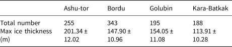
The individually modelled ice thicknesses, obtained by the three models with the same set of measurements for calibration, varied substantially (Fig. 12). Only in the areas with RES measurements, where the ice thickness models are constrained strongly, the individual results matched closely. Generally, differences between the modelled ice thickness increase further away from the RES measurements. For Ashu-Tor and for Golubin glaciers, for instance, modelled ice thicknesses differ considerably with measurement differences up to 100 m. This is mainly caused by the yield stress model which produces much thicker ice (>50–100 m thicker) in the upper part of the glaciers (especially in the accumulation areas). The modelled ice thicknesses of Golubin glacier using the GlabTop model resulted likewise in thicker ice (Bolch, Reference Bolch2015). This can be explained by the very small local slope in this area (Li and others, Reference Li, Ng, Li, Qin and Cheng2012). Moreover, a dominant source of uncertainty for the yield stress model is the absence of RES measurements in the accumulation areas. The RES measurements were, (almost) all, performed in crevasse-free, flat and thus thicker glacier parts associated with compressing flow. This might cause a bias towards higher thickness values where the ice is mainly diverging (Frey and others, Reference Frey, Haeberli, Linsbauer, Huggel and Paul2010). A solution would be to let the ascribed yield stress vary (increase or decrease) towards particular areas as was done in Zekollari and others (Reference Zekollari, Huybrechts, Fürst, Rybak and Eisen2013). Concerning Bordu and Kara-Batkak glaciers, on the other hand, the mass flux 2D model calculates thicker ice, especially along the margins of the glaciers and in the accumulation areas. This can directly be attributed to the larger ice flux in the steeper areas where the plastic flow assumption in the yield stress model reduces the estimated ice thickness (Fig. 12). In addition, only the mass flux 2D model calibrates the flow parameter which might be an important issue for polythermal glaciers (Farinotti and others, Reference Farinotti2017).
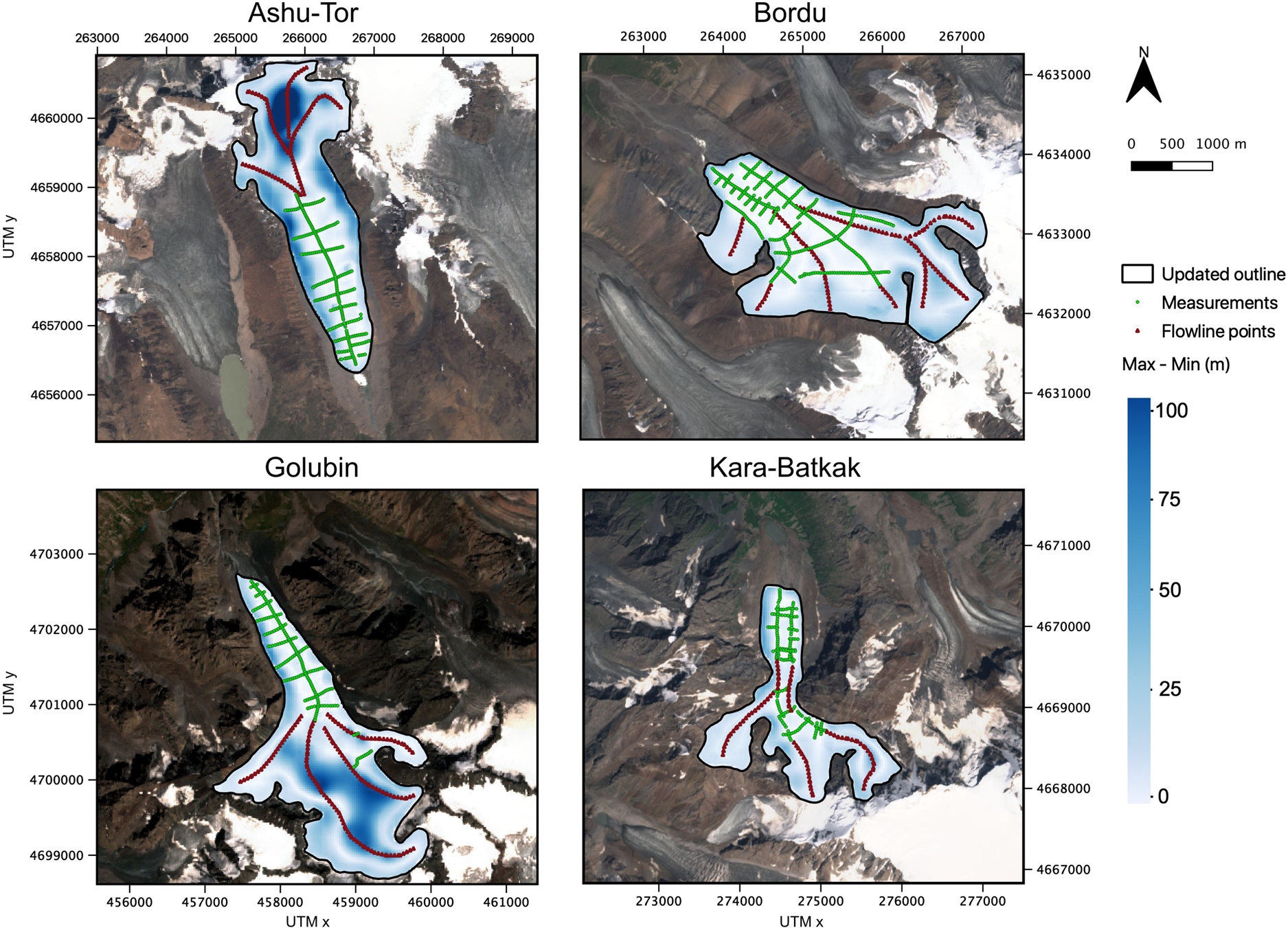
Fig. 12. Difference between the maximum and the minimum modelled ice thickness from all three calibrated models.
The mass flux models’ main uncertainty is introduced by the calculation of the AMB. Both models use dh/dt rates derived from DEM differences and linear SMB gradients derived from individual SMB measurements. Nevertheless, SMB gradients appear to often have a more complex character, especially in the accumulation areas. The inconsistencies that may arise between the dh/dt fields and SMB depending solely on elevation might substantially have influenced the derived AMB. However, it was found by Farinotti and others (Reference Farinotti, Huss, Bauder, Funk and Truffer2009) and Helfricht and others (Reference Helfricht, Huss, Fischer and Otto2019) that the final result of this approach is not very sensitive to changes in the AMB.
6.2 Ice thickness estimates without in situ data
In general, the ice volumes obtained using the volume–area scaling formulas (Macheret and others, Reference Macheret, Cherkasov and Bobrova1988; Bahr and others, Reference Bahr, Meier and Peckham1997; Grinsted, Reference Grinsted2013) and the consensus estimate of Farinotti and others (Reference Farinotti2019) match closely to the ice volumes of the composite ice thickness distributions and to the observations of the ITMIX experiment (Farinotti and others, Reference Farinotti2017). However, our results reveal larger differences concerning local ice thicknesses. We found for instance that the published estimates reconstructed without in situ data all underestimate the maximum ice thickness of Ashu-Tor glacier significantly (>25%). Although this seems very high, it is still within the bounds of 30% which is often cited for maximum local ice thickness error (Huss and Farinotti, Reference Huss and Farinotti2012; Helfricht and others, Reference Helfricht, Huss, Fischer and Otto2019). We also noticed a smaller spread between the different estimates and our measurements for Ashu-Tor and Golubin glaciers compared to Kara-Batkak and Bordu glaciers. This suggests a lower dependency on the model type to estimate the ice thickness of these glaciers (Fig. 10). A similar finding could be noticed in Figure 6. Therefore, the performance of ice thickness models, applied with or without the use of in situ data, appears to depend strongly on the glacier size, type and characteristics. While Ashu-Tor glacier is a typical glacier tongue and rather flat (and differences between the modelled ice thicknesses are smaller), the shape of Kara-Batkak glacier is much more complex (and differences are much larger). Concerning the different estimates, our results revealed that the model of Huss and Farinotti (Reference Huss and Farinotti2012) matches more closely to the measured ice thicknesses compared to the consensus estimate. Hence, it might be preferable to use this model to estimate the ice thickness for unmeasured glaciers in our study area. Models 3 and 4 appeared to match less closely to the measurements. However, model 4 (Fürst and others, Reference Fürst2017), calibrated by the ice thickness measurements (corresponding to the mass flux 2D model in this paper) performed significantly better. This highlights strongly the necessity of in situ data for model calibration and associated model performance.
7. Conclusion
The goal of this research was to obtain an accurate and highly detailed ice thickness distribution of Ashu-Tor, Bordu, Golubin and Kara-Batkak glaciers in the Kyrgyz Tien Shan mountains, which can be used for glacier modelling and to assess water storage. Multiple field campaigns were performed to measure the ice thickness of the glaciers with a RES system. The thickest ice was measured on Ashu-Tor with a maximum of 201 ± 12 m. However, limited accessibility in particular areas of the glaciers, due to crevasses, ice falls and snow cover, hindered full coverage with RES measurements. Hence, three different ice thickness models (yield stress model, mass flux flowline model, mass flux 2D model), calibrated with the measurements, were applied to obtain the ice thickness in the unmeasured areas. Since the modelled ice thicknesses differed considerably and no preferred method could be determined for all four glaciers, a weighted average was assembled to obtain a composite ice thickness distribution. The weights were derived from a performance assessment using a cross-correlation approach between modelled and measured ice thicknesses for a subset of the measurements. For all glaciers, we found that the mass flux 2D model (Fürst and others, Reference Fürst2017) had the lowest errors. Consequently, this model was given the largest weight. A comparison of the ice thickness fields derived in this paper with estimates produced without any in situ data revealed that these estimates approach the total ice volume well but exhibit significant deviations at the local scale. This leads us to conclude that accurate measurements remain necessary for detailed analyses and models. For more general purposes and to assess ice volume, however, estimates of glacier ice thickness without in situ data seem to have sufficient quality in the study area.
Data
All the ice thickness measurements will be submitted to the GlaThiDa (https://www.gtn-g.ch/glathida/) to allow the glaciological community to use the in situ data to optimize the ice thickness models in Central Asia. The adjusted outlines of the glaciers, the DEMs and all the other input data will be provided on request by the first author.
Acknowledgements
We thank Erlan Azisov from the Central Asian Institute of Applied Geosciences (CAIAG) and Martina Barandun from Université de Fribourg for providing the SMB data of Golubin glacier. O.R. was supported by the RFBR grant No. 20-05-00681. Results produced by J.J.F. are based on numerical simulations conducted at the high-performance computing centre of the Regionales Rechenzentrum Erlangen (RRZE) of the University of Erlangen-Nürnberg. Lander Van Tricht holds a PhD fellowship of the Research Foundation-Flanders (FWO-Vlaanderen).


 Open access