


1. Introduction
Imagine that, on a sunny summer day, you go with some friends to the beach. You want to take your sandals off and walk barefoot, but you do not want to burn your feet if the sand is hot, so you ask your friend who has gone ahead: “How’s the sand?” “It’s warm”, they say. You understand them to mean that the sand is only warm, not hot, so you take off your sandals. This reasoning follows from the alternative answer your friend could have given – “It’s hot” – using an informationally stronger alterative to warm. Because they chose not to use this alternative, and because you assume that your friend is cooperative, you reason that their not using the alternative means that they intend to express that it does not hold and, thus, that the sand is warm but not hot (e.g., Geurts, Reference Geurts2010; Grice, Reference Grice1989; Horn, Reference Horn1972; Matsumoto, Reference Matsumoto1995).
The inference from warm to warm but not hot is an example of a scalar inference (SI). To describe SIs, it is often assumed that words like warm are associated with lexical scales consisting of words that are ordered in terms of logical strength, e.g., the scale written as ⟨warm, hot⟩. Lexical scales can consist of adjectives, but also other parts of speech, such as quantifiers ⟨some, all⟩, conjunctions ⟨or, and⟩, nouns ⟨mammal, dog⟩, and verbs ⟨try, succeed⟩ (Hirschberg, Reference Hirschberg1985; Horn, Reference Horn1989). Given a lexical scale of the form ⟨α, β⟩, uttering a sentence containing α in an unembedded position may imply that the corresponding sentence with β is false.
Here, “may imply” is the crucial point, since SI rates vary dramatically across different scales (Doran, Baker, McNabb, Larson, & Ward, Reference Doran, Baker, McNabb, Larson and Ward2009; Gotzner, Solt, & Benz, Reference Gotzner, Solt and Benz2018; van Tiel, Pankratz, & Sun, Reference van Tiel, Pankratz and Sun2019; van Tiel, van Miltenburg, Zevakhina, & Geurts, Reference van Tiel, van Miltenburg, Zevakhina and Geurts2016). To illustrate this scalar diversity, van Tiel et al. (Reference van Tiel, van Miltenburg, Zevakhina and Geurts2016) presented participants with short vignettes in which a character uttered a simple sentence containing the weaker scalar word. Participants were asked if they would infer from this that the character thinks the corresponding sentence with the stronger scalar word was false.
An example of a scale with a low SI rate in van Tiel et al.’s (Reference van Tiel, van Miltenburg, Zevakhina and Geurts2016) experiment is ⟨content, happy⟩. Intuitively, when your friend on the beach tells you “I am content”, you may not immediately infer that they are not happy. In line with this intuition, participants accepted the inference from content to not happy only 4% of the time. Conversely, the SIs of scales like ⟨cheap, free⟩ were extremely robust. Thus, when your friend tells you “The ice creams are cheap”, you are likely to infer that they are not free. Correspondingly, almost all participants in van Tiel et al.’s experiments accepted the inference from cheap to not free.
Again and again, research in recent years has replicated this finding of scalar diversity for the 43 scalar terms that van Tiel et al. (Reference van Tiel, van Miltenburg, Zevakhina and Geurts2016) tested and beyond, and a great deal of work has gone into discovering what factors determine this variability. Operationalising these various factors has generally relied on crowd-sourced ratings (e.g., Gotzner et al., Reference Gotzner, Solt and Benz2018; Sun, Tian, & Breheny, Reference Sun, Tian and Breheny2018) and researcher intuition (e.g., Gotzner et al., Reference Gotzner, Solt and Benz2018). In the current paper, we move away from these judgment-based operationalisations by introducing novel usage-based ways of approximating several factors that are known to affect SI rate, reducing subjectivity in annotation.
In addition to these new operationalisations, this paper also introduces one new factor that predicts scalar diversity: relevance. In particular, we argue that participants are more likely to derive an SI if that SI is generally relevant for the participant upon encountering the weak adjective. Recall the differing SI rates of the scales ⟨content, happy⟩ and ⟨cheap, free⟩. We will argue that part of the reason for this difference is that the SI that enriches the meaning of cheap to cheap but not free is, in general, more relevant than the SI from content to content but not happy.
In this paper, we propose a new, usage-based operationalisation of this general notion of relevance. We test its role in shaping scalar diversity, and we show in two experiments that relevance is a strong predictor of SI rate on top of the factors of semantic distance, polarity, boundedness, and extremeness tested by Gotzner et al. (Reference Gotzner, Solt and Benz2018).
Our first experiment tests these five factors on the data from Gotzner et al.’s (Reference Gotzner, Solt and Benz2018) study using their original operationalisations. Our second experiment tests the same five factors with our novel operationalisations on a new sample of scales, largely replicating the original findings. Like Gotzner et al., we focus on testing adjectival scalar words. Adjectives show a great deal of variety in their SI rates (van Tiel et al., Reference van Tiel, van Miltenburg, Zevakhina and Geurts2016), making them a particularly promising class to study if our goal is to understand scalar diversity.
Unlike Gotzner et al. (Reference Gotzner, Solt and Benz2018), though, and indeed in contrast to much of the literature on SIs, we adopt a rather permissive view of what can be a scale. This is because here we are interested in looking at words that are actually used in a scalar way, rather than those that adhere to strict semantic tests like asymmetric entailment (Horn, Reference Horn1972). Traditionally, many theorists have assumed essentially two types of scales: those that are “in some sense, ‘given to us’” (Gazdar, Reference Gazdar1979, p. 58) and those “where a given context establishes the pragmatic implications on which the scale is based” (Horn, Reference Horn1989, p. 240). The former category of scales includes canonical scales like ⟨warm, hot⟩ and ⟨pretty, beautiful⟩. The latter category ranges from partially ordered sets like ⟨private, corporal, sergeant⟩ (Hirschberg, Reference Hirschberg1985, pp. 97–98) to truly context-dependent, ad-hoc scales like ⟨back, well and back⟩ in (1), from Gazdar (Reference Gazdar1979, p. 51).
In this paper, we assume that lexical scales arise whenever the inference from the weaker scalemate to the negation of the stronger one is relevant. This permissive view takes the two types of scales mentioned above as its limiting cases: in the case of given scales, the inference is relevant in almost any context; in the case of ad-hoc scales, the inference is only relevant in very specific contexts.
We begin in Section 1.1 by recounting what is already known about how the already-established factors of polarity, semantic distance, boundedness, and extremeness influence SI rate, and introducing our novel operationalisations of each of them. We then move on to the concept of relevance and show how it can be approximated using corpus data. Specifically, we look at how frequently scalar adjectives are used in corpora in what we term “scalar constructions”, such as α but not β. The basic idea here is that the more frequently scalar adjectives are used in these constructions, the more relevant the SI becomes, since an explicit contrast between weak and strong adjectives is encountered more often. Thus, it is more likely that the SI will be derived when the weak word is used in isolation. Section 1.2 will discuss this idea in more detail. Then, Section 1.3 outlines our procedure for identifying scalar constructions from the ENCOW16A web corpus (Schäfer, Reference Schäfer, Bański, Biber, Breiteneder, Kupietz, Lüngen and Witt2015; Schäfer & Bildhauer, Reference Schäfer, Bildhauer, Calzolari, Choukri, Declerck, Doğan, Maegaard, Mariani, Moreno, Odijk and Piperidis2012).
The assumption implicit in using data from any corpus as a proxy for language exposure is that the language that people are likely to experience is approximated by the texts contained in the corpus. For this reason, we are using the very large, very diverse corpus ENCOW16A. Since it contains 16.8 billion tokens of English from web texts encompassing an enormous range of genres and registers, it is a good approximation of the linguistic input that people in the English-speaking world are likely to face.
Following this exposition, we turn to our two experiments. Experiment 1 in Section 2 tests the five factors – relevance, polarity, semantic distance, boundedness, and extremeness – on SI rate data gathered by Gotzner et al. (Reference Gotzner, Solt and Benz2018). One of the limitations of the current experimental record is that the tested scales were always hand-picked by researchers: another subjective procedure that results in potentially idiosyncratic scales being tested and also overlooks the question of which scales people are actually familiar with based on use. Hence, Experiment 2 in Section 3 replicates the results of Experiment 1 (using our new operationalisations of Gotzner et al.’s original predictors) on a systematically selected sample of fifty adjectival scales identified from ENCOW16A.
Section 4 considers what insights we can gain from these results for our new operationalisations, explores how our measure of relevance is related to the notion of questions under discussion, and addresses the hitherto underexplored relationship between usage, cognition, and pragmatic reasoning. Finally, Section 5 concludes with speculations on our proposal’s generalisability and perspectives for future research.
1.1. new operationalisations of factors affecting SI rate
This section outlines four factors that have been previously shown to affect SI rate and presents our methods for operationalising them. As stated above, we move away from using crowdsourcing and researchers’ intuitions to classify and describe adjectives, and toward operationalising these measures with computational tools based on empirical usage data from corpora. This method allows us to overcome the subjectivity inherent in language users’ intuitions by grounding these judgments in objective data from language use. Moreover, some of the measures used to predict scalar diversity appeal to complex notions such as semantic distance or polarity, and it is not always clear whether we succeed in making lay participants grasp these concepts in experimental tasks. By deriving predictors from usage data, our approach avoids these potential pitfalls and allows the synthesis of multiple, potentially conflicting, measures of the same abstract concept (van Tiel & Pankratz, Reference van Tiel and Pankratz2021).
It should be noted that our goal in the present paper is not to apply all predictors that the literature has found to significantly predict SI rate; our more modest aim is to concentrate on the four factors tested by Gotzner et al. (Reference Gotzner, Solt and Benz2018). Further factors with great explanatory power have also been uncovered (e.g., local enrichability by Sun et al., Reference Sun, Tian and Breheny2018, and semantic similarity of scalemates by Westera & Boleda, Reference Westera and Boleda2020), but we believe that the synthesis of all predictors of scalar diversity is best left for future work.
1.1.1 Polarity of the scale
Polarity concerns whether a scale is positive like ⟨good, great⟩ or negative like ⟨bad, awful⟩ (words on a lexical scale always share the same polarity; Fauconnier, Reference Fauconnier1975; Horn, Reference Horn1989). Negative scales tend to yield higher SI rates than positive ones, which may be because each type of scale involves different presuppositions (Cruse, Reference Cruse1986; Gotzner et al., Reference Gotzner, Solt and Benz2018; Rett, Reference Rett2008). Specifically, positive scalar terms suggest that the entire underlying dimension is relevant, whereas negative terms tend to restrict the range of possible interpretations to those occurring on the negative part of that dimension. Hence, How good was it? is compatible with both positive and negative answers, whereas How bad was it? presupposes that it was bad to some degree. Gotzner et al. (Reference Gotzner, Solt and Benz2018) suggest that, since negative scalar words are generally associated with a narrower part of the underlying dimension, they are more strongly associated with their scalemates, which may lead to elevated SI rates.
However, as those authors observe, adjectival polarity is difficult to annotate, since the notion of polarity is highly multifaceted. Diagnostics of its different aspects exist, ranging from the presence of morphological negative marking to intuitive emotional valence (Ruytenbeek, Verheyen, & Spector, Reference Ruytenbeek, Verheyen and Spector2017), but these often point in contradictory directions (Gotzner et al., Reference Gotzner, Solt and Benz2018, p. 7). Here, we unify two diagnostics of polarity by using a continuous measure obtained using principal component analysis (PCA), along the lines of van Tiel and Pankratz (Reference van Tiel and Pankratz2021).
The first diagnostic is emotional valence, based on the scores from Mohammad’s (Reference Mohammad2018) Valence, Arousal, and Dominance Lexicon. Mohammad collected these scores by first presenting annotators with four words and asking them to select the most positive and the most negative word from those four. Then, these choices were aggregated into a single valence score per word by taking the proportion of times the word was selected as the most positive and subtracting the proportion of times the word was selected as the most negative (pp. 176–177).
The second diagnostic is the adjective’s compatibility with ratio phrases like twice as (Sassoon, Reference Sassoon2010). This diagnostic separates positive and negative adjectives because such ratio phrases presuppose a natural zero point, and while positive adjectives generally have one, negative adjectives do not. To illustrate: twice as tall is fine, while twice as short is odd, since there is no natural zero point for shortness. For this diagnostic, we use the number of times that each adjective occurs following twice as in the ENCOW16A web corpus, scaled by the adjective’s absolute frequency.
We synthesise these two different ways of measuring polarity—one intuitive, one usage-based—into a single continuous variable by applying PCA. PCA summarises the information contained in a multivariate dataset using new variables called principal components. Principal components are linear combinations of the original variables, and they can be understood as new axes being drawn through the dataset’s original space. The first principal component (PC1) is drawn through this space in such a way that it accounts for the largest possible amount of the variance in the dataset, extracting as much information as possible. In the data for Experiment 1, PC1 accounts for 52% of the variance, and in Experiment 2, 56%. Our measure of polarity consists of the projections onto PC1 of the data points for valence and co-occurrence with twice as. We expect the SI rate to decrease as polarity increases.
1.1.2. Semantic distance between scalemates
Consider the sentences in (2). Van Tiel et al. (Reference van Tiel, van Miltenburg, Zevakhina and Geurts2016, p. 160) observe that an utterance of (2a) is more likely to imply the negation of (2c) than it is to imply the negation of (2b).

Van Tiel et al. (Reference van Tiel, van Miltenburg, Zevakhina and Geurts2016) connect this observation to the notion of semantic distance. The semantic distance between two words indicates how easy it is to distinguish their meanings. In the case at hand, the semantic distance between many and all is greater than between many and most, i.e., it is easier to determine whether many or all of the senators voted against the bill than whether many or most of them did. More generally, the greater the semantic distance between two scalemates, the more robust the SI (see also the discussion in Horn, Reference Horn1972, p. 112).
To understand the relevance of semantic distance, it is important to acknowledge that the derivation of SIs is a two-step process (e.g., Sauerland, Reference Sauerland2004). Thus, an utterance of (2a) first gives rise to a weak inference, or ignorance implicature, according to which the addresser was not in a position to say either (2b) or (2c). (We use the terms ‘addresser’ and ‘addressee’ throughout as an alternative to the spoken-language-biased ‘speaker’ and ‘hearer’.) These weak inferences may then be strengthened to a proper SI according to which the addresser believes the alternatives to be false. Importantly, the validity of this inferential step depends on whether the addresser is competent, i.e., knows whether the alternatives are true or false.
Intuitively, there is a close connection between semantic distance and the plausibility of the competence assumption, such that if the meanings of two words can easily be distinguished (i.e., if they have a large semantic distance), the competence assumption is a priori more plausible. This connection would then explain why greater semantic distance is associated with higher rates of SI.
Semantic distance between scalemates has indeed been shown to be a significant predictor of SI rate. Van Tiel et al. (Reference van Tiel, van Miltenburg, Zevakhina and Geurts2016, p. 163) find that greater semantic distance leads to a greater likelihood of SI computation across many different types of scales, and Gotzner et al. (Reference Gotzner, Solt and Benz2018, p. 10) replicate the finding on exclusively adjectival scales (see also Beltrama & Xiang, Reference Beltrama and Xiang2013). Van Tiel et al. (Reference van Tiel, van Miltenburg, Zevakhina and Geurts2016, p. 162) and Gotzner et al. (Reference Gotzner, Solt and Benz2018, p. 6) measured semantic distance based on participants’ judgments on a seven-point Likert scale. Participants were asked how much stronger a statement containing the stronger scalemate was, compared to an otherwise identical statement containing the weaker scalemate.
In Experiment 1, we use the semantic distance judgments from Gotzner et al. (Reference Gotzner, Solt and Benz2018). In Experiment 2, however, we operationalise semantic distance using word embeddings (see also Soler & Apidianaki, Reference Soler and Apidianaki2020; Westera & Boleda, Reference Westera and Boleda2020). Word embeddings are a computational tool, a way of representing word meanings numerically based on the so-called ‘distributional hypothesis’: the idea that words with similar meanings tend to be used in similar linguistic environments (Firth, Reference Firth and Palmer1957). Embeddings represent word meanings as the environments that that word tends to occur in, encoded as a numeric vector (Jurafsky & Martin, Reference Jurafsky and Martin2020, p. 96).
Thinking of word meanings as vectors, we can represent the difference in meaning between two words as the difference of the two corresponding vectors. Thus, we compute the vector differences between 300-dimensional Word2Vec embeddings pre-trained on the Google News corpus (Mikolov, Chen, Corrado, & Dean, Reference Mikolov, Chen, Corrado and Dean2013) via the gensim library for Python (Řehůřek & Sojka, Reference Řehůřek and Sojka2010). The difference between two vectors is still 300-dimensional, but we want a single scalar value for each adjective pair that represents their difference to serve as a predictor in the statistical analysis. Therefore, we again perform PCA and use PC1 as a summary of the vector differences between scalemates. Although PC1 only explains 6% of the variance in the difference vectors, it is positively correlated with the semantic distance ratings of Gotzner et al. (Reference Gotzner, Solt and Benz2018), indicating its adequacy as an approximation of semantic distance. We expect SI rate to increase as semantic distance increases.
1.1.3. Boundedness of the scale
Boundedness is a characteristic of scales determined by the stronger scalemate. Specifically, a scale is bounded if the stronger scalemate denotes an endpoint on the scale, rather than a more extreme but still non-terminal interval (van Tiel et al., Reference van Tiel, van Miltenburg, Zevakhina and Geurts2016, p. 163). For example, boundedness is the difference between the scales ⟨good, great⟩ (unbounded) and ⟨good, perfect⟩ (bounded); there’s room for improvement beyond great, but nothing can be better than perfect.
The role of boundedness for computing SIs goes back to Horn (Reference Horn1972, p. 112), who stated that bounded scales deterministically trigger SIs, while unbounded scales may or may not. Although not to this extent, bounded scales do consistently show higher SI rates than unbounded ones (van Tiel et al., Reference van Tiel, van Miltenburg, Zevakhina and Geurts2016, p. 164; Gotzner et al., Reference Gotzner, Solt and Benz2018, p. 7). The reason that boundedness plays a role is presumably similar to the role of semantic distance. For instance, it may be easier to determine, say, whether something is good or perfect than to determine whether something is good or great. Hence, someone interpreting “It is good” is more secure when concluding that it is not perfect than that it is not great.
An adjective’s status as a scalar endpoint can be evaluated based on its compatibility with so-called totality modifiers like completely, absolutely, and almost (Paradis, Reference Paradis2001, p. 49; Gotzner et al., Reference Gotzner, Solt and Benz2018, p. 7). These modifiers are felicitous with scalar endpoints (e.g., completely perfect, almost perfect), but sound odd or coerce a terminal-like interpretation with non-terminal intervals (e.g., ?completely great, ?almost great).
Rather than relying on intuitive judgments of felicity, we use a supervised machine learning algorithm – specifically, a random forest (Breiman, Reference Breiman2001) – to classify scales based on the frequency in ENCOW16A of the strong adjective following 72 different modifiers. Among these are the totality modifiers from Paradis (Reference Paradis2001), as well as synonyms like totally and perfectly (these make up 13 of the 72 modifiers). The selection also includes 27 modifiers that indicate that an adjective is not a scalar endpoint, but instead gradable – i.e., denoting a degree of some potentially abstract measurement (Kennedy, Reference Kennedy2007, p. 4) – such as slightly, very, and relatively. The reason for including these is that, just as high frequency with totality modifiers indicates that an adjective is a scalar endpoint, high frequency with gradability modifiers indicates that it is not. Additionally, 21 modifiers were included that do not fit cleanly into either category (e.g., truly) or are evaluative in nature (e.g., wonderfully), in order to give the classifier more data to work with. What the remaining eleven modifiers are will be explained in the next section. It should be noted that the exact nature of the modifiers is not important for the classifier, since it does not use any categorisation of modifiers into different types, but merely focuses on their frequencies with bounded vs. unbounded strong adjectives.
Using Gotzner et al.’s (Reference Gotzner, Solt and Benz2018) annotations of boundedness as a gold standard, we trained a random forest classifier on their data using the Python library scikit-learn (Pedregosa et al., Reference Pedregosa, Varoquaux, Gramfort, Michel, Thirion, Grisel, Blondel, Prettenhofer, Weiss, Dubourg, Vanderplas, Passos, Cournapeau, Brucher, Perrot and Duchesnay2011). A random forest classifier consists of many decision tree classifiers. A decision tree classifier creates a tree structure in which the internal nodes are features (one of the 72 modifiers) with some threshold frequency value and, in our case, two branches coming off each. The leaf nodes are the classes to be assigned (bounded vs. unbounded). The feature and threshold that optimally divide the data are chosen at each step. An example decision tree is shown in Figure 1.

Fig. 1. An example decision tree classifier for boundedness (non-natural values indicate that the classifier placed the threshold between two frequency values).
The benefit of a random forest over a single decision tree is that, by combining many trees and training each on a random subset of the full dataset, the model becomes more robust to noise in the data and reaches higher predictive accuracy (Breiman, Reference Breiman2001, p. 5). In short, the classifier guesses based on the frequency of each strong adjective with each modifier whether the strong adjective is a scalar endpoint or not. We used a 70/30 training/testing split, and the resulting classifier had an accuracy of 85% on the held-out test items. In line with previous findings, we expect bounded scales to have a higher SI rate than unbounded ones.
1.1.4. Extremeness of the strong adjective
The class of extreme adjectives contains expressions like excellent, huge, and gorgeous: adjectives that denote an extreme interval on their respective dimensions (see, e.g., Beltrama & Xiang, Reference Beltrama and Xiang2013; Cruse, Reference Cruse1986; Gotzner et al., Reference Gotzner, Solt and Benz2018; Morzycki, Reference Morzycki2012; Paradis, Reference Paradis2001). This class of adjectives can be identified by their compatibility with so-called ‘extreme degree modifiers’ (Beltrama & Xiang, Reference Beltrama and Xiang2013, p. 85; Morzycki, Reference Morzycki2012, p. 568) like downright, positively, and flat-out (e.g., downright huge vs. ?downright big, showing that huge is an extreme adjective, but big is not).
Based on the reasoning we have already seen for semantic distance and boundedness, we would expect a higher SI rate for scales with extreme adjectives as the stronger scalemate; it is easier to determine whether something is warm vs. searing (extreme) than it is to determine whether something is warm vs. hot (non-extreme). However, Gotzner et al. (Reference Gotzner, Solt and Benz2018) found the opposite: scales with extreme adjectives as stronger members had lower SI rates than those with non-extreme stronger scalemates. They explain these results by proposing that, since extreme adjectives have considerably different conditions of use than their non-extreme scalemates, they may not arise as alternatives for the purposes of SI computation.
We trained another random forest classifier to predict whether a strong adjective is extreme or non-extreme based on its frequency with the same set of 72 modifiers described above. In addition to the shibboleth modifiers for boundedness and gradability mentioned above, this set also contains the eleven extreme degree modifiers put forward by Morzycki (Reference Morzycki2012). The classifier was again trained using Gotzner et al.’s (Reference Gotzner, Solt and Benz2018) annotations of extremeness as a gold standard with a 70/30 training/testing split, and it also showed an accuracy of 85% on the held-out test items. Because theory and the previous experimental record are at odds about the effect of extremeness on SI rate, we have no clear predictions concerning the hypothesised direction of the effect.
1.2. relevance
We now turn to a factor that is intuitively important for scalar diversity but that has not yet been studied in depth in this context: relevance. In addition to the four factors outlined above, whether an SI is drawn is also affected by the context in which an utterance takes place. If the context makes the SI relevant, the SI is more likely to be computed (Geurts, Reference Geurts2010; Matsumoto, Reference Matsumoto1995; McNally, Reference McNally, Ostrove, Kramer and Sabbagh2017; Ronai & Xiang, Reference Ronai and Xiang2020). Consider the beach scene described at the beginning of this paper. Since the difference between the sand being warm vs. hot is the difference between your feet being safe vs. burned, the difference between warm and hot (and in particular the negation of hot, i.e., the SI) is relevant in this context (McNally, Reference McNally, Ostrove, Kramer and Sabbagh2017, pp. 23–24). On the other hand, if you book a holiday to get out of the cold, you may not care whether your destination is hot or just warm. In this way, different contexts can change the relevance of the SI. And we argue that by generalising over the different contexts in which scalar words are used, we may arrive at a measure of general relevance for each SI. Although relevance has long been discussed in the literature (for example by Cummins & Rohde, Reference Cummins and Rohde2015; Zondervan, Reference Zondervan2010), it has (to our knowledge) not yet been operationalised and explicitly tested as a predictor of scalar diversity. Here, we propose a way to do this.
Our basic hypothesis is as follows. First, we assume that SIs have some measure that indicates their general relevance (i.e., relevance even in the absence of a situated context, learned as a sort of default over repeated exposure to scalar words in use). If the SI is relevant, then in language use people will be more likely to delineate the weaker term from a stronger scalemate. By ‘delineate’, we mean using the weaker term in such a way that its meaning excludes that of the stronger scalemate. One way they might do this is by producing an SI, but luckily – since the frequency of SIs in everyday language use is difficult, if not impossible, to determine – this is not the only way. Another possibility for observing how frequently people explicitly draw a line between the weaker and stronger scalar words is how they use these words in scalar constructions.
Scalar constructions are patterns such as α but not β and α, even β (where α represents the weaker adjective, and β the stronger one). Usage in scalar constructions indicates both a scalar relationship and a categorical distinction between the two scalemates involved (de Melo & Bansal, Reference de Melo and Bansal2013; Horn, Reference Horn1972; Sheinman & Tokunaga, Reference Sheinman and Tokunaga2009; van Miltenburg, Reference van Miltenburg2015; Wilkinson, Reference Wilkinson2017). If adjectives from the same scale frequently co-occur in scalar constructions, then repeated exposure to this pattern will continually reinforce the scalar relationship as well as the conceptual delineation between them. Then, because of the accumulated exposure to this meaning in the scalar construction, experiencing the weak adjective alone may be enough to trigger the meaning that includes an upper bound, i.e., the implicature-enriched meaning.
We believe that the expectation that relevance is reflected in usage in this way is a reasonable one. Usage-based theories have long established, on the one hand, that “usage patterns, frequency of occurrence, variation, and change … provide direct evidence about cognitive representation” (Bybee & Beckner, Reference Bybee, Beckner, Heine and Narrog2009, p. 827), and on the other hand, that language structure emerges out of humans’ experiences with language (Bybee & Beckner, Reference Bybee, Beckner, Heine and Narrog2009; Diessel, Reference Diessel and Aronoff2017; Goldberg, Reference Goldberg2006; Gries & Ellis, Reference Gries and Ellis2015; Tomasello, Reference Tomasello2003). Thus, the more that we experience linguistic elements in particular contexts with particular conjunctions of features, the more these contexts influence how we perceive the elements individually (Goldberg, Reference Goldberg2006, p. 14; Gries & Ellis, Reference Gries and Ellis2015, pp. 230–231). And much evidence also speaks for cumulative, long-term histories of exposures to words shaping the way people use them (Bybee, Reference Bybee2002; Raymond, Brown, & Healy, Reference Raymond, Brown and Healy2016).
Therefore, it is probable that a priori relevance influences the way that scalar adjectives are used, but also that their usage further reinforces cognitive representations of relevance. Thus, usage and cognitive representations conspire to make the SI relevant, and this relevance should be reflected in SI rates. Van Tiel et al. (Reference van Tiel, van Miltenburg, Zevakhina and Geurts2016, p. 168) also allude to this idea, mentioning that scales might behave idiosyncratically because people are “alert to all manner of statistical patterns in language use”, such as “the frequency with which scalar expressions give rise to upper-bounded interpretations”.
One of our reviewers mentioned that, in principle, an alternative hypothesis would also be possible, namely that what is left unsaid when making implicatures should also be left unsaid in corpus data. In concrete terms, imagine that a weaker scalar term α reliably leads to an SI. Then, it would not be necessary to explicitly spell out this SI in scalar constructions like α but not β. The corpus would then contain fewer instances of α but not β if α robustly licenses an SI. The result would be a negative association between the two measures, rather than the positive one we predict.
Another slightly different alternative could also be derivable from a usage-based account: from frequent exposure to the scalar construction α but not β, say, people may derive that the added but not β is required for α to have an upper-bounded meaning. The lack of an explicit rejection of β would then lead to fewer SIs when α is used on its own. This is also the opposite of what our account predicts.
What both of these hypotheses presuppose, though, is that the SI-enriched, upper-bounded meaning of α and the explicit statement of α but not β are always functionally equivalent and interchangeable. Otherwise, what motivation would there be for the first alternative hypothesis to expect that the SI fills the same role as explicit statement of but not β, or for the second alternative to infer the unenriched meaning from an absent but not β?
For all their commonalities, though, we know that the inferred negation of the stronger term in SIs and the explicit negation of the alternative differ in several ways. For one, the enriched meaning in the SI is cancellable (e.g., I ate some of the cookies; in fact, I ate all of them), unlike literal negation. Further, including an explicit negation of the alternative also changes the argumentative direction of the statement containing the scalar term (Ariel, Reference Ariel2020). Consider the example in (3): while most is appropriate in (3a), most but not all is odd in sentence (3b), since it changes the argumentative direction of the statement.
The alternative hypotheses overlook the differences between the inferred upper-bounded meaning and the explicit one, and are thus, in our opinion, less plausible than the hypothesis we put forward here.
How can this notion of general relevance that we assume be operationalised? We propose that it can be approximated as the token frequency of co-occurrences of the weak adjective with a stronger scalemate in scalar constructions. The more frequently a weak adjective is encountered in an explicitly scalar relationship with some stronger scalemate, the more the scalar relationship on the one hand and the delineation between the two concepts on the other hand will be driven home. We use tokens rather than types because “every token of use impacts cognitive representation” (Bybee & Beckner, Reference Bybee, Beckner, Heine and Narrog2009, p. 833).
It should be noted that, in looking at corpus data, we are actually looking at a large collection of individual contexts and learning about the relevance of SIs in these contexts. However, we argue that, by summing over all contexts we find in the corpus, we get an idea of what people tend to talk about, and thus what people tend to consider relevant, and that therefore our measure is a plausible approximation of the general relevance of an SI. In order to compute this measure of relevance, we need a set of scalar constructions within which scalar adjectives may occur. Our procedure for discovering these from ENCOW16A is outlined next.
1.3. Discovering scalar constructions
We follow a method outlined by Hearst (Reference Hearst1992, pp. 3–4) to identify scalar constructions (see similar procedures in Sheinman & Tokunaga, Reference Sheinman and Tokunaga2009, Section 2.1, and de Melo & Bansal, Reference de Melo and Bansal2013, Section 4.1). The first step is to identify pairs of scalar adjectives. The next step is to find environments in a corpus in which those two adjectives occur near one another. Frequent environments are likely to be ones that indicate the relation of interest.
For the first step, we selected six canonical adjectival scales from Horn (Reference Horn1972, p. 47) and Hirschberg (Reference Hirschberg1985, p. 101), and then added two more (the final two in the following list) to better balance the positive and negative scales: ⟨warm, hot⟩, ⟨cool, cold⟩, ⟨pretty, beautiful⟩, ⟨happy, ecstatic⟩, ⟨intelligent, brilliant⟩, ⟨good, excellent⟩, ⟨small, tiny⟩, and ⟨bad, horrible⟩. For each scale, we retrieved all sentences in ENCOW16A that contained both of these scalemates in either order, separated by a window of 1–5 tokens (inclusive). This resulted in 43,929 sentences.
We then applied two templates, corresponding to the regions in which scalar constructions may appear, to each sentence. The first template is [α interfix β], e.g., α but not β. The second is [prefix α interfix β], e.g., very α, even β (but see Sheinman & Tokunaga, Reference Sheinman and Tokunaga2009, who also included a postfix). Infrequent patterns in these regions are likely just noise. We therefore removed the lowest-frequency patterns (those with token frequency <20 for the first template, <5 for the second), and manually coded the remaining ones to remove those that did not clearly evoke a scale (e.g., during α or β, or with α/β). This left us with a list of 25 candidate scalar constructions, shown in the first column of Table 1.
TABLE 1. For each candidate construction, the sum of the co-occurrence counts of each weak adjective with its stronger scalemate and its antonym, and the preference of the construction for the stronger scalemate (+) or the antonym (–)

Hearst’s (Reference Hearst1992) roadmap ends here, but we took one more step, because these 25 candidates still vary in an important way. Some of them seem to prefer housing two scalar terms on opposite ends of the scale, while others prefer terms both at the same end of the scale. We want to keep only the latter type, since these will be more likely to yield true scalemates when we use them to detect scalar pairs (as we will describe in Section 3.1), and ignoring the scales that prefer antonym pairs reduces the amount of data that must be gone through by hand as well as the noise within that data. Therefore, our final elimination phase was essentially a simplified collostruction-style analysis of whether the construction is more likely to contain a stronger scalemate or an antonym (Stefanowitsch & Gries, Reference Stefanowitsch and Gries2003).
To do this, we took three canonical scales – size, quality, and temperature – in positive and negative versions, and in each case identified an antonym (e.g., ⟨warm, hot⟩ has the antonym cold). Then, we counted the occurrences in ENCOW16A when the weak adjective appeared in each construction with its stronger scalemate (e.g., warm but not hot) and with its antonym (e.g., warm but not cold). These values, aggregated by construction, appear in the second and third columns in Table 1. The final column in Table 1 indicates with a + that the frequency of co-occurrence with the stronger scalemate is greater than with the antonym, and the opposite with a −. We excluded all constructions with a negative sign, leaving a final selection of twenty scalar constructions.
Our constructions differ from those in de Melo and Bansal (Reference de Melo and Bansal2013) and Sheinman and Tokunaga (Reference Sheinman and Tokunaga2009) in a noteworthy way. Their constructions include many in which the stronger adjective precedes the weak adjective, e.g., not β, although still α (de Melo & Bansal, Reference de Melo and Bansal2013, p. 280). We found only three constructions with this pattern (the final three rows in Table 1), and they all prefer the antonym over the stronger scalemate. This suggests that, if the goal is to use scalar constructions to automatically detect and order adjectival scalemates (as it is in those two papers), scalar constructions in which the weaker adjective precedes the stronger one will be more informative about the ordering of those terms.
Before turning to the first experiment, we summarise Section 1 in Table 2, which shows the hypothesised effect of each predictor on the rate at which SIs are derived.
TABLE 2. Hypothesised direction of effect of each predictor (the categorical predictors, boundedness and extremeness, are coded with unbounded and non-extreme levels as 0, so a positive sign means that SI rate should be higher for bounded and extreme adjectives)

2. Experiment 1
Our first experiment uses the SI rate data from Gotzner et al. (Reference Gotzner, Solt and Benz2018) for 68 different lexical scales. As mentioned above, Gotzner et al. gathered these SI rates in an experiment based on the paradigm of van Tiel et al. (Reference van Tiel, van Miltenburg, Zevakhina and Geurts2016). Participants read a scenario in which a character makes a statement containing a weak scalar adjective. Then, participants are asked whether they would endorse the corresponding SI, i.e., a sentence containing the negation of the stronger scalemate. For instance, if Mary says “He is intelligent”, participants would be asked “Would you conclude from this that, according to Mary, he is not brilliant?” (Gotzner et al., Reference Gotzner, Solt and Benz2018, p. 6). The range of SI rates obtained by Gotzner et al. (Reference Gotzner, Solt and Benz2018) is visualised in Figure 2 for a subset of the adjectives they tested.

Fig. 2. A sample of the SI rates observed by Gotzner et al. (Reference Gotzner, Solt and Benz2018).
2.1. Computing relevance
To gather the data for our relevance measure – which, recall, requires the token count of stronger scalemates co-occurring in scalar constructions with each weak adjective – we queried ENCOW16A for all adjectives that co-occur with Gotzner et al.’s (Reference Gotzner, Solt and Benz2018) weak adjectives in the 20 scalar constructions identified above. We then tidied the resulting dataset to remove spurious matches, primarily words (and unidentifiable non-words) falsely tagged as adjectives. Unambiguous typos were corrected and kept in the dataset. We removed any cases in which the weak adjective also occurred in the stronger adjective slot, e.g., cool but not cool. Additionally, whenever the word before the strong adjective slot was not, we removed the co-occurring adjective sure, because those were instances of the phrase not sure rather than legitimate scalar constructions.
Further, all six constructions that begin with very, only, and just have corresponding constructions without these initial words. This is important because the query for, e.g., very α, even β returns a proper subset of the result for α, even β. To account for this duplicated data, we removed the repeated entries from the more general construction (e.g., α, even β), maintaining the data only for the more specific construction (e.g., very α, even β), since it is an instance of the latter, not the former.
We then annotated the tidied data, noting whether each co-occurring adjective could be considered a stronger scalemate to the weak adjective. To reduce the subjectivity in this procedure, both authors annotated all adjectives, and only the adjectives that both authors judged to be a stronger scalemate were considered as such in the analysis. Figure 3 illustrates the distribution of co-occurring adjectives for the weak adjective good, which had a fairly high co-occurrence rate with stronger scalemates, and big, which did not.

Fig. 3. Frequency of adjectives co-occurring in the strong adjective slot of scalar constructions with good and big.
2.2. results
Using the package lme4 (Bates, Mächler, Bolker, & Walker, Reference Bates, Mächler, Bolker and Walker2015) in R (R Core Team, 2019), we fit a binomial generalised linear mixed model that predicts Gotzner et al.’s SI rate as a function of relevance, polarity, semantic distance, boundedness, and extremeness, including random intercepts for participants. For fitting the model, the continuous measures of relevance, polarity, and semantic distance were centered. The categorical measures, boundedness and extremeness, were treatment-coded with the unbounded and non-extreme conditions as the baseline, respectively.
The model’s estimates (in log-odds space) are shown in Table 3. This model explains 19% of the variance in the data, with 8% coming from the fixed effects and 11% from the random effects (R 2 values computed using the rsq package; Zhang, Reference Zhang2020). Figure 4 visualises the model’s population-level (fixed effect) predictions of the effects of each of these factors, with all other factors held at their baseline level, back-transformed to the original proportion space.
TABLE 3. Model estimates for predictors of SI rate in Experiment 1


Fig. 4. Population-level model predictions for Experiment 1; ribbons and error bars represent the 95% confidence intervals.
Unsurprisingly, we replicate the findings for semantic distance, polarity, boundedness, and extremeness that Gotzner et al. (Reference Gotzner, Solt and Benz2018) reported. SI rate is significantly higher for semantically more distant scalemates, more negative scales, bounded scales, and scales with a non-extreme strong adjective. We also show that relevance is a significant predictor of SI rate.
2.3. outlook
The results of Experiment 1 encourage the idea that relevance, as approximated by usage, contributes to the probability of computing an SI. However, the materials used were not constructed in a systematic way in terms of frequency, polysemy, and experimental presentation. The next section presents a replication of Experiment 1 with a more empirically motivated selection of adjectives and more carefully designed experimental materials.
3. Experiment 2
Experiment 2 aims to replicate the effect of relevance using a more principled sample of weak adjectives. For one, we focus on high-frequency adjectives. According to a usage-based account, it is for these that the relationship between relevance and SI rate should be most robust, since it will have had the most opportunity to establish itself through repeated exposure. For another, we focus on adjectives with low semantic diversity, i.e., adjectives that are relatively non-polysemous, for reasons that will be discussed in Section 3.1. We sampled 50 adjectival scales, and using these we ran an experiment using a single-trial design with the same SI-endorsement paradigm as in van Tiel et al. (Reference van Tiel, van Miltenburg, Zevakhina and Geurts2016) and Gotzner et al. (Reference Gotzner, Solt and Benz2018) (Section 3.2). The overall results of Experiment 2 will be explored in Section 3.3 .
3.1. Identifying adjectival scales
To arrive at our sample of 50 scales, we iteratively narrowed down a large number of adjectives based on a sequence of criteria, and then used scalar constructions to find the most frequent stronger scalemate in each case. We began with the 1500 most frequent adjectives in ENCOW16A (corresponding to a token frequency of over 46,193). Our first criterion was semantic diversity since, for several reasons, we want to avoid polysemous weak adjectives. The first reason is that, for polysemous adjectives that appear on more than one scale, it is unknown whether the SI rate on one scale may affect the SI rate on another, so we bypass this potential source of noise. Second, avoiding polysemy is a step toward addressing the critique from McNally (Reference McNally, Ostrove, Kramer and Sabbagh2017) that the interpretation of polysemous adjectives depends greatly on situational context, something which is not available in the experimental paradigm used here.
Further, it has been shown that scales with a greater degree of polysemy (as measured by how well two scalemates can be interpreted as not being on the same entailment scale) are associated with lower SI rates (Sun et al., Reference Sun, Tian and Breheny2018). That study also finds that this measure of polysemy is highly correlated with semantic distance ratings (p. 8). Thus, controlling for polysemy factors out its potential effect on SI rate and prevents possible issues of multicollinearity, since, as we have seen, semantic distance is also included in our models.
To find non-polysemous adjectives, we return to the distributional hypothesis. If all contexts that a word appears in are quite similar to one another, then the word likely means the same thing in every instance. In contrast, if the contexts are very diverse, the word is probably being used with several different meanings (Cevoli, Watkins, & Rastle, Reference Cevoli, Watkins and Rastle2021, p. 248; Hoffman, Lambon Ralph, & Rogers, Reference Hoffman, Lambon Ralph and Rogers2013, p. 718). This intuition is captured by the Latent Semantic Analysis method of Hoffman et al. (Reference Hoffman, Lambon Ralph and Rogers2013). We use the weighted, lemmatised semantic diversity scores computed using this method and made available by Cevoli et al. (Reference Cevoli, Watkins and Rastle2021). The scores range between 0 and 1, and we set a threshold such that known polysemous scalar adjectives like hard, low, and high were excluded. This threshold, at the 33rd quantile of the distribution of scores, rejected adjectives with a semantic diversity score over 0.69, narrowing the 1500 adjectives down to 446.
The next criterion looked at scalarity: Which of these adjectives are actually used in a scalar way? For this, we return to the scalar constructions identified above. We inserted each of the 446 adjectives into the weak adjective slot in each construction and queried ENCOW16A for all adjectives appearing in the strong adjective slot. After tidying the data as described above, we discarded any weak adjectives that appear under one hundred times in scalar constructions, interpreting this low frequency as a lack of robust scalar meaning. From the remaining 101 candidates, we removed five more that were not used adjectivally in the sense we wanted (sure, sorry, inside, sound, mine), leaving us with 96.
For each of these candidates, we found a stronger alternative by annotating all the co-occurring adjectives for whether they could be a stronger scalemate, and then defining the stronger alternative to be the most frequently co-occurring stronger scalemate aggregated over all constructions. We then used our judgment to narrow these 96 adjective pairs down to the final 50. In the adjective pairs we selected, the stronger adjective is always in some sense informationally stronger than the weak one. It might be more extreme than the weak one on some underlying scale (e.g., ⟨quiet, silent⟩), or amplify the semantics of the weak adjective (e.g., ⟨pretty, beautiful⟩), or add a further semantic dimension or feature (e.g., ⟨mysterious, magical⟩). As mentioned in Section 1, we believe this more permissive, less traditional approach to what a scale can be is important for broadening our view of scalar inferencing.
3.2. Gathering SI rates: the experiment
To gather SI rates for each of these scales, we conducted an experiment with the same design as van Tiel et al. (Reference van Tiel, van Miltenburg, Zevakhina and Geurts2016) and Gotzner et al. (Reference Gotzner, Solt and Benz2018). Participants were shown a scenario like the one in Figure 5 and asked whether they would endorse the given SI. Our experiment differs from previous studies in that it employs a single-trial design (cf. Hechler, Reference Hechler2020; Laurinavichyute & von der Malsburg). Each participant only sees one trial and thus only assesses the SI for a single scale. This method prevents participants from getting fatigued or distracted and from developing answering strategies, and it allows us to gather their instinctive reactions to the scales presented.

Fig. 5. An example experimental trial.
3.2.1. Materials
As in previous studies, the adjectival scales were embedded in sentences. Because each participant only saw one trial, the sentences could all be quite similar. Each sentence contained a definite or possessive subject NP (e.g., the music, his idea), followed by was or were, followed by the weak adjective. To prevent coreference issues in sentences with possessive NPs, the character was given a feminine name, Mary, and the sentences used the masculine pronoun his.
One concern with this paradigm is that participants may reject the sentence containing the stronger scalemate if that adjective is an unnatural descriptor for the subject NP (cf. McNally, Reference McNally, Ostrove, Kramer and Sabbagh2017, p. 22). To avoid this, we selected nouns that co-occurred comparably frequently with the weak adjective and the strong adjective in predicative constructions (noun + lemma be + adjective) in ENCOW16A. (‘Comparably frequently’ means the same order of magnitude wherever possible, with a minimum frequency of 1.) Matching the frequencies ensures that both the weak and strong adjective sound natural as a description of the subject NP. We see this step as an important improvement over earlier experiments. All sentences, along with the frequency values of the adjectives predicatively describing the subject noun, are available online at <https://osf.io/t3b4u/>. The experiment was implemented using Ibex and hosted on IbexFarm.
3.2.2. Participants
We enlisted 1977 participants over Prolific, using Prolific’s pre-screening to filter for native speakers of English who live in the US, the UK, or Ireland. 978 participants were female, 989 were male, two preferred not to say, and in one case, this data was not available. Age data was available for 1957 participants; of those, the mean age was 34.9 years (SD = 12.6, range = [18, 76]). Seven participants were removed from the analysis because, despite being in Prolific’s native English pool, they reported to us that their native language was not English. Each participant was paid 0.10 GBP; payment was not conditional on their data being included in the analysis. Because some participants submitted observations more than once (1940 took part once, 24 twice, and six three times), we analyse 2006 observations from 1970 participants.
3.2.3. Experiment results
As expected, our experiment reveals great diversity in SI rates. Figure 6 visualises the results for the tested adjectives. These SI rates will serve as the dependent variable in the model discussed in the next section.

Fig. 6. The SI rates found in Experiment 2.
3.3. overall results
We fit a binomial generalised linear model that predicts SI rate as a function of relevance, polarity, semantic distance, boundedness, and extremeness. Centering and coding of the predictors was done as described in Section 2.2. The model’s estimates in log-odds space are shown in Table 4. Figure 7 visualises the model’s predictions of the effects of each of these predictors with all others held at their baseline levels, back-transformed to proportion space.
TABLE 4. Model estimates for predictors of SI rate in Experiment 2
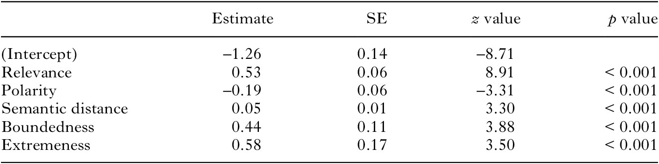

Fig. 7. Model predictions for Experiment 2; ribbons and error bars represent the 95% confidence intervals.
We replicate the findings for relevance, polarity, semantic distance, and boundedness. However, we do not replicate the finding for extremeness. While Gotzner et al. (Reference Gotzner, Solt and Benz2018) found that scales with non-extreme stronger adjectives gave rise to more SIs, we find the opposite: scales with extreme stronger adjectives yielded higher SI rates. This conflicting pattern of results is explored below. The variance explained by our model is 8%, matching the 8% explained by the fixed effects in Experiment 1. Relevance alone constitutes 4% of this variance; the other four factors together have an R 2 of 4%. In sum, we replicate most of the expected effects, but there is still a great deal of variance left to be explained in future work.
4. General discussion
4.1. summary of results
Determining relevance is an essential capability of human cognition; considering all stimuli relevant all the time would be impossible (Vervaeke, Lillicrap, & Richards, Reference Vervaeke, Lillicrap and Richards2012). Context clearly affects what is relevant and what is not, as we saw in the opening example with the sand on the beach, but in out-of-the-blue contexts, we argue that people default to a more general notion of relevance that they have learned by generalising over past experiences in context. In this paper, we have aimed to approximate the general relevance of a scalar inferences based on the frequency with which a weak adjective co-occurs with a stronger adjective in scalar constructions.
In Experiments 1 and 2, our measure of relevance is significantly positively associated with each adjective’s SI rate. This supports the idea that usage provides insight into the cognitive representations of adjectival scales. Further, previously observed effects of polarity, semantic distance, and boundedness were replicated in both experiments. First, more negative scales have a higher SI rate than more positive ones. Second, SI rates increase as semantic distance increases. Third, bounded scales have significantly higher SI rates than unbounded ones.Footnote 1
The effect that we did not replicate was extremeness. In Gotzner et al. (Reference Gotzner, Solt and Benz2018), and in our Experiment 1 using their data, scales with non-extreme stronger adjectives yielded higher SI rates. The opposite was found in Experiment 2: there, scales with extreme stronger adjectives gave rise to more SIs. Gotzner et al. relate their finding to an analysis of the semantics of extreme adjectives by Beltrama and Xiang (Reference Beltrama and Xiang2013, p. 96). These authors state that extreme adjectives cannot be located on lexical scales, since extreme adjectives contain no degree arguments in their meaning. Therefore, they are not available as potential alternatives for the purposes of computing an SI.
However, this analysis is only possible because Beltrama and Xiang (Reference Beltrama and Xiang2013, p. 84) define extremeness such that only non-gradable adjectives can be classified as extreme; gradable adjectives are excluded. If exclusively non-gradable adjectives can be extreme, then it follows that extreme adjectives do not involve degree. But if both gradable and non-gradable adjectives are allowed to be extreme (as in, e.g., Morzycki, Reference Morzycki2012, and indeed Gotzner et al., Reference Gotzner, Solt and Benz2018, and here), this argumentation may not apply. We do not attempt here to resolve the issue of how to define adjectival extremeness. We will say, however, that the pattern of results from Experiment 2 supports the long-standing idea that orientation toward the endpoint matters greatly for SI computation. We also emphasise that the significant positive effect of extremeness of the stronger adjective on the SI rate of the weaker adjective is in line with Gotzner et al.’s original hypothesis.
To resolve this contradiction and estimate the true effect of adjectival extremeness on SI rate, it would be helpful to conduct more experiments that test the effect of extremeness and then perform a meta-analysis of the estimates in these studies. Such an analysis can distill out the by-study variation and approximate the latent effect of extremeness on SI rate (for an example from psycholinguistics, see Jäger, Engelmann, & Vasishth, Reference Jäger, Engelmann and Vasishth2017). It would also shed light on why the results of Experiments 1 and 2 conflict by indicating whether the difference is more likely to be, e.g., a confound in one experiment but not the other or the result of a statistical fluke.
4.2. new angles through new operationalisations
One important methodological contribution of the present paper is the introduction of novel, usage-based operationalisations of four predictors that have been said to underlie scalar inferencing. The results of our experiments show that these operationalisations are good approximations of the judgment-based measures employed in Gotzner et al.’s (Reference Gotzner, Solt and Benz2018) original study, insofar as they reproduce (most of) the observed effects.
We believe that the congruence of judgment-based measures with usage-based ones further underlines the substantial role that usage plays for our linguistic knowledge: it makes sense that frequent co-occurrence of an adjective with, say, a totality modifier correlates with judgments of how natural that adjective is when used together with that modifier, and thus that both measures of boundedness would predict SI rate in the same way. And by synthesising different aspects of the construct of polarity, for instance, we may better approximate its true underlying nature. Thus, in addition to their advantages of reducing subjectivity and combining multiple sources of evidence, the measures we use offer new angles from which to approach our linguistic knowledge.
4.3. questions under discussion and relevance
Throughout this paper, we have relied on a mostly informal understanding of relevance, which was sufficient for our purposes. However, this understanding can be made more precise based on the notion of the question under discussion (QUD). Conversation normally transpires against the backdrop of one or more QUDs. QUDs are usually defined as partitionings on the set of possible worlds (e.g., Roberts, Reference Roberts1996). For example, when it is contextually clear that somebody is interested in learning whether or not they can walk on the beach without shoes, the QUD carves up the set of possible worlds into those where the sand is hot and those where it is not. Based on this notion of QUD, a proposition is said to be relevant insofar as it rules out at least one of the partitions. Thus, in the case at hand, the SI from The sand is warm to The sand is not hot is relevant because it rules out the possible worlds where the sand is hot.
There is an intimate connection between the derivation of SIs and the QUD-relative notion of relevance, such that SIs are more likely to be derived if they help resolve the QUD. It has even been argued that SIs are only derived if they are relevant to the QUD, though experimental evidence suggests that this categorical claim is too strong (e.g., van Kuppevelt, Reference van Kuppevelt1996; Zondervan, Reference Zondervan2010).
Participants in our experiments were only provided with an underspecified context, and hence had to piece together the most likely QUD based on the information given in the utterance itself. Consequently, differences in relevance may correspond to differences in participants’ reconstructions of the QUD. To illustrate, compare painful, which robustly licensed the SI not deadly (80% of the time in Experiment 2) and emotional, which was rarely judged to imply not sentimental (5%). It may be the case that a sentence like The sting is painful tends to be associated with a QUD that makes the SI relevant (e.g., Is the sting just painful, or is it deadly?), whereas the sentence The film was emotional tends to be associated with a QUD that does not (e.g., How was the film?).
This explanation ties in with earlier work of Cummins and Rohde (Reference Cummins and Rohde2015), who manipulated the QUD, and consequently the relevance of the SI, by means of phonological stress, and it also makes several empirically testable predictions. First, it should be possible to measure the frequency of different reconstructions of the QUD by asking participants to indicate the most likely QUD in the given scenario. Second, it is predicted that the degree of scalar diversity is substantially reduced when participants are provided with an explicit question instead of having to reconstruct the QUD.
Inroads have recently been made into studying such questions, e.g., by Ronai and Xiang (Reference Ronai and Xiang2021). Their Experiment 3 relates to our first question, since it proposes a way to measure which QUDs are more likely in a given context by forcing participants to choose between a QUD containing the weaker scalar term and one containing the stronger term (e.g., when describing a student, the experiment tests whether participants would be more likely to ask “Is the student intelligent?” or “Is the student brilliant?”; p. 657). Ronai and Xiang find that the proportion of times that participants chose the question containing the strong term predicts scalar diversity only for unbounded adjectives, and they reason that the scalar endpoint is salient enough already that it does not benefit from the boost provided by the QUD (p. 659). Additionally, Ronai and Xiang’s Experiment 2 relates to our second prediction: they find that an explicit QUD containing the stronger term (e.g., “Is the student brilliant?”) heightens SI rates compared to one with the weaker term (e.g., “Is the student intelligent?”). However, providing an explicit QUD does not fully eliminate scalar diversity (p. 656).
4.4. the effect of usage on the common ground
The preceding discussion in this paper has taken an addressee-based perspective, since SI rates concern the probability that an addressee will draw an SI when they encounter a weak scalar adjective. However, we can also take an addresser-based angle. An addresser always has the choice whether to express their ideas explicitly or via implicature, and what affects their decision is what they know that their interlocutor knows, i.e., what they know to be in the common ground (Diessel, Reference Diessel and Aronoff2017, Woensdregt & Smith, Reference Woensdregt, Smith and Aronoff2017). There is no point to using implicature if the addressee cannot conduct the pragmatic reasoning required to understand what the addresser means to convey.
So, in order to use an SI, e.g., to communicate warm but not hot by only producing warm, the addresser must know that the addressee knows that the SI from warm to warm but not hot is relevant (and that the addressee knows that the addresser knows this too). One way that the addresser can know all of this is usage. If the addresser has frequently experienced warm being used with stronger scalemates, then the fact that the meaning of warm excludes the meaning of the stronger scalemate is relevant for them, but they can also assume that their addressee has encountered it too and built up the same association. In this way, the common ground incorporates linguistic knowledge that has been established by usage over time. This account also lines up with the finding that children tend to draw fewer SIs than adults; they have had less time to establish common ground through usage (van Tiel et al., Reference van Tiel, van Miltenburg, Zevakhina and Geurts2016, p. 169).
Exposure to language use informing the common ground is not a new idea. Studies on lexical entrainment by, e.g., Metzing and Brennan (Reference Metzing and Brennan2003), Grodner and Sedivy (Reference Grodner, Sedivy, Gibson and Pearlmutter2011), and sources therein show that people choose their utterances based on previous usage of particular terms. To our knowledge, though, our study is the first to show how the effect of usage on the common ground can influence the process of scalar inferencing.
5. Conclusions and outlook
We would expect our core proposal – that a usage-based measure of relevance affects SI rates – to generalise beyond adjectives to other classes of scalar expressions that can appear in similar constructions, particularly open classes like nouns and verbs. Table 5 shows some examples of verbal and nominal scales that appear in the scalar construction α but not β in ENCOW16A.
TABLE 5. Example nominal and verbal scales from ENCOW16A

Certainly, some of the factors we test here, like polarity and extremeness, are specific to adjectives, so our analysis will not generalise wholesale. But scalar terms from other parts of speech also have their own particular properties (e.g., quantifiers have monotonicity, verbs telicity) that may play their own roles in their respective classes. Overall, we would expect that the general notion of relevance we discuss here is important for all classes of scalar words.
Since van Tiel et al. (Reference van Tiel, van Miltenburg, Zevakhina and Geurts2016), research on factors that predict scalar diversity has been lively and ongoing. It will soon be time to step back and take stock of everything we have learned. Work in the near future should combine all identified predictors – all the factors from previous work, as well as relevance – to determine how much variance in SI rates has been explained, and how much has yet to be.
In sum, with a usage-based operationalisation of relevance, we have shown that relevance is a significant predictor of diversity in SI rates in adjectives above and beyond the already observed measures of semantic distance, polarity, boundedness, and extremeness. We believe that our findings exemplify the promising and hitherto little-explored viability of usage-based approaches to pragmatic inferencing.


 Open access