


1. Introduction
The study of centrality in networks goes back to the late forties. Since then, several measures of centrality with different properties have been proposed—see Boldi & Vigna (Reference Boldi and Vigna2014) for a survey. To sort out which measures are more apt for a specific application, one can try to classify them through some axioms that they might satisfy or not.
In Boldi & Vigna (Reference Boldi and Vigna2014), Boldi et al. (Reference Boldi, Luongo and Vigna2017), two of the authors studied in particular score monotonicity and rank monotonicity on directed graphs. The first property says that when an arc
 $x\to y$
is added to the graph, the score of
$x\to y$
is added to the graph, the score of
 $y$
strictly increases (Sabidussi, Reference Sabidussi1966). Rank monotonicity (Chien et al., Reference Chien, Dwork, Kumar, Simon and Sivakumar2004) states that after adding an arc
$y$
strictly increases (Sabidussi, Reference Sabidussi1966). Rank monotonicity (Chien et al., Reference Chien, Dwork, Kumar, Simon and Sivakumar2004) states that after adding an arc
 $x\to y$
, all nodes with a score smaller than (or equal to)
$x\to y$
, all nodes with a score smaller than (or equal to)
 $y$
still have a score smaller than (or equal to)
$y$
still have a score smaller than (or equal to)
 $y$
. Score and rank monotonicity complement themselves: score monotonicity tells us that “something good happens”; rank monotonicity tells us that “nothing bad happens.”
$y$
. Score and rank monotonicity complement themselves: score monotonicity tells us that “something good happens”; rank monotonicity tells us that “nothing bad happens.”
In some way, both axioms aim at answering the following question: is it always worth it for a node in a directed social network (say, Twitter) to have a new incoming arc (in Twitter parlance, a new follower)? The two monotonicity axioms introduced above give a different interpretation of what “worth” means. “Score monotonicity” interprets it simply as an increase of score: if you get a new follower, does your score always increase? “Rank monotonicity” interprets it with respect to the score of other nodes: if you get a new follower, do you still dominate (have a larger score than) the same nodes you used to dominate before, and possibly more? As we said, for most notions of importance (i.e., centrality measures) the answer to both questions is “yes,” under very mild assumptions (Boldi et al., Reference Boldi, Luongo and Vigna2017).
Once we move to undirected graphs, however, previous definitions and results are no longer applicable. Thus, in this paper, we aim at answering a subtly different question: is it always worth it for an actor in an undirected social network (say, Facebook) to have a new friend? Again, “worth” can be taken to refer to its score or to its rank. In this paper, we propose more precise definitions that are natural extensions of score and rank monotonicity to the undirected case and prove results about classical centrality measures: closeness (Bavelas, Reference Bavelas1948), harmonic centrality (Beauchamp, Reference Beauchamp1965), betweenness (Anthonisse, Reference Anthonisse1971; Freeman, Reference Freeman1977), and four variants of spectral ranking (Vigna, Reference Vigna2016)—eigenvector centrality (Landau, Reference Landau1895; Berge, Reference Berge1958), Katz’s index (Katz, Reference Katz1953), Seeley’s index (Seeley, Reference Seeley1949), and PageRank (Page et al., Reference Page, Brin, Motwani and Winograd1998).
As we will see, while in some cases we can witness some score increase, except for Seeley’s index none of the centrality measures we consider is rank monotone. This is somehow surprising and will yield some reflection.
Note that adding a single edge to an undirected graph is equivalent to adding two opposite arcs in a directed graph, which may suggest why the situation is so different, at least from the mathematical viewpoint. Understanding under which conditions a centrality measure does not satisfy an axiom will be a theme that we will try to pursue in the course of the discussion.
We provide classes of counterexamples of arbitrary size; moreover, we always provide both a counterexample in which the loss of rank happens in the less important endpoint of the new edge and a counterexample in which the loss of rank happens in the more important endpoint of the new edge. In this way, we will show that it is impossible for the two actors in the social network creating the new edge to predict whether the edge will be beneficial even knowing their relative importance. The results obtained in this paper are summarized in Table 1.
Table 1. Summary of the results of this paper for the case of connected undirected graphs. For comparison, recall that (Boldi et al., Reference Boldi, Luongo and Vigna2017) all the centrality measures listed are both score and rank monotone on strongly connected directed graphs, with the only exception of betweenness that is neither. We include degree (which is trivially score monotone and strictly rank monotone on all graphs) for completeness

To prove general results in the case of spectral rankings, we exploit the connection between spectral rankings and graph fibrations (Boldi & Vigna, Reference Boldi and Vigna2002; Boldi et al., Reference Boldi, Lonati, Santini and Vigna2006), which makes us able to reduce computations on graphs with a variable number of nodes to similar computations on graphs with a fixed number of nodes. This approach to proofs, which we believe is of independent interest, makes it possible to use analytic techniques to control the values assumed by eigenvector centrality, Katz’s index, and PageRank.
We conclude the paper with some anecdotal evidence from a medium-sized real-world network, showing that violations of monotonicity do happen also in practice.
Most of the computations in this paper (in particular, the manipulation of complex rational functions) have been performed using Sage (The Sage Developers, 2018). All our Sage worksheets are available as public-domain software on the Zenodo platform.Footnote 1
2. Graph-theoretical preliminaries
While we will focus on simple undirected graphs, we are going to make use of some proof techniques that require handling more general types of graphs.
A (directed multi)graph
 $G$
is defined by a set
$G$
is defined by a set
 $N_G$
of nodes, a set
$N_G$
of nodes, a set
 $A_G$
of arcs, and by two functions
$A_G$
of arcs, and by two functions
 $s_G,t_G\,:\,A_G\to N_G$
that specify the source and the target of each arc; a loop is an arc with the same source and target; the main difference between this definition and the standard definition of a directed graph is that we allow for the presence of multiple arcs between a pair of nodes. When we do not need to distinguish between multiple arcs, we write
$s_G,t_G\,:\,A_G\to N_G$
that specify the source and the target of each arc; a loop is an arc with the same source and target; the main difference between this definition and the standard definition of a directed graph is that we allow for the presence of multiple arcs between a pair of nodes. When we do not need to distinguish between multiple arcs, we write
 $x\to y$
to denote an arc with source
$x\to y$
to denote an arc with source
 $x$
and target
$x$
and target
 $y$
.
$y$
.
Since we do not need to discriminate between graphs that only differ because of node names, we will often assume that
 $N_G=\{\,0,1,\dots,n_G-1\,\}$
where
$N_G=\{\,0,1,\dots,n_G-1\,\}$
where
 $n_G$
is the number of nodes of
$n_G$
is the number of nodes of
 $G$
. Every graph
$G$
. Every graph
 $G$
has an associated
$G$
has an associated
 $n_G \times n_G$
adjacency matrix, also denoted by
$n_G \times n_G$
adjacency matrix, also denoted by
 $G$
, where
$G$
, where
 $G_{xy}$
is the number of arcs from
$G_{xy}$
is the number of arcs from
 $x$
to
$x$
to
 $y$
.
$y$
.
A (simple) undirected graph is a looplessFootnote
2
graph
 $G$
such that for all
$G$
such that for all
 $x,y \in N_G$
we have
$x,y \in N_G$
we have
 $G_{xy}=G_{yx}\leq 1$
. In other words, there is at most one arc between any two nodes, and if there is an arc from
$G_{xy}=G_{yx}\leq 1$
. In other words, there is at most one arc between any two nodes, and if there is an arc from
 $x$
to
$x$
to
 $y$
, there is also an arc in the opposite direction. In an undirected graph, an edge between
$y$
, there is also an arc in the opposite direction. In an undirected graph, an edge between
 $x$
and
$x$
and
 $y$
is a pair of arcs
$y$
is a pair of arcs
 $x\to y$
and
$x\to y$
and
 $y\to x$
, and it is denoted by
$y\to x$
, and it is denoted by
 $x\mbox{---}y$
. This definition is equivalent to the more common notion that an edge is an unordered set of nodes, but it makes it possible to mix undirected and directed graphs: indeed, even in drawings we will freely mix arcs and edges. For undirected graphs, we prefer to use the word “vertex” instead of “node.”
$x\mbox{---}y$
. This definition is equivalent to the more common notion that an edge is an unordered set of nodes, but it makes it possible to mix undirected and directed graphs: indeed, even in drawings we will freely mix arcs and edges. For undirected graphs, we prefer to use the word “vertex” instead of “node.”
3. Score and rank monotonicity axioms on undirected graphs
One of the most important notions that researchers have been trying to capture in various types of graphs is “node centrality”: ideally, every node (often representing an individual) has some degree of influence or importance within the social domain under consideration, and one expects such importance to be reflected in the structure of the social network; centrality is a quantitative measure that aims at revealing the importance of a node.
Formally, a centrality (measure or index) is any function
 $c$
that, given a graph
$c$
that, given a graph
 $G$
, assigns a real number
$G$
, assigns a real number
 $c_G(x)$
to every node
$c_G(x)$
to every node
 $x$
of
$x$
of
 $G$
, with larger values implying more importance. Countless notions of centrality have been proposed over time, for different purposes and with different aims; some of them were originally defined only for a specific category of graphs. Later some of these notions of centrality have been extended to more general classes; all centrality measures discussed in this paper can be defined properly on all undirected graphs (even disconnected ones). We assume from the beginning that the centrality measures under examination are invariant by isomorphism; that is, that they depend just on the structure of the graph and not on a particular name chosen for each node. In particular, all nodes exchanged by an automorphism necessarily share the same centrality score, and we will use this fact to simplify our computations.
$G$
, with larger values implying more importance. Countless notions of centrality have been proposed over time, for different purposes and with different aims; some of them were originally defined only for a specific category of graphs. Later some of these notions of centrality have been extended to more general classes; all centrality measures discussed in this paper can be defined properly on all undirected graphs (even disconnected ones). We assume from the beginning that the centrality measures under examination are invariant by isomorphism; that is, that they depend just on the structure of the graph and not on a particular name chosen for each node. In particular, all nodes exchanged by an automorphism necessarily share the same centrality score, and we will use this fact to simplify our computations.
Axioms are useful to isolate properties of different centrality measures and make it possible to compare them. One of the oldest papers to propose this approach is Sabidussi (Reference Sabidussi1966), which introduced score monotonicity, and many other proposals have appeared in the last few decades.
In this paper, we will be dealing with two properties of centrality measures:
Definition 1. (Score monotonicity) Given an undirected graph
 $G$
, a centrality
$G$
, a centrality
 $c$
is said to be score monotone on
$c$
is said to be score monotone on
 $G$
iff for every pair of non-adjacent vertices
$G$
iff for every pair of non-adjacent vertices
 $x$
and
$x$
and
 $y$
we have that
$y$
we have that
 \begin{equation*} c_G(x) \lt c_{G^{\prime}}(x) \quad \text {and}\quad c_G(y) \lt c_{G^{\prime}}(y), \end{equation*}
where
 $G^{\prime}$
is the graph obtained adding the new edge
$G^{\prime}$
is the graph obtained adding the new edge
 $x-y$
to
$x-y$
to
 $G$
. We say that
$G$
. We say that
 $c$
is score monotone on undirected graphs iff it is score monotone on all undirected graphs.
$c$
is score monotone on undirected graphs iff it is score monotone on all undirected graphs.
Definition 2. (Rank monotonicity) Given an undirected graph
 $G$
, a centrality
$G$
, a centrality
 $c$
is said to be rank monotone
Footnote
3
on
$c$
is said to be rank monotone
Footnote
3
on
 $G$
iff for every pair of non-adjacent vertices
$G$
iff for every pair of non-adjacent vertices
 $x$
and
$x$
and
 $y$
we have that for all vertices
$y$
we have that for all vertices
 $z\neq x,y$
 \begin{equation*} c_G(z) \lt c_{G}(x) \Rightarrow c_{G^{\prime}}(z) \lt c_{G^{\prime}}(x) \quad {and}\quad c_G(z) \lt c_{G}(y) \Rightarrow c_{G^{\prime}}(z) \lt c_{G^{\prime}}(y), \end{equation*}
and moreover
 \begin{equation*} c_G(z) \leq c_{G}(x) \Rightarrow c_{G^{\prime}}(z)\leq c_{G^{\prime}}(x) \quad {and}\quad c_G(z)\leq c_{G}(y) \Rightarrow c_{G^{\prime}}(z) \leq c_{G^{\prime}}(y), \end{equation*}
where
 $G^{\prime}$
is the graph obtained adding the new edge
$G^{\prime}$
is the graph obtained adding the new edge
 $x-y$
to
$x-y$
to
 $G$
. It is said to be strictly rank monotone on
$G$
. It is said to be strictly rank monotone on
 $G$
if instead
$G$
if instead
 \begin{equation*} c_G(z) \leq c_{G}(x) \Rightarrow c_{G^{\prime}}(z) \lt c_{G^{\prime}}(x) \quad {and}\quad c_G(z) \leq c_{G}(y) \Rightarrow c_{G^{\prime}}(z) \lt c_{G^{\prime}}(y) \end{equation*}
We say that
 $c$
is (strictly) rank monotone on undirected graphs iff it is (strictly) rank monotone on all undirected graphs.
$c$
is (strictly) rank monotone on undirected graphs iff it is (strictly) rank monotone on all undirected graphs.
Score monotonicity tells us that in absolute terms, the new edge is beneficial to
 $x$
and
$x$
and
 $y$
. Rank monotonicity tells us that in relative terms, the new edge is not hurting them, in the sense that nodes that were (strictly) dominated by
$y$
. Rank monotonicity tells us that in relative terms, the new edge is not hurting them, in the sense that nodes that were (strictly) dominated by
 $x$
or
$x$
or
 $y$
are still (strictly) dominated. Finally, strict rank monotonicity is a stronger property that implies, besides preservation of dominance, an improvement, as additionally all nodes in a score tie with
$y$
are still (strictly) dominated. Finally, strict rank monotonicity is a stronger property that implies, besides preservation of dominance, an improvement, as additionally all nodes in a score tie with
 $x$
or
$x$
or
 $y$
will have a strictly smaller score after adding the new edge. As a sanity check, we note that degree, the simplest centrality measure, is both score monotone and strictly rank monotone.
$y$
will have a strictly smaller score after adding the new edge. As a sanity check, we note that degree, the simplest centrality measure, is both score monotone and strictly rank monotone.
These three properties can be studied on the class of all undirected graphs or only on the class of connected graphs, giving rise to six possible “degrees of monotonicity” that every given centrality may satisfy or not. This paper studies these different degrees of monotonicity for some of the most popular centrality measures, also comparing the result obtained with the corresponding properties in the directed case.
With respect to the directed case, there is an important difference: violation of the axioms may happen on one of the nodes involved, or on both. While we never witnessed the latter situation, there is in the first case a distinction that we feel important enough to deserve a name:
Definition 3. A violation of score monotonicity is a top violation if the endpoint of the new edge whose scores decreases is more important than the other. It is a bottom violation otherwise. The same distinction applies to violations of rank monotonicity.
Top violations are somewhat sociologically natural: if a network superstar becomes friend with a nobody, it is not surprising that the nobody increases their popularity, whereas the superstar loses a bit of charm. Bottom violations, however, are much less natural: in the same context, the nobody sees their importance decrease, nurturing in a bizarre inversion of flow the superstar popularity.
As we already anticipated, and differently from the directed case, all centrality measures we consider, except for Seeley’s index (which however is trivial in this context—see Section 9) will turn out to be not rank monotone. Moreover, most centralities are not score monotone. As a consequence, this paper is a sequence of counterexamples (to score monotonicity and to rank monotonicity, hence a fortiori to its strict version): all counterexamples exhibit an undirected graph
 $G$
and two non-adjacent vertices
$G$
and two non-adjacent vertices
 $x$
and
$x$
and
 $y$
such that when you add the edge
$y$
such that when you add the edge
 $x-y$
to
$x-y$
to
 $G$
,
$G$
,
 $x$
decreases its score, or its rank with respect to some other vertex
$x$
decreases its score, or its rank with respect to some other vertex
 $z$
. We may call
$z$
. We may call
 $x$
the “losing endpoint” (i.e., the one that is hurt by the addition of the edge).
$x$
the “losing endpoint” (i.e., the one that is hurt by the addition of the edge).
Not all counterexamples are equally good, though. We will make an effort to have the theoretically strongest counterexamples we can find, and we will also look for properties that have a practical interpretation. More in detail:
-
all our counterexamples are connected;
-
all our counterexamples are parametric graphs that can be instantiated in graphs of arbitrarily large size;
-
we always give both top and bottom violation counterexamples; thus, even knowing whether you are more or less important than your new neighbor will not help in knowing if you will gain or lose from the new edge;
-
in all our counterexamples the losing endpoint of the new edge is also demoted; that is, the number of nodes with a larger score than the losing endpoint increases after adding the new edge.
The last point is particularly important because demotion is not implied by the lack of rank monotonicity: it may be the case that
 $x$
used to be more important than
$x$
used to be more important than
 $z$
and it becomes less important than
$z$
and it becomes less important than
 $z$
after the addition of the edge
$z$
after the addition of the edge
 $x-y$
, but still the number of nodes that are more important than
$x-y$
, but still the number of nodes that are more important than
 $x$
becomes smaller with the addition of
$x$
becomes smaller with the addition of
 $x-y$
. The lack of demotion might suggest a weaker notion of rank monotonicity, in which the number of nodes whose score dominates
$x-y$
. The lack of demotion might suggest a weaker notion of rank monotonicity, in which the number of nodes whose score dominates
 $x$
(or
$x$
(or
 $y$
) decreases (such a notion is strictly weaker as it is implied by rank monotonicity). However, this weaker notion is not very appealing from a practical viewpoint, because it is not locally testable—it has no immediate consequence for the relative importance of an endpoint of the edge and another vertex. Proving demotion implies that the counterexamples in this paper are strong enough to violate also the weaker notion of monotonicity described above.
$y$
) decreases (such a notion is strictly weaker as it is implied by rank monotonicity). However, this weaker notion is not very appealing from a practical viewpoint, because it is not locally testable—it has no immediate consequence for the relative importance of an endpoint of the edge and another vertex. Proving demotion implies that the counterexamples in this paper are strong enough to violate also the weaker notion of monotonicity described above.
4. Geometric centralities
Since adding a new edge can only shorten existing shortest paths or create new ones, it is immediate to show that harmonic centrality is score monotone; for the same reason, closeness centrality is score monotone on connected graphs, whereas counterexamples similar to those of the directed case of Boldi & Vigna (Reference Boldi and Vigna2014) prove that closeness is not score monotone in the general case.
Less intuitively, neither closeness nor harmonic centrality are rank monotone in the undirected case. The family of counterexamples we found shows that adding an edge can shorten distances in ways that are much more useful for some vertices not incident on the new edge than on its endpoints.
Our counterexample for rank monotonicity of closeness and harmonic centrality is shown in Figure 1. The idea behind the graph is that the edge
 $0-1$
reduces the distance between vertex
$0-1$
reduces the distance between vertex
 $0$
and the vertices labeled with
$0$
and the vertices labeled with
 $4$
, but does not reduce the distance between vertex
$4$
, but does not reduce the distance between vertex
 $0$
and vertex
$0$
and vertex
 $3$
(and more importantly between vertex
$3$
(and more importantly between vertex
 $0$
and the star around vertex
$0$
and the star around vertex
 $3$
). Thus, the vertices labeled with
$3$
). Thus, the vertices labeled with
 $4$
will gain more centrality from the new edge than vertex
$4$
will gain more centrality from the new edge than vertex
 $0$
, and for appropriate values of
$0$
, and for appropriate values of
 $j$
and
$j$
and
 $k$
, we will be able to prove a violation of rank monotonicity (all vertices labeled with
$k$
, we will be able to prove a violation of rank monotonicity (all vertices labeled with
 $4$
share the same centrality). The stars of size
$4$
share the same centrality). The stars of size
 $r$
around vertex
$r$
around vertex
 $1$
and vertex
$1$
and vertex
 $2$
will instead be useful by giving us some more space to play with the relative importance of the endpoints of the new edge, tuning the graph in Figure 1 to be an example of top or bottom violation.
$2$
will instead be useful by giving us some more space to play with the relative importance of the endpoints of the new edge, tuning the graph in Figure 1 to be an example of top or bottom violation.

Figure 1. A counterexample to rank monotonicity for closeness and harmonic centrality. There is a star with
 $j$
leaves around vertex
$j$
leaves around vertex
 $0$
, a star with
$0$
, a star with
 $k$
leaves around vertex
$k$
leaves around vertex
 $3$
, a star with
$3$
, a star with
 $r$
leaves around vertex
$r$
leaves around vertex
 $1$
, and a star with
$1$
, and a star with
 $r$
leaves around vertex
$r$
leaves around vertex
 $2$
. Before adding the edge
$2$
. Before adding the edge
 $0-1$
, the score of vertex
$0-1$
, the score of vertex
 $0$
is larger than the score of the vertices labeled with
$0$
is larger than the score of the vertices labeled with
 $4$
; after, it is smaller.
$4$
; after, it is smaller.
4.1 Closeness
We recall that closeness of a vertex
 $x$
is defined as the reciprocal of its peripherality
$x$
is defined as the reciprocal of its peripherality
 \begin{equation*} p(x)=\sum _{y\in N_G}d(x,y), \end{equation*}
where
 $d(x,y)$
is the distance (i.e., the length of a shortest path) between
$d(x,y)$
is the distance (i.e., the length of a shortest path) between
 $x$
and
$x$
and
 $y$
.
$y$
.
We denote for simplicity with
 $\textrm{pre}({-})$
and
$\textrm{pre}({-})$
and
 $\textrm{post}({-})$
the peripherality of the graph in Figure 1 before and after adding the edge
$\textrm{post}({-})$
the peripherality of the graph in Figure 1 before and after adding the edge
 $0-1$
. Then,
$0-1$
. Then,
 \begin{align*} \textrm{pre}(0)&=15 + j + 4 k + 11r & \textrm{post}(0)&=9 + j + 4 k + 5r \\ \textrm{pre}(1)&=15 +6j + 3 k + 3r & \textrm{post}(1)&=9 + 2j + 3 k + 3r \\ \textrm{pre}(4)&=15 + 6j + 3 k + 5r & \textrm{post}(4)&=13 + 4j + 3 k + 5r. \end{align*}
We are interested in finding solutions, if they exists, to the set of inequalities
 \begin{equation*} \textrm {pre}(0) \gt \textrm {pre}(1), \textrm {pre}(0)\lt \textrm {pre}(4), \textrm {post}(0)\gt \textrm {post}(4), \end{equation*}
which specify that vertex
 $0$
violates rank monotonicity with respect to vertices labeled with
$0$
violates rank monotonicity with respect to vertices labeled with
 $4$
and that it is less important than vertex
$4$
and that it is less important than vertex
 $1$
(recall we are manipulating the reciprocal of closeness), and
$1$
(recall we are manipulating the reciprocal of closeness), and
 \begin{equation*} \textrm {pre}(0) \lt \textrm {pre}(1), \textrm {pre}(0)\lt \textrm {pre}(4), \textrm {post}(0)\gt \textrm {post}(4), \end{equation*}
that correspond to the analogous case in which vertex
 $0$
is more important than vertex
$0$
is more important than vertex
 $1$
. There are infinite solutions for both sets of inequalities, and in particular,
$1$
. There are infinite solutions for both sets of inequalities, and in particular,
 $j=5r$
,
$j=5r$
,
 $k=18r$
(
$k=18r$
(
 $r\geq 2$
), and
$r\geq 2$
), and
 $j=4r+4$
,
$j=4r+4$
,
 $k=12r+17$
(
$k=12r+17$
(
 $r\geq 1$
) satisfy the first and second set, respectively.
$r\geq 1$
) satisfy the first and second set, respectively.
Theorem 1.
Closeness is not rank monotone on the graphs of Figure
1
for
 $r\geq 2$
,
$r\geq 2$
,
 $j=5r$
, and
$j=5r$
, and
 $k=18r$
(bottom violation) and for
$k=18r$
(bottom violation) and for
 $r\geq 1$
,
$r\geq 1$
,
 $j=4r+4$
, and
$j=4r+4$
, and
 $k=12r+17$
(top violation).
$k=12r+17$
(top violation).
While the family of graphs we consider contains graphs of unbounded size, each graph has just ten distinct peripherality scores. We can thus compare exactly the peripherality of all vertices with that of vertex
 $0$
before and after adding the new edge. It is easy to see that for the parameter sets of the previous theorem, all vertices, except the
$0$
before and after adding the new edge. It is easy to see that for the parameter sets of the previous theorem, all vertices, except the
 $j$
vertices labeled with
$j$
vertices labeled with
 $4$
and sometimes vertex 1, maintain the same relative position to vertex
$4$
and sometimes vertex 1, maintain the same relative position to vertex
 $0$
after adding the edge
$0$
after adding the edge
 $0-1$
. Thus, in both cases vertex
$0-1$
. Thus, in both cases vertex
 $0$
is demoted by at least
$0$
is demoted by at least
 $j-1$
positions.
$j-1$
positions.
4.2 Harmonic centrality
The counterexample in Figure 1 works also for harmonic centrality, which is not surprising as the only difference between closeness and harmonic centrality is the usage of a harmonic mean instead of an arithmetic mean.
Denoting this time with
 $\textrm{pre}({-})$
and
$\textrm{pre}({-})$
and
 $\textrm{post}({-})$
the harmonic centrality of the graph in Figure 1 before and after adding the edge
$\textrm{post}({-})$
the harmonic centrality of the graph in Figure 1 before and after adding the edge
 $0-1$
, we have
$0-1$
, we have
 \begin{align*} \textrm{pre}(0)&=\frac{137}{60} + j + \frac 14k + \frac{11}{30}r & \textrm{post}(0)&=\frac{10}{3} + j + \frac 14k + \frac 56r \\[4pt] \textrm{pre}(1)&=\frac{137}{60} + \frac 16j + \frac 13k +\frac 32r & \textrm{post}(1)&=\frac{10}{3} + \frac 12j + \frac 13k + \frac 32r\\[4pt] \textrm{pre}(4)&= \frac{137}{60}+ \frac 16j + \frac 13k + \frac 56r & \textrm{post}(4)&=\frac{29}{12} + \frac 14j + \frac 13k + \frac 56r . \end{align*}
This time we are interested in finding solutions, if they exists, to the set of inequalities
 \begin{equation*} \textrm {pre}(0) \lt \textrm {pre}(1), \textrm {pre}(0)\gt \textrm {pre}(4), \textrm {post}(0)\lt \textrm {post}(4) \end{equation*}
and
 \begin{equation*} \textrm {pre}(0) \gt \textrm {pre}(1), \textrm {pre}(0)\gt \textrm {pre}(4), \textrm {post}(0)\lt \textrm {post}(4). \end{equation*}
There are again infinite solutions for both sets of inequalities, and in particular,
 $j=26r$
,
$j=26r$
,
 $k=247r$
(
$k=247r$
(
 $r\geq 1$
), and
$r\geq 1$
), and
 $j=26r$
,
$j=26r$
,
 $k=246r$
(
$k=246r$
(
 $r\geq 1$
) satisfy the first and second set, respectively.
$r\geq 1$
) satisfy the first and second set, respectively.
Theorem 2.
Harmonic centrality is not rank monotone on the graphs of Figure
1
for
 $r\geq 1$
,
$r\geq 1$
,
 $j=26r$
, and
$j=26r$
, and
 $k=247r$
(bottom violation) and for
$k=247r$
(bottom violation) and for
 $r\geq 1$
,
$r\geq 1$
,
 $j=26r$
, and
$j=26r$
, and
 $k=246r$
(top violation).
$k=246r$
(top violation).
Also in this case, for the same parameter sets, all vertices, except the
 $j$
vertices labeled with
$j$
vertices labeled with
 $4$
and sometimes vertex
$4$
and sometimes vertex
 $1$
, maintain the same relative position to vertex
$1$
, maintain the same relative position to vertex
 $0$
after adding the edge
$0$
after adding the edge
 $0-1$
. Thus, vertex
$0-1$
. Thus, vertex
 $0$
is demoted by at least
$0$
is demoted by at least
 $j-1$
positions.
$j-1$
positions.
5. Betweenness
Betweenness is neither score nor rank monotone on directed graphs (Boldi et al., Reference Boldi, Luongo and Vigna2017); the same is true in the undirected case, as shown in the graph of Figure 2. Intuitively, the new edge puts
 $2$
on many shortest paths (e.g., those between any vertex labeled with
$2$
on many shortest paths (e.g., those between any vertex labeled with
 $3$
and any vertex labeled with
$3$
and any vertex labeled with
 $4$
) that before needed to pass on the upper route of the rectangle. Vertex
$4$
) that before needed to pass on the upper route of the rectangle. Vertex
 $0$
, instead, does not gain as much by the addition of the edge.
$0$
, instead, does not gain as much by the addition of the edge.
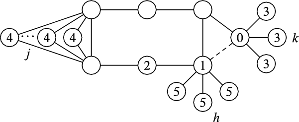
Figure 2. A counterexample to score and rank monotonicity for betweenness. There is a star with
 $k$
leaves around vertex
$k$
leaves around vertex
 $0$
, a star with
$0$
, a star with
 $h$
leaves around vertex
$h$
leaves around vertex
 $1$
, and
$1$
, and
 $j$
vertices labeled with
$j$
vertices labeled with
 $4$
with the same neighborhood. Before adding the edge
$4$
with the same neighborhood. Before adding the edge
 $0-1$
, the score of vertex
$0-1$
, the score of vertex
 $0$
is larger than the score of vertex
$0$
is larger than the score of vertex
 $2$
; after the addition, it becomes smaller. Moreover, the score of vertex 0 does not change when the edge is added.
$2$
; after the addition, it becomes smaller. Moreover, the score of vertex 0 does not change when the edge is added.
Denoting with
 $\textrm{pre}({-})$
and
$\textrm{pre}({-})$
and
 $\textrm{post}({-})$
the value of betweenness before and after adding the edge
$\textrm{post}({-})$
the value of betweenness before and after adding the edge
 $0-1$
, we have
$0-1$
, we have
 \begin{align*} \textrm{pre}(0)&=\frac{k(2h+2j+k+11)}2 & \textrm{post}(0)&=\frac{k(2h+2j+k+11)}2\\ \textrm{pre}(1)&=\frac{h^2+(2j+2k+11)h+3k+7}2 & \textrm{post}(1)&=\frac{h^2+(2j+2k+11)h+(k+1)(j+4)+4}2\\ \textrm{pre}(2)&=\frac{(2h+2)j+3h+k+5}2 & \textrm{post}(2)&=\frac{(2h+k+2)j+3h+2k+6}2 . \end{align*}
Observe that
 $\textrm{pre}(0)=\textrm{post}(0)$
, showing that score monotonicity is violated. To prove that also rank monotonicity does not hold, we are interested in finding solutions to the set of inequalities
$\textrm{pre}(0)=\textrm{post}(0)$
, showing that score monotonicity is violated. To prove that also rank monotonicity does not hold, we are interested in finding solutions to the set of inequalities
 \begin{equation*} \textrm {pre}(0) \lt \textrm {pre}(1), \textrm {pre}(0)\gt \textrm {pre}(2), \textrm {post}(0)\lt \textrm {post}(2) \end{equation*}
and
 \begin{equation*} \textrm {pre}(0) \gt \textrm {pre}(1), \textrm {pre}(0)\gt \textrm {pre}(2), \textrm {post}(0)\lt \textrm {post}(2). \end{equation*}
There are infinite solutions for both sets of inequalities, and in particular,
 $h=k$
,
$h=k$
,
 $j= \lfloor (k^2-4k-15)/2 \rfloor$
,
$j= \lfloor (k^2-4k-15)/2 \rfloor$
,
 $k\geq 13$
, and
$k\geq 13$
, and
 $k=2+h$
,
$k=2+h$
,
 $j=4h$
,
$j=4h$
,
 $h\geq 12$
satisfy the first and second set, respectively.
$h\geq 12$
satisfy the first and second set, respectively.
Theorem 3.
Betweenness is not rank monotone on the graph of Figure
2, for
 $k=2+h$
,
$k=2+h$
,
 $j=4h$
,
$j=4h$
,
 $h\geq 12$
, (top violation) and for
$h\geq 12$
, (top violation) and for
 $h=k$
,
$h=k$
,
 $j= \lfloor (k^2-4k-15)/2 \rfloor$
,
$j= \lfloor (k^2-4k-15)/2 \rfloor$
,
 $k\geq 13$
(bottom violation).
$k\geq 13$
(bottom violation).
Also in this case, we have just nine different betweenness scores, which makes it possible to show that in both cases vertex
 $0$
is demoted by at least one position.
$0$
is demoted by at least one position.
6. Eigenvector centrality
Eigenvector centrality is probably the oldest attempt at deriving a centrality from matrix information: a first version was proposed by Landau (Reference Landau1895) for matrices representing the results of chess tournaments, and it was defined in full generality by Berge (Reference Berge1958); it was rediscovered many times since then. One considers the adjacency matrix of the graph and computes its left or right dominant eigenvector (in our case, the two eigenvectors coincide): the result is thus defined modulo a scaling factor; furthermore, if the graph is (strongly) connected, the result is unique (again, modulo the scaling factor) by the Perron–Frobenius theorem (Berman & Plemmons, Reference Berman and Plemmons1994).
It is not difficult to find anecdotal examples of violation of rank (and even score, fixing a normalization) monotonicity in simple examples. In Figure 3, we show a very simple graph that does not satisfy score monotonicity under the most obvious forms of normalization. In particular, the score of vertex
 $0$
decreases after adding the edge
$0$
decreases after adding the edge
 $0-1$
both in norm
$0-1$
both in norm
 $\ell _1$
and norm
$\ell _1$
and norm
 $\ell _2$
, and even when projecting the constant vectorFootnote
4
$\ell _2$
, and even when projecting the constant vectorFootnote
4
 $\textbf 1$
onto the dominant eigenspace, which is an alternative way of circumventing the scaling factor (Vigna, Reference Vigna2016). The intuition is that once we close the triangle we create a cycle that absorbs a large amount of rank, effectively decreasing the score of vertex
$\textbf 1$
onto the dominant eigenspace, which is an alternative way of circumventing the scaling factor (Vigna, Reference Vigna2016). The intuition is that once we close the triangle we create a cycle that absorbs a large amount of rank, effectively decreasing the score of vertex
 $0$
.
$0$
.
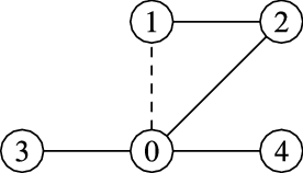
Figure 3. A counterexample to score monotonicity for eigenvector centrality. After adding the edge
 $0-1$
, the score of vertex
$0-1$
, the score of vertex
 $0$
decreases: in norm
$0$
decreases: in norm
 $\ell _1$
, from
$\ell _1$
, from
 $0.30656$
to
$0.30656$
to
 $0.29914$
; in norm
$0.29914$
; in norm
 $\ell _2$
, from
$\ell _2$
, from
 $0.65328$
to
$0.65328$
to
 $0.63586$
, and when projecting the constant vector
$0.63586$
, and when projecting the constant vector
 $\textbf 1$
onto the dominant eigenspace, from
$\textbf 1$
onto the dominant eigenspace, from
 $1.39213$
to
$1.39213$
to
 $1.35159$
.
$1.35159$
.
A similar counterexample, shown in Figure 4, proves that eigenvector centrality does not satisfy rank monotonicity. Before adding the edge
 $0-1$
, the score of vertex
$0-1$
, the score of vertex
 $1$
used to be larger than the score of vertex
$1$
used to be larger than the score of vertex
 $3$
; the converse is true after the addition of the edge. This counterexample, however, is not very satisfactory as vertex
$3$
; the converse is true after the addition of the edge. This counterexample, however, is not very satisfactory as vertex
 $1$
is not demoted—in fact, the opposite happens; on the other hand, the set of vertices that dominate it changes completely with the addition of the new edge, showing that eigenvector centrality can undergo turbulent modifications upon a simple perturbation: this example thus shows that the known sensitivity of eigenvectors to matrix perturbation (Stewart & Sun, Reference Stewart and Sun1990) remains true even in our very restricted setting (dominant eigenvectors of symmetric irreducible 0
$1$
is not demoted—in fact, the opposite happens; on the other hand, the set of vertices that dominate it changes completely with the addition of the new edge, showing that eigenvector centrality can undergo turbulent modifications upon a simple perturbation: this example thus shows that the known sensitivity of eigenvectors to matrix perturbation (Stewart & Sun, Reference Stewart and Sun1990) remains true even in our very restricted setting (dominant eigenvectors of symmetric irreducible 0
 $-$
1 matrices perturbed by setting two symmetric entries to one).
$-$
1 matrices perturbed by setting two symmetric entries to one).
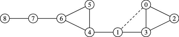
Figure 4. A counterexample to rank monotonicity for eigenvector centrality. Before adding the edge
 $0-1$
, the score of vertex
$0-1$
, the score of vertex
 $1$
is larger than the score of vertex
$1$
is larger than the score of vertex
 $3$
; after, it is smaller.
$3$
; after, it is smaller.
We are now going to prove that eigenvector centrality does not satisfy rank monotonicity on a class of graphs of arbitrarily large size in which we will also experience demotion. Proving analytical results will require combining a few techniques from spectral graph theory and analysis, as we would otherwise not be able to perform exact computations, as in the previous cases.
7. Interlude: Graph fibrations
Proving analytical results about graphs of arbitrary size requires in principle manipulating matrices of arbitrary size, and obtaining closed-form expressions for eigenvalues and eigenvectors of such matrices would be difficult, if not impossible. We thus turn to ideas going back to the results obtained in the ’60s in the context of the theory of graph divisors (Sachs, Reference Sachs1966), restating them in the more recent language of graph fibrations (Boldi & Vigna, Reference Boldi and Vigna2002).
A (graph) morphism
 $\varphi \,:\,G\to H$
is given by a pair of functions
$\varphi \,:\,G\to H$
is given by a pair of functions
 $f_N\,:\,N_G\to N_H$
and
$f_N\,:\,N_G\to N_H$
and
 $f_A\,:\,A_G\to A_H$
commuting with the source and target maps, that is,
$f_A\,:\,A_G\to A_H$
commuting with the source and target maps, that is,
 $s_H(f_A(a))=f_N(s_G(a))$
and
$s_H(f_A(a))=f_N(s_G(a))$
and
 $t_H(f_A(a))=f_N(t_G(a))$
for all
$t_H(f_A(a))=f_N(t_G(a))$
for all
 $a \in A_G$
. In other words, a morphism maps nodes to nodes and arcs to arcs in such a way to preserve the incidence relation. The definition of morphism we give is the obvious extension to the case of multigraphs of the standard notion the reader may have met elsewhere.
$a \in A_G$
. In other words, a morphism maps nodes to nodes and arcs to arcs in such a way to preserve the incidence relation. The definition of morphism we give is the obvious extension to the case of multigraphs of the standard notion the reader may have met elsewhere.
Definition 4.
A fibration (Boldi & Vigna,
Reference Boldi and Vigna2002
; Grothendieck,
Reference Grothendieck1959
) between the graphs
 $G$
and
$G$
and
 $B$
is a morphism
$B$
is a morphism
 $\varphi \,:\, G\to B$
such that for each arc
$\varphi \,:\, G\to B$
such that for each arc
 $a\in A_B$
and each node
$a\in A_B$
and each node
 $x\in N_G$
satisfying
$x\in N_G$
satisfying
 $\varphi _N(x)=t_B(a)$
there is a unique arc
$\varphi _N(x)=t_B(a)$
there is a unique arc
 $\widetilde{a}^{x}\in A_G$
(called the lifting of
$\widetilde{a}^{x}\in A_G$
(called the lifting of
 $a$
at
$a$
at
 $x$
) such that
$x$
) such that
 $\varphi _A(\widetilde{a}^{x})=a$
and
$\varphi _A(\widetilde{a}^{x})=a$
and
 $t_G(\widetilde{a}^{x})=x$
.
$t_G(\widetilde{a}^{x})=x$
.
If
 $\varphi \,:\,G\to B$
is a fibration,
$\varphi \,:\,G\to B$
is a fibration,
 $G$
is called the total graph and
$G$
is called the total graph and
 $B$
the base of
$B$
the base of
 $\varphi$
. We shall also say that
$\varphi$
. We shall also say that
 $G$
is fibered (over
$G$
is fibered (over
 $B$
). The fiber over a node
$B$
). The fiber over a node
 $x\in N_B$
is the set of nodes of
$x\in N_B$
is the set of nodes of
 $G$
that are mapped to
$G$
that are mapped to
 $x$
.
$x$
.
A verbal restatement of the definition of fibration is that each arc of the base lifts uniquely to each node in the fiber of its target; moreover, we remark that Definition 4 is just an elementary restatement of Grothendieck’s notion of fibration between categories applied to the free categories generated by
 $G$
and
$G$
and
 $B$
.
$B$
.
In Figure 5, we show two graph morphisms; the morphisms are implicitly described by the colors on the nodes and in the only possible way on the arcs. The morphism displayed on the left is not a fibration, because the loop on the base has no counterimage ending at the lower gray node, and moreover, the other arc has two counterimages with the same target. The morphism displayed on the right, on the contrary, is a fibration. Observe that loops are not necessarily lifted to loops.
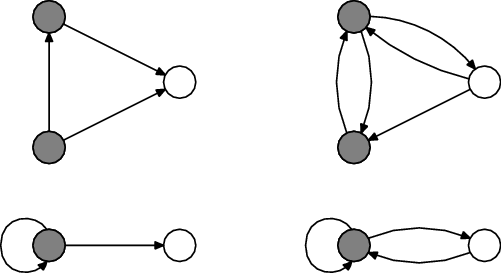
Figure 5. On the left, an example of graph morphism that is not a fibration; on the right, a fibration. Colors on the nodes are used to implicitly specify the morphisms (arcs are mapped in the only possible way).
Definition 5.
If
 $\varphi \,:\,G\to B$
is a fibration, given a vector
$\varphi \,:\,G\to B$
is a fibration, given a vector
 $\boldsymbol{{u}}$
of size
$\boldsymbol{{u}}$
of size
 $n_B$
, define its lifting along
$n_B$
, define its lifting along
 $\varphi$
as the vector
$\varphi$
as the vector
 $\boldsymbol{{u}}^\varphi$
of size
$\boldsymbol{{u}}^\varphi$
of size
 $n_G$
given by
$n_G$
given by
 \begin{equation*} \left (\boldsymbol{{u}}^\varphi \right )_i=u_{\varphi (i)}. \end{equation*}
Otherwise said,
 $\boldsymbol{{u}}^\varphi$
is the vector obtained by copying
$\boldsymbol{{u}}^\varphi$
is the vector obtained by copying
 $\boldsymbol{{u}}$
along the fibers of
$\boldsymbol{{u}}$
along the fibers of
 $\varphi$
.
$\varphi$
.
Theorem 4. (Sachs, 1966) If
 $\varphi \,:\,G\to B$
is a fibration surjective on the nodes, given a vector
$\varphi \,:\,G\to B$
is a fibration surjective on the nodes, given a vector
 $\boldsymbol{{u}}$
of size
$\boldsymbol{{u}}$
of size
 $n_B$
we have
$n_B$
we have
 \begin{equation*} \boldsymbol{{u}}^\varphi G = (\boldsymbol{{u}} B)^\varphi . \end{equation*}
In other words, one can lift and multiply by
 $G$
, or equivalently multiply by
$G$
, or equivalently multiply by
 $B$
and then lift: the base
$B$
and then lift: the base
 $B$
“summarizes” the graph
$B$
“summarizes” the graph
 $G$
well enough that the multiplication of fiberwise constant vectors by
$G$
well enough that the multiplication of fiberwise constant vectors by
 $G$
can be carried on (usually smaller)
$G$
can be carried on (usually smaller)
 $B$
. The proof of Theorem 4 is in fact immediate once one realizes that Definition 4 implies that
$B$
. The proof of Theorem 4 is in fact immediate once one realizes that Definition 4 implies that
 $\varphi$
induces a local isomorphism between the in-neighborhood of a node
$\varphi$
induces a local isomorphism between the in-neighborhood of a node
 $x$
of
$x$
of
 $G$
and the in-neighborhood of
$G$
and the in-neighborhood of
 $\varphi _N(x)$
(Boldi & Vigna, Reference Boldi and Vigna2002).
$\varphi _N(x)$
(Boldi & Vigna, Reference Boldi and Vigna2002).
Theorem 4 has the important consequence that every left eigenvector
 $\boldsymbol{{e}}$
of
$\boldsymbol{{e}}$
of
 $B$
can be lifted to a left eigenvector
$B$
can be lifted to a left eigenvector
 $\boldsymbol{{e}}^\varphi$
of
$\boldsymbol{{e}}^\varphi$
of
 $G$
, so every eigenvalue of
$G$
, so every eigenvalue of
 $B$
is an eigenvalue of
$B$
is an eigenvalue of
 $G$
, and thus, the characteristic polynomial of
$G$
, and thus, the characteristic polynomial of
 $B$
divides that of
$B$
divides that of
 $G$
(hence the name graph divisor). In our case, by the Perron–Frobenius theorem (Berman & Plemmons, Reference Berman and Plemmons1994), if
$G$
(hence the name graph divisor). In our case, by the Perron–Frobenius theorem (Berman & Plemmons, Reference Berman and Plemmons1994), if
 $B$
is strongly connected the dominant eigenvector of
$B$
is strongly connected the dominant eigenvector of
 $B$
is strictly positive, so its lifting is strictly positive, and thus (applying again the Perron–Frobenius theorem), it is the dominant eigenvector of
$B$
is strictly positive, so its lifting is strictly positive, and thus (applying again the Perron–Frobenius theorem), it is the dominant eigenvector of
 $G$
; moreover,
$G$
; moreover,
 $G$
and
$G$
and
 $B$
share the same dominant eigenvalue (and thus spectral radius).
$B$
share the same dominant eigenvalue (and thus spectral radius).
8. Back to eigenvector centrality
We now get back to eigenvector centrality: Figure 6 shows a family of total graphs
 $G_k$
depending on an integer parameter
$G_k$
depending on an integer parameter
 $k$
, and an associated family of bases
$k$
, and an associated family of bases
 $B_k$
, with fibrations defined on the nodes following the node labels, and on the arcs in the only possible way. We will show that when the edge
$B_k$
, with fibrations defined on the nodes following the node labels, and on the arcs in the only possible way. We will show that when the edge
 $0-1$
is added to the graphs (obtaining new graphs
$0-1$
is added to the graphs (obtaining new graphs
 $G^{\prime}_k$
and
$G^{\prime}_k$
and
 $B^{\prime}_k$
), all vertices labeled with
$B^{\prime}_k$
), all vertices labeled with
 $4$
, which used to have a smaller score than vertex
$4$
, which used to have a smaller score than vertex
 $1$
in
$1$
in
 $G_k$
, will become more important than vertex
$G_k$
, will become more important than vertex
 $1$
in
$1$
in
 $G^{\prime}_k$
.
$G^{\prime}_k$
.

Figure 6. The parametric counterexample graph for eigenvector centrality: when adding the edge
 $0-1$
, vertex
$0-1$
, vertex
 $1$
violates rank monotonicity (top). The
$1$
violates rank monotonicity (top). The
 $k$
vertices labeled with
$k$
vertices labeled with
 $4$
form a
$4$
form a
 $(k+1)$
-clique with vertex
$(k+1)$
-clique with vertex
 $0$
, and the
$0$
, and the
 $k$
vertices labeled with
$k$
vertices labeled with
 $6$
form a
$6$
form a
 $(k+1)$
-clique with vertices
$(k+1)$
-clique with vertices
 $2$
; finally, there is a star with
$2$
; finally, there is a star with
 $(k-1)(k-2)$
leaves around vertex
$(k-1)(k-2)$
leaves around vertex
 $1$
. Arc labels represent multiplicity. The matrix displayed is the adjacency matrix of
$1$
. Arc labels represent multiplicity. The matrix displayed is the adjacency matrix of
 $B_k$
, with the grayed entries to be set to
$B_k$
, with the grayed entries to be set to
 $1$
when
$1$
when
 $0-1$
is added to the graph. Table 2 shows a set of values for the size of the cliques and the size of the star causing vertex
$0-1$
is added to the graph. Table 2 shows a set of values for the size of the cliques and the size of the star causing vertex
 $1$
to be less important than vertex
$1$
to be less important than vertex
 $0$
.
$0$
.
The intuitive idea behind the graphs
 $G_k$
is that the new edge makes the vertices labeled with
$G_k$
is that the new edge makes the vertices labeled with
 $4$
much closer to vertex
$4$
much closer to vertex
 $1$
, a high-degree vertex; at the same time, the new edge doubles the number of paths from the vertices labeled with
$1$
, a high-degree vertex; at the same time, the new edge doubles the number of paths from the vertices labeled with
 $6$
to the vertices labeled with
$6$
to the vertices labeled with
 $4$
. The advantage for vertex
$4$
. The advantage for vertex
 $1$
is to get much closer to the vertices labeled with
$1$
is to get much closer to the vertices labeled with
 $4$
, but those have a much smaller degree. All in all, the new edge will turn out to be much more advantageous for the vertices labeled with
$4$
, but those have a much smaller degree. All in all, the new edge will turn out to be much more advantageous for the vertices labeled with
 $4$
than for vertex
$4$
than for vertex
 $1$
.
$1$
.
The fundamental property of our counterexample is that albeit
 $G_k$
is a simple undirected graph with
$G_k$
is a simple undirected graph with
 $k^2-k-6$
vertices,
$k^2-k-6$
vertices,
 $B_k$
is a general directed multigraph with seven nodes, independently of
$B_k$
is a general directed multigraph with seven nodes, independently of
 $k$
, so its adjacency matrix, shown in Figure 6, is a fixed-sized matrix containing a parameter
$k$
, so its adjacency matrix, shown in Figure 6, is a fixed-sized matrix containing a parameter
 $k$
due to the variable number of arcs. Thus, fibrations make it possible to move our proof from matrices of arbitrary size to a parametric matrix of fixed size.
$k$
due to the variable number of arcs. Thus, fibrations make it possible to move our proof from matrices of arbitrary size to a parametric matrix of fixed size.
8.1 Sturm polynomials
There is no way to compute exactly the eigenvalues and eigenvectors of
 $B_k$
. However, we will be able to control their behavior using Sturm polynomials (Rahman & Schmeisser, Reference Rahman and Schmeisser2002), a standard, powerful technique to analyze and locate real roots of polynomials.
$B_k$
. However, we will be able to control their behavior using Sturm polynomials (Rahman & Schmeisser, Reference Rahman and Schmeisser2002), a standard, powerful technique to analyze and locate real roots of polynomials.
Definition 6.
If
 $p(x)$
is a polynomial with real coefficients and
$p(x)$
is a polynomial with real coefficients and
 $p^{\prime}(x)$
its derivative, the Sturm sequence of polynomials associated with
$p^{\prime}(x)$
its derivative, the Sturm sequence of polynomials associated with
 $p(x)$
is defined by
$p(x)$
is defined by
 \begin{align*} S_0(x) &= p(x)\\ S_1(x) &= p^{\prime}(x)\\ S_{i+1}(x) &= - S_{i}(x) \bmod S_{i-1}(x)\qquad for\ i\geq 1, \end{align*}
where
 $S_{i}(x) \bmod S_{i-1}(x)$
is the remainder of the Euclidean division of
$S_{i}(x) \bmod S_{i-1}(x)$
is the remainder of the Euclidean division of
 $S_i(x)$
by
$S_i(x)$
by
 $S_{i-1}(x)$
. The sequence stops when
$S_{i-1}(x)$
. The sequence stops when
 $S_{i+1}(x)$
becomes zero, and it is long at most as the degree of
$S_{i+1}(x)$
becomes zero, and it is long at most as the degree of
 $p(x)$
.
$p(x)$
.
Given a real number
 $a$
, the number of sign variations
$a$
, the number of sign variations
 $V(a)$
of a Sturm sequence is the number of sign changes, ignoring zeros, of the sequence
$V(a)$
of a Sturm sequence is the number of sign changes, ignoring zeros, of the sequence
 $S_0(a)$
,
$S_0(a)$
,
 $S_1(a)$
,
$S_1(a)$
,
 $S_2(a)$
,
$S_2(a)$
,
 $\dots \,$
. Finally, if
$\dots \,$
. Finally, if
 $p(x)$
is squarefree (i.e., it is not divisible by the square of a nonconstant polynomial), the number of distinct roots of
$p(x)$
is squarefree (i.e., it is not divisible by the square of a nonconstant polynomial), the number of distinct roots of
 $p(x)$
in the interval
$p(x)$
in the interval
 $(a\ldotp \ldotp b]$
is
$(a\ldotp \ldotp b]$
is
 $V(a)-V(b)$
; all polynomials we will study will be squarefree.
$V(a)-V(b)$
; all polynomials we will study will be squarefree.
8.2 Bounding the dominant eigenvalue
We now discuss how to bound the dominant eigenvalue
 $\rho _k$
of
$\rho _k$
of
 $B_k$
(and thus
$B_k$
(and thus
 $G_k$
); the same results hold for the dominant eigenvalue
$G_k$
); the same results hold for the dominant eigenvalue
 $\rho^{\prime}_k\gt \rho _k$
of
$\rho^{\prime}_k\gt \rho _k$
of
 $B^{\prime}_k$
(and thus
$B^{\prime}_k$
(and thus
 $G^{\prime}_k$
). The approach we describe will be used throughout the rest of the paper.
$G^{\prime}_k$
). The approach we describe will be used throughout the rest of the paper.
Consider the characteristic polynomial of
 $B_k$
$B_k$
 \begin{equation*} p_k(\lambda ) = \det\! (1- \lambda B_k). \end{equation*}
We can compute its Sturm polynomials and evaluate them at the points
 $k+\frac 1{k^2}$
and
$k+\frac 1{k^2}$
and
 $k+\frac 3{4k}$
. This evaluation leaves us with a pair of rational functions in
$k+\frac 3{4k}$
. This evaluation leaves us with a pair of rational functions in
 $k$
for each Sturm polynomial in the sequence, and such functions have a defined sign for
$k$
for each Sturm polynomial in the sequence, and such functions have a defined sign for
 $k\to \infty$
that depends on the sign of the ratio of the leading coefficients of their numerator and denominator: in other words, for large enough
$k\to \infty$
that depends on the sign of the ratio of the leading coefficients of their numerator and denominator: in other words, for large enough
 $k$
we can count the number of zeroes of
$k$
we can count the number of zeroes of
 $p_k(\lambda )$
in the interval
$p_k(\lambda )$
in the interval
 $\big(k+\frac 1{k^2}\ldotp \ldotp k+\frac 3{4k}\big]$
, and indeed
$\big(k+\frac 1{k^2}\ldotp \ldotp k+\frac 3{4k}\big]$
, and indeed
 $p_k(\lambda )$
has exactly one zero in that interval for
$p_k(\lambda )$
has exactly one zero in that interval for
 $k\geq 24$
.
$k\geq 24$
.
If we apply the same technique to the interval
 $\left (k+\frac 3{4k}\ldotp \ldotp 2k\right ]$
, we find no zeroes. Since
$\left (k+\frac 3{4k}\ldotp \ldotp 2k\right ]$
, we find no zeroes. Since
 $2k$
is an upper bound for the dominant eigenvalue of both matrices (as it is larger than the geometric mean of indegree and outdegree of all vertices (Kwapisz, Reference Kwapisz1996, Theorem 1.(ii)), we conclude that the spectral radius
$2k$
is an upper bound for the dominant eigenvalue of both matrices (as it is larger than the geometric mean of indegree and outdegree of all vertices (Kwapisz, Reference Kwapisz1996, Theorem 1.(ii)), we conclude that the spectral radius
 $\rho _k$
of
$\rho _k$
of
 $B_k$
lies in
$B_k$
lies in
 $\left (k+\frac 1{k^2}\ldotp \ldotp k+\frac 3{4k}\right ]$
.
$\left (k+\frac 1{k^2}\ldotp \ldotp k+\frac 3{4k}\right ]$
.
8.3 Bounding the dominant eigenvector
Armed with this knowledge, we approach the study of the dominant eigenvectors of
 $B_k$
and
$B_k$
and
 $B^{\prime}_k$
. There is no way to compute them exactly: thus, we resort to the study of
$B^{\prime}_k$
. There is no way to compute them exactly: thus, we resort to the study of
 $\textbf 1(1 -\alpha B_k )^{-1}$
, because the dominant eigenvector
$\textbf 1(1 -\alpha B_k )^{-1}$
, because the dominant eigenvector
 $\boldsymbol{{e}}$
of
$\boldsymbol{{e}}$
of
 $B_k$
and
$B_k$
and
 $\boldsymbol{{e}}^{\prime}$
of
$\boldsymbol{{e}}^{\prime}$
of
 $B^{\prime}_k$
can be expressed as (Vigna, Reference Vigna2016)
$B^{\prime}_k$
can be expressed as (Vigna, Reference Vigna2016)
 \begin{align} \boldsymbol{{e}} &= \lim _{\alpha \to 1/\rho _k}\bigl (1-\alpha \rho _k\bigr )\textbf 1\bigl (1 -\alpha B_k\bigr )^{-1}. \end{align}
 \begin{align} \boldsymbol{{e}}^{\prime} &= \lim _{\alpha \to 1/\rho^{\prime}_k}\bigl (1-\alpha \rho^{\prime}_k\bigr )\textbf 1\bigl (1 -\alpha B^{\prime}_k\bigr )^{-1}. \end{align}
In fact,
 $(1 -\alpha B_k )^{-1}$
is a slightly different way (up to a constant factor) to define the resolvent of
$(1 -\alpha B_k )^{-1}$
is a slightly different way (up to a constant factor) to define the resolvent of
 $B_k$
(Dunford & Schwartz, Reference Dunford and Schwartz1988), but the formulation we use here will make it easier to apply the results we will develop in the sections on Katz’s index and PageRank.
$B_k$
(Dunford & Schwartz, Reference Dunford and Schwartz1988), but the formulation we use here will make it easier to apply the results we will develop in the sections on Katz’s index and PageRank.
While we have no way to compute exactly the eigenvectors of
 $B_k$
, we can compute symbolically
$B_k$
, we can compute symbolically
 $\textbf 1 (1 -\alpha B_k )^{-1}$
, thus obtaining for each node of
$\textbf 1 (1 -\alpha B_k )^{-1}$
, thus obtaining for each node of
 $B_k$
a rational function in
$B_k$
a rational function in
 $\alpha$
whose coefficients are polynomials in
$\alpha$
whose coefficients are polynomials in
 $k$
, and do the same for
$k$
, and do the same for
 $B^{\prime}_k$
.
$B^{\prime}_k$
.
We will be interested in comparing eigenvector centralities, that is, in proving statements (for nodes
 $x$
and
$x$
and
 $y$
of
$y$
of
 $B_k$
) of the form
$B_k$
) of the form
 \begin{equation*} \frac {e_x}{e_y}=\lim _{\alpha \to 1/\rho _k}\frac {\left [\bigl (1-\alpha \rho _k\bigr )\textbf 1\bigl (1 -\alpha B_k\bigr )^{-1}\right ]_x}{\left [ \bigl (1-\alpha \rho _k\bigr )\textbf 1\bigl (1 -\alpha B_k\bigr )^{-1}\right ]_y}\gt 1. \end{equation*}
However,
 \begin{equation*} \frac {e_x}{e_y}=\lim _{\alpha \to 1/\rho _k}\frac {\left [\textbf 1\bigl (1 -\alpha B_k\bigr )^{-1}\right ]_x}{\left [ \textbf 1\bigl (1 -\alpha B_k\bigr )^{-1}\right ]_y} =\lim _{\alpha \to 1/\rho _k}\frac {\left [\textbf 1\cdot \textrm {adj}({1-\alpha B_k})\right ]_x}{\left [\textbf 1\cdot \textrm {adj}({1-\alpha B_k})\right ]_y} =\frac {\left [\textbf 1\cdot \textrm {adj}({1- B_k/\rho _k})\right ]_x}{\left [\textbf 1\cdot \textrm {adj}({1- B_k/\rho _k})\right ]_y}, \end{equation*}
where we used the fact that the inverse is the adjugate matrix (Gantmacher, Reference Gantmacher1980) divided by the determinant
 \begin{equation*} \textrm {adj}({1-\alpha B_k})=\bigl (1 -\alpha B_k\bigr )^{-1}\cdot \det\! (1 -\alpha B_k). \end{equation*}
The final substitution can be performed safely because the column-sums of the adjugate must be nonzero in a neighborhood of
 $\rho _k$
, or the limits (1) would not be finite and positive. The advantage is that the entries of
$\rho _k$
, or the limits (1) would not be finite and positive. The advantage is that the entries of
 $\textrm{adj}({1-\alpha B_k})$
are just polynomials. The same considerations hold for
$\textrm{adj}({1-\alpha B_k})$
are just polynomials. The same considerations hold for
 $B^{\prime}_k$
.
$B^{\prime}_k$
.
We thus define, for every node
 $x$
,
$x$
,
 \begin{align*} \textrm{pre}_\alpha (x)&= \left [\textbf 1\cdot \textrm{adj}({1 -\alpha B_k})\right ]_x\\[4pt] \textrm{post}_\alpha (x)&= \left [\textbf 1\cdot \textrm{adj}({1 -\alpha B^{\prime}_k})\right ]_x. \end{align*}
For example,
 \begin{align} \textrm{pre}_\alpha (0) &= ({-}2k^3 + 7k^2 - 7k + 2)\alpha ^6 + (2k^2 - 7k + 5)\alpha ^5 + (2k^3 - 6k^2 + 6k)\alpha ^4\\
&\qquad \qquad \qquad \qquad \qquad + (k^3 - 5k^2 + 9k - 7)\alpha ^3 + ({-}k^2 + k - 3)\alpha ^2 + ({-}k + 2)\alpha + 1. \end{align}
\begin{align} \textrm{pre}_\alpha (0) &= ({-}2k^3 + 7k^2 - 7k + 2)\alpha ^6 + (2k^2 - 7k + 5)\alpha ^5 + (2k^3 - 6k^2 + 6k)\alpha ^4\\
&\qquad \qquad \qquad \qquad \qquad + (k^3 - 5k^2 + 9k - 7)\alpha ^3 + ({-}k^2 + k - 3)\alpha ^2 + ({-}k + 2)\alpha + 1. \end{align}
Note that in the adjacency matrix of
 $B_k$
just three rows contain
$B_k$
just three rows contain
 $k$
: as a consequence, the degree in
$k$
: as a consequence, the degree in
 $k$
of the coefficients of the polynomials in
$k$
of the coefficients of the polynomials in
 $\alpha$
is at most three.
$\alpha$
is at most three.
Since
 $k+\frac 3{4k}\gt \rho _k$
, we start by showing that
$k+\frac 3{4k}\gt \rho _k$
, we start by showing that
 \begin{equation*} \textrm {pre}_{1\big/\left (k+\frac 3{4k}\right )}(1)\gt \textrm {pre}_{1\big/\left (k+\frac 3{4k}\right )}(4) \end{equation*}
and once again, since we are dealing with rational functions in
 $k$
, for enough large
$k$
, for enough large
 $k$
the difference
$k$
the difference
 \begin{equation*} \textrm {pre}_{1\big/\left (k+\frac 3{4k}\right )}(1)-\textrm {pre}_{1\big/\left (k+\frac 3{4k}\right )}(4) \end{equation*}
has a constant sign: in particular, for
 $k\geq 53$
it is positive. The same analysis, however, shows that
$k\geq 53$
it is positive. The same analysis, however, shows that
 \begin{equation*} \textrm {post}_{1\big/\left (k+\frac 3{4k}\right )}(1) \lt \textrm {post}_{1\big/\left (k+\frac 3{4k}\right )}(4) \end{equation*}
when
 $k\geq 3$
.
$k\geq 3$
.
We are now going to extend our inequalities to a range comprising
 $1/\rho _k$
. If we consider the Sturm polynomials (in
$1/\rho _k$
. If we consider the Sturm polynomials (in
 $\alpha$
) of
$\alpha$
) of
 \begin{equation*} \textrm {pre}_\alpha (1)- \textrm {pre}_\alpha (4),\end{equation*}
we find no zero between
 $\alpha = 1\big/\left (k+\frac 3{4k}\right ) \lt 1/ \rho _k$
and
$\alpha = 1\big/\left (k+\frac 3{4k}\right ) \lt 1/ \rho _k$
and
 $\alpha = 1\big/\left (k+\frac 1{k^2}\right ) \gt 1/ \rho _k$
for
$\alpha = 1\big/\left (k+\frac 1{k^2}\right ) \gt 1/ \rho _k$
for
 $k\geq 53$
. Hence, for
$k\geq 53$
. Hence, for
 $1\big/\left (k+\frac 3{4k}\right )\lt \alpha \leq 1\big/\left (k+\frac 1{k^2}\right )$
 \begin{equation*} \textrm {pre}_\alpha (1)\gt \textrm {pre}_\alpha (4), \end{equation*}
so, in particular,
 \begin{equation*} \textrm {pre}_{1/\rho _k}(1)\gt \textrm {pre}_{1/\rho _k}(4), \end{equation*}
showing that the eigenvector centrality of node
 $1$
is larger than that of node
$1$
is larger than that of node
 $4$
for
$4$
for
 $k\geq 53$
. A similar analysis for
$k\geq 53$
. A similar analysis for
 $\textrm{post}$
shows that
$\textrm{post}$
shows that
 \begin{equation*} \textrm {post}_{1/\rho^{\prime}_k}(1)\lt \textrm {post}_{1/\rho^{\prime}_k}(4) \end{equation*}
for
 $k\geq 1$
. Thus, in the graph
$k\geq 1$
. Thus, in the graph
 $G_k$
the addition of the edge
$G_k$
the addition of the edge
 $0-1$
causes vertex
$0-1$
causes vertex
 $1$
to violate rank monotonicity. Further analysis of the same kind on the remaining nodes show that only the vertices labeled with
$1$
to violate rank monotonicity. Further analysis of the same kind on the remaining nodes show that only the vertices labeled with
 $4$
change their importance relatively to vertex
$4$
change their importance relatively to vertex
 $1$
, which implies that vertex
$1$
, which implies that vertex
 $1$
is demoted by
$1$
is demoted by
 $k$
positions. Finally, studying the polynomial
$k$
positions. Finally, studying the polynomial
 $\textrm{pre}_\alpha (1)-\textrm{pre}_\alpha (0)$
it is easy to see that in our example vertex
$\textrm{pre}_\alpha (1)-\textrm{pre}_\alpha (0)$
it is easy to see that in our example vertex
 $1$
is more important than vertex
$1$
is more important than vertex
 $0$
for
$0$
for
 $k\geq 54$
.
$k\geq 54$
.
While all the previous discussions are valid for
 $k\geq 54$
, numerical computations show that the result indeed extends to all
$k\geq 54$
, numerical computations show that the result indeed extends to all
 $k\geq 7$
. Hence:
$k\geq 7$
. Hence:
Theorem 5.
Eigenvector centrality is not rank monotone (top violation) on the graphs
 $G_k$
of Figure
6
for
$G_k$
of Figure
6
for
 $k\geq 7$
.
$k\geq 7$
.
By gaging accurately the size of the star around
 $1$
, it is possible to find also bottom violations of rank monotonicity. We have tabulated the first few values of
$1$
, it is possible to find also bottom violations of rank monotonicity. We have tabulated the first few values of
 $k$
for which there is a suitable star, and we show them in Table 2: we conjecture that there is a function of
$k$
for which there is a suitable star, and we show them in Table 2: we conjecture that there is a function of
 $k$
of order
$k$
of order
 $\Theta (k^2)$
which gives a correct real value for
$\Theta (k^2)$
which gives a correct real value for
 $s$
, and examples emerge when such value is very close to an integer.
$s$
, and examples emerge when such value is very close to an integer.


9. Seeley’s index
A natural variant of eigenvector centrality is Seeley’s index (Seeley, Reference Seeley1949), the steady state of the (uniform) random walk on the graph; for more details, see Boldi & Vigna (Reference Boldi and Vigna2014). The situation here is quite different: it is a well-known fact that if the graph is connected the only possible steady-state probability of vertex
 $x$
is simply
$x$
is simply
 $d(x)/2m$
, where
$d(x)/2m$
, where
 $d(x)$
is the degree of
$d(x)$
is the degree of
 $x$
—essentially, the centrality of a vertex is just its
$x$
—essentially, the centrality of a vertex is just its
 $\ell _1$
-normalized degree. We will use this definition on all graphs, albeit in the general case it does not give the only possible steady state. As a consequence:
$\ell _1$
-normalized degree. We will use this definition on all graphs, albeit in the general case it does not give the only possible steady state. As a consequence:
Theorem 6.
Seeley’s index (defined as
 $\ell _1$
-normalized degree) is strictly rank monotone on undirected graphs.
$\ell _1$
-normalized degree) is strictly rank monotone on undirected graphs.
The situation is almost the same for score monotonicity:
Theorem 7.
Seeley’s index (defined as
 $\ell _1$
-normalized degree) is score monotone on undirected graphs, except in the case of a graph formed by a star graph and one or more additional isolated vertices.
$\ell _1$
-normalized degree) is score monotone on undirected graphs, except in the case of a graph formed by a star graph and one or more additional isolated vertices.
Proof.
When we add an edge between
 $x$
and
$x$
and
 $y$
in a graph with
$y$
in a graph with
 $m$
edges, the score of
$m$
edges, the score of
 $x$
changes from
$x$
changes from
 $d(x)/2m$
to
$d(x)/2m$
to
 $(d(x)+1)/(2m+2)$
. If we require
$(d(x)+1)/(2m+2)$
. If we require
 \begin{equation*} \frac {d(x)+1}{2m+2}\gt \frac {d(x)}{2m} \end{equation*}
we obtain
 $d(x)\lt m$
. Since obviously
$d(x)\lt m$
. Since obviously
 $d(x)\leq m$
, the condition is always true except when
$d(x)\leq m$
, the condition is always true except when
 $d(x)=m$
, which corresponds to the case of a disconnected graph formed by a star graph and by additional isolated vertices. Indeed, in that case adding an edge between an isolated vertex and the center of the star will not change the score of the center.
$d(x)=m$
, which corresponds to the case of a disconnected graph formed by a star graph and by additional isolated vertices. Indeed, in that case adding an edge between an isolated vertex and the center of the star will not change the score of the center.
Theorem 7 is a general characterization of score monotonicity of Seeley’s index, under the assumption that its values are given by
 $\ell _1$
-normalized degree. Since we aim at providing connected counterexamples only, in Table 1 we do not use the negative part of Theorem 7, marking Seeley’s index as score monotone. Furthermore, note that while in general Seeley’s index on unconnected graphs may have several definitions,
$\ell _1$
-normalized degree. Since we aim at providing connected counterexamples only, in Table 1 we do not use the negative part of Theorem 7, marking Seeley’s index as score monotone. Furthermore, note that while in general Seeley’s index on unconnected graphs may have several definitions,
 $\ell _1$
-normalized degree yields the only possible steady state even in the case of a graph formed by a nontrivial connected component plus isolated vertices.
$\ell _1$
-normalized degree yields the only possible steady state even in the case of a graph formed by a nontrivial connected component plus isolated vertices.
10. Interlude: Graph fibrations and damped spectral rankings
The key observation used to build the counterexample for eigenvector centrality was Theorem 4, stating that lifting of vectors commutes with matrix multiplication.
The theorem is true also for weighted graphs, as long as the fibration preserves weights and adjacency matrices are defined by adding the weights of all arcs between two nodes. An interesting consequence of this fact is the following:
Theorem 8.
[Boldi et al., Reference Boldi, Lonati, Santini and Vigna2006
] Let
 $G$
and
$G$
and
 $B$
be weighted graphs, and
$B$
be weighted graphs, and
 $\varphi \,:\,G\to B$
be a surjective weight-preserving fibration; then, given a (row) vector
$\varphi \,:\,G\to B$
be a surjective weight-preserving fibration; then, given a (row) vector
 $\boldsymbol{{v}}$
of size
$\boldsymbol{{v}}$
of size
 $n_B$
we have
$n_B$
we have
 \begin{equation*} \boldsymbol{{v}}^\varphi (1-\alpha G)^{-1} = \bigl (\boldsymbol{{v}} (1-\alpha B)^{-1}\bigr )^\varphi . \end{equation*}
The proof is simple:
 \begin{align*} \boldsymbol{{v}}^\varphi (1-\alpha G)^{-1} & = \boldsymbol{{v}}^\varphi \sum _{i=0}^\infty (\alpha G)^i = \sum _{i=0}^\infty \boldsymbol{{v}}^\varphi (\alpha G)^i \\& = \sum _{i=0}^\infty \bigl (\boldsymbol{{v}} (\alpha B)^i\bigr )^\varphi = \left(\boldsymbol{{v}}\sum _{i=0}^\infty (\alpha B)^i\right)^\varphi = \bigl (\boldsymbol{{v}} (1-\alpha B)^{-1}\bigr )^\varphi . \end{align*}
Theorem 8 makes it possible to apply the techniques we used for eigenvector centrality to general damped spectral rankings, as defined in Vigna (Reference Vigna2016), of which both Katz’s index and PageRank are special instances. Both centralities can be defined, up to a constant multiplying factor, as
 \begin{equation*} \boldsymbol{{v}} (1-\alpha M)^{-1} \end{equation*}
for suitable preference vector
 $\boldsymbol{{v}}$
and for a matrix
$\boldsymbol{{v}}$
and for a matrix
 $M$
derived from the adjacency matrix of the graph.
$M$
derived from the adjacency matrix of the graph.
11. Katz’s index
Recall that Katz’s index (Katz, Reference Katz1953) is defined as
 \begin{equation*} \textbf 1\sum _{i=0}^\infty \alpha ^i G^i = \textbf 1(1-\alpha G)^{-1}, \end{equation*}
where
 $0\leq \alpha \lt 1/\rho (G)$
(here,
$0\leq \alpha \lt 1/\rho (G)$
(here,
 $\rho (G)$
is the spectral radius of
$\rho (G)$
is the spectral radius of
 $G$
). It is trivially score monotone, but we will prove that it is not rank monotone.
$G$
). It is trivially score monotone, but we will prove that it is not rank monotone.
First of all, we note that if
 $\alpha$
is small enough Katz’s index will be strictly rank monotone:
$\alpha$
is small enough Katz’s index will be strictly rank monotone:
Theorem 9.
Let
 $G$
be a graph and
$G$
be a graph and
 $\rho$
its spectral radius. Then, there is an
$\rho$
its spectral radius. Then, there is an
 $\bar \alpha \lt 1/\rho$
such that for
$\bar \alpha \lt 1/\rho$
such that for
 $\alpha \leq \bar \alpha$
Katz’s index is strictly rank monotone on
$\alpha \leq \bar \alpha$
Katz’s index is strictly rank monotone on
 $G$
.
$G$
.
Proof. We remark that
 \begin{equation*} \textbf 1\sum _{i=0}^\infty \alpha ^i G^i = \textbf 1 + \alpha \textbf 1G + \alpha ^2 \textbf 1 G^2\sum _{i=0}^\infty \alpha ^i G^i. \end{equation*}
The relative node importance in
 $\textbf 1 + \alpha \textbf 1G$
is exactly that defined by degree, and score differences are
$\textbf 1 + \alpha \textbf 1G$
is exactly that defined by degree, and score differences are
 $O(\alpha )$
for
$O(\alpha )$
for
 $\alpha \to 0$
. However,
$\alpha \to 0$
. However,
 \begin{equation*} \Biggl \|\alpha ^2\textbf 1 G^2 \sum _{i=0}^\infty \alpha ^iG^i\Biggr \|_\infty \leq \alpha ^2\bigl \|G^2\bigr \|_\infty \Biggl \|\sum _{i=0}^\infty \alpha ^i G^i\Biggr \|_\infty, \end{equation*}
and given any
 $0\lt \alpha^{\prime}\lt 1/\rho _k$
for
$0\lt \alpha^{\prime}\lt 1/\rho _k$
for
 $\alpha \leq \alpha^{\prime}$
the last expression is
$\alpha \leq \alpha^{\prime}$
the last expression is
 $O (\alpha ^2 )$
for
$O (\alpha ^2 )$
for
 $\alpha \to 0$
. Thus, there is an
$\alpha \to 0$
. Thus, there is an
 $\alpha _G$
such that, for
$\alpha _G$
such that, for
 $\alpha \leq \alpha _G$
, the relative importance of a node of
$\alpha \leq \alpha _G$
, the relative importance of a node of
 $G$
is that defined by its degree. If we minimize over all such
$G$
is that defined by its degree. If we minimize over all such
 $\alpha$
’s for all graphs obtained by adding an edge to
$\alpha$
’s for all graphs obtained by adding an edge to
 $G$
, we obtain the value
$G$
, we obtain the value
 $\bar \alpha$
of the statement.
$\bar \alpha$
of the statement.
On the other hand, we are now going to provide an example on which rank monotonicity is not satisfied when we go sufficiently close to
 $1/\rho$
. We can use the same counterexample as for eigenvector centrality (Figure 6): in view of Theorem 8, the analysis performed in Section 8 already shows that Katz’s index is not rank monotone on
$1/\rho$
. We can use the same counterexample as for eigenvector centrality (Figure 6): in view of Theorem 8, the analysis performed in Section 8 already shows that Katz’s index is not rank monotone on
 $G_k$
for sufficiently large
$G_k$
for sufficiently large
 $k$
and for all
$k$
and for all
 \begin{equation*} \alpha \in \biggl [\frac 1{k+\frac 3{4k}}\ldotp \ldotp \frac 1{\rho^{\prime}_k}\biggr ). \end{equation*}
In other words,
Theorem 10.
Let
 $\rho^{\prime}_k$
be the spectral radius of the graph
$\rho^{\prime}_k$
be the spectral radius of the graph
 $G^{\prime}_k$
in Figure
6. For
$G^{\prime}_k$
in Figure
6. For
 $k\geq 54$
, there exists some
$k\geq 54$
, there exists some
 $\nu _k\lt \frac 1{k+\frac 3{4k}}$
such that Katz’s index is not rank monotone (top violation) on
$\nu _k\lt \frac 1{k+\frac 3{4k}}$
such that Katz’s index is not rank monotone (top violation) on
 $G_k$
for all
$G_k$
for all
 $\alpha \in \left (\nu _k\ldotp \ldotp \frac 1{\rho^{\prime}_k}\right )$
.
$\alpha \in \left (\nu _k\ldotp \ldotp \frac 1{\rho^{\prime}_k}\right )$
.
Note that the theorem above claims that the violation happens in a left neighborhood of the upper bound of
 $\alpha$
; moreover, on the left we can get as close as desired to
$\alpha$
; moreover, on the left we can get as close as desired to
 $0$
given a suitable
$0$
given a suitable
 $k$
. This is the best possible scenario, in view of Theorem 9. Also our considerations about demotion in Section 8 transfer immediately to the present setting.
$k$
. This is the best possible scenario, in view of Theorem 9. Also our considerations about demotion in Section 8 transfer immediately to the present setting.
Further analysis by Sturm polynomials in the interval
 $\left (\frac 1{k+\frac 1k}\ldotp \ldotp \frac 1{k+\frac 3{4k}}\right ]$
shows the following:
$\left (\frac 1{k+\frac 1k}\ldotp \ldotp \frac 1{k+\frac 3{4k}}\right ]$
shows the following:
-
the relative importance of node
 $1$
and node
$4$
in
$\textrm{pre}_\alpha ({-})$
flips (node
$4$
is more important than node
$1$
at the beginning of the interval and then becomes less important, after some value of
$\alpha$
, say
$\alpha^{\prime}$
);
$1$
and node
$4$
in
$\textrm{pre}_\alpha ({-})$
flips (node
$4$
is more important than node
$1$
at the beginning of the interval and then becomes less important, after some value of
$\alpha$
, say
$\alpha^{\prime}$
); -
the relative importance of node
$0$
and node
$1$
in
$\textrm{pre}_\alpha ({-})$
flips (node
$0$
is more important than node
$1$
at the beginning of the interval and then becomes less important, after some value of
$\alpha$
, say
$\alpha^{\prime\prime}$
); -
$\textrm{pre}_\alpha (1)-\textrm{pre}_\alpha (4)$
always dominates
$\textrm{pre}_\alpha (1)-\textrm{pre}_\alpha (0)$
.


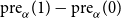
The latter observation implies
 $\alpha^{\prime}\lt \alpha^{\prime\prime}=\nu _k$
, in the notation of Theorem 10; since the relative importance of node
$\alpha^{\prime}\lt \alpha^{\prime\prime}=\nu _k$
, in the notation of Theorem 10; since the relative importance of node
 $1$
and node
$1$
and node
 $4$
remains the same in
$4$
remains the same in
 $\textrm{post}_\alpha ({-})$
(node
$\textrm{post}_\alpha ({-})$
(node
 $4$
is always more important than node
$4$
is always more important than node
 $1$
in the interval after the addition of the edge), in the interval
$1$
in the interval after the addition of the edge), in the interval
 $ (\alpha^{\prime}\ldotp \ldotp \nu _k )$
, we can observe a bottom violation of rank monotonicity.
$ (\alpha^{\prime}\ldotp \ldotp \nu _k )$
, we can observe a bottom violation of rank monotonicity.
Moreover, the interval
 $(\alpha^{\prime}\ldotp \ldotp \nu _k)$
gets closer to the upper bound
$(\alpha^{\prime}\ldotp \ldotp \nu _k)$
gets closer to the upper bound
 $\frac 1{\rho^{\prime}_k}\gt \nu _k$
as
$\frac 1{\rho^{\prime}_k}\gt \nu _k$
as
 $k$
gets larger:
$k$
gets larger:
 \begin{equation*} \frac {\frac 1{\rho^{\prime}_k} - \alpha^{\prime}}{\frac 1{\rho^{\prime}_k}}\leq \frac {\frac 1{\rho^{\prime}_k} - \frac 1{k+\frac 1k}}{\frac 1{\rho^{\prime}_k}} = 1-\frac {\rho^{\prime}_k}{k+\frac 1k}\leq 1-\frac {k+\frac 1{k^2}}{k+\frac 1k}\to 0 \quad \text {for $k\to \infty $}. \end{equation*}
Theorem 11.
For every
 $k$
, there is an interval of values of
$k$
, there is an interval of values of
 $\alpha$
contained in
$\alpha$
contained in
 $\left (\frac 1{k+\frac 1k}\ldotp \ldotp \frac 1{k+\frac 3{4k}}\right ]$
in which Katz’s index is not rank monotone (bottom violation). The interval gets arbitrarily close to
$\left (\frac 1{k+\frac 1k}\ldotp \ldotp \frac 1{k+\frac 3{4k}}\right ]$
in which Katz’s index is not rank monotone (bottom violation). The interval gets arbitrarily close to
 $\frac 1{\rho^{\prime}_k}$
as
$\frac 1{\rho^{\prime}_k}$
as
 $k\to \infty$
.
$k\to \infty$
.
As a final consideration, there is another range of validity of Theorem 10: if we further analyze with Sturm polynomials the relative importance of node
 $1$
and node
$1$
and node
 $4$
in the interval
$4$
in the interval
 $\left (\frac 1{k+\frac 2k}\ldotp \ldotp \frac 1{k+\frac 3{4k}}\right ]$
, we find two sign changes in
$\left (\frac 1{k+\frac 2k}\ldotp \ldotp \frac 1{k+\frac 3{4k}}\right ]$
, we find two sign changes in
 $\textrm{pre}_\alpha (1)- \textrm{pre}_\alpha (4)$
, two sign changes in
$\textrm{pre}_\alpha (1)- \textrm{pre}_\alpha (4)$
, two sign changes in
 $\textrm{pre}_\alpha (1)- \textrm{pre}_\alpha (0)$
, and zero sign changes in
$\textrm{pre}_\alpha (1)- \textrm{pre}_\alpha (0)$
, and zero sign changes in
 $\textrm{post}_\alpha (1)- \textrm{post}_\alpha (4)$
: thus, there is an interval comprising
$\textrm{post}_\alpha (1)- \textrm{post}_\alpha (4)$
: thus, there is an interval comprising
 $\frac 1{k+\frac 2k}$
in which the violation of rank monotonicity happens again. Also in this interval,
$\frac 1{k+\frac 2k}$
in which the violation of rank monotonicity happens again. Also in this interval,
 $\textrm{pre}_\alpha (1)-\textrm{pre}_\alpha (4)$
always dominates
$\textrm{pre}_\alpha (1)-\textrm{pre}_\alpha (4)$
always dominates
 $\textrm{pre}_\alpha (1)-\textrm{pre}_\alpha (0)$
; hence, we have both top violations and bottom violations; it is also immediate to show demotion. Figure 7 summarizes graphically the results proved in this section.
$\textrm{pre}_\alpha (1)-\textrm{pre}_\alpha (0)$
; hence, we have both top violations and bottom violations; it is also immediate to show demotion. Figure 7 summarizes graphically the results proved in this section.
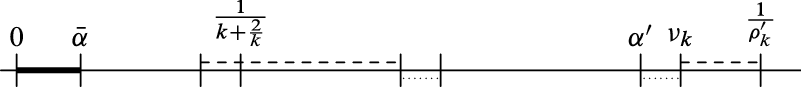
Figure 7. A graphical summarization of the results about Katz’s index proved in Section 11. Dashed lines (dotted lines, resp.) represent intervals of values of
 $\alpha$
, in which we proved top (bottom, resp.) violations of rank monotonicity (Theorems 10 and 11). The thick interval represents a region where rank monotonicity is guaranteed (Theorem 9).
$\alpha$
, in which we proved top (bottom, resp.) violations of rank monotonicity (Theorems 10 and 11). The thick interval represents a region where rank monotonicity is guaranteed (Theorem 9).
12. PageRank
PageRank (Page et al., Reference Page, Brin, Motwani and Winograd1998) can be defined as
 \begin{equation*} (1-\alpha )\boldsymbol{{v}}\sum _{i=0}^\infty \alpha ^i\bar G^i = (1-\alpha ) \boldsymbol{{v}}(1-\alpha \bar G)^{-1}, \end{equation*}
where
 $\alpha \in [0\ldotp \ldotp 1)$
is the damping factor,
$\alpha \in [0\ldotp \ldotp 1)$
is the damping factor,
 $\boldsymbol{{v}}$
is a non-negative preference vector with unit
$\boldsymbol{{v}}$
is a non-negative preference vector with unit
 $\ell _1$
-norm, and
$\ell _1$
-norm, and
 $\bar G$
is the row-normalized versionFootnote
5
of
$\bar G$
is the row-normalized versionFootnote
5
of
 $G$
; that is,
$G$
; that is,
 $\bar G$
is just the (adjacency matrix of the) weighted version of
$\bar G$
is just the (adjacency matrix of the) weighted version of
 $G$
defined by letting
$G$
defined by letting
 $w(a)=1/\sum _{x\in N_G}G_{s_G(a)\, x}$
. Hence, if you have a weighted graph
$w(a)=1/\sum _{x\in N_G}G_{s_G(a)\, x}$
. Hence, if you have a weighted graph
 $B$
, a weight-preserving fibration
$B$
, a weight-preserving fibration
 $\varphi \,:\, \bar G \to B$
that is surjective on the nodes, and a vector
$\varphi \,:\, \bar G \to B$
that is surjective on the nodes, and a vector
 $\boldsymbol{{u}}$
of size
$\boldsymbol{{u}}$
of size
 $n_B$
such that
$n_B$
such that
 $\boldsymbol{{u}}^\varphi$
has unit
$\boldsymbol{{u}}^\varphi$
has unit
 $\ell _1$
-norm, you can deduce from Theorem 8 that
$\ell _1$
-norm, you can deduce from Theorem 8 that
 \begin{equation} (1-\alpha ) \boldsymbol{{u}}^\varphi (1-\alpha \bar G)^{-1}=\left ( (1-\alpha ) \boldsymbol{{u}} (1-\alpha B)^{-1}\right )^\varphi . \end{equation}
On the left-hand side you have the actual PageRank of
 $G$
for a preference vector that is fiberwise constant; on the right-hand side you have a damped spectral ranking of
$G$
for a preference vector that is fiberwise constant; on the right-hand side you have a damped spectral ranking of
 $B$
. Note that
$B$
. Note that
 $B$
is not necessarily row-stochastic, and
$B$
is not necessarily row-stochastic, and
 $\boldsymbol{{u}}$
has not unit
$\boldsymbol{{u}}$
has not unit
 $\ell _1$
-norm, so technically the right-hand side of the equation in Theorem 8 is not PageRank anymore.
$\ell _1$
-norm, so technically the right-hand side of the equation in Theorem 8 is not PageRank anymore.
We first observe that
Theorem 12.
Given an undirected connected graph
 $G$
, there is a value of
$G$
, there is a value of
 $\alpha$
for which PageRank is score monotone and strictly rank monotone on
$\alpha$
for which PageRank is score monotone and strictly rank monotone on
 $G$
.
$G$
.
Proof.
We know that for
 $\alpha \to 1$
, PageRank tends to Seeley’s index (Boldi et al., Reference Boldi, Santini and Vigna2005), which under our connectedness hypothesis is just
$\alpha \to 1$
, PageRank tends to Seeley’s index (Boldi et al., Reference Boldi, Santini and Vigna2005), which under our connectedness hypothesis is just
 $\ell _1$
-normalized degree. Since Seeley’s index is strictly rank monotone (Theorem 6), for each non-adjacent pair of vertices
$\ell _1$
-normalized degree. Since Seeley’s index is strictly rank monotone (Theorem 6), for each non-adjacent pair of vertices
 $x$
and
$x$
and
 $y$
there is a value
$y$
there is a value
 $\alpha _{xy}$
such that for
$\alpha _{xy}$
such that for
 $\alpha \geq \alpha _{xy}$
adding the edge
$\alpha \geq \alpha _{xy}$
adding the edge
 $x-y$
is strictly rank monotone. The proof is completed by taking
$x-y$
is strictly rank monotone. The proof is completed by taking
 $\alpha$
larger than all
$\alpha$
larger than all
 $\alpha _{xy}$
’s. The result for score monotonicity is similar, using Theorem 7.
$\alpha _{xy}$
’s. The result for score monotonicity is similar, using Theorem 7.
It is interesting to remark that this result is dual to Theorem 9: Katz’s index is approximated by degree for values of the damping factor close to the lower bound (zero), whereas PageRank is approximated by degree for values of the damping factor close to the upper bound (one). Note that the part about score monotonicity of Theorem 12 has a flavor similar to statement (2) of Theorem 4.1 in Avrachenkov & Litvak (Reference Avrachenkov and Litvak2006).
On the other hand, we will now show that for every possible value of the damping factor
 $\alpha$
there is a graph on which PageRank is neither rank nor score monotone. Our proof strategy will be identical to the one we used for Katz’s index, except that now we expect our example to satisfy rank monotonicity when
$\alpha$
there is a graph on which PageRank is neither rank nor score monotone. Our proof strategy will be identical to the one we used for Katz’s index, except that now we expect our example to satisfy rank monotonicity when
 $\alpha$
is close to its upper bound, instead of its lower bound, because of Theorem 12.
$\alpha$
is close to its upper bound, instead of its lower bound, because of Theorem 12.
In Figure 8, we show a family of total graphs
 $G_k$
depending on an integer parameter
$G_k$
depending on an integer parameter
 $k$
, and an associated family of bases
$k$
, and an associated family of bases
 $B_k$
, with fibrations defined on the nodes following the node labels, and on the arcs in the only possible way.Footnote
6
Weights are defined by normalizing the adjacency matrix of
$B_k$
, with fibrations defined on the nodes following the node labels, and on the arcs in the only possible way.Footnote
6
Weights are defined by normalizing the adjacency matrix of
 $G_k$
and then using the fibration to transfer the weights on the arcs
$G_k$
and then using the fibration to transfer the weights on the arcs
 $B_k$
(it is easy to see that no conflict arises when multiple arcs of
$B_k$
(it is easy to see that no conflict arises when multiple arcs of
 $G_k$
are mapped to the same arc of
$G_k$
are mapped to the same arc of
 $B_k$
). As usual,
$B_k$
). As usual,
 $G^{\prime}_k$
and
$G^{\prime}_k$
and
 $B^{\prime}_k$
are the same graphs with the additional edge
$B^{\prime}_k$
are the same graphs with the additional edge
 $0-1$
.
$0-1$
.

Figure 8. A parametric counterexample graph for PageRank: when adding the edge
 $0-1$
, vertex
$0-1$
, vertex
 $1$
violates score and rank monotonicity (bottom violation). The
$1$
violates score and rank monotonicity (bottom violation). The
 $k$
vertices labeled with
$k$
vertices labeled with
 $4$
form a
$4$
form a
 $(k+1)$
-clique with vertex
$(k+1)$
-clique with vertex
 $3$
, and the
$3$
, and the
 $k-1$
vertices labeled with
$k-1$
vertices labeled with
 $8$
form a
$8$
form a
 $(k+1)$
-clique with vertices
$(k+1)$
-clique with vertices
 $0$
and
$0$
and
 $7$
. Arc labels represent multiplicity; weights are induced by the uniform distribution on the upper graph. The matrices displayed are the adjacency matrix of
$7$
. Arc labels represent multiplicity; weights are induced by the uniform distribution on the upper graph. The matrices displayed are the adjacency matrix of
 $B_k$
and
$B_k$
and
 $B^{\prime}_k$
; differently from Figure 6, we show them both explicitly to highlight how the addition of the new edge influences row normalization.
$B^{\prime}_k$
; differently from Figure 6, we show them both explicitly to highlight how the addition of the new edge influences row normalization.
The basic intuition behind the graphs
 $G_k$
is that when you connect a high-degree vertex
$G_k$
is that when you connect a high-degree vertex
 $x$
with a low-degree vertex
$x$
with a low-degree vertex
 $y$
,
$y$
,
 $y$
will pass to
$y$
will pass to
 $x$
a much larger fraction of its score than in the opposite direction. This phenomenon is caused by the stochastic normalization of the adjacency matrix: the arc from
$x$
a much larger fraction of its score than in the opposite direction. This phenomenon is caused by the stochastic normalization of the adjacency matrix: the arc from
 $x$
to
$x$
to
 $y$
will have a low coefficient, due to the high degree of
$y$
will have a low coefficient, due to the high degree of
 $x$
, whereas the arc from
$x$
, whereas the arc from
 $y$
to
$y$
to
 $x$
will have a high coefficient, due to the low degree of
$x$
will have a high coefficient, due to the low degree of
 $y$
.
$y$
.
While
 $G_k$
has
$G_k$
has
 $2k+6$
vertices,
$2k+6$
vertices,
 $B_k$
has
$B_k$
has
 $9$
vertices, independently of
$9$
vertices, independently of
 $k$
, and thus, its PageRank can be computed analytically as rational functions of
$k$
, and thus, its PageRank can be computed analytically as rational functions of
 $\alpha$
whose coefficients are rational functions in
$\alpha$
whose coefficients are rational functions in
 $k$
(since the number of arcs of each
$k$
(since the number of arcs of each
 $B_k$
is different).
$B_k$
is different).
We thus define, for every node
 $x$
,
$x$
,
 \begin{align*} \textrm{pre}_\alpha (x)&= \left [(1-\alpha )\textbf 1\bigl (1 -\alpha B_k\bigr )^{-1}\right ]_x\\[4pt] \textrm{post}_\alpha (x)&= \left [(1-\alpha )\textbf 1\bigl (1 -\alpha B^{\prime}_k\bigr )^{-1}\right ]_x. \end{align*}
Note when discussing score monotonicity, we cannot use the adjugate matrix to simplify our computations, as we did in Section 8, but we can use without loss of generality an arbitrary constant vector as preference vector. When discussing rank monotonicity, however, we will switch silently to the adjugate (because the denominator cannot change its sign anywhere in
 $[0\ldotp \ldotp 1)$
).
$[0\ldotp \ldotp 1)$
).
For example,
 \begin{equation*} \textrm {post}_\alpha (1)= \frac {\frac {2 k^{2} - 6 k + 4}{k^{2} - 6 k + 4} \alpha ^{5} + \frac {-14 k^{2} + 12 k + 4}{k^{2} - 6 k + 4} \alpha ^{4} +\cdots + \frac {6 k^{4} + 6 k^{3} - 24 k^{2} - 24 k}{k^{2} - 6 k + 4} \alpha + \frac {-4 k^{4} - 12 k^{3} - 8 k^{2}}{k^{2} - 6 k + 4}} {\alpha ^{5} + \frac {-2 k^{3} - 10 k^{2} + 12 k + 4}{k^{2} - 6 k + 4} \alpha ^{4} + \cdots + \frac {4 k^{4} + 4 k^{3} - 20 k^{2} - 24 k}{k^{2} - 6 k + 4} \alpha + \frac {-4 k^{4} - 12 k^{3} - 8 k^{2}}{k^{2} - 6 k + 4}}, \end{equation*}
where we omitted part of the terms for lack of space. Once again, in the adjacency matrix of
 $B_k$
just four rows contain
$B_k$
just four rows contain
 $k$
: as a consequence, the degree in
$k$
: as a consequence, the degree in
 $k$
of numerators and denominators of coefficients of the rational functions in
$k$
of numerators and denominators of coefficients of the rational functions in
 $\alpha$
is at most four.
$\alpha$
is at most four.
12.1 Score monotonicity
We start by considering node
 $1$
: evaluating
$1$
: evaluating
 $\textrm{post}_\alpha (1)-\textrm{pre}_\alpha (1)$
in
$\textrm{post}_\alpha (1)-\textrm{pre}_\alpha (1)$
in
 $\alpha =2/3$
, we obtain a negative value for
$\alpha =2/3$
, we obtain a negative value for
 $k\geq 11$
, showing there is a value of
$k\geq 11$
, showing there is a value of
 $\alpha$
for which node
$\alpha$
for which node
 $1$
violates score monotonicity. Then, we use again Sturm polynomials to show that for
$1$
violates score monotonicity. Then, we use again Sturm polynomials to show that for
 $k\geq 13$
the numerator of
$k\geq 13$
the numerator of
 $\textrm{post}_\alpha (1)-\textrm{pre}_\alpha (1)$
never changes its sign in
$\textrm{post}_\alpha (1)-\textrm{pre}_\alpha (1)$
never changes its sign in
 $ (a_k\ldotp \ldotp b_k ]$
, where
$ (a_k\ldotp \ldotp b_k ]$
, where
 \begin{equation*} a_k = \frac 23 - \frac {2k}{3k+ 100} \lt \frac 23 \lt \frac 23+\frac {k}{3k+100} = b_k, \end{equation*}
while the denominator of
 $\textrm{post}_\alpha (1)-\textrm{pre}_\alpha (1)$
cannot have zeros in
$\textrm{post}_\alpha (1)-\textrm{pre}_\alpha (1)$
cannot have zeros in
 $[0\ldotp \ldotp 1)$
. The interval
$[0\ldotp \ldotp 1)$
. The interval
 $ (a_k\ldotp \ldotp b_k ]$
approaches
$ (a_k\ldotp \ldotp b_k ]$
approaches
 $(0\ldotp \ldotp 1]$
as
$(0\ldotp \ldotp 1]$
as
 $k$
grows, so we conclude that the interval of values of
$k$
grows, so we conclude that the interval of values of
 $\alpha$
for which the score of node
$\alpha$
for which the score of node
 $1$
decreases reaches the whole unit interval as
$1$
decreases reaches the whole unit interval as
 $k$
grows.
$k$
grows.
Finally, by studying (as in the case of Katz’s index) the polynomial
 $\textrm{pre}_\alpha (1)-\textrm{pre}_\alpha (0)$
it is easy to see that in our example node
$\textrm{pre}_\alpha (1)-\textrm{pre}_\alpha (0)$
it is easy to see that in our example node
 $0$
is always more important than node
$0$
is always more important than node
 $1$
as long as
$1$
as long as
 $k\geq 1$
.
$k\geq 1$
.
Theorem 13.
For every value of
 $\alpha \in (0\ldotp \ldotp 1)$
, for sufficiently large
$\alpha \in (0\ldotp \ldotp 1)$
, for sufficiently large
 $k$
PageRank with damping factor
$k$
PageRank with damping factor
 $\alpha$
is not score monotone (bottom violation) on the graphs
$\alpha$
is not score monotone (bottom violation) on the graphs
 $G_k$
of Figure
8.
$G_k$
of Figure
8.
It is also interesting to count the sign changes of
 $\textrm{post}_\alpha (1)-\textrm{pre}_\alpha (1)$
in
$\textrm{post}_\alpha (1)-\textrm{pre}_\alpha (1)$
in
 $ (0\ldotp \ldotp a_k ]$
(one) and
$ (0\ldotp \ldotp a_k ]$
(one) and
 $ (b_k\ldotp \ldotp 1 )$
(one), as they describe the behavior of the score change for limiting values: initially, the score increases; then, it starts to decrease somewhere before
$ (b_k\ldotp \ldotp 1 )$
(one), as they describe the behavior of the score change for limiting values: initially, the score increases; then, it starts to decrease somewhere before
 $a_k$
and stops decreasing somewhere after
$a_k$
and stops decreasing somewhere after
 $b_k$
, as expected from Theorem 12.
$b_k$
, as expected from Theorem 12.
12.2 Rank monotonicity
We now use the same example to prove the lack of rank monotonicity. In this case, we study in a similar way
 $\textrm{pre}_\alpha (1)-\textrm{pre}_\alpha (5)$
, which is positive in
$\textrm{pre}_\alpha (1)-\textrm{pre}_\alpha (5)$
, which is positive in
 $\alpha =2/3$
if
$\alpha =2/3$
if
 $k\geq 13$
. To extend our results about rank monotonicity to every
$k\geq 13$
. To extend our results about rank monotonicity to every
 $\alpha$
, we use again Sturm polynomials to show that the numerator of
$\alpha$
, we use again Sturm polynomials to show that the numerator of
 $\textrm{pre}_\alpha (1)-\textrm{pre}_\alpha (5)$
never changes its sign in
$\textrm{pre}_\alpha (1)-\textrm{pre}_\alpha (5)$
never changes its sign in
 $ (a_k\ldotp \ldotp b_k ]$
for
$ (a_k\ldotp \ldotp b_k ]$
for
 $k\geq 14$
.
$k\geq 14$
.
Again, it is interesting to count the sign changes of
 $p(\alpha )$
in
$p(\alpha )$
in
 $(0\ldotp \ldotp a_k]$
(one) and
$(0\ldotp \ldotp a_k]$
(one) and
 $(b_k\ldotp \ldotp 1)$
(one): initially, node
$(b_k\ldotp \ldotp 1)$
(one): initially, node
 $1$
has a smaller PageRank than node
$1$
has a smaller PageRank than node
 $5$
; then, somewhere before
$5$
; then, somewhere before
 $a_k$
, node
$a_k$
, node
 $1$
starts having a larger PageRank than
$1$
starts having a larger PageRank than
 $5$
; somewhere after
$5$
; somewhere after
 $b_k$
, we return to the initial condition, as expected from Theorem 12.
$b_k$
, we return to the initial condition, as expected from Theorem 12.
Finally, we study
 $\textrm{post}_\alpha (1)-\textrm{post}_\alpha (5)$
which is negative in
$\textrm{post}_\alpha (1)-\textrm{post}_\alpha (5)$
which is negative in
 $\alpha =2/3$
and again has no sign changes in
$\alpha =2/3$
and again has no sign changes in
 $ (a_k\ldotp \ldotp b_k ]$
for
$ (a_k\ldotp \ldotp b_k ]$
for
 $k\geq 5$
. More precisely, we study
$k\geq 5$
. More precisely, we study
 $p(\alpha )$
, where
$p(\alpha )$
, where
 $\textrm{post}_\alpha (1)-\textrm{post}_\alpha (5) = (1-\alpha )^2p(\alpha )$
, as
$\textrm{post}_\alpha (1)-\textrm{post}_\alpha (5) = (1-\alpha )^2p(\alpha )$
, as
 $\textrm{post}_\alpha (1)-\textrm{post}_\alpha (5)$
is not squarefree, but
$\textrm{post}_\alpha (1)-\textrm{post}_\alpha (5)$
is not squarefree, but
 $p(\alpha )$
is.
$p(\alpha )$
is.
In this case, there are two sign changes in
 $(0\ldotp \ldotp a_k]$
and no sign change in
$(0\ldotp \ldotp a_k]$
and no sign change in
 $(b_k\ldotp \ldotp 1)$
, so initially, node
$(b_k\ldotp \ldotp 1)$
, so initially, node
 $1$
is less important than node
$1$
is less important than node
 $5$
; then, in an interval of values before
$5$
; then, in an interval of values before
 $a_k$
it is more important; then, it starts to be again less important before
$a_k$
it is more important; then, it starts to be again less important before
 $a_k$
; and it becomes as important as node
$a_k$
; and it becomes as important as node
 $5$
only in the limit for
$5$
only in the limit for
 $\alpha \to 1$
.
$\alpha \to 1$
.
Theorem 14.
For every value of
 $\alpha \in (0\ldotp \ldotp 1)$
, for sufficiently large
$\alpha \in (0\ldotp \ldotp 1)$
, for sufficiently large
 $k$
PageRank with damping factor
$k$
PageRank with damping factor
 $\alpha$
is not rank monotone (bottom violation) on the graphs
$\alpha$
is not rank monotone (bottom violation) on the graphs
 $G_k$
of Figure
8.
$G_k$
of Figure
8.
Recall that in Boldi et al. (Reference Boldi, Luongo and Vigna2017), PageRank was proven to be both score and (strictly) rank monotone for all directed graphs and all
 $\alpha \in [0\ldotp \ldotp 1)$
, given that the preference vector is positive: comparing those results with Theorems 13 and 14, we see once more that in the undirected case the behavior is radically different.
$\alpha \in [0\ldotp \ldotp 1)$
, given that the preference vector is positive: comparing those results with Theorems 13 and 14, we see once more that in the undirected case the behavior is radically different.
For sufficiently large
 $k$
, almost all nodes are more important (i.e., have larger PageRank score) than node
$k$
, almost all nodes are more important (i.e., have larger PageRank score) than node
 $1$
both before and after edge addition, with the only exception of nodes
$1$
both before and after edge addition, with the only exception of nodes
 $5$
and
$5$
and
 $6$
: as we said, node
$6$
: as we said, node
 $5$
is less important than node
$5$
is less important than node
 $1$
before but more important after the edge addition, whereas node
$1$
before but more important after the edge addition, whereas node
 $6$
is also less important than node
$6$
is also less important than node
 $1$
before and becomes as important as node
$1$
before and becomes as important as node
 $1$
after the edge addition (as node
$1$
after the edge addition (as node
 $6$
and node
$6$
and node
 $1$
become equivalent modulo an automorphism). As a result, node
$1$
become equivalent modulo an automorphism). As a result, node
 $1$
is demoted.
$1$
is demoted.

Figure 9. A parametric counterexample graph for PageRank: when adding the edge
 $0-1$
, vertex
$0-1$
, vertex
 $0$
violates score and rank monotonicity (top violation). There is a star with
$0$
violates score and rank monotonicity (top violation). There is a star with
 $k$
leaves around vertex
$k$
leaves around vertex
 $0$
, a star with
$0$
, a star with
 $k$
leaves around vertex
$k$
leaves around vertex
 $4$
, and the
$4$
, and the
 $k$
vertices labeled with
$k$
vertices labeled with
 $6$
form a
$6$
form a
 $(k+2)$
-clique with vertices
$(k+2)$
-clique with vertices
 $1$
and
$1$
and
 $2$
. Arc labels represent multiplicity; weights are induced by the uniform distribution on the upper graph.
$2$
. Arc labels represent multiplicity; weights are induced by the uniform distribution on the upper graph.
Finally, we provide in Figure 9 a counterexample in which the more important node violates rank monotonicity. In this case, the intuition is that we connect two nodes with the same degree but different scores. As in the previous case, the counterexample works for any chosen
 $\alpha$
, up to an appropriate choice of the parameter
$\alpha$
, up to an appropriate choice of the parameter
 $k$
. The proof follows the same line of attack, and detailed computations can be found in the Sage worksheets. The main difference is that the relevant interval
$k$
. The proof follows the same line of attack, and detailed computations can be found in the Sage worksheets. The main difference is that the relevant interval
 $ (a_k\ldotp \ldotp b_k ]$
is now
$ (a_k\ldotp \ldotp b_k ]$
is now
 \begin{equation*} a_k = \frac 23-\frac {2\sqrt k}{3\sqrt k+10}\lt \alpha \leq \frac 23 + \frac k{3k+1} = b_k. \end{equation*}
Theorem 15.
For every value of
 $\alpha \in (0\ldotp \ldotp 1)$
, for sufficiently large
$\alpha \in (0\ldotp \ldotp 1)$
, for sufficiently large
 $k$
PageRank with damping factor
$k$
PageRank with damping factor
 $\alpha$
is neither score nor rank monotone (top violation) on the graphs
$\alpha$
is neither score nor rank monotone (top violation) on the graphs
 $G_k$
of Figure
9.
$G_k$
of Figure
9.
12.3 Anecdotal evidence: PageRank on the IMDB
To show that our results are not only theoretical, we provide a few interesting anecdotal examples from the PageRank scores (
 $\alpha =0.85$
) of the Hollywood co-starship graph, whose vertices are actors/actresses in the Internet Movie Database, with an edge connecting them if played in the same movie. In particular, we used the hollywood-2011 dataset from the Laboratory for Web Algorithmics,Footnote
7
which contains approximately two million vertices and
$\alpha =0.85$
) of the Hollywood co-starship graph, whose vertices are actors/actresses in the Internet Movie Database, with an edge connecting them if played in the same movie. In particular, we used the hollywood-2011 dataset from the Laboratory for Web Algorithmics,Footnote
7
which contains approximately two million vertices and
 $230$
million edges.
$230$
million edges.
To generate our examples, we picked two actors either at random, or considering the top
 1/10,000
of the actors of the graph in PageRank order and the bottom quartile, looking for a collaboration that would hurt either actor (or both).Footnote
8
About
1/10,000
of the actors of the graph in PageRank order and the bottom quartile, looking for a collaboration that would hurt either actor (or both).Footnote
8
About
 $4$
% of our samples yielded a violation of monotonicity, and in Table 3 we report a few funny examples.
$4$
% of our samples yielded a violation of monotonicity, and in Table 3 we report a few funny examples.
Table 3. A few examples of violations of score monotonicity and rank monotonicity in the Hollywood co-starship graph hollywood-2011. If we add an edge between the actors in the first and second column, the first actor has a score increase, the second actor has a score decrease, and the actors in the third column, which were less important than the second actor, become more important after the edge addition. The first three examples are bottom violations, whereas the last one is a top violation
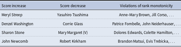
The first three cases are bottom violations: it is the less-known actor that loses score (and rank) by the collaboration with the star, and not the other way round, as it happens also in the counterexample of Figure 8. In the last case, instead, we have a top violation: a collaboration would damage the more important vertex, like in the counterexample of Figure 9. We found no case in which both actors would be hurt by the collaboration, and it is in fact an open problem whether this situation can happen.
13. Conclusions
We have studied score and rank monotonicity on undirected graphs for some popular notions of centrality. Our results show that except for Seeley’s index (on connected graphs), there are always cases in which rank monotonicity does not hold, and in the case of Katz’s index and PageRank, we can find range of values of the parameters where the violation occurs; moreover, some centralities are also not score monotone. We provide examples of both top and bottom violations to highlight that even the knowledge of whether one is the more important or less important node is insufficient to decide whether the new edge will be beneficial. A possible direction for future research is to show that top and bottom violations cannot happen at the same time; that is, that the new edge is beneficial for at least one endpoint.
This lack of monotonicity is opposite to that we observed in the directed case, and it can also be seen in real-world graphs (at least for PageRank). It is interesting to note that even centrality indices that were designed for undirected graphs (e.g., closeness) are not rank monotone in the undirected case (even under a connectedness assumption). Our results show that common knowledge and intuitions about the behavior of centrality measures in the directed case cannot be applied to the undirected case.
Competing interests
None.


 Open access