


1 INTRODUCTION
1.1. Scientific goals of KISS
The Antarctic plateau is one of the best sites on Earth for infrared (IR) and submillimetre astronomical observations (Lawrence et al. Reference Lawrence2006; Ji Yang et al. Reference Yang2010). There is an opportunity now to exploit this scientifically by deploying to Kunlun Station (Dome A) (Yuan et al. Reference Yuan2015) an IR camera for the AST3-3 wide field telescope. Location at Kunlun Station offers the supreme advantage of the whole southern sky available for continuous study for the duration of the Antarctic winter every year. The Antarctic K DARK 2.4 μm passband is a unique low background window in the IR. The Kunlun Infrared Sky Survey (KISS) is the first deep and wide K-band survey, and plays a role as a pathfinder for future large Antarctic telescopes, such as KDUST (Zhao et al. Reference Zhao2011).
AST3-3 is the third telescope in the AST3 series. Recent results from AST3-1 are reported by Li, Fu, & Liu (Reference Li, Fu and Liu2015). With its high IR sensitivity, AST3-3 science will emphasise opportunities in the time domain where longer wavelength measurements are particularly advantageous, such as the following:
-
• supernovae and the equation of state;
-
• reverberation mapping and the physics of AGN;
-
• Gamma-Ray Burster follow up;
-
• the Cosmic IR Background;
-
• terminal phases of red giants (Miras);
-
• dynamics and variability in star formation;
-
• discovery of exo-planets (esp. brown dwarfs & hot jupiters).
In this paper, we consider optimisation of the KISS K DARK filter to maximise the signal-to-noise ratio (SNR) achievable with this site and instrument. Similar considerations for another exceptional site, Mauna Kea Observatory, have been discussed (Simons & Tokunaga Reference Simons and Tokunaga2002). We outline the design of the telescope and camera in Section 2 (leaving the details for a further paper), the Dome A environment in Section 3, the optimisation algorithm in Section 4, and then draw our conclusions.
1.2. History of K dark
The first suggestion that an exceedingly dark window might exist in the IR portion of the spectrum, where the background sky brightness could be very much less than at temperate sites, was made by Harper (Reference Harper1990). This laid the foundations for the development of IR capability at the then fledgling Center for Astrophysical Research in Antarctica (CARA) Dark Sector observatory at the South Pole.
Harper realised that, at the typical –60°C winter time temperatures occurring at the South Pole, the thermal background in the K-band (i.e. from 2.0–2.4μm) would fall dramatically from the flux at temperate sites, being on the Wien side of the blackbody peak of the sky emission spectrum. Furthermore, between 2.27–2.45 μm there were no known OH airglow lines. Thus, in this narrower band the background flux could be two orders of magnitude lower than at the best temperate sites, such as Mauna Kea.
From the latter site, observations in K-band are often undertaken in the short portion of the band (i.e. λ~ < 2.3 μm), where the emission is dominated by OH airglow, in order to avoid the steeply rising thermal contribution. In contrast, Harper proposed that from the South Pole sensitivities could be greatly improved by building a telescope that made measurements from 2.27–2.45 μm, though he did not give this band a name. He even suggested that the observations might be limited by the zodiacal light. This is also near its minimum value in this band, between scattered sunlight by dust in the Ecliptic to shorter wavelengths, and emission from dust rising to the thermal IR. The gains were quantified in calculations conducted by Lubin (Reference Lubin1988) for a Masters thesis at the University of Chicago; for instance, for measurements made by equivalent-sized telescopes at the South Pole and Mauna Kea, they found that the limiting magnitude may be 2.9 mag fainter at Pole.
The science case for working in this window was then explored (Burton et al. 1993, Burton et al. 1994), as part of an extensive examination of the potential for Antarctic observatories across a wide range of the photon and particle energies. These authors modelled the performance of an Antarctic 2.5-m telescope across the near- and mid-IR bands, as well as the then-planned 8 m-class telescopes on Mauna Kea (and possible ones in Australia and Antarctica). These were benchmarked in comparison with the 3.9-m Anglo Australian Telescope (AAT). They also took into account the hypothesised ‘super-seeing’ on the Antarctic plateau (Gillingham Reference Gillingham1993). The authors called the 2.27–2.45 μm band K +, and found that an Antarctic 2.5-m telescope should be 3.2–3.7 mags more sensitive than the AAT for point source photometry (the range dependent on the assumptions made), and even 1.2–1.7 mags. more sensitive than a Mauna Kea 8-m telescope. However, since for some continuum investigations, the precise wavelength of measurement is not critical, they also compared the results to K′ measurements (i.e. 2.0–2.3 μm, without the thermal longwave end of K-band), finding that there would still be a 0.4 mag gain over a Mauna Kea 8 m.
While these predictions were impressive, they lacked site data quantifying the level of the background sky emission in order to demonstrate their validity, instead relying on model values. Two experiments were then conducted by CARA at the South Pole to measure these fluxes. One used the 60-cm SPIREX telescope, equipped with a 1–2.5 μm imaging spectrometer (the GRIM) (Nguyen et al. Reference Nguyen1996). The other used the former 1–5 μm single element photometer/spectrometer from the AAT (the IRPS) (Ashley et al. Reference Ashley1996), staring at the sky with a tilt mirror through an effective 4° beam. SPIREX had a specially optimised filter centred at 2.36 μm and running between 2.29 and 2.43 μm, which they named K DARK—the first use of this nomenclature. SPIREX found the average value of the zenith sky flux in K DARK to be 162 ± 67 μJy arcsec− 2, in contrast to ~ 4 000 μJy arcsec− 2 at Mauna Kea. The IRPS was able to obtain a spectrum of the emission with a resolution of R = 100, finding a broad minimum in sky brightness between 2.30–2.45 μm, and a flux level ranging from 50 to 250 μJy arcsec− 2. Integrated over the SPIREX K DARK bandpass, the IRPS obtained a mean flux of 180 ± 60 μJy arcsec− 2, ranging from 60 to 320 μJy arcsec− 2. While exceptionally low, these sky fluxes were still about an order of magnitude higher than originally predicted by Harper (Harper Reference Harper1990). Using the measured sky fluxes, the sensitivity gain in the K DARK band between a 2.5-m telescope at the Pole compared to the AAT was then calculated to be a factor of ~ 50 (Burton Reference Burton1996).
A more extended analysis of a full winter season of IRPS data was then undertaken (Phillips et al. Reference Phillips1999). Between 2.35–2.45 μm, the sky brightness dropped to as low as 50 μJy arcsec− 2, and ranged as high as 200 μJy arcsec2 in good conditions. A typical value is 100 μJy arcsec− 2 = 17 Vega mags arcsec− 2. No evidence of any auroral contribution to the emission was found. The lowest background levels were reached once the Sun drops more than 10° below the horizon, when it is no longer able to illuminate the airglow layer (which is at altitudes of 80–100 km). However, the lowest flux levels were still about twice those expected for a 10% emissive atmosphere at –40°C (i.e. as is often found at the top of the inversion layer). Phillips et al. concluded that the residual emission is probably airglow in origin.
The last IR site testing measurements to have been made in Antarctica come from the Near Infrared Sky Monitor (NISM) instrument, which was designed as a low-powered version of the IRPS, operating on a power budget of just 10W (Lawrence et al. Reference Lawrence2002). While intended ultimately for deployment to the high plateau, the only measurements made with the NISM were at South Pole. There was a single filter designed for measuring the K DARK flux (λcent = 2.379 μm Δλ = 0.226 μm, though with a small thermal leak which complicated the data analysis). Consistent flux levels were found with the earlier measurements, with a median sky value of ~ 120 μJy arcsec− 2.
The IR fluxes obtained with these three instruments at South Pole, together with measurements of the superb optical seeing above the surface boundary layer made at Dome C (Lawrence et al. Reference Lawrence, Ashley, Tokovinin and Travouillon2004), formed the basis for the sensitivity calculations made in extensive science cases (Burton, Storey, & Ashley Reference Burton, Storey and Ashley2001; Burton et al. Reference Burton2005; Lawrence et al. Reference Lawrence2009a; Lawrence et al. Reference Lawrence2009b; Lawrence et al. Reference Lawrence2009c) for IR telescopes proposed for Dome C. All these science cases suffered, however, from the lack of any direct measurement of actual sky fluxes from the high plateau.
1.3. Current NISM experiment
NISM is the first instrument to measure the IR sky flux from the high plateau of Antarctica. It was installed at the start of the 2015 season at Ridge A at an elevation of 4 040 m. Ridge A is 150 km from Dome A, which is the highest point on the plateau. NISM measures the sky flux using a single pixel InSb diode detector with a cold band-pass filter, which is sensitive to the K DARK window at 2.38 ± 0.08 μm (Bingham & Ashley Reference Bingham and Ashley2014).
The NISM detector is pointed at an angled mirror which makes a full 360° rotation in elevation once every 10 s, sweeping the beam across the sky with a 4° field-of-view. In one rotation, NISM observes the sky, the ground, and a blackbody. The blackbody is a copper cone which is kept at typically 30° above the ambient temperature, and acts as a reference flux to calibrate the instrument. A platinum resistance thermometer measures the blackbody temperature to an absolute accuracy of better than 0.5°C. Further information on NISM can be found in Freeman et al. (in preparation).
As these results are not yet available, for the purposes of the present study we will employ the best presently available models and measurements, and allow for several scenarios. Just which of these is most appropriate should be clarified relatively soon with the publication of the NISM results.
1.4. Motivation: optimising the filter
To maximise the science yield over the five year KISS survey mission, a key initial design criterion is optimisation of the filter bandpass. The following sections contain detailed descriptions of the thermal and atmospheric factors relevant to the camera design, our simulation methodology, and finally resultant best-case filters spanning a range of assumptions about the Dome A environment.
2 TELESCOPE AND CAMERA
2.1. Thermal design of the KISS camera
For the AST3-3 telescope, Narcissus mirrors (Gillingham Reference Gillingham2002) were first proposed to control extraneous thermal backgrounds. As part of the design effort, the thermal emission from telescope and IR camera was investigated more closely, and we examined different thermal control options by either adding a narcissus mirror or a controlling pad behind the telescope secondary mirror. It became clear that a full cold-stop within the camera is a feasible, less risky, and economical solution for this kind of survey telescope.
2.2. Emissivity of telescope and camera
The AST3-3 IR camera is designed for operation at Dome A, Antarctica, where the ambient temperature is very low during winter. A major source of background radiation setting the noise floor for observation of faint astronomical sources is blackbody thermal emission from the atmosphere and the telescope. These are mostly composed of atmospheric emissivity, emission from telescope mirrors and structures in the beam (such as warm windows), surfaces within the cryostat, as well as thermal emission from within instrument that is scattered onto the detector. Due to the site’s extremely low sky emission (compared to a temperate site), it becomes necessary to perform a rigorous examination of the thermal self-emission (TSE) from the telescope and instrument, as these could play a substantial role in setting the background.
Figure 1 shows a model of AST3-3 KISS camera. It includes a transparent entrance window of diameter of 500 mm with an Indium Tin Oxide thin film deposited at the front for de-frosting and an aspheric surface at the back for correcting optical aberrations. A primary and a folding secondary mirror form an f/3.76 intermediate focus before the IR camera re-imaging optics. A field stop is placed here to limit stray light entering the IR camera. The KISS camera includes a flat vacuum window to separate the telescope body from the dewar, and a folding mirror to make the system more compact. The IR re-imaging optics includes four lenses and one filter as well as a cold pupil stop preventing thermal emission from warm camera surfaces arriving on the detector. The final focal ratio of the system is f/5.36, while the plate scale of the IR camera is 1.38 arcsec pixel−1 (size: 18 μm). The image quality of the system will be about 1.36 arcsec providing a match to expectations for episodes of better seeing.
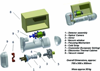
Figure 1. KISS camera design. Light enters the window (4), is reflected from the flat (3) and focusses through the camera (2) on the detector (1).
TSE from structures within telescope and instrument can be calculated from three quantities: (1) the absolute temperature T which determines the spectrum of blackbody radiation from the Planck function B λ(T), (2) the emissivity ε(λ) of each component which determines the fraction of blackbody radiation’s contribution, and (3) the solid angle which is subtended to the detector plane. To estimate the emissivity of optical components, Kirchhoff’s law was used. For mirrors, emissivity can be calculated as: ε = 1 − R, where R is the measured mirror reflectance. The emissivity of an optical lens can be estimated from its absorption as ε = absorption.
A comprehensive inventory of the properties of opto-mechanical elements making up the telescope and camera was compiled—key elements such as the tube and baffle of the telescope and KISS camera are painted black with an emissivity of 0.95, while the Indium Tin Oxide coating has emissivity of 0.13.
Using the FREDFootnote 1 optical engineering simulation package, the solid angle from each object was calculated so that the TSE received by detector can be accumulated.
Because the AST-3 telescope was not designed at the outset as an IR optimised instrument, the thermal radiation reaching the detector is actually a factor of a few worse than an idealised design (wherein only unavoidable flux from mirrors and transmissive optics in the optical path contributes). Mitigating against this, however, is the fact that the telescope enclosure itself is in such a cold environment that the TSE remains lower than the sky contribution. The solid angle for each object is then examined using a Matlab program and by varying the temperature of each object according to its position within the telescope, the total TSE can be obtained. Figure 2 shows the calculated thermal emission radiance from the system, when the telescope ambient temperature is 210 K, and the IR camera optics chamber is 150 K, and the detector is 77 K.
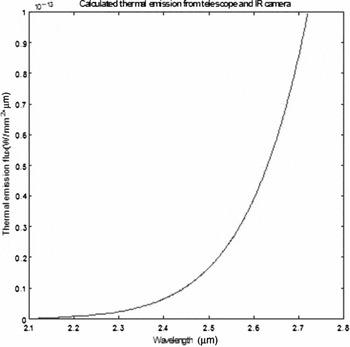
Figure 2. Calculated thermal self-emission on the detector plane.
3 THE ATMOSPHERE AND ENVIRONMENT
3.1. Temperature range of Dome A and ground level seeing
There are, as yet, no direct measurements of the night time seeing at Dome A. However, and as discussed in Burton et al. (Reference Burton2010), we may anticipate the value for the seeing at Dome A based on measurements of meteorological parameters, and by comparison with the levels determined at other high plateau sites, in particular, the South Pole and Dome A.
There is a narrow and intense boundary layer above Dome A. Measurements of its height have been made using a sonic radar (a SNODAR) (Bonner et al. Reference Bonner2010), yielding a median value of 13.9 m, and a 25% quartile of just 9.7 m. For a telescope placed above this boundary layer, it is anticipated that it will experience only the free atmosphere seeing. The value should be at least as good as that measured from Dome C (which is 900 m lower in elevation); here, the median value was found to be 0.27 arcsec in V–band (Lawrence et al. Reference Lawrence, Ashley, Tokovinin and Travouillon2004). The boundary layer at Dome A is also much thinner than at the South Pole, where it is ~ 200 m (Marks Reference Marks2002), and about half that at Dome C (23–27 m) (Aristidi et al. Reference Aristidi2009), so facilitating the ease of raising a telescope above it.
Within the boundary layer, there is a strong temperature gradient. Analysis of temperature measurements made from a weather tower at Dome A (Hu et al. Reference Hu2014) show that typically this is 15°C between the ice surface of the top of the boundary layer; i.e. a temperature gradient of ~ 1°Cm−1. The gradient is particularly intense close to the surface; for instance, the mean temperatures measured by Hu et al. at 0, 2, and 4 m above the ice are -60^, -54^, and -52^C, respectively.
There is also a considerable range in the temperature at Dome A. While hourly variations are generally less than 1°C (and there are no diurnal variations in winter), over week long periods the temperature can vary by up to 20°C. For instance, over the winter period, and at a height 4 m above the ice, the temperature ranges from − 70° to − 45°C. Within the boundary layer, the contribution to the seeing is considerable. At any given height close to the ice, the seeing is also variable, depending particularly on whether it happens to be above the boundary layer at the time. We estimate the boundary layer seeing at Dome A by comparison with measurements made at other high plateau sites.
At the South Pole, this layer contributes typically 1.5 arcsec at Pole in V-band (Marks et al. Reference Marks, Vernin, Azouit, Briggs, Burton, Ashley and Manigault1996, Reference Marks, Vernin, Azouit, Manigault and Clevelin1999) and 1.1 arcsec at 2.4 μm (Marks Reference Marks2002). The distribution of seeing measurements close to the ice surface at Dome C has a bi-modal distribution (Aristidi et al. Reference Aristidi2009); at 8-m elevation, the two peaks are at 0.4 arcsec and 1.6 arcsec. The former corresponds to times when the top of boundary layer drops below 8 m and occurs about 20% of the time. The latter is the more normal condition, with the mean boundary layer at Dome C being determined by Aristidi et al. to be between 23–27 m. At Dome F, daytime measurements made from an instrument placed 11 m above the ice (Okita et al. Reference Okita, Ichikawa, Ashley, Takato and Motoyama2013) found the seeing to sometimes drop below 0.2 arcsec at V-band. This would then correspond to the free-atmosphere value, with the monitor then above the boundary layer. A median value was found to be 0.54 arcsec, with a tail extending up to 3 arcsec. These include the contribution from the free atmosphere as well as the boundary layer, whose median height is estimated to be 18 m.
We anticipate a similar situation to also occur at Dome A, compressed into the ~ 15-m depth of the boundary layer. The boundary layer seeing would then be ~ 1 arcsec at K dark, and when the top boundary layer drops below the height of a telescope, the free atmosphere seeing of better than 0.3 arcsec would be obtained. Direct measurements of the seeing at Dome A are desirable.
3.2. Atmospheric transmission
Unfortunately, dedicated measurements of the atmospheric transmission spanning the near-IR are not available for the Dome A site. Summaries of the status of Antarctic observational campaigns have been given (Burton Reference Burton1998).
However, a sophisticated treatment employing the atmospheric modelling programme MODTRAN to model the observed sky spectrum at the South Pole from the near-IR to the submillimetre has been used (Hidas et al. Reference Hidas, Burton, Chamberlain and Storey2000). The model incorporates more than a dozen atomic and molecular species, as well as the effects of aerosols (but does not incorporate a contribution from airglow). Extracted below in Figure 3 are models of the polar atmospheric transmission over the two micron region. These span a range of values for the total precipitable water content with the ‘mid’ model corresponding to 164 μm, while ‘wet’ and ‘dry’ are 324 μm and 82 μm, respectively.
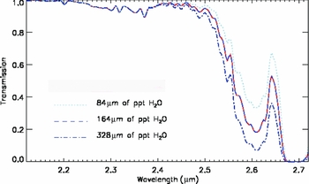
Figure 3. Curves of South Pole atmospheric transmission taken from Hidas et al. (Reference Hidas, Burton, Chamberlain and Storey2000), with varying assumptions about the atmospheric water content. The three lines are for precipitable water columns of 84, 164, and 328 μm.
3.3. Atmospheric OH
One inescapable source of IR background for observations from ground-based observatories is the vibration–rotation spectrum of the OH molecule. The first overtone band is centred at 1.6 μm, but the higher vibrational states emit in lines that extend into the K-band window. Highly useful data are available (Rousselot et al. Reference Rousselot, Lidman, Cuby, Moreels and Monnet2000), shown here as Figures 4 and 5. Provided the short wavelength cutoff λ1~ > 2.3 μm, the background variability due to airglow will be minimised.
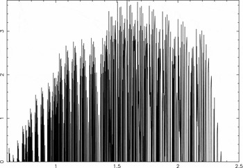
Figure 4. Intensity of OH lines in the catalogue of Rousselot et al. (log scale).
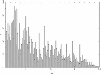
Figure 5. Number of lines in the catalogue. The horizontal axis is wavelength in this and the previous figure.
3.4. Thermal background emissivity and the atmosphere
Measurements of the thermal sky background are available (Ashley et al. Reference Ashley1996; Phillips et al. Reference Phillips1999). These pertain to the South Pole, and conditions on the plateau are expected to be significantly darker. The measured sky brightness from these two sources has been plotted in Figure 6. Note that these two sources yield somewhat discrepant data, and in particular, both the position and the shape of the K DARK region around 2.4 μm differing. For the purposes of optimisation of the KISS survey bandpass in later sections, we have adopted the Ashley et al. (Reference Ashley1996) curves (in which the 2.4 μm dark region plays a more accentuated role). For the purposes of optimising the shape of the K DARK bandpass we make use of the sky spectrum presented in Ashley et al. (Reference Ashley1996) as opposed to that in Phillips et al. (Reference Phillips1999). The former represents the best conditions at South Pole, whereas the latter the average conditions. We expect it to provide a better model for the colder and clearer conditions of Dome A compared to South Pole.
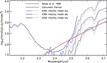
Figure 6. Measured infrared sky brightness from the South Pole taken from Ashley et al. (Reference Ashley1996). Thermal self-emission from the instrumentation, as well as simple emissivity models assuming a cold, dry dome-A atmosphere are also presented (further details in the text). Note that Figure 1 of Phillips et al. (Reference Phillips1999) provides additional observations of the sky from the South Pole, however these data appear to have an error in their wavelength calibration, and so are not used here.
Also overplotted in Figure 6 is the expected thermal background arising from the camera and telescope structure itself. It is worth noting that the instrumental self-radiation exceeds the sky background thermal noise floor (assuming Ashley et al. Reference Ashley1996) particularly towards the red end of the spectral range, and therefore future instruments with more dedicated and optimised IR design stand to make further sensitivity gains.
Because all observational data available pertain to the South Pole while the high plateau is expected to be significantly colder and drier, we also overplot in Figure 6 some very simple thermal atmosphere model predictions. These were obtained by assuming that the atmospheric emissivity is the converse of the transmission as given by the MODTRAN models discussed above and presented in Figure 3. Predictions for the ‘red edge’ of the K DARK window are seen to shift to longer wavelength as the assumed effective temperature of the atmosphere becomes colder. Note that this simple model does not include any airglow component, and so loses predictive power at the blue side of the band.
4 ALGORITHM
4.1. Analytical model
For the purposes of the optimisation presented here, a simplified model for the background noise processes on the detector has been adopted. The following noise sources (all assumed Poisson distributed) are considered to contribute to the signal-to-noise calculation:
-
• photon noise on the signal(S) from the object;
-
• photon noise on the background flux (B) from the sky;
-
• photon noise on the TSE from telescope and IR camera;
-
• read out noise, r electrons;
-
• shot noise on the dark current (ID ).
The SNR can found from the equation:
 $$\begin{equation}
\frac{S}{N} = \frac{S \sqrt{t}}{\sqrt{S + n_{\text{p}}(B+TSE+I_{D}+\frac{r^{2}}{t})}},
\end{equation}$$
$$\begin{equation}
\frac{S}{N} = \frac{S \sqrt{t}}{\sqrt{S + n_{\text{p}}(B+TSE+I_{D}+\frac{r^{2}}{t})}},
\end{equation}$$
where t is the observing integration time, n p is the number of pixels sampling the stellar image and can be estimated by:
 $$\begin{equation}
n_{\text{p}} = \frac{\pi }{4}\left(\frac{\theta _{FWHM}}{\theta _{\text{p}}}\right)^2
\end{equation}$$\\
$$\begin{equation}
n_{\text{p}} = \frac{\pi }{4}\left(\frac{\theta _{FWHM}}{\theta _{\text{p}}}\right)^2
\end{equation}$$\\
 $$\begin{equation}
\theta _{FWHM} = 2.35\sigma
\end{equation}$$\\
$$\begin{equation}
\theta _{FWHM} = 2.35\sigma
\end{equation}$$\\
 $$\begin{equation}
\sigma = \sqrt{({\rm seeing}^2 + {\rm Image~quality}^2 )},
\end{equation}$$
$$\begin{equation}
\sigma = \sqrt{({\rm seeing}^2 + {\rm Image~quality}^2 )},
\end{equation}$$
 $$\begin{equation}
S = \int _{\lambda 1} ^{\lambda 2} F_{\lambda }(0)10^{-0.4 \text{ m}} A T_{\text{Sky}}(\lambda ) \tau (\lambda ) \eta (\lambda )T_{\text{f}}(\lambda ) \lambda (hc)^{-1}d\lambda,
\end{equation}$$
$$\begin{equation}
S = \int _{\lambda 1} ^{\lambda 2} F_{\lambda }(0)10^{-0.4 \text{ m}} A T_{\text{Sky}}(\lambda ) \tau (\lambda ) \eta (\lambda )T_{\text{f}}(\lambda ) \lambda (hc)^{-1}d\lambda,
\end{equation}$$
where F λ(0) is the flux in W~cm−2μm−1 from a zeroth magnitude standard star above the atmosphere.
Similar methods can be used to estimate the sky background noise B and TSE from telescope TSE received by one pixel as described in McLean (Reference McLean2008) and they are represented in equation (6).
 $$\begin{equation}
B = \int _{\lambda 1} ^{\lambda 2}F_{\lambda }(0) 10^{-0.4m_{sky}(\lambda )}A\tau (\lambda )\eta (\lambda )T_{f}(\lambda )\theta _{\text{p}}^{2}\lambda (hc)^{-1}d\lambda.
\end{equation}$$
$$\begin{equation}
B = \int _{\lambda 1} ^{\lambda 2}F_{\lambda }(0) 10^{-0.4m_{sky}(\lambda )}A\tau (\lambda )\eta (\lambda )T_{f}(\lambda )\theta _{\text{p}}^{2}\lambda (hc)^{-1}d\lambda.
\end{equation}$$
It is obvious that the SNR is related to the spectrum properties of all parts in the optical path. When a system is designed, normally the spectrum of the sky transmission, sky emission, the quantum efficiency of the CCD detector is defined. The TSE from the telescope could be varied with the ambient temperature. In order to obtain the best SNR for an observed object, the filter spectral response needs to be carefully designed.
5 RESULTS
5.1. The optimal KISS observing bandpass
It is now relatively straightforward to compute the SNR while varying a wide range of environmental and observing conditions. Large SNR grid calculations optimised the two key filter parameters: the bandwidth and centre wavelength of the filter; while also spanning ranges of parameters such as the thermal environment, seeing, brightness of the target star. For the purposes of the calculations, a square response filter with some rounding at the edges as is typical for multi-layered interference filters was assumed.
Assuming the atmospheric thermal spectrum at the site to follow that published in Ashley et al. (Reference Ashley1996) (for the Pole), then an optimal KISS survey filter was found to have a centre frequency and bandpass of 2.36 and 0.235 μm, respectively. The gridded SNR data illustrating this optimisation run is given in Figure 7.
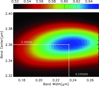
Figure 7. Contours produced by the optimisation algorithm exploring KISS survey SNR as a function of the bandwidth and centre wavelength of the chosen filter. The peak denoting an optimum filter for this case is marked.
The calculations optimising the SNR were found to yield a fairly robust outcome even under changing conditions (Figure 8). Increasing the thermal ambient environment acted, as would be expected, to shorten the red edge of the filter bandpass. The effect of varying target brightness was also explored, and found to have little effect on the optimisation except for cases of good ( ~ 1 arcsec) seeing. Then, only the filter bandwidth (not centre wavelength) was seen to increase by a modest ~ 10% as the flux of the target star was increased from 16th to 14th mag. Further simulations with the input blackbody varying from 2 000 to 10 000 K show that the star’s spectrum only slightly modifies the optimised filter curve. The optimised centre wavelength of the filter remains within 0.01 μm of nominal value of 2.375 μm and the bandwidth within 0.02 μm of nominal.
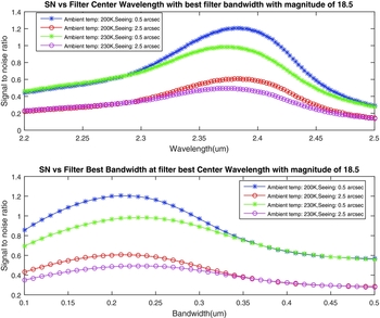
Figure 8. Filter SNR vs bandwidth and centre wavelength.
5.2. Influence of the sky background on the optimal bandpass
As illustrated in Figure 6, expectations for the red edge of the sky thermal background may be significantly pessimistic when applying data taken at the South Pole to expectations for the high plateau. As described above, we have formulated a simple model that might predict the shift of this emission edge with the expected colder and drier environment at Dome A. Over the assumed range of atmospheric conditions explored earlier, Table 1 gives the optimum filter properties for each model atmosphere. Moderate shifts at the 10% level towards the red are witnessed as expectations for the atmospheric background become colder and drier.
Table 1. Optimum filter properties (centre and bandpass in microns) as a function of atmospheric properties.
5.3. Effect of filter wings
The exponential rise in background in Figure 2 implies that we need to fully suppress a red leak from the K DARK filter wings. Simons & Tokunaga (Reference Simons and Tokunaga2002) note that the manufacturing specifications of their filters were designed so that out of band transmission < 0.0001 out to 5.6 μm and cut-on and cut-off wavelengths are to be attained within ± 0.5%. The KISS detector QE is specified to exceed 50% at 2.5 μm but falls to zero at approximately 3 μm. The filters of Simons & Tokunaga (Reference Simons and Tokunaga2002) have a roll-off spec: slope less than or equal to 2.5% where slope is defined to be: [ λ(80%)–λ(5%) ]/λ(5%). This is a steeper slope beyond 2.5 μm than the rise in Figure 2.
6 CONCLUSIONS
A realistic simulation of the performance of the instrumentation responsible for performing the KISS survey has been undertaken, exploring a range of possible environmental conditions and using the best currently available Antarctic site-testing data. The parameters of the bandpass filter to best exploit the previously reported K DARK window have been examined. These were found to vary only modestly over the range of likely assumptions for the environment and observing conditions, enabling a reasonably firm specification (λ0 2.375, Δλ 0.25 μm) to be made in furnishing the survey optical hardware.
ACKNOWLEDGEMENTS
We would like to thank all our colleagues on the KISS team for helpful discussions. The KISS camera is acquired through Australian Research Council LIEF grant LE15100024.


