


1 INTRODUCTION
Polarised radio emission arises generically from processes involving magnetised plasmas which are ubiquitous in the Universe. For example, polarisation appears, at some level, in all sources of synchrotron radiation. Measuring and studying the polarised emission (polarimetry) can provide insight into physical processes occurring in systems that range from our own atmosphere (the ionosphere), the intervening interstellar medium, and out to high-redshift galaxies. Science that depends on polarisation is part of the scientific motivation for a number of low-frequency instruments, however, doing accurate polarimetry at low frequencies is challenging.
Polarised sources generally depolarise with increasing wavelength as a result of Faraday depolarisation (Farnsworth, Rudnick, & Brown Reference Farnsworth, Rudnick and Brown2011; de Bruyn Reference de Bruyn2012; Gießübel et al. Reference Gießübel, Heald, Beck and Arshakian2013; Anderson et al. Reference Anderson, Gaensler, Feain and Franzen2015) during propagation from the radio source. Relevant regions include the extragalactic, galactic, interstellar, and interplanetary plasmas. When linearly polarised radiation propagates through a magnetised plasma, it undergoes Faraday rotation according to
 $$\begin{equation}
\chi (\lambda ^{2}) = \chi _{0} + \phi \lambda ^{2} = \chi _{0} + \int _{0}^{z} \text{d}z^{\prime }\ \text{RM}(z^{\prime })\ \lambda ^{2},
\end{equation}$$
$$\begin{equation}
\chi (\lambda ^{2}) = \chi _{0} + \phi \lambda ^{2} = \chi _{0} + \int _{0}^{z} \text{d}z^{\prime }\ \text{RM}(z^{\prime })\ \lambda ^{2},
\end{equation}$$
where χ(λ2) is the measured linear polarisation angle (rad) at wavelength λ (m), χ0 is the intrinsic polarisation angle (rad), ϕ is the Faraday depth (rad m−2), and the final term is the integral along the path from the source (z′ = 0) to the observer (z′ = z) of the rotation measure RM(z′), which depends on the spatially varying plasma density and component of the magnetic field along the path. Faraday rotation is particularly pronounced at long wavelengths because of the wavelength-squared dependence. The ionosphere introduces additional Faraday rotation which, if not corrected for, can further depolarise the signal. The fact that polarised signals are generally only a few percent as strong as the total intensity of the source itself means that measuring polarisation is challenging.
Polarimetry programmes are underway on a range of low-frequency instruments including the LOw-Frequency ARray (LOFAR, van Haarlem et al. Reference van Haarlem2013), the Long Wavelength Array (LWA, Ellingson et al. Reference Ellingson, Clarke, Cohen, Craig, Kassim, Pihlstrom, Rickard and Taylor2009), the Precision Array for Probing the Epoch of Reionization (PAPER, Parsons et al. Reference Parsons2010), and the Murchison Widefield Array (MWA, Tingay et al. Reference Tingay2013). In addition, the ongoing upgrade to the Giant Metrewave Radio Telescope (GMRT, Swarup Reference Swarup1990) will allow it to make sensitive polarimetric measurements. Processing polarimetric data pushes instruments to their software and hardware limits, since it is not only processor and data intensive, but also highly sensitive to instrumental and calibration errors. Hence, polarimetry is a powerful diagnostic tool when evaluating and characterising the performance of a new instrument (Sutinjo et al. Reference Sutinjo, O’Sullivan, Lenc, Wayth, Padhi, Hall and Tingay2015).
In this paper, we address some of the key technical challenges of doing polarimetry at low frequencies with the MWA. Section 2 outlines some of the early science results obtained with the MWA; Section 3 looks at software tools used to process MWA data; Section 4 summarises calibration methods that were developed for MWA processing; and Section 5 considers science that could be explored given our understanding of the MWA capabilities as it stands today and in the near future.
2 POLARIMETRY WITH THE MWA
The MWA is located at the Murchison Radio Observatory in Western Australia. It consists of an array of up to 128 connected tiles where each tile is comprised of a regular 4 × 4 grid of dual-polarisation dipoles. Tile beams are formed by combining the dipole signals in an analogue beamformer, using a set of switchable delay lines to provide coarse pointing capability (Tingay et al. Reference Tingay2013). The beamformer cannot provide continuous tracking, instead it uses a combination of discrete pointings and drift scans in what is referred to as ‘drift and shift’. The small size of each tile results in a field-of-view of ~600 deg2 at 150 MHz. In normal MWA operations, full polarisation correlation products (XX, YY, XY, YX) are stored by default. The work presented here uses the MWA array configuration present in the first 3 yrs of operations (Tingay et al. Reference Tingay2013).
The MWA observing bands are listed in Table 1. These bands are contiguous apart from a gap between 133.8 and 138.9 MHz to avoid interference from the ORBCOMM constellation of satellites that transmit in this frequency range (Offringa et al. Reference Offringa2015). While the MWA is capable of operating at frequencies above 230 MHz, RFI and the degraded response of the formed beam makes such observations problematic.
Table 1. Observing specifications for each MWA band assuming 40 kHz channel bandwidth. The lowest and highest observing frequency are specified by νmin and νmax, respectively. δϕ and |ϕmax| are the resolution and Faraday depth range available in each band. Where the maximum scale is smaller than δϕ, Faraday thick structures cannot be resolved. σν is the typical noise in Faraday depth cubes for a naturally weighted 2-min snapshot.
Studies of linear polarisation at low frequencies are complicated by the effects of Faraday rotation, as the degree of rotation is proportional to the wavelength squared. This can lead to bandwidth depolarisation if channel bandwidths are not small enough. However, with decreased channel bandwidth, sensitivity per channel is limited. Rotation measure (RM) synthesis (Brentjens & de Bruyn Reference Brentjens and de Bruyn2005) is typically adopted to determine the degree of Faraday rotation across the entire observed bandwidth. This takes advantage of the Fourier relationship between the complex polarised intensity as a function of wavelength squared and the Faraday dispersion function (FDF) F (ϕ) which is the polarised intensity as a function of Faraday depth (Burn Reference Burn1966).
The available resolution in Faraday space (δϕ) increases with the longest wavelength; the maximum range of Faraday depths that can be probed (|ϕmax|) is also dependent on the longest wavelength and the channel bandwidth (See Equations (61)–(63), Brentjens & de Bruyn Reference Brentjens and de Bruyn2005). Table 1 summarises these parameters for each MWA frequency band and also lists the maximum scale size. When the maximum scale is smaller than the resolution, it is not possible to resolve Faraday-thick structures. For the MWA, when using a single observing band, this is always the case. The channel width listed in Table 1 is 40 kHz; however, with the MWA correlator (Ord et al. Reference Ord2015), this can be reduced to as low as 10 kHz (in which case the listed maximum Faraday depth increases by a factor of four). In general, a 40 kHz channel width is adequate for most Galactic and extragalactic studies. However, finer channels may be warranted for studies of high-RM pulsars; e.g. observing PSR J0742−2822 with a RM of ~150 rad m−2 (Table 2) would require 20 kHz channel widths in the 89 MHz band to avoid bandwidth depolarisation.
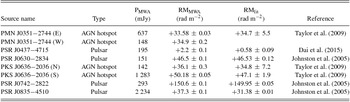
Table 2. Polarised point sources observed in the 216 MHz band in a GLEAM zenith drift scan (2013 November 25 14:44 to 19:53) and a −47° meridian drift scan (2013 Novemver 6 13:27 to 21:08). PMWA is the polarised flux density measured from MWA observations. RMMWA is the rotation measure determined from MWA observations (corrected for ionospheric Faraday rotation, see Section 4.3 for details). RMlit is the rotation measure in literature. The lowest frequencies used in the literature value RM measurements are 1 340 MHz (Taylor et al. Reference Taylor, Stil and Sunstrum2009), 700 MHz (Dai et al. Reference Dai2015), and 1 240 MHz (Johnston et al. Reference Johnston, Hobbs, Vigeland, Kramer, Weisberg and Lyne2005). The polarised eastern/western components for PMN J0351−2744 and northern/southern components for PKS J0636−2036 are listed separately.
The MWA has a compact and dense baseline configuration, with baselines as short as 7.7 m. The availability of short baselines for large-scale structure studies is shown in Figure 1; approximately, 15% (1 183) of the baselines are shorter than 120 m and provide sensitivity to structures a degree or more in extent. The MWA also provides baselines out to just under 3.0 km in extent, almost an order-of-magnitude improvement in resolution compared to the 32T prototype (Bernardi et al. Reference Bernardi2013), yet still within the regime where the effect of the ionosphere on each tile can be assumed to be the same (Lonsdale et al. Reference Lonsdale2009; Arora et al. Reference Arora2016).

Figure 1. The number of MWA baselines shorter than a given length (solid line) for a zenith pointing. The dotted grey line indicates the spatial scale that a given baseline is sensitive to.
The large number of baselines (8 128) provides excellent (u, v)-coverage for snapshot imaging. This allows short time-scale imaging without any significant degradation in image quality. This feature is particularly useful for calibration testing and primary beam characterisation.
2.1. Compact source polarimetry
An early concern regarding polarimetry with the MWA was that beam depolarisation would effectively depolarise all intrinsically linearly polarised signals. Beam depolarisation occurs when there are spatial fluctuations in polarisation angle across the synthesised beam (which is of order 2 arcmin–5 arcmin with the MWA), resulting in a reduction in the measured linear polarisation. The 32-tile MWA prototype (32T) provided the first hints of what may be achievable with the full MWA. With baselines extending out to ~350 m, 32T provided limited (u, v)-coverage out to ~4° scales and a resolution of ~16 arcmin at 189 MHz. Despite this, 32T was able to detect a linearly polarised extragalactic source (PMN J0351−2744) and large-scale linearly polarised diffuse emission (Bernardi et al. Reference Bernardi2013).
Observations from the MWA show PMN J0351−2744 is clearly resolved into a double linearly polarised source. The resolution of ~2 arcmin at 216 MHz shows that the polarised component was associated with the edge of the source seen in total intensity (Figure 2). This shows that the scale size of the emitting regions in total intensity is generally greater than that for linear polarisation, so that the intrinsic fractional polarisation of the latter will be underestimated in observations with low spatial resolution. Figure 3 shows the FDF for the eastern hotspot. The measured RM of +33.6 rad m−2 for the hotspot is consistent with the RM determined by Bernardi et al. (Reference Bernardi2013).
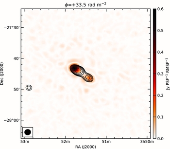
Figure 2. Polarised intensity map of the source PMN J0351−2744 taken at a Faraday depth of ϕ = +33.5 rad m−2 (corrected for ionspheric Faraday rotation, see Section 4.3 for details). Contours show total intensity with the lowest contour at 1.45 Jy PSF−1 and subsequent contours increasing by a factor of
 $\sqrt{2}$
. The synthesised beam size is 2 arcmin × 1.8 arcmin FWHM at a position angle of −83°.
$\sqrt{2}$
. The synthesised beam size is 2 arcmin × 1.8 arcmin FWHM at a position angle of −83°.

Figure 3. Faraday dispersion function for the eastern hotspot of the polarised source PMN J0351−2744 at 216 MHz. The eastern hotspot peaks at a Faraday depth of +33.6 rad m−2 and a flux density of 630 mJy PSF−1 RMSF−1.
We conducted a search for linearly polarised point sources using data taken as part of the GLEAM survey (Wayth et al. Reference Wayth2015; Hurley-Walker et al. Reference Hurley-Walker2017). We limited the search to regions covered by the MWA Commissioning Survey (Hurley-Walker et al. Reference Hurley-Walker2014) as the catalogue from this survey provided an excellent low-frequency sky model for calibration purposes. RM synthesis and a conservative 10-sigma threshold was used to identify linearly polarised sources in the RM cube for each 2-min snapshot. The search was shallow and only used data from the 216 MHz band (to minimise frequency-dependent depolarisation effects), but it provided the first data to study the polarimetric characteristics of the instrument. First, the beam model could be verified as sources transit through the beam. Second, polarised source candidates could be validated if they appeared in neighbouring 2-min snapshots and with a similar RM and position. Third, the flux, position, and RM stability could be tracked for confirmed polarised sources. Finally, deeper images could then be made by integrating multiple snapshots in time.
We also made targeted measurements for 4 348 known polarised sources listed in Taylor, Stil, & Sunstrum (Reference Taylor, Stil and Sunstrum2009) and 72 known pulsars in Manchester et al. (Reference Manchester, Hobbs, Teoh and Hobbs2005). In total, six sources were detected in a 6 000 deg2 region, four were found in the −27° drift scan and two in the −47° drift scan. The sources and their polarisation parameters are summarised in Table 2.
Four of the six sources detected are pulsars and are the four brightest known pulsars listed in the ATNF Pulsar CatalogueFootnote 1 v1.54 (Manchester et al. Reference Manchester, Hobbs, Teoh and Hobbs2005) in the 6 000 deg2 region surveyed (a source density of one per 1 500 deg2, see Section 5.1 for further discussion). Pulsars are easier to detect in polarisation compared to other polarised sources at MWA wavelengths because (a) they generally have high fractional polarisation (so are easier to separate from polarisation leakage); and (b) they have negligible angular extent (and so do not suffer from depolarisation). This may make polarisation searches an interesting technique for discovering pulsars in imaging surveys; see Section 5.3.
All of the RMs measured for the polarised sources are consistent with RM values found in literature (with an additional ±2 rad m−2 margin of error where ionospheric corrections were not made in the literature) apart from PSR J0835−4510. This is the Vela pulsar and has an RM that varies on a time-scale of about a year as a result of being embedded in an ionised cloud formed by a pulsar wind nebula and the Vela supernova remnant (Hamilton et al. Reference Hamilton, McCulloch, Manchester, Ables and Komesaroff1977; Hamilton, Hall, & Costa Reference Hamilton, Hall and Costa1985; Johnston et al. Reference Johnston, Hobbs, Vigeland, Kramer, Weisberg and Lyne2005).
PKS J0636−2036 is the brightest linearly polarised extragalactic source detected with the MWA to date. It is also the only extragalactic source that has been detected in all five of the MWA frequency bands. As a result, it has become the default source for testing polarimetric behaviour of the MWA.
2.2. Circular polarisation
A majority of astronomical sources do not emit significant circular polarisation. As a result, images of circular polarisation (Stokes V) are not limited by source confusion or sidelobe confusion and can achieve sensitivity levels that approach thermal noise. This also means that the angular resolution of the instrument is not critical for detection and is only required to improve the localisation of the source.
Circular polarisation is not affected by Faraday rotation and can be processed in a similar manner to Stokes I imaging by treating the entire frequency band in a continuum-like mode (assuming the sign of circular polarisation does not change across the band). However, as many sources which emit in Stokes V are particularly energetic and may exhibit flaring or transient behaviour, care must be taken in choosing the time-scale over which integration is performed when searching for variable circular polarisation. If the event is brief but integrated over an extended period of time, then the signal associated with the event will be diluted. Similarly, if the sign of polarisation flips over the course of the integration (e.g. Lynch et al. Reference Lynch, Murphy, Kaplan, Ireland and Bell2017a, Reference Lynch, Lenc, Kaplan, Murphy and Anderson2017b), then this can reduce the signal.
The first sources detected in circular polarisation with the MWA were pulsars. For example, PSR J0835−4510 exhibits circular polarisation across all five MWA frequency bands and PSR J0437−4715 is also clearly detected in Stokes V images. Lenc et al. (Reference Lenc2016) demonstrated that long integrations in Stokes V could be used to detect weak pulsars in deep fields. This technique could be used to detect pulsars and other circularly polarised sources such as flare stars (Lynch et al. Reference Lynch, Lenc, Kaplan, Murphy and Anderson2017b) and potentially extrasolar planets (Murphy et al. Reference Murphy2015).
2.3. Diffuse polarisation
Low-frequency observations of diffuse polarisation are sensitive to small changes in Faraday rotation as a result of fluctuations in the magnetised plasma, which are difficult to detect with observations at high frequencies. Early low-frequency observations with synthesis telescopes, e.g. WSRT between 325 and 375 MHz (Wieringa et al. Reference Wieringa, de Bruyn, Jansen, Brouw and Katgert1993; Haverkorn, Katgert, & de Bruyn Reference Haverkorn, Katgert and de Bruyn2000, Reference Haverkorn, Katgert and de Bruyn2003a, Reference Haverkorn, Katgert and de Bruyn2003b, Reference Haverkorn, Katgert and de Bruyn2003c) and WSRT at 150 MHz (Bernardi et al. Reference Bernardi2009, Reference Bernardi2010) were only sensitive to structures smaller than ~1°. The structures detected were weak and would require significant integration time to detect with the MWA.
More recent observations with LOFAR at 150 MHz (Iacobelli, Haverkorn, & Katgert Reference Iacobelli, Haverkorn and Katgert2013; Jelić et al. Reference Jelić2015; Van Eck et al. Reference Van Eck2017) achieved sensitivity to spatial scales up to ~5° by utilising a high-band antenna dual-inner mode (van Haarlem et al. Reference van Haarlem2013). While these observations also provided baselines significantly longer than currently available with the MWA, enabling a study of weak diffuse structures at a resolution hardly affected by beam depolarisation (Jelić et al. Reference Jelić2015), they provided relatively few short baselines and so sensitivity to large-scale structures was limited. Single dish polarimetric observations at long wavelengths provide access to large-scale structure, e.g. Mathewson & Milne (Reference Mathewson and Milne1965), but single dish observations below 300 MHz lack resolution and sensitivity.
Observations at 189 MHz with the MWA 32T (Bernardi et al. Reference Bernardi2013) provided the first indication of what the MWA may be able to detect. Its relatively compact baselines provided limited sensitivity out to ~4° scales, which was enough to demonstrate that linearly polarised diffuse emission from the local interstellar medium could be detected with an MWA-like array.
When the MWA was used to observe diffuse linear polarisation, a surprising outcome was that the emission was bright and present on larger scales than previously observed (Lenc et al. Reference Lenc2016). Figure 4 shows an example of the diffuse emission observed at 216 MHz with the MWA; the image was formed by combining 24 × 2 min snapshots from a zenith drift scan. The polarised emission is so dominant that it is easily detected in 2-min snapshot images with a signal-to-noise of ~70.

Figure 4. Polarised intensity observed over a zenith drift scan (not corrected for ionospheric Faraday rotation) in the 216 MHz band. The flux scale is in Jy PSF−1. The synthesised beam, shown as a filled ellipse, is 54 arcmin×47 arcmin FWHM at a position angle of −1.8°.
The high signal-to-noise at which the MWA detects this diffuse polarised structure provides a valuable resource. For example, XY-phase calibration ideally requires the presence of a bright polarised source (see Section 4.2). Similarly, the emission can be used to monitor the polarimetric response across the beam and can provide a reference against which temporal changes in Faraday rotation can be monitored.
3 PROCESSING FOR POLARIMETRY
Most radio data reduction packages were not designed with fixed dipole-based instruments in mind. As such, they have built in assumptions that are generally only valid for targeted, dish-based instruments. Nonetheless, packages such as Miriad (Sault, Teuben, & Wright Reference Sault, Teuben, Wright, Shaw, Payne and Hayes1995) and casa (McMullin et al. Reference McMullin, Waters, Schiebel, Young, Golap, Shaw, Hill and Bell2007) were used in early MWA processing pipelines (Hurley-Walker et al. Reference Hurley-Walker2014) and are suitable for basic calibration and imaging in Stokes I.
However, these packages are unable to solve for full wide-field polarimetric effects and so their use for polarimetry is restricted to narrow-field imaging of Stokes Q at zenith. Generating the full spectral cubes required for polarimetry is computationally expensive as these packages were not designed to work within modern high-performance computing (HPC) environments.
Recent processing pipelines for the MWA use packages that are designed to work in HPC environments and the specific calibration and imaging needs of fixed dipole-based instruments. The three packages in use for polarimetry are the Real-time system (rts, Mitchell et al. Reference Mitchell, Greenhill, Wayth, Sault, Lonsdale, Cappallo, Morales and Ord2008; Ord et al. Reference Ord2010); mitchcal (Offringa et al. Reference Offringa2016) together with wsclean Footnote 2 (Offringa et al. Reference Offringa2014); and Fast Holographic DeconvolutionFootnote 3 (fhd, Sullivan et al. Reference Sullivan2012). These packages are described in further detail in the following sections. Note that the rts package was used for all processing described in this paper.
It is worth briefly mentioning the typical visibility weighting schemes used for MWA polarimetry. For polarimetry of diffuse polarisation, natural weighting works well with the dense baseline distribution in the MWA core. This can be further optimised by removing baselines outside of the MWA core as it results in a more Gaussian synthesised beam (see Lenc et al. Reference Lenc2016). For compact source polarimetry, robust weighting (with robustness of −1) works well. Further improvement is obtained by removing the shortest baselines from the MWA core to avoid excessive down-weighting of the longest baselines.
3.1. Real-time system
The rts is the only one of these packages that can take advantage of Graphics Processing Units (GPUs) to increase performance (it can also run on CPUs if GPUs are unavailable). The rts calibrates based on a local sky model and can generate full spectral resolution Stokes cubes that are corrected for dipole projection effects and wide-field effects across the entire field-of-view. These can be produced in real time for small fields-of-view with limited peeling or near real time for larger fields.
Prior to imaging, the rts can optionally peel out sources in a local sky model from visibility data to reduce (PSF) sidelobe confusion. It also solves for ionospheric positional shifts and flux density variations during the peeling process.
One drawback of the rts is that it cannot perform deconvolution. This is not critical for polarimetry but it can help to reduce PSF sidelobes of particularly bright Stokes I sources that leak signal into the polarisation products. If deconvolution is necessary, the rts can export calibrated and peeled visibilities in FITS format and these can be deconvolved outside of the package (preferably with an algorithm that deals appropriately with the complex nature of polarisation, see Pratley & Johnston-Hollitt Reference Pratley and Johnston-Hollitt2016). Another constraint is that the imaging field-of-view in GPU mode is limited by GPU memory constraints (this is less of an issue in CPU mode).
3.2. MitchCal and wsclean
MitchCal (Offringa et al. Reference Offringa2016) is a custom implementation of the direction-independent full-polarisation self-calibration algorithm used by the rts (Mitchell et al. Reference Mitchell, Greenhill, Wayth, Sault, Lonsdale, Cappallo, Morales and Ord2008). In combination with wsclean, this set of tools can generate full Stokes images. The tools have mostly been used to generate and deconvolve continuum maps but can be adapted to generate spectral cubes.
As with the rts, this set of tools provides a means to calibrate for ionospheric shifts. It also provides direction-dependent calibration by clustering sources to improve calibration signal-to-noise in the direction of the cluster. A further advantage, in comparison to the rts, is the ability to perform efficient wide-field deconvolution.
3.3. FHD
fhd (Sullivan et al. Reference Sullivan2012) is an imaging and calibration algorithm designed for wide field-of-view interferometers with direction- and antenna-dependent beam patterns. It has been used for EoR science (Jacobs et al. Reference Jacobs2016), but it includes functionality for calibration, imaging, deconvolution, and simulation that can be applied more generally.
Using a widefield polarised antenna beam model, FHD calibrates the X and Y dipoles separately to match an input sky model (typically 104 sources). The global phase between the X and Y dipoles is fit by minimising the apparent V power, explicitly assuming there is very little real V power on the sky and little of the Q polarisation is mixed to V in a crossed dipole array. If given a sky model with polarised emission, FHD can fit a global ionospheric Faraday mixing angle between Q and U. This mixing angle is used to correct for ionospheric rotation when making the diffuse image cubes.
Deconvolution in full Stokes I, Q, U, and V is possible with FHD. This can be used to generate models in other Stokes parameters besides I, and may be essential to making diffuse maps without bright Stokes I leakage. FHD also has the ability to generate a separate beam model for each antenna to help reduce leakage if that level of detail is known.
4 MWA POLARISATION CALIBRATION
There are three aspects of MWA calibration that are particularly relevant to polarimetry: calibrating for the primary beam shape, calibrating for XY-phase and correcting for ionospheric Faraday rotation. We now discuss each aspect in turn.
4.1. Beam model
Early analysis of MWA drift scan images revealed that many sources appeared to have significant levels of linear and circular polarisation towards the edge of the primary beam. This effect is often referred to as ‘leakage’, where emission from Stokes I appears to leak into the other Stokes parameters. For drift scans passing through zenith (−27°) and observed in the 154 MHz band, the level of leakage was consistent with that measured by Bernardi et al. (Reference Bernardi2013); typically of the order of ~1% in the beam centre and ~4% towards the edge of the field.
However, for beamformer pointings away from zenith and for observations in the highest frequency bands, the measured leakage was higher. For example, the plot on the left in Figure 5 shows the measured percentage leakage in Stokes Q, U, and V measured in the MWA 216-MHz band for field sources as a function of declination for a −13° declination meridian scan. In this plot, the leakage in Q increases from 12% near zenith to nearly 40% at 0° declination. While leakage in U and V also show declination dependent trends, they occur at much lower levels and are not as problematic.

Figure 5. Left: Declination-dependent leakage observed in the MWA 216 MHz band for a δ = −13° declination meridian scan using an analytic beam model to correct for instrumental polarisation. The plot shows the median fractional polarisation for Stokes Q, U, and V where q = Q/I, u = U/I and v = V/I. The fractional linearly polarised intensity p is also shown where
 $p=\sqrt{\text{Q}^{2}+\text{U}^{2}}/\text{I}$
. Right: Same as left but using the Sutinjo et al. (Reference Sutinjo, O’Sullivan, Lenc, Wayth, Padhi, Hall and Tingay2015) beam model.
$p=\sqrt{\text{Q}^{2}+\text{U}^{2}}/\text{I}$
. Right: Same as left but using the Sutinjo et al. (Reference Sutinjo, O’Sullivan, Lenc, Wayth, Padhi, Hall and Tingay2015) beam model.
These observed trends are symptomatic of errors in the primary beam model. Stokes Q is generally affected the most as it is formed from the same instrumental polarisations as Stokes I, i.e. I
 $=\frac{1}{2}($
XX+YY) and Q
$=\frac{1}{2}($
XX+YY) and Q
 $=\frac{1}{2}($
XX−YY), and so these contain the bulk of the total intensity signal. Stokes U and V are formed from the cross polarisations (XY and YX) which do not have significant signal content. As such, any errors in correcting for the XX and YY for the beam shape using a primary beam model result in some portion of a large signal leaking into Stokes Q. Primary beam model errors can also result in a scaling error in Stokes I, as noted by Hurley-Walker et al. (Reference Hurley-Walker2014) and Hurley-Walker et al. (Reference Hurley-Walker2017). This error manifested itself as a declination and frequency-dependent scaling error in Stokes I.
$=\frac{1}{2}($
XX−YY), and so these contain the bulk of the total intensity signal. Stokes U and V are formed from the cross polarisations (XY and YX) which do not have significant signal content. As such, any errors in correcting for the XX and YY for the beam shape using a primary beam model result in some portion of a large signal leaking into Stokes Q. Primary beam model errors can also result in a scaling error in Stokes I, as noted by Hurley-Walker et al. (Reference Hurley-Walker2014) and Hurley-Walker et al. (Reference Hurley-Walker2017). This error manifested itself as a declination and frequency-dependent scaling error in Stokes I.
Early imaging efforts with the MWA used an analytic beam model of a simple short dipole with an ideal array factor derived by Bowman et al. (Reference Bowman2007). This relatively simple model was a good approximation of an MWA tile at an optimal observing frequency of 154 MHz and towards the zenith. However, the model diverges from observations at higher frequencies bands where the simple short-dipole model no longer holds. Two approaches were taken in an attempt to reduce such errors: improvements in the beam model and mitigation techniques using empirical data. These are described in detail in the following sections.
4.1.1. Beam improvements
To improve the beam model, Sutinjo et al. (Reference Sutinjo, O’Sullivan, Lenc, Wayth, Padhi, Hall and Tingay2015) performed simulations that incorporated both mutual coupling and embedded element patterns. Initial testing of an implementation of this model shows an improvement in overall polarisation leakage. The plot on the right in Figure 5 shows the improvement obtained in comparison to the analytic beam model. Leakage from Stokes I to Stokes Q shows a dramatic reduction in the new beam model, however, there is an associated increase in leakage measured in Stokes U and V.
Despite the slight increase in leakage in Stokes U and V, the overall factor of 3−4 reduction in polarisation leakage in this beamformer pointing and frequency band is a significant improvement. It should be noted that this a worst-case scenario as it highlights one of the most severely affected bands and beamformer pointings; furthermore, no attempt was made to limit the leakage with in-beam self-calibration. Further testing is currently being performed on the improved beam model to compare its performance against the analytic beam for various beamformer pointings and observing bands (Sokolowski et al. Reference Sokolowski2017).
4.1.2. Mitigating leakage in polarisation
Despite the improvements in primary beam models, there will always be some errors due to imperfections in the models and in the MWA dipoles themselves. Differences in orientation, environment, and the number of dipole failures within a tile affect the true beam response of the tile. The more complex the beam model becomes, the more computationally intensive it is to calculate during the calibration and imaging process.
For small fields-of-view around a bright source, in-beam calibration with a sky model can reduce beam-related leakage effects close to the dominant source of the sky model by assuming it is unpolarised. In general, this is a reasonable assumption given that few sources are polarised at long wavelengths and those that are typically have a fractional polarisation of a few percent. However, this only reduces leakage in the vicinity of the dominant source. Further away from the dominant source, polarisation leakage once again becomes evident.
An alternative to in-beam calibration is measuring and removing the beam-related errors empirically. The field-of-view and (u, v)-coverage of the MWA means that the beam can be mapped with short (2-min) snapshots over the course of an extended drift scan. This approach was taken by Hurley-Walker et al. (Reference Hurley-Walker2017) and Callingham (Reference Callingham2017) to correct for declination and frequency-dependent flux-scale errors observed in Stokes I for point sources as they drifted through the MWA beam. These corrections also highlighted spatial calibration discrepancies in other long wavelength surveys (Hurley-Walker Reference Hurley-Walker2017).
A similar approach can be applied to Stokes Q, U, and V by mapping the observed leakage of point sources as they drift through a given beamformer pointing. By assuming sources are unpolarised, the leakage can be modelled spatially across the beam. Figure 6 shows the measured leakage in field sources for one beamformer pointing in observations of the flare star UV Ceti.

Figure 6. A sample demonstrating the fitting of point-source leakage over the observed field-of-view. The points were taken from one of the beamformer pointings used during a ‘drift and shift’ observation. Fits were performed separately for different beamformer pointings and for each of the different Stokes parameters (Q, U, and V). The X and Y axis are in units of pixels for a 25° × 25° field.
A spatial fit of the leakage can be determined for each Stokes parameter and for each beamformer pointing. The fit is then used to scale and subtract the Stokes I images from each of the Stokes Q, U, and V images, removing the leaked component of Stokes I. Figure 7 demonstrates the dramatic improvement that results from this method and the subsequent detection of a linearly polarised flare in UV Ceti (Lynch et al. Reference Lynch, Murphy, Kaplan, Ireland and Bell2017a). Prior to subtraction, the field was dominated by polarisation leakage but after subtraction only a single source, UV Ceti, dominated the field with 10σ significance.

Figure 7. The polarised intensity map for the UV Ceti field before leakage subtraction in Stokes Q and Stokes U (left), and after leakage subtraction (right). In the leakage-subtracted image, the dominant source in the field (highlighted with a red circle) is UV Ceti shown during a flare.
4.2. X–Y phase calibration
When calibration of linearly polarised antennas is performed on an unpolarised source, the phase relationship between the orthogonal X and Y polarisations cannot be solved for. Any residual phase results in leakage from linear polarisation into circular polarisation (Stokes V). To solve for the X–Y phase, calibration against a polarised source is required (Sault, Hamaker, & Bregman Reference Sault, Hamaker and Bregman1996).
Traditionally, X–Y phase is calibrated against a known polarisation point-source calibrator. The challenge is that compact linearly polarised sources suitable for calibration (Bernardi et al. Reference Bernardi2013) are rare at long wavelengths (see Section 2.1).
An alternative is to use diffuse polarised emission. As shown in Section 2.3, the dense MWA core provides excellent sensitivity to large-scale structure. The diffuse polarised structure from the ISM has sufficient signal-to-noise to enable the X–Y phase to be solved for.
Figure 8 shows the Stokes U and Stokes V images from observations at 154 MHz (Lenc et al. Reference Lenc2016). No circular polarisation is expected in diffuse emission from the local ISM, yet there are clear diffuse structures in the Stokes V map. These structures closely resemble those that appear in Stokes U but at about the 20–30% level.

Figure 8. The top two figures show the similarity between Stokes U (left) and Stokes V (right) in MWA observations of the EoR-0 field at 154 MHz. This demonstrates the effect of leakage from Stokes U into Stokes V caused by uncorrected X–Y phase. The bottom two figures show Stokes I (left) and Stokes V (right) after applying a correction for the X–Y phase shown in Figure 9. The remaining features in Stokes V are dominated by leakage from Stokes I. This leakage is associated with errors in the beam model, see Section 4.1. Note the different flux density scales in the different images.
Diffuse linear polarisation is evident across the southern sky, as shown in Figure 4. The ubiquity and strength of this signal makes it an ideal alternative for use in X–Y phase calibration. The emission appears with sufficient signal-to-noise to allow the X–Y phase to be measured as a function of frequency, see Figure 9, demonstrating that the phase is independent of frequency.

Figure 9. X–Y phase measured as a function of frequency using diffuse polarised emission from the EoR-0 field.
Applying a correction for the X–Y phase derived from the observed features in Stokes U and Stokes V results in a 5–10% improvement in Stokes U and a 20–30% improvement in Stokes V. After the correction for X–Y phase, the corrected Stokes V image (Figure 8) is now dominated by leakage from Stokes I at the ~1% level. This residual leakage results from errors in the beam model, as described in Section 4.1.
4.3. Ionospheric Faraday rotation
Long-wavelength polarimetry allows us to measure Faraday rotation with high precision. So much so, that Faraday rotation introduced by the ionosphere is the dominant source of error in the observed RM. In typical MWA nighttime observations at high elevations, this effect is small. However, applications that require high-accuracy measurements of source RM still need to correct for the ionospheric component. Similarly, to avoid depolarisation, observations require calibration for ionospheric Faraday rotation when integrating over time periods throughout which the ionospheric conditions vary significantly. The time period over which this can be critical can be on the order of an hour in the lowest MWA band (over which the Faraday rotation can vary on the order of ~0.3 rad m−2 at zenith during calm ionospheric conditions at night). The highest MWA band is more resilient to ionospheric effects, but corrections must still be considered if integrating data from separate days in which the ionospheric conditions varied significantly (such variations can typically be of order several rad m−2).
4.3.1. Ionospheric modelling
A number of tools are available to estimate ionospheric content and ionospheric Faraday rotation using Global Positioning System observations and models of the Earth’s magnetic field. Examples of these include ionFR (Sotomayor-Beltran et al. Reference Sotomayor-Beltran2013), RMextract Footnote 4 , and albus (Willis et al. Reference Willis, Mevius, Anderson, O'Sullivan, Lenc, Arora, Gaensler and Landecker2017). While these tools struggle to predict fine spatial and temporal detail in the ionosphere, they provide sufficient resolution to correct for the mean electron content of the ionosphere.
Figure 10 demonstrates the improvement gained by applying a correction for ionospheric Faraday rotation. The plot shows the uncorrected and corrected RM measured for polarised emission seen in the southern hotspot of PKS J0636−2036 as a function of time, as observed in the lowest MWA frequency band. Prior to correction, the overall RMS in RM over the duration of the observing period is 0.085 rad m−2. As can be seen in Figure 11, this is sufficient to completely depolarise the signal of this otherwise bright source. However, when the RM is corrected for ionospheric effects, the RMS in RM reduces to 0.03 rad m−2 and the source emission is recovered. In addition, the ionospheric correction has enabled the detection of a weaker northern component of this source. After correction, the measured RMS in RM is approximately three times higher than the expected RMS (0.01 rad m−2), most likely as a result of the coarse resolution of the ionospheric modelling in both time and sky position.

Figure 10. Variation in observed rotation measure in the southern hotspot of PKS J0636−2036 as a function of time in the lowest MWA band (89 MHz). Blue points show the measured RM before ionospheric calibration and the Black points show the measured RM after ionospheric calibration. The red line shows the mean value of RM in each instance.
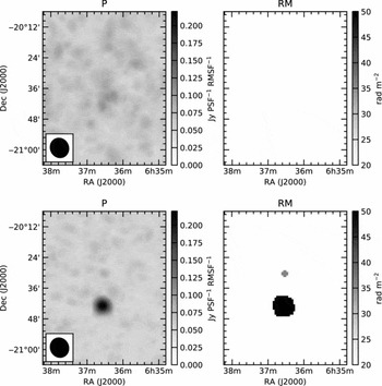
Figure 11. Polarised intensity (left) and rotation measure (right) maps for PKS J0636−2036 in the lowest MWA band (89 MHz) uncorrected (top) and corrected (bottom) for ionosphere Faraday rotation. The rotation measure maps are masked to show only peaks with 6σ significance (for a measured noise of 1σ = 13 mJy PSF−1 in polarised intensity).
4.3.2. Ionospheric self-calibration
The example shown in Figure 10 assumed that we had no a priori information regarding the RM of the source. If there is a sufficiently bright polarised source in the field-of-view and the source has a predetermined RM or we can assume that it has a constant RM, then there is no need to do ionospheric modelling. Instead, Stokes Q and U can be rotated on a per-snapshot basis to ensure that the measured RM of the source remains constant. In this sense, it is possible to self-calibrate against ionospheric Faraday rotation.
One benefit of this method is that GPS data is often not available until weeks after the event. A second benefit is that ionospheric modelling does not always give accurate estimates for ionospheric Faraday rotation at the source location and observation time. Ionospheric self-calibration provides accurate RM information without the need for external information, after initially correcting for the ionosphere using a model and the RM of the source is known.
The main limitation of ionospheric self-calibration is that it requires a sufficiently bright polarised source in the observed field-of-view. However, as discussed in Section 4.2, diffuse polarisation provides an alternate source of polarisation against which calibration can be performed. Lenc et al. (Reference Lenc2016) demonstrated that this diffuse polarised emission could not only be used to track the effects of ionospheric Faraday rotation as a function of time (on 2-min time-scales) but also spatially over the entire MWA fieldof-view.
4.3.3. Mapping the ionosphere
The use of diffuse polarisation to perform self-calibration for ionospheric Faraday rotation presents an interesting possibility. Assuming that a Galactic RM map can be determined, which is also one of the goals of the SKA higher frequency RM Grid experiment (e.g. Johnston-Hollitt et al. Reference Johnston-Hollitt2015, and references therein), this map can be used as a template against which the ionospheric contribution can be mapped. Such a map could be used to determine the total-electron content (TEC) between the observer and the diffuse Galactic ISM, given a model for the geomagnetic field. This complements existing ionospheric mapping capabilities demonstrated with the MWA that measured spatial gradients in TEC (Loi et al. Reference Loi2015a, Reference Loi2015b, Reference Loi2015c) as opposed to absolute TEC. It would also enable wide-field studies of the ionosphere over finer temporal and spatial scales than is currently possible with ionospheric modelling tools.
4.3.4. Validating polarisation with the ionosphere
A side effect of polarisation leakage is that it manifests itself as a peak at RM ≈ 0 rad m−2; an effect observed in wide-field polarimetric observations with parabolic dishes at shorter wavelengths, e.g. Jagannathan et al. (Reference Jagannathan, Bhatnagar, Rau and Taylor2017). This can complicate the detection of real polarised sources with low RM. However, Lenc et al. (Reference Lenc2016) showed that the ionosphere can be used as a tool to detect such sources. Using multiple observations of the source over multiple epochs where the ionospheric conditions vary significantly can aid to push the measured RM of the source away from an RM of 0 rad m−2 allowing a separation of the source RM from the peaks caused by polarisation leakage.
Ionospheric Faraday rotation can also be used to validate polarised source candidates. By cross-correlating the FDFs of a source over multiple epochs, if the observed shift in source RM matches the shift expected by the ionosphere, then this provides greater confidence that the candidate source is real.
4.4. Remaining calibration challenges
The regular spacing of dipoles in a MWA tile results in a primary beam with significant primary beam grating lobes. Bright sources located in these gratings generate PSF sidelobe structures that sweep through the main beam as a function of frequency and time. These sidelobe structures can appear highly polarised if they originate from low elevations where the beam has a different polarised response, and deconvolution will be limited because the polarised response for such sources is not well modelled. This can result in false detections in Faraday space and limit the detection of weakly polarised sources.
For bright point sources, ‘peeling’ can be used to minimise the PSF sidelobe structure from a problematic source (Mitchell et al. Reference Mitchell, Greenhill, Wayth, Sault, Lonsdale, Cappallo, Morales and Ord2008). Peeling refers to the (u, v)-plane subtraction of the source model multiplied by its best fit Jones matrices so as to remove the source contribution from all four instrumental polarisations. For unresolved sources, this is difficult to achieve because a well-defined model is required. Furthermore, at low elevation, the projected baselines of the MWA are severely foreshortened making the array sensitive to extended sources (Thyagarajan et al. Reference Thyagarajan2015). In particular, the presence of the Galactic plane in one of the primary beam grating lobes can be detrimental for imaging. The methods for dealing with such cases are limited, typically requiring avoiding beamformer pointings where such instances occur. Alternatively, an adaptation of SAGECal for use with MWA observations may be used to remove PSF sidelobe structures using direction dependent calibration (Yatawatta et al. Reference Yatawatta, Zaroubi, de Bruyn, Koopmans and Noordam2008; Kazemi et al. Reference Kazemi, Yatawatta, Zaroubi, Lampropoulos, de Bruyn, Koopmans and Noordam2011). Further investigation is required to solve this problem.
Another remaining challenge is calibrating for the absolute polarisation angle. Currently, the polarisation angle is left unconstrained during the calibration procedure. This is reasonable for polarimetry over a single observing session but may lead to depolarisation when integrating over multiple observing sessions if the polarisation angle is inconsistent in each session. In practice, absolute polarisation angle calibration is complicated by beamformer pointing changes and ionospheric Faraday rotation and the solution to this problem requires further development. Especially when there are little or no reference measurements at low frequencies, and an artificial cal signal cannot be injected into the receivers, as in single dish observations, e.g. Johnston et al. (Reference Johnston, Hobbs, Vigeland, Kramer, Weisberg and Lyne2005).
5 FUTURE DIRECTIONS FOR POLARIMETRIC SCIENCE
Our experience with MWA has laid the foundations for future work in the study of polarimetric science. In this section, we discuss some of the outstanding questions that polarimetric observations can give us insight into.
5.1. Low-frequency polarisation source counts
Linear polarisation source counts are well studied at 1.4 GHz (e.g. Taylor et al. Reference Taylor2007; Hales et al. Reference Hales, Norris, Gaensler and Middelberg2014; Rudnick & Owen Reference Rudnick and Owen2014) and at 20 GHz (Massardi et al. Reference Massardi2013). However, at low frequencies, there have been only a small number of detections to date. Two surveys with the MWA detected only two extragalactic sources brighter than 300 mJy PSF−1 (in Section 2.1, a shallow survey over ~6 000 deg2) and four 30–300 mJy PSF−1 in a deeper survey over ~400 deg2 (Lenc et al. Reference Lenc2016). A pointed observation with LOFAR, with a resolution of 20 arcsec, detected one source every ~2 deg2 for sources between 0.5 and 6.0 mJy PSF−1 in a ~17 deg2 region (Mulcahy et al. Reference Mulcahy2014). Jelić et al. (Reference Jelić2015) also detected 15 polarised sources within a ~25 deg2 region towards 3C196; however, the details (location, flux density, polarisation fraction, and RM) of the sources were not presented.
MWA observations can provide an improved understanding of the polarised source population above ~10 mJy PSF−1 over the entire sky because of the wide-field capabilities of the instrument. If the findings of Lenc et al. (Reference Lenc2016) hold true over the entire sky, then of order ~250 polarised extragalactic sources should be detected. At this level, sources counts will become more statistically relevant.
As described in Section 2.1, a significant factor that limits the effectiveness of point-source polarimetry with the MWA is its limited angular resolution. The 2 arcmin–4 arcmin synthesised beam of the MWA results in significant beam depolarisation in all but the simplest of sources. This may improve in future as the MWA project considers extended baseline lengths. Such an extension will have a two-fold improvement as it will not only reduce beam depolarisation effects but also improve sensitivity in imaging modes that use uniform weighting as the longest baselines will no longer be significantly down-weighted.
5.2. Low-frequency depolarisation of radio galaxies
Low-frequency linear polarisation observations of extragalactic radio sources can enable detailed studies of magnetised plasma along the entire line of sight from the emitting source to the telescope. The very large wavelength-squared coverage of low-frequency telescopes means they can outperform traditional centimetre radio facilities by more than two orders of magnitude in terms of the RM resolution (<1 rad m−2) of the observations (Table 1). However, finding brightly polarised extragalactic sources at low frequencies has been challenging due to the often poor angular resolution and the strong effect of Faraday depolarisation (e.g. Farnsworth et al. Reference Farnsworth, Rudnick and Brown2011). Therefore, obtaining a better understanding of exactly how radio galaxies depolarise at low frequencies is important for designing experiments to detect a sufficiently large sample that would allow statistical studies of the emitting sources themselves as well as the foreground magnetoionic material (e.g. Gaensler et al. Reference Gaensler2015; Vacca et al. Reference Vacca2015).
There are multiple models describing the depolarisation behaviour of extragalactic sources as a function of wavelength. The predictions made by these models tend to diverge at long wavelengths, e.g. an exponential fall-off (or the ‘Burn-law’ Burn Reference Burn1966), a power-law fall-off (the ‘Tribble-law’ Tribble Reference Tribble1991, Reference Tribble1992), and a depolarisation curve with a non-monotonic behaviour at long wavelengths (Sokoloff et al. Reference Sokoloff, Bykov, Shukurov, Berkhuijsen, Beck and Poezd1998). Thus, low-frequency polarisation observations provide a new parameter space for efforts to determine the true physical nature of the magnetionic media causing the observed Faraday depolarisation. Targeted searches with the MWA for polarised emission from large angular-size and linear-size radio galaxies in poor environments, such as in PKS J0636−2036 (O’Sullivan et al. Reference O'Sullivan, Lenc, Anderson, Gaensler and Murphy2017), will likely yield sources for which depolarisation studies can be conducted.
5.3. Pulsars
Polarisation observations of pulsars allow us to probe their magnetospheres and the intervening plasma, and may be an alternate way to find new pulsars (Gaensler, Manchester, & Green Reference Gaensler, Manchester and Green1998; Navarro et al. Reference Navarro, de Bruyn, Frail, Kulkarni and Lyne1995). The MWA has already been used to study the integrated properties of pulsars (e.g. Bell et al. Reference Bell2016; Murphy et al. Reference Murphy2017) and their high-time resolution properties (e.g. Bhat et al. Reference Bhat, Ord, Tremblay, McSweeney and Tingay2016; McSweeney et al. Reference McSweeney, Bhat, Tremblay, Deshpande and Ord2017).
Phase-resolved observations of pulsars show signals that can be up to 100% polarised, with prominent linear polarisation showing a changing position-angle across the pulse phase and significant circular polarisation as well (e.g. Gould & Lyne Reference Gould and Lyne1998; Lorimer & Kramer Reference Lorimer and Kramer2012). The linear polarisation swings are often interpreted in the context of the ‘rotating vector model’ (Radhakrishnan & Cooke Reference Radhakrishnan and Cooke1969), which allows determination of the beam size, inclination, and emission altitude through multi-frequency studies. Even phase-averaged observations of pulsars can show significant polarisation, and this is borne out by the propensity of pulsars to dominate the types of compact polarised sources detected with the MWA (see Sections 2.1 and 2.2).
Measuring dispersion measure (DM) along with RM for pulsars provides an efficient method to determine the average strength and direction (parallel to the line of sight) of magnetic fields in foreground regions, including the three-dimensional structure of the Galactic magnetic field (e.g. Noutsos et al. Reference Noutsos, Johnston, Kramer and Karastergiou2008), complementing direct probes of the ISM (Section 5.6). Low-frequency radio telescopes like the MWA with large fractional bandwidths can determine DMs and RMs with high precision (e.g. Noutsos et al. Reference Noutsos2015), potentially expanding this technique to probe, for example, globular clusters, the heliosphere (see Section 5.8), the ionosphere, and temporal and spatial variations within these plasmas via monitoring observations (e.g. Howard et al. Reference Howard, Stovall, Dowell, Taylor and White2016).
The polarised and time-variable nature of pulsar emission is one way of identifying pulsars in the image plane. This could be used to search for unusual pulsars (e.g. Lenc et al. Reference Lenc2016; Bell et al. Reference Bell2016) that are not easily detected in traditional periodicity searches. For example, pulsars in fast binary orbits (Gaensler et al. Reference Gaensler, Manchester and Green1998), that are highly scattered, or that display variability due to scintillation, magnetospheric emission phenomena (nulling, mode-changing, intermittency, e.g. Sobey et al. Reference Sobey2015), or dramatic magnetic field reconfigurations in magnetars (e.g. Levin et al. Reference Levin2012).
The noise in Stokes I MWA continuum images is dominated by confusion, with values of about 100 mJy PSF−1 in a 2-min image (Franzen et al. Reference Franzen2016). In contrast, the noise in Stokes V is purely thermal noise dominated, close to 20 mJy PSF−1 (Tingay et al. Reference Tingay2013): a reduction of a factor of 5. With typical phase-averaged polarisation fractions of ≈10% (Gould & Lyne Reference Gould and Lyne1998; Han et al. Reference Han, Manchester, Xu and Qiao1998), the signal-to-noise for some pulsars could be larger in circular polarisation than in total intensity.
5.4. The flare rate of low-mass stars
Flaring activity is a common characteristic of magnetically active stars. In the 1960s–1970s, several magnetically active M dwarf stars were observed at frequencies between 90and300 MHz using single dish telescopes. These observations revealed bright radio flares with rates between 0.03and0.8 flares per hour, intensities ranging from 0.8 to 20 Jy, and high fractional circular polarisation (e.g. Spangler, Rankin, & Shawhan Reference Spangler, Rankin and Shawhan1974; Spangler & Moffett Reference Spangler and Moffett1976; Nelson et al. Reference Nelson, Robinson, Slee, Fielding, Page and Walker1979). Yet, recent searches for transients at low frequencies have resulted in non-detections (e.g. Rowlinson et al. Reference Rowlinson2016; Crosley et al. Reference Crosley2016). These non-detections call into question the M dwarf star flare rates and flux densities reported by earlier authors.
To confirm the previous M dwarf star flare rates and flux densities at 100–200 MHz, Lynch et al. (Reference Lynch, Lenc, Kaplan, Murphy and Anderson2017b) targeted the magnetically active M dwarf star UV Ceti. Taking advantage of the expected high fractional circular polarisation for any detected flares, they focused their transient search in Stokes V images rather than Stokes I. Lynch et al. (Reference Lynch, Lenc, Kaplan, Murphy and Anderson2017b) detected four flares from UV Ceti, with flux densities a factor of 100 fainter than those reported previously in the literature. These faint flares were only detected in the polarised images, which had an order of magnitude better sensitivity than the total intensity images. This highlights the utility of polarised imaging to detect low-level transient emission for confusion limited radio telescope arrays.
5.5. Direct detection of exoplanets
Planets with strong magnetic fields can produce radio emission when energetic electrons propagate along these fields towards the surface of the planet. The magnetised planets in our own solar system are known to emit intense radio emission from their auroral regions through the electron-cyclotron maser instability (CMI) (e.g. Zarka et al. Reference Zarka, Treumann, Ryabov and Ryabov2001). Analogously, magnetised exoplanets are expected to be sources of low-frequency radio emission. Like the emission from flaring M dwarf stars, the radio emission observed from magnetised planets has high fractional circular polarisation. Two studies using Stokes V imaging with the MWA have targeted known exoplanets (Murphy et al. Reference Murphy2015) and theoretical best candidates for radio detections (Lynch et al. Reference Lynch, Murphy, Kaplan, Ireland and Bell2017a); both resulted in non-detections.
5.6. The structure of the local ISM
Recent long wavelength polarimetric observations of the diffuse ISM have provided the first glimpses of the structure of the local ISM (Jelić et al. Reference Jelić2015; Lenc et al. Reference Lenc2016; Van Eck et al. Reference Van Eck2017). These have only covered small regions of the sky, but, as shown in Figure 4, there is potential to use the MWA to map the entire sky for diffuse polarisation. Increasing the area imaged for diffuse polarisation should reveal large local structures, associated with turbulence or perhaps even supernova remnants, that are not easily seen using other wavelengths.
Maps of polarised diffuse emission are of particular interest for EoR projects using facilities such as the Hydrogen Epoch of Reionization Array (HERA, DeBoer et al. Reference DeBoer2017), Experiment to Detect the Global EoR Step (EDGES, Bowman & Rogers Reference Bowman and Rogers2010), Dark Ages Radio Explorer (DARE, Burns et al. Reference Burns2012), and the Square Kilometre Array (SKA, Pritchard et al. Reference Pritchard2015). First, they provide input to enable removal of any potential contamination of these polarised foregrounds from observations of EoR fields. Second, they enable efforts to find regions of the sky where such foregrounds are minimal. Observing polarised diffuse emission at <100 MHz is also of interest to Cosmic Dawn experiments in order to map potential contaminants.
The existence of diffuse polarised emission poses challenges for calibrating and combining EoR datasets. While a static polarised background can be measured and corrected in each dataset, Faraday rotation due to ionospheric activity will change the spectral characteristics and the polarised emission, yielding a time-dependent signal in Stokes I when polarisation purity is not high. The EoR experiment relies on the spectral smoothness of foregrounds across frequency to discriminate cosmological signal from contamination. Non-zero RMs may imprint spectral structure, which can leak into the parts of parameter space desired to be free of foregrounds (Geil, Gaensler, & Wyithe Reference Geil, Gaensler and Wyithe2011). In addition, the existence of diffuse polarised emission, with spatial structure on scales of the EoR signal, can mimic real cosmological signal, further complicating signal discrimination. The mitigation of polarisation leakage into Stokes I and estimating the effect of this leakage on EoR science are areas of ongoing research; see Jelić et al. (Reference Jelić, Zaroubi, Labropoulos, Bernardi, de Bruyn and Koopmans2010), Asad et al. (Reference Asad2016), Moore et al. (Reference Moore2017), and references therein.
5.7. Magnetic fields in the intergalactic medium
Upgrades to the MWA may provide the capabilities needed to directly detect magnetic fields in the intergalactic medium (IGM), often called the ‘cosmic web’. The IGM is the filamentary web of plasma existing between galactic structures, and occupies the vast majority of the volume of the Universe (Cisewski et al. Reference Cisewski, Croft, Freeman, Genovese, Khandai, Ozbek and Wasserman2014). Magnetic fields in this plasma have likely moderated the large-scale structure of the Universe. However, the diffuse nature of the plasma and the theoretically predicted few-nG magnetic fields have conspired such that IGM magnetism currently remains completely undetected. Using the MWA and newly developed techniques, it may be possible to provide a statistical detection of the magnetised IGM that is not reliant on a priori knowledge of the cosmic web distribution.
Total intensity radio images from the MWA at 180 MHz have already been combined with tracers of the large-scale structure in order to place limits on the magnetic field strength (Vernstrom et al. Reference Vernstrom, Gaensler, Brown, Lenc and Norris2017). Furthermore, the MWA will also provide polarised low-frequency counterparts to several sources detected at higher radio frequencies which correspond to sources related to over- and under-densities (filaments and voids) in the IGM.
A large lever-arm in wavelength space is known to be essential to properly detect the magnetised component of the IGM (Akahori & Ryu Reference Akahori and Ryu2010, Reference Akahori and Ryu2011; Akahori et al. Reference Akahori, Kumazaki, Takahashi and Ryu2014; Ideguchi et al. Reference Ideguchi, Takahashi, Akahori, Kumazaki and Ryu2014), and the combination of MWA, GMRT, and Australia Square Kilometre Array Pathfinder (ASKAP) data should be able to provide a direct detection. The GMRT declination range for polarisation studies (Farnes, Green, & Kantharia Reference Farnes, Green and Kantharia2014) reaches down to −53°, thus providing an overlapping range for MWA combined studies. The low-frequency nature of the MWA considerably improves the RM resolution in Faraday space, and makes the MWA critical for this experiment. This is estimated using the model from Akahori & Ryu (Reference Akahori and Ryu2010) which assumes an IGM magnetic field of 10 nG in filaments, finding that this leads to a detectable RM excess of 1 rad m−2. This is consistent with other studies (Vazza et al. Reference Vazza, Brüggen, Gheller and Wang2014; Vazza Reference Vazza2016), which find that the typical field in filaments ranges from a few nG and up to ~100 nG. Using the ultra-fine RM resolution afforded by these ultra-broadband observations, the magnetised IGM should be detectable with the order of 100 sources. Advantageously, we do not need to know if the source is seen through a filament or a void; however, we can subsequently only measure an average magnetic field in extragalactic space. The subsequent ultra-broadband polarisation spectral energy distributions will be able to reveal the IGM’s magnetic field, and the combination of data from several radio facilities will yield a dataset with a bandwidth equivalent to that from the SKA. This will provide the first statistical measurement of the average magnetic field in intergalactic space, although it will not allow for any comparative studies between filaments and voids. The success of such an ambitious statistical experiment relies on the availability of high-quality models of the Galactic RM contribution which will be readily available in the near future thanks to higher frequency surveys such as the Polarization Sky Survey of the Universe’s Magnetism (POSSUM) with ASKAP (Gaensler et al. Reference Gaensler, Landecker and Taylor2010).
5.8. Understanding the solar environment
MWA polarimetry can also provide information about the solar atmosphere and space weather events. For direct solar imaging, circular polarisation has traditionally been most relevant because large Faraday rotations in the low corona (≲ 2~R⊙) make linear polarisations difficult to detect due to bandwidth depolarisation (e.g. Suzuki & Dulk Reference Suzuki and Dulk1985; Gibson et al. Reference Gibson2016). Circularly polarised bremsstrahlung emission is produced continuously in active regions, where it encodes information about the temperature gradient and magnetic field (White Reference White1999; Grebinskij et al. Reference Grebinskij, Bogod, Gelfreikh, Urpo, Pohjolainen and Shibasaki2000).
Solar radio bursts also exhibit circular polarisation, but standard coherent emission theories predict much higher fractions than are observed (e.g. Cairns Reference Cairns, Miralles and Almeida2011; Reid & Ratcliffe Reference Reid and Ratcliffe2014). This discrepancy has not been satisfactorily resolved, and the MWA’s ability to localise burst emission can contribute significantly. For instance, the depolarising effects of scattering (Melrose Reference Melrose1989) and linear mode conversion (Kim, Cairns, & Robinson Reference Kim, Cairns and Robinson2007) may produce observable spatiotemporal variations in the polarisation structure of particular type III bursts and/or a statistical bias towards lower polarisations closer to the limb.
Linear polarisations can be detected in solar images of sufficiently high spectral resolution (Segre & Zanza Reference Segre and Zanza2001), which has been accomplished for microwave observations with ~20 kHz spectral resolution (Alissandrakis & Chiuderi-Drago Reference Alissandrakis and Chiuderi-Drago1994). The 10 kHz spectral resolution of the MWA may facilitate analogous low-frequency studies of the magnetic field strength above active regions. Linearly polarised background sources viewed through the upper corona have also been detected (Spangler Reference Spangler2007; Ingleby, Spangler, & Whiting Reference Ingleby, Spangler and Whiting2007; Ord, Johnston, & Sarkissian Reference Ord, Johnston and Sarkissian2007); similar observations would be challenging for a widefield imager like the MWA but may be possible given recent advances in the achievable dynamic range.
Further from the Sun, the magnetic field weakens and Faraday rotation signatures in the interplanetary medium become detectable at low frequencies (Oberoi & Lonsdale Reference Oberoi and Lonsdale2012). Of particular interest is the magnetic field orientation in front of and inside Coronal Mass Ejections (CMEs), since Earth-bound CMEs can cause dramatic space weather events that depend strongly on the time-varying magnetic field orientation. Measurements of changes in Faraday Rotation of background sources during the passage of a CME have been made (e.g. Howard et al. Reference Howard, Stovall, Dowell, Taylor and White2016; Kooi et al. Reference Kooi, Fischer, Buffo and Spangler2017), but the interpretation at low frequencies is hampered by uncertainties in the ionospheric contribution to the observed Faraday rotation and by the sparsity of polarised sources. The ubiquity of the diffuse Galactic polarised emission means that it may be possible to map the Faraday rotation signature of a CME in detail. Such an imaging approach would also make it easier to separate the effects of the ionosphere, since changes in the ionospheric FR across the field-of-view are likely to be small, and since structures in the ionosphere would be unlikely to match the CME in morphology or velocity.
Additionally, Bastian et al. (Reference Bastian, Pick, Kerdraon, Maia and Vourlidas2001) have shown that synchrotron radiation may be emitted by CMEs soon after launch. This may offer an alternative route to determining the CME magnetic field if linearly polarised emission can be detected.
6 CONCLUSION
Our work with the MWA forms a foundation for future work in polarimetry at low frequencies leading to SKA-LOW. One valuable lesson is that understanding the instrument beam response and the ionosphere are key. In many ways, the overall design of the MWA has helped greatly in our understanding of both of these. For example, with over 8 000 baselines, the MWA has excellent instantaneous (u, v)-coverage. This provides a snapshot imaging capability, which has not only been a great enabler for transient science but has also provided a means to sample the instrumental beam and the ionosphere on fine time-scales.
The compact and dense baseline configuration of the MWA also has enabled imaging of diffuse linear polarisation from the local ISM. This resulted in alternate approaches to polarimetric calibration and correcting for ionospheric Faraday rotation. While the compact configuration of the MWA has limited the resolution of the instrument, thereby increasing the detrimental effect of beam depolarisation, it has simplified ionospheric calibration by ensuring the MWA is in the regime where each tile sees through the same ionospheric patch. Our work shows that beam depolarisation has not prevented us from detecting and studying polarised sources.
The MWA has gained much by starting small and progressively increasing complexity, incorporating incremental improvements along the way. The instrument is currently undergoing upgrades to utilise redundant baselines and to increase baseline lengths. The lessons gained in performing MWA polarimetry are also valuable lessons for SKA-LOW. SKA-LOW will also need to correct for the ionosphere and will need to understand its beam model. To do so effectively may require careful consideration of how stations are arranged and the availability of short baselines.
ACKNOWLEDGEMENTS
The Centre for All-sky Astrophysics (an Australian Research Council Centre of Excellence funded by grant CE110001020) supported this work. This scientific work makes use of the Murchison Radio-astronomy Observatory, operated by CSIRO. We acknowledge the Wajarri Yamatji people as the traditional owners of the Observatory site. Support for the operation of the MWA is provided by the Australian Government (NCRIS), under a contract to Curtin University administered by Astronomy Australia Limited. We acknowledge the Pawsey Supercomputing Centre which is supported by the Western Australian and Australian Governments. We acknowledge the International Centre for Radio Astronomy Research (ICRAR), a Joint Venture of Curtin University and The University of Western Australia, funded by the Western Australian State government. The Dunlap Institute is funded through an endowment established by the David Dunlap family and the University of Toronto. B.M.G. acknowledges the support of the Natural Sciences and Engineering Research Council of Canada (NSERC) through grant RGPIN-2015-05948, and of the Canada Research Chairs programme. The authors thank the anonymous referee for providing useful comments on the original version of this paper.


